An agent-based approach to food web assembly

Abstract

An agent-based model of population dynamics is presented. The model has as its expected behaviour the population dynamics of the equation-based Webworld model, within which large communities of species can be grown on evolutionary time scales. Such communities can be used in the agent-based model without disrupting the food web structure, and hence a unified model of evolutionary time and individual-based dynamics can be realised. Individuals encounter potential prey, and optimal foraging strategies are arrived at through natural selection.

I Introduction

The basic processes which shape ecosystem functions occur at the level of individuals (Grimm and Railsback, 2005), whether as direct or indirect competition between members of the same species, competition between species, or host/pathogen interactions (Bell et al., 2006; Condit et al., 1992) by which the fitness of an individual might be decreased by the proximity of other members of the same species. Where more sophisticated behaviour exists, mutual benefit may be obtained by co-operation between members of the same species (Stephens et al., 2002). The influence of each of these effects on ecosystem function is, however, perceived only on the time scale of community assembly. Species invasions demonstrate how interactions shape the community on relatively short time scales (Brewer, 2008), and Green Mountain (Wilkinson, 2004) exemplifies how an whole ecosystem can be assembled from disparate parts on a relatively short time scale. The features of individual species, though, must have been arrived at through evolution in the context of a community of species, and hence only by considering the consequences of individual interactions on evolutionary time scales can a fuller understanding of the underlying principles of natural ecosystems be achieved. Such questions cannot be readily answered by empirical study, though microcosm experiments (Blount et al., 2008; Srivastava et al., 2004) may be able to address some degree of evolutionary adaptation of species to their community. Proper understanding of the mechanisms behind processes such as behaviour and community assembly and evolution implies the ability to construct models, numerical or biological, which demonstrate the sufficiency and necessity of the theories used. The importance of heterogeneity at the level of individuals in understanding ecosystem function is shown by individual- or agent-based approaches to modelling observed communities (Wyszomirski et al., 1999). Likewise, to demonstrate the principles behind ecosystem evolution requires models able to include these individual-level effects on evolutionary time scales.

Ecosystem models typically use the simplification of representing communities as a food web, in which complex interactions are reduced to feeding relations. Such models have achieved remarkable success at reproducing basic observations of real ecology (Gotelli and Ellison, 2006). It is therefore prudent to seek to improve these models by the inclusion of more realistic interactions, rather than attempting to expand very detailed models (Hölker and Breckling, 2005; Reuter, 2005; Vlachos et al., 2004) to include evolutionary processes. The Webworld model, first introduced by Caldarelli et al. (1998) and modified to include more plausible population dynamics by Drossel et al. (2001), has achieved some success in creating food webs of species either co-evolved in an unchanging abiotic environment (Drossel et al., 2004; Quince et al., 2005; Lugo and McKane, 2008), or constructed through immigration from such a community (Powell and McKane, submitted). By introducing a model whose expected behaviour is equivalent, but which incorporates stochastic population dynamics, Powell and Boland (accepted) were able to include within the context of Webworld a model appropriate for studying population dynamics on a smaller spatial and temporal scale, the effects of which need to be considered when applying the earlier model. It is the aim of this paper to add a further level of detail to the growing family of Webworld models, in which individuals can be considered as discrete and distinguishable entities. By maintaining equivalence with the population-level model, it is possible to transfer a model community between levels of detail so that, in effect, one model can perform both evolutionary time scales and detailed interactions. Not only is this prohibited by computational expense in a single model, but it is difficult to understand the relation between different scales. By manipulation of the different aspects of the Webworld model, insight can be gained into the relation between phenomena at different scales.

While it may not be possible to model arbitrarily detailed interactions at the population level, it should be possible to maintain a ‘ladder’ of models such that at each level consistency can be found with either the broader or more detailed model. In doing so, understanding can be propagated between the two extremes of the model, and concepts of individual behaviour can hence be translated into ecosystem consequences. Once it is demonstrated that an agent-based model consistent with the insights gained in a population-level model has been achieved, a number of options are open for future investigation. These include the introduction of spatial heterogeneity, either as an explicit effect or by community diversification (Rademacher et al., 2004), or of interactions between individuals beyond those reflected in a food web, such as mutualism, Janzen-Connell effects (Petermann et al., 2008), or the effects of direct competition (Pickering, 1917)

In section II a summary of the existing Webworld model is given, followed by the essential features of the new, agent-based model. A complete description of the agent-based model, based on the template of Grimm et al. (2006) and suited to readers wishing to implement the model, is given in the appendix. Section III presents analytic results demonstrating agreement between the agent- and equation-based models in simple circumstances, and the agreement in small communities of species is demonstrated by numerical results presented in section IV. Additional insight gained by the use of agent-based techniques is discussed in section V.

II Model description

The Webworld model was introduced by Caldarelli et al. (1998), but significant changes were made to the population dynamics by Drossel et al. (2001). More recent work has been based on the form of the model in the latter paper, and it is this that is reproduced by the agent-based model being introduced. On the longest timescales, Webworld models the dynamics of species within food webs as evolutionary changes or immigration events shift the relative steady-state abundances of the various species. Species in this sense are described by sets of attributes, whose exact biological interpretation is assumed to be unimportant. For each attribute a species possesses, the fixed matrix $m$ describes whether it provides a benefit or hindrance during interactions with an individual of predator or prey species. Specifically, the score $S_{ij}$ which determines the feeding interaction between species $i$ and $j$ is the sum over all pairs of attributes of each species, so

$$S_{ij}=\frac{1}{L}\sum_{\alpha,\beta}m_{\alpha\beta},$$ (1)

where the sum runs over $L$ attributes of each $i$ and $j$. Each element of matrix $m$ is a random number chosen from a normal distribution with zero mean and unit variance. New species can be introduced by taking a sub-population of an existing species and changing one attribute. The resultant mutant species tends to have scores similar to those of its parent, but repeated mutations introduce diversity which allows the formation of complex food web structures. A second aspect of the dynamics which relies on the attribute model is inter-specific competition. It is assumed that species which share several attributes are, when they feed on the same prey species, more directly in competition with each other than if they had no attributes in common. The equation used for the inter-specific competition is

$$\alpha_{ij}=c+\left(1-c\right)q_{ij},$$ (2)

where $q_{ij}$ is the proportion of attributes possessed by both species $i$ and $j$, and the minimum competition has typically been chosen as $c=0.5$ in previous papers.

On shorter timescales, the population dynamics is described by the the equation

$$\dot{N}_{i}=\lambda\sum_{j}g_{ij}N_{i}-\sum_{j}g_{ji}N_{j}-dN_{i},$$ (3)

in which the functional response, $g_{ij}$, is the contribution by each member of species $i$ to the rate at which individuals of species $j$ are consumed. The second sum in (3) is therefore the total rate at which individuals of species $i$ are lost to predators; the final term corresponds to death from all other causes, and is assumed to occur at rate $d$ per individual. The choice of $d=1$ sets the timescale of the model. The first term in (3) is the total rate at which feeding occurs by member of species $i$, multiplied by the ecological efficiency, $\lambda=0.1$. This factor is the mean number of predator offspring born for each prey individual consumed. The functional response of the parent model incorporates details of adaptive foraging, which is assumed to adapt sufficiently rapidly that the Evolutionarily Stable Strategy (ESS) is followed at all times. The functional response is given by

$$g_{ij}=\frac{f_{ij}S_{ij}N_{j}}{bN_{j}+\sum_{k}\alpha_{ik}f_{kj}S_{kj}N_{k}},$$ (4)

where $b=1/200$ and $f_{ij}$ is some foraging effort divided between prey species such that, for each species, $i$, $\sum_{j}f_{ij}=1$. In this case the ESS was shown by Drossel et al. (2001) to correspond to

$$f_{ij}=\frac{g_{ij}}{\sum_{k}g_{ik}},$$ (5)

which can be solved by iterative application of (4) and (5).

It was shown in Powell and Boland (accepted) that the parent Webworld model could be reproduced by a reaction scheme in which sated individuals of species $i$ become hungry at rate $S_{ij}/b$ according to the last prey they consumed, and in which all individuals are susceptible to death with an expected rate $d$. Foraging remained governed by a form of the functional response, with foraging predators consuming foraging prey with a reaction rate coefficient

$$k\!\left(i,j\right)=\left\{\sum_{k}\alpha_{ik}f_{kj}\frac{S_{kj}}{S_{ij}}N_{k}\right\}^{-1}.$$ (6)

The restriction to foraging prey is based on the insight that prey behaviour is influenced by the presence of predators to reduce risk (Lima and Dill, 1990). Prey individuals in the present model can gain no advantage while sated or tired, and hence should seek refuge.

This paper introduces an agent-based model in which the functional response is reproduced by heterogeneity of the prey population. Each agent is a member of a particular species, which dictates the scores underlying its ability to feed on particular prey. The ESS of the parent model, given by (4) and (5), suggests that it should not be the optimal strategy to simply attack any prey individual encountered, and each agent is therefore allocated a strategy, which indicates the probability with which an individual of any particular species should be attacked. In the absence of an analytic form for this strategy, it should still arise by natural selection if offspring of each agent adopt a slightly mutated strategy.

The population heterogeneity necessary to reproduce the Webworld functional response can be introduced if each agent is given a further set of attributes, drawn from the same set as the species attributes. To give an intuitive interpretation these are termed ‘vulnerabilities’; they are features which are not inherited, but which differentiate between the individuals of the same species. If the species attributes are those which have been selected by evolution, the vulnerabilities might correspond to the remaining variability. The Webworld model can be reproduced if, in order to successfully feed on a prey individual, at least one attribute must be shared by that individual and the predator species. In this way, the abundance of the predator attributes is diminished in each of its prey species through selective predation, while being resupplied through birth. Inter-specific competition is intrinsically stronger between predator species if they share several of the same attributes, since they will then be feeding on substantially overlapping subsets of the prey population. A full specification of the model, based on Grimm et al. (2006), is given in the appendix.

To reproduce the Webworld model, it is essential that the vulnerabilities of a prey individual cannot be perceived directly by its predators. A predator will therefore ‘attack’ regardless of whether the prey individual is vulnerable or not, and hence some proportion of attempted attacks will be successful. As predation pressure increases, the proportion of successful attacks will decrease, leading to the functional response desired. If an attack is successful then the predator individual becomes sated and the prey individual is killed, but in the event of an unsuccessful attack the prey individual suffers no penalty, while the predator becomes tired for some period of time. Recovery of the Webworld functional response, given below, requires that this time is equal to the time taken to recover from the sated state, $b/S_{ij}$. The intuitive relation between the two time scales depends heavily on the interpretation of the tired and sated states. If the sated period is thought of as a digestion time, tired individuals would begin foraging again much more quickly, having nothing to digest. When the rate of recovery after an unsuccessful attack is very large, the results become unlike Webworld, since there is no penalty associated with attacking a prey for which there is heavy competition. Conversely, if the satiation period is thought of as recovery from the physical exertion of the attack, this may not depend on the degree of success at all. It is even possible that the time period for an unsuccessful attack should be longer than for a successful one; if a predator gives up an attack after time $t$ then on average successful attacks must take less than this time, while unsuccessful attacks will always take time $t$. The consequences of the interpretation for the prey individual will not be considered in this paper, since the closest approximation to Webworld occurs when the prey does not suffer indirect effects of predation.

III Analytic results

The functional response of the agent-based model can be determined analytically for simple systems, and useful results are obtained by considering a prey species of constant population, $N_{j}$, being predated by a single predator which itself has no alternative prey. In this case there are five populations of interest, those being the number of vulnerable and invulnerable prey, and the number of foraging, sated, and tired predators. It is useful to be able to assume that each population is in a steady-state, and hence set all time derivatives in the analysis to zero. By choosing an appropriate rate coefficient for the death of predator individuals, the predator population can be large or small compared to the prey population, and hence the assumption of being in a steady-state does not require a particular ratio of populations. During the analysis, $d_{i}$ will indicate the death rate coefficient for species $i$. In the parent model and in the numerical results of this paper, $d_{i}=d=1$ for all species.

In the steady state, the number of individuals of prey species $j$ vulnerable to predator $i$ is given by

$$v_{ij}=\frac{fd_{j}}{d_{j}+\left(1-f\right)\omega N_{i}^{\prime}}N_{j},$$ (7)

where fraction $f$ of new-born individuals are vulnerable to this predator, and $N_{i}^{\prime}$ predators are foraging concurrently. The reaction rate coefficient $\omega=1$ is introduced to clarify dimensionality. Because predator individuals are only born of sated predators, the total predator population is given by

$$N_{i}=\lambda\frac{S_{ij}}{bd_{i}}N_{i}^{*},$$ (8)

where there are $N_{i}^{*}$ sated individuals. The number of sated individuals is given by the balance of feeding with death and the return to foraging, so (8) can be written in terms of the number of foraging predators as

$$N_{i}=\lambda\frac{S_{ij}}{S_{ij}-bd_{i}}\frac{\omega v_{ij}}{d_{i}}N_{i}^{\prime}.$$ (9)

Assuming that sated predators are very likely to return to foraging before they die, i.e. $S_{ij}\gg bd_{i}$, the predator population is given by

$$N_{i}=\lambda\frac{f}{1-f}\frac{d_{j}}{d_{i}}N_{j}.$$ (10)

In the parent model the equivalent result is that $N_{i}=\lambda N_{j}$, with the standard assumption that the death rate is $d$ for all species. Thus, the agent-based model is closest to the parent model for $f=\frac{1}{2}$. Given the usual Webworld condition that species have $L=10$ attributes chosen from $K=500$ possibilities, this occurs most precisely for 33 vulnerability attributes, since

$$\left|f-\frac{1}{2}\right|=\left|\frac{\left(K-L\right)!}{K!}\frac{\left(K-V\right)!}{\left(K-L-V\right)!}-\frac{1}{2}\right|,$$ (11)

the ‘error’ in $f$, is minimized for $V=33$. Using $f=\frac{1}{2}$, the rate of change of the predator population can be written as

$$\dot{N}_{i}=\lambda\frac{S_{ij}N_{j}}{2bN_{j}+\frac{S_{ij}N_{i}}{d}+\frac{2S_{ij}}{\omega}}N_{i}-dN_{i}.$$ (12)

For large populations, the third term in the denominator is negligible, and only two differences remain between this functional response and that used in the parent model, shown in (4). The first is that there remains a factor of 2 discrepancy in the first term of the denominator, which relates to high prey abundances. This is directly related to the fact that at most half of the prey individuals are vulnerable to predation in the agent-based model. The second difference is the appearance of $d=1$ in the second term of the denominator. Since $S_{ij}/b$ is interpreted as a reaction rate, this is required for dimensional consistency. One complication of this analysis is that the effective population of the prey species is the number of concurrently foraging individuals. While only a small fraction of the population are expected to be sated at the same time, a rather large proportion may be tired. Thus, in the agent-based model, the effective prey population may be significantly different from the total population. This effect can be removed by denying tired individuals any immunity to predation, but the numerical results in this paper examine the case of sated and tired individuals being ‘invulnerable’.

In order to remove the remaining need to consider two-body processes, the foraging process can be replaced by explicit modelling of a small patch of space. Individuals move between vertices in a Cartesian lattice with a characteristic interval, and on arrival at a new site interact with each individual present in a random order. Three types of interaction are possible; in the first case, neither individual wishes to attack the other, so the subsequent potential interactions are considered in turn. Secondly, the new individual may choose to attack a resident, in which case it must become either sated or tired. Because interaction with sated and tired individuals is prohibited, subsequent potential interactions are ignored. The third possibility is that the resident individual attacks the newcomer. If successful, the newcomer is consumed, and clearly cannot participate in further interactions. Otherwise, the attacker becomes tired, but the subsequent potential interactions of the newcomer are considered in turn. If the newcomer does not become sated or tired due to any interaction, it remains on the new site for the characteristic time, and may interact with any individuals entering the site. In this context, it is more appropriate to consider foraging strategy as the probability of attacking an individual of a particular prey species encountered, in which case the strategy of each individual is a value between zero and one for each prey species.

A useful quantity to consider in order to determine optimal behaviour is the utility of each individual. Utility in an ecological context can be equated to the future lifetime reproductive success of an individual, and in the case of asexual reproduction it can, for simplicity, be assumed that each offspring produced corresponds to a utility gain to the parent equal to its own utility at birth. If the probability of dying in a given time interval is not dependent on age, it follows that the utility depends only on circumstances, and an individual can take actions to maximize its utility even without knowing the absolute value. Writing as $U_{i}$ the utility of an individual of species $i$ when not in an encounter, it follows that the utility of attacking an encountered individual of species $j$, $U_{ij}$, is

$$U_{ij}=\frac{S_{ij}}{S_{ij}+bd}\left\{1+\frac{\lambda v_{ij}}{N_{j}}\right\}U_{i},$$ (13)

where $S_{ij}/\left(S_{ij}+bd\right)$ is the probability of surviving to start foraging again after the attack, at which time the individual again has utility $U_{i}$, and reproduces with probability $\lambda$ if it encountered one of the $v_{ij}$ vulnerable individuals. Assuming that each individual of species $i$ acts in the same way, and attacks members of species $j$ with probability $p_{ij}$, deductions can be made about $p_{ij}$. If $U_{ij}<U_{i}$, utility is lost by attacking, so $p_{ij}=0$. If no related predators feed on species $j$ then half the individuals of that species will be vulnerable, and the condition that $p_{ij}=0$ is

$$S_{ij}<\frac{2bd}{\lambda}.$$ (14)

In this case, the chance of dying before starting to forage again outweighs the potential gain through reproduction. If the prey species is, instead, strongly favoured, $p_{ij}=1$. In this case, assuming that $v_{ij}$ is constant,

$$\frac{v_{ij}}{N_{j}}=\frac{d}{2d+\omega N_{i}^{\prime}}.$$ (15)

By considering all the various sub-populations of species $i$ to have constant population, it can be shown that

$$N_{i}^{\prime}=\left\{1+b\omega\sum_{j}\frac{p_{ij}N_{j}}{S_{ij}+bd}\right\}^{-1}N_{i}.$$ (16)

It follows that the prey species should always be attacked subject to the condition that

$$S_{ij}>\frac{2bd}{\lambda}+\frac{bN_{i}}{\lambda}\left\{\frac{1}{\omega}+b\sum_{j}\frac{p_{ij}N_{j}}{S_{ij}+bd}\right\}^{-1}.$$ (17)

For all cases in which $0<p_{ij}<1$, the utility of attacking a presenting prey individual is equal to the utility of not doing so. However, this is only the case because the fraction of vulnerable individuals is maintained by the attack probability. For each attack not carried out, the proportion of vulnerable individuals rises, and it becomes optimal to attack. Conversely, too many attacks deplete the abundance of vulnerable prey, and it is optimal to seek other prey species.

IV Simulation results

Since it is not trivial to identify the steady-state distribution of vulnerability traits in the population of each species, the simulations examined in this paper each start from a uniform distribution. The food web shown in Fig. 1, a small

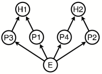
Figure 1: The food web used in simulated time-series. The food web consists of two herbivores each feeding predominantly on pairs of plants. However, for each pair of species a feeding link is possible in one direction, so more completely connected webs can exist for sub-optimal foraging. The species designations are given in ascending order of population in the parent model. The environment species, E, has either a fixed population or a fixed birth rate.

community grown in the equation-based model, was used to provide a community of species with established feeding links. Individuals of the resource species, E, are added at a constant rate, $\rho$, and are subject to ‘death’ at rate $d$ in the same way as all other species. It was experimentally determined that, for a $100\times 100$ lattice with periodic boundary conditions, an interval between agent movements of $\tau=9174^{-1}$ was needed to match the unit expectation time in the parent model of two individuals meeting. The closest match to the steady-state strategy of the parent model was built by allocating individuals of each species to pure foraging strategies according to the ESS, $f_{ij}$ as calculated from (5). The strategy of new-born individuals was copied from their parent with mutation, such that the probability of attacking each prey species was adjusted by 5%, then rescaled to make the greatest probability $1.0$. Fraction $\mu=0.01$ of new-borns were assigned an additional prey species chosen at random from the ESS, which they attack with probability $0.5$ if it was not already assigned a non-zero probability. From these initial conditions, Figure 2 shows that after

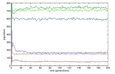
Figure 2: The ensemble-average time-series of 20 simulation runs, sampled at approximately unit intervals. In order of ascending population at time 200 the species are; H1, H2, P1, P2, P4, and P3.

approximately twenty generations, the population of each species has settled to an approximately steady value. The ratio of these populations are not quite the same as for the parent model, but it is sufficiently remarkable that the model is able to support food webs built in the parent model without substantial reconfiguration, given the gap between the competition models.

For comparison, the agent-based model was run from an initial condition in which all prey corresponding to positive $S_{ij}$ are attacked. In this case, for each pair of species $i,j\neq i$ either $S_{ij}$ or $S_{ji}$ is positive, and hence one species will definitely attack the other when encountered. Where $S_{ij}$ is very small this can be very far from the optimal strategy, to the extent that no feeding link exists in the parent model. The ensemble-average time series shown in Figure 3 covers a much longer

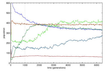
Figure 3: The ensemble-average time-series of 20 simulation runs, binned to intervals of 20 generations. In order of ascending population at time 1000 (marked) the species are; H1, P2, P4, P3, H2, and P1.

period of time than does Figure 2, yet even after this period the system has not reached a steady state. Examination of the single time series shown in Figure 4 illustrates the underlying cause of the gradually changing populations seen in Figure 3. In any given simulation run, there exist states in which the population of each species is not changing systematically with time to any great degree, but which are interrupted by rapid transitions to a different configuration of populations. The change takes place over a few generations, and is caused by the rapid propagation of a superior foraging strategy through one species.

The four periods marked in Fig. 4 clearly differ in the relative populations of the six species and, apart from stochastic effects, do not appear to contain systematic changes in those populations. To understand the cause of the differences, the effective food web was calculated for each period by counting the number of occasions on which each species consumed each possible prey. The essential difference between successive periods is the loss of a single feeding strategy by one species. By the time of the first marked period, only three strategies had been lost from the fully-connected food web of the initial condition; species P3 was no longer fed on by either species P2 or P4, accounting for its increase in abundance after an early low, and P4 had also ceased feeding on P2. By the second period, P1 had also stopped feeding on P3, and it stopped feeding on P4 by the third period. In each case the predator population was decreased by adopting a strategy for which individual fitness was improved. By the final period, H1 had stopped feeding on P2, but two very significant differences from the parent configuration remain. In the first place, ‘plant’ P1 still fed on P2 rather than becoming truly basal. Secondly, and with great significance to the relative populations, H2 still fed upon the environment directly.

Allowed sufficient time, the food web configuration present in the ensemble of Figure 2 might be recovered, but the timescale is extremely long. An increase in the resource availability by a factor of two appears to slow the transitions by approximately a factor of four, but reducing the resources by a similar factor results in almost all cases in the extinction of P3 during its early under-abundant phase. It has therefore not been possible to test for the complete convergence of the ensembles shown in Figures 2 and 3, and consequently it has not been demonstrated that the agent-based model will converge on the same configuration as the parent model.

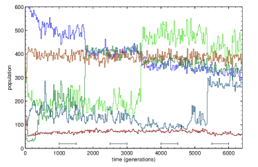
Figure 4: A sample time-series, binned to intervals of 20 generations. The feeding strategy of the agents was determined within each of the four marked intervals. Species P1 and H2 initially have the highest and second-highest populations respectively, while H1 has the lowest population after time 500. The three transitions to larger populations are made, in chronological order, by species P3, P4, and P2.

V Conclusions

An agent-based approach is a natural level of detail at which to examine a number of phenomena important to the formation of food web structures in related models. In particular, evolutionary mechanisms operate at this level, and predictions regarding the population-level behaviour of an evolving system need to be tested by comparison with the predictions of simulations of individuals, especially where other experimental confirmation is not possible. A surprising outcome of the simulations of the agent-based model presented in this paper is that the approach to the evolutionary stable strategy assumed by earlier, population-level models is inhibited by increased populations to such a degree that the ESS may never be relevant to a food web continually perturbed by invasions, extrinsic fluctuations, and spatial inhomogeneity. The computational demands of agent-based simulation, as compared to equation-based models of population dynamics, make the more detailed model inappropriate for examining evolutionary time-scales, but an investigation of the assembly of immigrant communities under agent-based dynamics is feasible. An essential aspect of future investigation is to relate the agent- and the equation-based models not merely in terms of mean behaviour, but in understanding and predicting the deviations of the former model from that mean.

Two related aspects of the approach to agent-based modelling used are of particular value. On the one hand, the process of developing an agent-based model provides insight into implicit assumptions about the mechanisms being used. Where population-level equations have been chosen to reproduce observed phenomena this can lead to understanding of the particular interactions which are necessary to reproduce the observations. On the other hand, much insight from behavioural biologists and ecologists can be incorporated into a model only at the level of interactions between individuals, since the consequences of including these effects are not know a priori. The development of a generic food web model into which these effects can be incorporated is therefore of great potential value, especially as the model is already known to be able to reproduce a number of ecological results relating to food web function and species populations.

Appendix A Model Description

This section provides a specification for the agent-based Webworld model based on the template of Grimm et al. (2006). Further details of the model at the population level can be found in Caldarelli et al. (1998) and Drossel et al. (2001).

A.1 Purpose

The purpose of the model is to reproduce the Webworld model of food web assembly in an agent-based formulation. The derivation of the model gives insight into the mechanisms implicitly underlying the earlier model, and the use of an agent-based framework lays the foundations for future abstract models to incorporate more realistic ecological detail.

A.2 State variables

The model comprises species, identical in description to those used in earlier, non-agent-based papers, individuals, and a spatial lattice. Individuals are characterised by the state variables: species, vulnerabilities, strategy, birth date, date of next action, a direction, and a three-valued discrete variable recording whether the individual is foraging, tired, or sated. Global variables are given in Table 1.

Symbol	Description	Value
$b$	Time scale for ‘digestion’	0.005
$d^{-1}$	Maximum life span	1.0
	of individual
$\lambda$	Ecological efficiency/	0.1
	probability of reproduction
$\mu$	Probability of acquiring	0.01
	new prey
$\rho$	Rate of introduction of	50 000
	resource individuals
$\tau$	Time interval for movement	$9174^{-1}$

Table 1: Global constants of the agent-based Webworld model. $\rho$ is chosen to determine the final population size and/or number of species.

The species is a set of $L=10$ attributes chosen from $K=500$ possibilities. For each pair of species $i,j$, these determine the score of $i$ when feeding on $j$, $S_{ij}=-S_{ji}$, calculated using (1). Negative values of $S_{ij}$ are never used. Species are evolved by mutation and selection as described by Drossel et al. (2001). A constraint on the set of attributes is that the $L$ attributes must all be different, and that species must differ in at least one attribute.

The vulnerabilities are a set of $V=33$ attributes chosen from the same set as the species attributes. These are chosen at birth from a uniform distribution, with the condition that the $V$ attributes are all different.

The strategy of an agent is an associative array of species and probabilities. The array must contain at least one species with associated probability 1, and does not contain any species, $j$, for which $S_{ij}\leq 0$, where $i$ is the species of the agent. For each species not represented in the array, the probability is assumed to be zero. Conceptually, the offspring of an agent adopt the same set of prey species with slightly altered probabilities, and therefore cannot normally feed on prey species which were unknown to their parent.

The birth date and date of next action are used to determine the life history of the individual as specified in the next section.

The lattice associates each individual with one lattice point, and represents a two-dimensional Cartesian space with periodic boundaries to model a well-mixed spatial distribution.

Individuals of the special ‘resource’ species are introduced at rate $\rho$. Individuals of this species can be attacked in the same manner as a normal species, but cannot themselves attack. They are assumed to always be in the ‘foraging’ state.

Species	Attributes
E	10, 33, 60, 78, 114, 260, 342, 346, 391, 428
P1	81, 204, 217, 240, 328, 335, 357, 368, 388, 467
P2	1, 43, 156, 165, 210, 220, 250, 320, 368, 481
P3	127, 130, 183, 193, 204, 210, 225, 240, 481, 467
P4	43, 80, 193, 217, 320, 390, 400, 425, 446, 470
H1	5, 31, 224, 332, 367, 374, 450, 459, 463, 495
H2	73, 211, 252, 294, 297, 330, 336, 370, 384, 466

Table 2: Attributes of the co-evolved species in the small community used for the simulation results of this paper.

A.3 Process overview and scheduling

The model proceeds by discrete events, and has an internal date variable to represent the most recent event. Each agent acts either on its internal date-of-next-action or time $d^{-1}$ after its birth, whichever the sooner. In the latter case the agent simply dies, and is removed from the model. The model identifies the agent with the earliest date, choosing at random between agents that happen to have the same date, typically due to the limits of numerical precision. Before the selected agent acts, new resources are added to the system according to a Poisson distribution with expectation value $\rho\delta t$, where $\delta t$ is the difference between the agent’s date of action and the date of the most recent event. Like ‘real’ individuals, resources are removed from the model time $d^{-1}$ after they are added. The action that the agent takes depends on its state. If the agent is tired, it enters the foraging state, and schedules a date $\tau$ later on which to move. An agent does the same if it is sated, except that in this case it reproduces with probability $\lambda$. The creation of the offspring is detailed below. If the agent is neither tired nor sated, it must be foraging, and the event is one of movement.

Movement occurs on the spatial lattice. The value of $\tau$ given in Table 1 corresponds to a square lattice of $100\times 100$ points, with periodic boundaries. To promote mixing, agents move in the same direction as their previous movement with probability $\frac{1}{2}$, or move to the left or right of that direction with probability $\frac{1}{4}$ in each case. Other movement schemes may be preferred but have not been investigated. On the arrival of agent X at the new lattice point, all foraging agents present are placed in a queue in random order. Agents which are not foraging cannot predate on agent X, and are assumed to be concealed such that they cannot be predated themselves. For each agent in the queue in turn, agent X and the queued agent are each given the opportunity to attack one another. Because $S_{ij}=-S_{ji}$ for any species $i$ and $j$, mutual predation and cannibalism is forbidden in Webworld, and hence for any pair of individuals at most one will attack. If X still exists and is still in the foraging state, the interaction with the next agent in the queue is investigated. If X remains in the foraging state after all possible interactions have been considered, it schedules a movement action after time $\tau$.

	Prey
Predator	E	P1	P2	P3	P4	H1
P1	5.599		1.924	0.7194	0.9849
P2	5.586			0.2975
P3	5.72
P4	5.885		0.1906	0.4078
H1		3.096	0.5075	4.829	0.4491
H2	0.1252	1.54	4.781	0.582	2.793	0.6788

Table 3: Scores of the small community used for the simulation results of this paper. Non-positive scores are omitted for simplicity.

When agent Y is given the chance to attack agent Z, it examines its strategy to determine the result, based on the species of Z. If Y attacks, it discovers whether or not Z has a vulnerability to Y’s species. If so, the attack is successful, in which case Z is destroyed and Y enters the sated state. If Z is not vulnerable to Y’s species, Y enters the tired state, but Z is unaltered. In particular, Z does not cease foraging. In either case, Y is no longer foraging, and reschedules its next action to occur after time $b/S_{ij}$, where $i$ is the species of Y and $j$ is the species of Z.

Offspring are added to the system as copies of their (single) parent in the same location. Their birth date is set, fixing the latest date at which they might die, and they schedule a movement action for time $\tau$ after their birth. The vulnerabilities of the offspring are generated as a random selection of the $K$ species attributes, without repetition. For each species in the parent’s strategy, the probability of attacking that species is modified $\pm 0.05$, then scaled such that the maximum probability is 1. If any ‘probability’ has become less than or equal to zero, the corresponding species is removed from the strategy. With probability $\mu$, the ESS of the species is calculated using (4) and (5), and one prey species selected using the ESS as a probability distribution. If the offspring’s strategy does not contain that prey, it is added with probability of attack equal to 0.5.

A.4 Design concepts

Emergence: Although there exists an expected behaviour of each species according to the parent model, the strategy in fact allows the emergence of a food web configuration given an arbitrary set of species. When evolution or immigration of new species occurs, the balance of introduction and extinction causes an emergent food web configuration.

Species	E	P1	P2	P3	P4	H1	H2
Population	20000	87	335	449	524	26	91

Table 4: Initial populations used in the agent-based simulations. These reflect the steady-state populations of the parent model, scaled by a factor of 20 to reduce stochastic extinctions.

Adaptation: On short time scales, the strategy of agents is subject to selection. The strategy of a population of agents should approximate the ESS of the parent model, which is found explicitly. On longer time scales, species are introduced as mutants of existing species in the same manner as in the parent model. These species co-evolve to promote adaptation between predators and prey.

Fitness: Fitness is implicitly modelled as the time taken for an individual to reproduce. Individuals successful in identifying prey species susceptible to attack, and which correspond to large score values, will reproduce rapidly and hence increase in abundance. Individuals are implicitly unfit if they are vulnerable to abundant predators, but vulnerability traits are not inherited and hence no selection operates.

Prediction: Agents do not possess any degree of reasoning, and do not even adjust their strategy according to their life history. Natural selection adjusts the mean strategy of each species to suit the expected success rate of feeding on each prey species.

Sensing: Individuals are able to sense only the species to which other individuals belong.

Interaction: All interactions between individuals are of a predatory nature.

Stochasticity: The movement of individuals on the lattice is stochastic, and the decision to attack prey is stochastic if more than one prey species is known. On evolutionary time-scales, the mutations available to species are stochastic, allowing selection to drive the evolution of the ecology.

Collectives: The only collective entities in the model per se are species, which dictate the possible interactions between individuals.

Observation: Intended observations are the population of each species, and the strategy averaged over all individuals of each species. The latter is a proxy for the strategy, $f_{ij}$, measured in the parent model.

A.5 Initialization

For the results in this paper, the model was initialized from a small community of species grown in the parent model. Using an arbitrary population multiplier, individuals were placed in the model in proportion to the species population in the parent model. Vulnerabilities were assigned at random, although this cannot be the steady-state configuration since individuals vulnerable to extant predators are depleted. For the results most like the parent model, strategies were initially assigned by dividing agents into groups according to the ESS. Subject to rounding, fraction $f_{ij}$ of the individuals of species $i$ were assigned a ‘pure’ strategy consisting of attacking species $j$ with probability 1. Agents, and resources in an abundance specified as an initial condition, were scattered at random on the lattice with random direction.

For the simulation runs presented in this paper, Table 2 details the species present, an overview of the food web being shown in Fig. 1. The scores which lead to the feeding relations and the behaviour of the agent-based model are given in Table 3. All simulation runs were initialized with the populations shown in Table 4.

A.6 Input

Resources are added to the system at a constant rate, allowing resource influx to balance resource consumption and ‘death’. Species can be added as mutants of existing species by changing one attribute, or from a community evolved previously, perhaps in the parent model.

References

- Grimm and Railsback (2005) Grimm, V., Railsback, S. F., 2005. Individual-based Modeling and Ecology. Princeton University Press, NJ.
- Bell et al. (2006) Bell, T., Freckleton, R. P., Lewis, O. T., 2006. Plant pathogens drive density-dependent seedling mortality in a tropical tree. Ecology Letters 9, 569–574.
- Condit et al. (1992) Condit, R., Hubbell, S. P., Foster, R. B., 1992. Recruitment near conspecific adults and the maintenance of tree and shrub diversity in a neotropical forest. American Naturalist 140, 261–286.
- Stephens et al. (2002) Stephens, D. W., McLinn, C. M., Stevens, J. R., 2002. Discounting and reciprocity in an Iterated Prisoner’s Dilemma. Science 298, 2216–2218.
- Brewer (2008) Brewer, S., 2008. Declines in plant species richness and endemic plant species in longleaf pine savannas invaded by Imperata cylindrica. Biol. Invasions 10, 1257–1264.
- Wilkinson (2004) Wilkinson, D. M., 2004. The parable of Green Mountain: Ascension Island, ecosystem construction and ecological fitting. J. Biogeogr. 31, 1–4.
- Blount et al. (2008) Blount, Z. D., Borland, C. Z., Lenski, R. E., 2008. Historical contingency and the evolution of a key innovation in an experimental population of Escherichia coli. PNAS 105, 7899–7906.
- Srivastava et al. (2004) Srivastava, D. S., Kolasa, J., Bengtsson, J., Gonzalez, A., Lawler, S. P., Miller, T. E., Munguia, P., Romanuk, T., Schneider, D. C., Trzcinski, M. K., 2004. Are natural microcosms useful model systems for ecology? Trends in Ecology and Evolution 19, 379–384.
- Wyszomirski et al. (1999) Wyszomirski, T., Wyszomirska, I., Jarzynaa, I., 1999. Simple mechanisms of size distribution dynamics in crowded and uncrowded virtual monocultures. Ecological Modelling 115, 253–273.
- Gotelli and Ellison (2006) Gotelli, N. J., Ellison, A. M., 2006. Food-web models predict species abundances in response to habitat change. PLoS Biology 10, 1869–1873.
- Hölker and Breckling (2005) Hölker, F., Breckling, B., 2005. A spatiotemporal individual-based fish model to investigate emergent properties at the organismal and the population level. Ecological Modelling 186, 406–426.
- Reuter (2005) Reuter, H., 2005. Community processes as emergent properties: Modelling multilevel interaction in small mammals communities. Ecological Modelling 186, 427–446.
- Vlachos et al. (2004) Vlachos, C., Gregory, R., Paton, R. C., Saunders, J. R., Wu, Q. H., 2004. Individual-based modelling of bacterial ecologies and evolution. Comparative and Functional Genomics 5, 100–104.
- Caldarelli et al. (1998) Caldarelli, G., Higgs, P. G., McKane, A. J., 1998. Modelling coevolution in multispecies communities. J. Theor. Biol. 193, 345–358.
- Drossel et al. (2001) Drossel, B., Higgs, P. G., McKane, A. J., 2001. The influence of predator-prey population dynamics on the long term evolution of food web structure. J. Theor. Biol. 208, 91–107.
- Drossel et al. (2004) Drossel, B., McKane, A. J., Quince, C., 2004. The impact of nonlinear functional responses on the long-term evolution of food web structure. J. Theor. Biol. 229, 539–548.
- Quince et al. (2005) Quince, C., Higgs, P. G., McKane, A. J., 2005. Topological structure and interaction strengths in model food webs. Ecol. Model. 187, 389–412.
- Lugo and McKane (2008) Lugo, C. A., McKane, A. J., 2008. The characteristics of species in an evolutionary food web model. J. Theor. Biol. 252, 649–661.
- Powell and McKane (submitted) Powell, C. R., McKane, A. J., submitted. Comparison of food webs constructed by evolution and by immigration, arXiv:0808.2922v1.
- Powell and Boland (accepted) Powell, C. R., Boland, R. P., accepted. The effects of stochastic population dynamics on food web structure, arXiv:0805.0084v1.
- Rademacher et al. (2004) Rademacher, C., Neuert, C., Grundmann, V., Wissel, C., Grimm, V., 2004. Reconstructing spatiotemporal dynamics of Central European natural beech forests: the rule-based forest model BEFORE. Forest Ecology and Management 194, 349–368.
- Petermann et al. (2008) Petermann, J. S., Fergus, A. J. F., Turnbull, L. A., Schmid, B., 2008. Janzen-Connell effects are widespread and strong enough to maintain diversity in grasslands. Ecology 89, 2399–2406.
- Pickering (1917) Pickering, S., 1917. The effect of one plant on another. Annals of Botany 31, 181–187.
- Grimm et al. (2006) Grimm, V., Berger, U., Bastiansen, F., Eliassen, S., Ginot, V., Giske, J., Goss-Custard, J., Grand, T., Heinz, S. K., Huse, G., Huth, A., Jepsen, J. U., Jorgensen, C., Mooij, W. M., Muller, B., Pe’er, G., Piou, C., Railsback, S. F., Robbins, A. M., Robbins, M. M., Rossmanith, E., Rueger, N., Strand, E., Souissi, S., Stillman, R. A., Vabo, R., Visser, U., DeAngelis, D. L., 2006. A standard protocol for describing individual-based and agent-based models. Ecological Modelling 198, 115–126.
- Lima and Dill (1990) Lima, S. L., Dill, L. M., 1990. Behavioral decisions made under the risk of predation: a review and prospectus. Canadian Journal of Zoology 68, 619–640.