Theory Summary: International Symposium on Multiparticle Dynamics 2008

Abstract

I summarize the theory talks presented at the International Symposium on Multiparticle Dynamics 2008.

1 Introduction

The XXXVIII International Symposium on Multiparticle Dynamics (ISMD 2008) covered a wide variety of topics in nuclear and particle physics. The organizers had an interesting idea of arranging all the topics on a single plot in the $(\ln Q^{2},\ln 1/x_{Bj})$-plane, as shown in the conference poster. I think the idea of such classification on such a broad scale is new and interesting: in Fig. 1 I present my own version of the classification proposed by the organizers with some slight modifications as compared to the original. Fig. 1 gives the summary of the topics covered during the conference: below I will discuss each of the topics shown in Fig. 1 in a separate Section.

Indeed no classification can adequately reflect all the subtleties of each of the topics discussed. The classification of Fig. 1 is no exception. Many of the subjects shown have a lot more dimensions to them (in some cases literally so) than shown in Fig. 1.

The idea of mapping out the $(\ln Q^{2},\ln 1/x_{Bj})$-plane comes from the physics of parton saturation at small Bjorken $x$, also known as the Color Glass Condensate (CGC) (for a review see [1]). It appears that this approach could be generalized beyond small-$x$ physics. One of the main concepts of CGC is that at small enough $x$ the gluon density in the proton or nuclear wave functions gets so high that non-linear effects, such as parton mergers, become important leading to saturation of gluon and quark distribution functions. The transition to this saturation regime is described by the saturation scale $Q_{s}$, which is a function of $x$. $Q_{s}$ increases as $x$ decreases. Saturation region is schematically represented by a yellow triangle in Fig. 1. Indeed strong interaction physics below the confinement scale, at $Q^{2}<\Lambda^{2}_{\mathrm{QCD}}$, is non-perturbative. The non-perturbative large-coupling region is denoted in Fig. 1 by a blue rectangle. At small enough $x$ the saturation scale becomes larger than $\Lambda_{\mathrm{QCD}}$: therefore the saturation regime lies in the perturbative region to the right of $\Lambda_{\mathrm{QCD}}$.

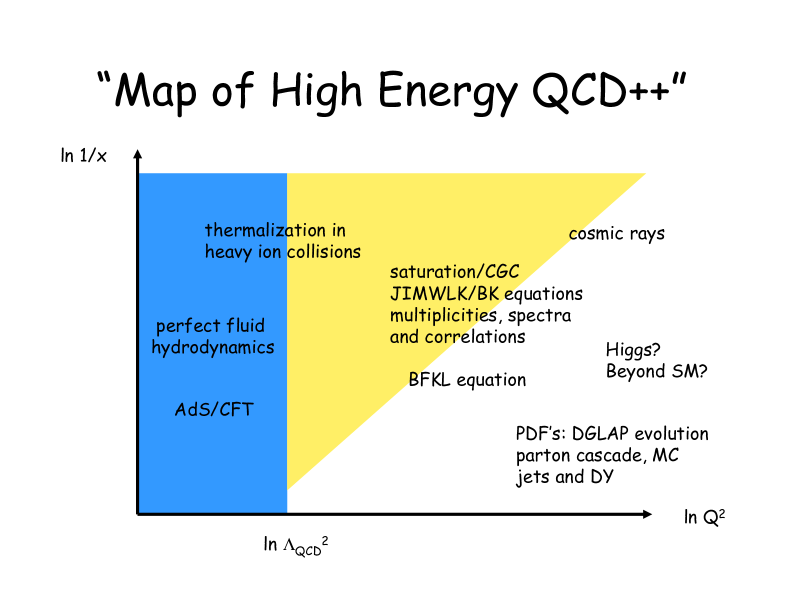
Figure 1: My own version of arranging all the topics covered during the conference in the $(\ln Q^{2},\ln 1/x_{Bj})$-plane. The idea was borrowed from the conference poster with the topics somewhat modified and moved around.

The large-$Q^{2}$ region with not very small $x$ is the domain of linear DGLAP evolution equation [2, 3, 4]. This is the region where collinear factorization applies. The approaches based on collinear factorization, such as parton cascade simulations and jet physics in general, also belong in that region. Some of the topics discussed in that subfield will be described in Sect. 2 below. As one moves towards smaller $x$ (and somewhat lower $Q^{2}$) the logarithms of $1/x$ become important. Such logarithms are resummed by the BFKL equation [5, 6]. Progress in our understanding of BFKL will be reviewed in Sect. 3. Moving on toward even lower $x$ one crosses the saturation line and enters the saturation/CGC region. Here the nonlinear JIMWLK [7, 8] and BK [9, 10] evolution equations apply. I have also grouped in this region of the map the predictions of CGC physics for various $AA$, $pA$ and $pp$ observables. The talks on this topic will be discussed in Sect. 4. All the small-$x$ machinery should be directly applicable to cosmic ray physics: the progress in this direction will be mentioned in Sect. 5. Heavy ion physics poses a number of important questions for theorists. Over the past several years a consensus has been reached in the heavy ion community that heavy ion collisions at RHIC lead to the creation of a strongly-coupled quark-gluon plasma (QGP). The challenges facing the heavy ion theory community include understanding of the creation of such medium: how do the particles produced in a collision thermalize to form the strongly-coupled QGP? The mechanism leading to the creation of strongly-coupled QGP may or may not be perturbative, as reflected in Fig. 1. The talks on this subjects will be reviewed in Sect. 6. The subsequent evolution of the produced medium governed by the perfect fluid or viscous hydrodynamics will be discussed in Sect. 7. Developments in Anti-de Sitter/Conformal Field Theory (AdS/CFT) correspondence, which can shed light on many topics in heavy ion collisions, deep inelastic scattering (DIS), and hadronic scattering, will be reviewed in Sect. 8. Finally, the Higgs boson and physics beyond Standard Model are placed at large $Q^{2}$ and at large energy/small-$x$ in Fig. 1: they will be mentioned in Sect. 9.

ISMD 2008 featured a large number of very interesting talks. I have to apologize beforehand for not being able to cover all of them due to space limitations. Also, when describing work presented at ISMD 2008 I will not provide explicit citations to the corresponding publications, assuming that interested readers could find the needed references in the Proceedings contributions of the corresponding speakers. Finally, as this is not a review article, in presenting the topics I will not spend much time recounting many important successes in each subfield, but will concentrate instead on open problems at the forefront of research.

2 PDF’s, parton cascades and jets

Much of our knowledge about QCD at high energies comes from and could be summarized in parton distribution functions (PDF’s). Our current knowledge of PDF’s was summarized in the talk by Stirling. Fig. 2 presents the proton PDF’s at $Q^{2}=10$ GeV² given by the MSTW 2007 parameterization.

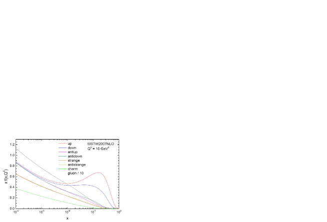
Figure 2: PDF’s in the MSTW 2007 parameterization (from the talk by Stirling).

There has been much improvement in our understanding of PDF’s in recent years. Error analysis have been carried out and now many PDF’s come with error bars, as demonstrated in Fig. 3 shown in the talk by Rojo-Chacon. Fig. 3 shows singlet and gluon distribution functions at $Q_{0}^{2}=2$ GeV² due to CTEQ, MRST/MSTW, Alekhin and NNPDF collaborations [11, 12, 13, 14] along with the error bars. We see that in the small-$x$ region PDF uncertainties are large. They appear to increase as we go toward lower Bjorken $x$ into the region where there is no data.

The lower panel of Fig. 3 also shows that at small-$x$ and small-$Q^{2}$ the gluon distribution function becomes negative. This issue had been discussed a lot over the past years, and received a lot of attention at ISMD 2008 as well. The question is whether a negative gluon distribution necessarily implies a breakdown of the approach based on the linear DGLAP evolution equation. The standard argument against DGLAP breakdown is that at small $Q^{2}$ the expectation value of the operator identified with the gluon distribution function does not anymore count the number of gluons. Therefore no fundamental law is violated if it goes negative. As was brought up in the discussion session by Cooper-Sakar, one has to look at the structure function $F_{L}$, which is closely related to the gluon distribution function. $F_{L}$ is indeed a physical observable expressible in terms of scattering cross sections: it has to be positive. If $F_{L}$ resulting from the gluon distribution functions in the lower panel of Fig. 3 remains positive, then one could argue that there is no problem with the negative gluon distribution function. As indeed the $F_{L}$’s obtained from the gluon distribution functions in Fig. 3 appear to be positive one indeed can argue that negative $xG$ are allowed.

To me such arguments sound a bit like epicycles in Ptolemaic astronomy: some of our colleagues are trying to rescue a theory in trouble. Strictly-speaking it is true that there is nothing requiring $xG$ to be positive definite everywhere. However, I spent many years calculating $xG$ at small-$x$ in the perturbative (saturation) framework and never saw it go negative. It would be interesting and convincing if the proponents of negative $xG$ could come up with a (purely theoretical) model for gluon distribution, where everything is perturbative and under calculational control, and where $xG$ does become negative at small-$x$ and small-$Q^{2}$. For instance one could study gluon distribution in a very heavy quarkonium. Large quark masses would insure small coupling allowing to calculate $xG$ perturbatively from first principles. If negativity of $xG$ at low-$x$ and low-$Q^{2}$ is a natural property of the gluon distribution operator, it should come out straightforwardly in such a calculation.

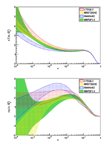
Figure 3: Singlet and gluon distribution function at $Q_{0}^{2}=2$ GeV² due to different PDF collaborations with the error bars shown (from the talk by Rojo-Chacon).

Parton cascades as the way to model actual collisions on the event-by-event basis received a lot of attention at ISMD 2008 as well with a nice review talk by Z. Nagy. The ideas of going beyond collinear factorization and including $k_{T}$-dependent effects into parton cascades were discussed by Hautmann. Problems with Monte Carlo simulations of small-$x$ coherent effects were discussed in the talk by Marchesini. There is a difficult problem that arises when one tries to include recoil effects into the color-dipole parton cascades in a probabilistic QCD picture.

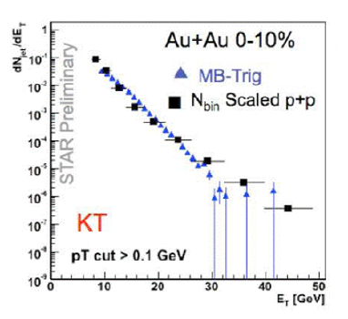
Figure 4: Preliminary STAR collaboration data on the number of jets as a function of $E_{T}$ of the jet for central $Au+Au$ collisions (triangles) and for proton-proton collisions scaled up by the number of binary collisions (squares). (Picture is from the talk by Rojo-Chacon, originally taken from [15].)

There were several good talks on jet analysis and algorithms. I was particularly interested to see jet analyses coming to RHIC. The suppression of high-$p_{T}$ hadrons produced in $Au+Au$ collisions at RHIC as compared to $p+p$ collisions scaled up by the number of binary collisions is believed to be one of the smoking guns for the creation of a hot and dense medium in heavy ion collisions, likely to be a thermalized quark-gluon plasma (QGP) [16, 17, 18]. The suppression is quantified with the help of the nuclear modification factor $R^{AA}$. The suppression was observed in RHIC experiments at $\sqrt{s}=200$ GeV and attributed to parton energy loss also known as jet quenching. However one should not forget that in the $R^{AA}$ measurements one measures individual high-$p_{T}$ hadrons, and not proper jets. A jet analysis with a jet cone definition has recently been carried out by the STAR experiment. The preliminary results are shown in Fig. 4, which was shown at ISMD 2008 by Rojo-Chacon with a similar figure shown by Caines. Fig. 4 depicts the number of jets as a function of $E_{T}$ of the jet. In Fig. 4 the triangles denote the data for $Au+Au$ collisions, while the squares denote the $p+p$ data scaled up by the number of binary collisions. It is curious and a bit puzzling that no visible suppression of jets in $Au+Au$ compared to scaled-up $p+p$ was found (within error bars). One could speculate that the energy deposited by the hard parton into the medium is not simply absorbed by the medium, but instead travels along with the parton in the form of softer partons, such that the net energy in the jet cone does not change and the jet as a whole does not get suppressed. Indeed more work is needed to understand the data in Fig. 4.

3 The BFKL equation

The status of the linear BFKL evolution equation has been reviewed in the talk by White. The main problem with the linear BFKL evolution is the large and negative NLO BFKL correction to the pomeron intercept, which one obtains by using the NLO BFKL results of [19, 20] evaluated at the LO saddle point. The correction is so large that it makes the gluon distribution function fall off with decreasing $x$.

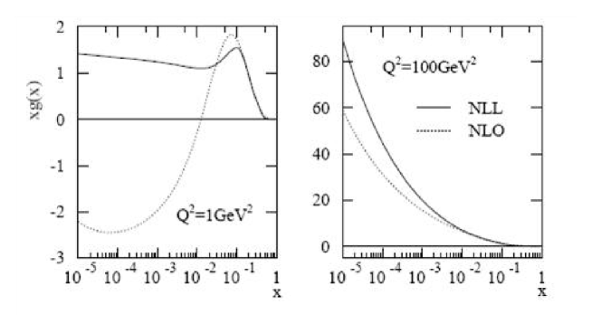
Figure 5: Gluon distribution function due to NLO BFKL corrections resummed in the TW prescription (solid lines) compared to the NLO DGLAP results (dotted lines). (Pictures are from the talk by White.)

Several ways to remedy this problem have been proposed. It was observed that going beyond the saddle point approximation, e.g. by solving the NLO BFKL equation numerically, significantly reduces the NLO correction to the intercept, making the resulting BFKL Green function rise with decreasing $x$ [21]. An alternative/complimentary way out involves resumming DGLAP transverse logarithms in the NLO BFKL kernel: one such procedure, pioneered by Ciafaloni, Colferai, Salam, and Stasto (CCSS) [22] also gives a positive pomeron intercept albeit somewhat smaller than the LO BFKL intercept. Other procedures involved are due to Altarelli, Ball, and Forte (ABF) [23] and Thorne and White (TW). The results of the TW resummation for the gluon distribution function are shown in Fig. 5 (solid lines) compared to the NLO DGLAP results (dotted lines). One can see that TW resummation cures the problem of the negative gluon distribution at low-$Q^{2}$ and low-$x$ that NLO DGLAP has. Still the gluon distribution in the left panel of Fig. 5 corresponding to $Q^{2}=1$ GeV² is almost flat as one goes toward lower $x$: it is unclear what physical mechanism would make $xG$ behave in such a way in the absence of saturation effects in the approach used.

Other problems of the linear BFKL evolution include violation of unitarity bound (or, more precisely, the black disk limit) and diffusion into the infrared. Those problems are remedied by the physics of parton saturation, to be discussed next.

4 Saturation/Color Glass Condensate

The talks by Golec-Biernat and by Marquet gave a nice introduction to the physics of parton saturation/CGC and the non-linear evolution equations involved [7, 8, 9, 10]. While the theoretical framework behind CGC is solid, the question of unique experimental detection of CGC is still debated. CGC prediction of hadron suppression at forward rapidities in the $d+Au$ collisions at RHIC [24, 25, 26] shown here in Fig. 6 were spectacularly confirmed by the data [27, 28, 29, 30]. The CGC prediction involved the conventional shadowing effects, which redistribute the partons through multiple rescatterings from lower $p_{T}$ to higher $p_{T}$, leading to low-$p_{T}$ suppression (shadowing) and high-$p_{T}$ enhancement (anti-shadowing) shown in the upper curve in Fig. 6. (The high-$p_{T}$ enhancement of produced particles is known as Cronin effect.) The effects of small-$x$ BFKL/JIMWLK/BK evolution equations (the saturation effects) lead to decrease of the number of produced particles (as compared to the $p+p$ reference) at all $p_{T}$, as shown by the dash-dotted, dashed, and the lower solid curves in Fig. 6 (for a review see [1]).

Figure 6: A sketch of the nuclear modification factor $R^{pA}$ as a function of the transverse momentum of the produced particle $k_{T}$ in the units of the saturation scale from [25]. The upper curve corresponds to the lowest energy/rapidity, while the other curves show what happens as the energy/rapidity increases.

However, as conventional approaches based on collinear factorization with significantly ad hoc modified nuclear shadowing have been able to describe the data a posteriori [31], the need arose for new experimental tests to uniquely disentangle between the collinear factorization scenario with shadowing included and the physics of CGC. One of such CGC predictions for a two-particle correlation function was shown by Marquet and is presented here in Fig. 7, which shows a two-hadron correlation function plotted versus the opening azimuthal angle between the two hadrons $\Delta\phi$. The trigger particle has rapidity $y_{1}=3.5$ and $p_{T1}=5$ GeV.

Figure 7: CGC prediction for the azimuthal dependence of the two-hadron correlation function for different values of the $p_{T}$ of the associate particle (from the talk by Marquet).

The associate particle has rapidity $y_{2}=2$. The transverse momentum of the associate particle $p_{T2}$ is different for different curves, as explained in Fig. 7. The CGC prediction is that as $p_{T2}$ gets lower and comes closer to the saturation scale $Q_{s}$ (which is of the order of $1-2$ GeV at RHIC), the saturation effects would “wash out” the back-to-back azimuthal correlations, leading to a decrease in the correlation function as predicted in Fig. 7. The experiments currently running at RHIC will be able to test this prediction.

Another test of CGC will come from the upcoming LHC heavy ion experiments. In heavy ion collisions it is hard to construct a rigorous CGC prediction, as the problem of particle production in CGC for the collision of two nuclei have not been solved analytically. One therefore constructs models based on $k_{T}$-factorization formula (proven for $p+A$ collisions in CGC in [32] but not proven for $A+A$) trying to mimic as close as possible the true CGC physics (see e.g. [33]). One of the less model-dependent predictions of such an approach is for the total charged hadron multiplicity in heavy ion collisions. Predictions for total charged hadron multiplicity in $Pb+Pb$ collisions at the LHC from the work of Albacete [34] were shown by Marquet and are reproduced here in Fig. 8.

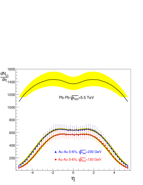
Figure 8: CGC prediction from [34] for the total charged hadron multiplicity in $Pb+Pb$ collisions at LHC, along with successful fits of the same quantity measured by RHIC at two different center-of-mass energies. The yellow band around the LHC prediction indicates the error bars.

The plot in Fig. 8 resulted from using the $k_{T}$-factorization formula also used in [33]. However, the dipole scattering amplitudes which enter that formula were evolved using the BK evolution equation with running coupling corrections, which have been recently calculated in [35, 36, 37]. Thus at least one of the ingredients used in arriving at Fig. 8 comes form a fairly rigorous CGC analysis, which has became available very recently and never has been used before. Based on that I believe that the prediction in Fig. 8 is the best theoretically-founded one. Unfortunately, due to limitations of our understanding of CGC mentioned above (concerning the applicability of the $k_{T}$-factorization formula to nucleus-nucleus collisions), the prediction in Fig. 8 still involves some degree of modeling that we can not control, and should thus be still taken with care.

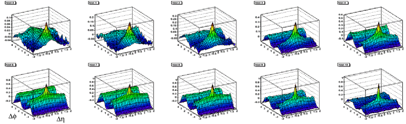
Figure 9: Two-hadron correlation function measured in $Au+Au$ collisions at RHIC as a function of rapidity interval between the two hadrons $\Delta\eta$ and the azimuthal angle between them $\Delta\phi$. Each panel corresponds to a different centrality of the collision. The data are from the STAR collaboration [38].

RHIC experiments continue to surprise us with an amazing quantity of interesting results. We now know the two-hadron correlation function as a function of both azimuthal angle between the hadrons and the rapidity interval between them, as shown in Fig. 9. The correlation function in Fig. 9 has at least one interesting unexplained feature: it has long-range rapidity correlations on the same azimuthal side ($\Delta\phi\approx 0$), known as “the ridge”. While many explanations were proposed, the feature remains largely unexplained. At ISMD 2008 McLerran proposed that “the ridge” could be due to long-range rapidity correlations inherent to CGC. Indeed CGC predicts rapidity correlations over the intervals of the order of $\Delta y\sim 1/\alpha_{s}$, which could be large if the strong coupling constant $\alpha_{s}$ is small. The radial flow would then boost the correlations, confining them to small azimuthal opening angles, thus creating a ridge-like structure. This is indeed a plausible explanation, but I feel more detailed theoretical work is needed to determine whether this is a unique prediction of CGC.

Another important feature of the two-hadron correlation function in $Au+Au$ collisions at RHIC is the double-hump structure shown in Fig. 10. Fig. 10 depicts the two-particle correlation function measured by PHENIX collaboration plotted as a function of the azimuthal angle between the two hadrons. As one can see from Fig. 10 the distribution of the associate particles as a function of azimuthal angle at low transverse momentum of the associate particle has two maxima. Assuming that the trigger particle travels through a relatively thin medium layer, one concludes that the associate particle is likely to travel through a thicker layer of the medium. The double-hump structure could therefore be caused by a Mach cone produced by a particle moving through a strongly-coupled medium [39]. Alternative explanation could be due to non-Abelian (QCD) Cherenkov radiation, as discussed in the talk by Dremin. To describe such radiation one has to solve classical Yang-Mills equations in a medium with some dielectric tensor. (While indeed Cherenkov radiation is a medium effect, the methods applied to the analysis are those of CGC, and hence I placed it in the CGC section.) Cherenkov radiation allows one to describe both STAR and PHENIX azimuthal correlations data by an appropriate choice of the dielectric tensor in the medium.

A possible signal of the creation of QGP in heavy ion collisions is the mass shift for the produced mesons due to medium effects. Padula suggested that a cleaner way to measure the shift would be by studying two-particle correlations of $\phi\phi$ and $K^{+}K^{-}$ pairs. Presence of the mass shift will be signaled by the appearance of back-to-back correlations in the $\phi\phi$ and $K^{+}K^{-}$ correlators.

Another interesting CGC prediction is for the rapidity distribution of the net baryon number produced in heavy ion collision. In the talk by Wolschin it was shown how CGC ideas allow one to successfully describe baryon number rapidity distribution at SPS and RHIC, and to even make predictions for LHC. It would be really interesting and important to measure this quantity at LHC.

A sign of the fact that CGC physics is entering a new era is the construction of event generators based on CGC concepts and ideas. In the talks by Avsar and Kutak we have heard about event generators using CCFM evolution equation with an infrared cutoff mimicking saturation/CGC effects, similar to how one can mimic the BK equation by using the BFKL equation with an infrared cutoff. Interesting results and fits were shown in those talks.

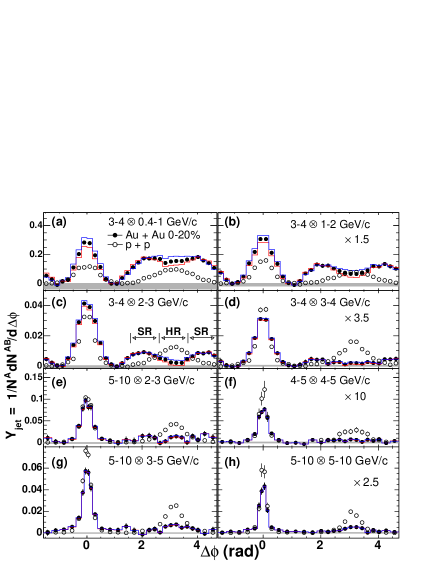
Figure 10: Two-hadron azimuthal correlation function as measured by PHENIX experiment (taken from [40]).

5 Cosmic rays

Ultra-high energy cosmic ray data and the accompanying theory was presented in the talks by Ostapchenko and Pierog. It was suggested that the existing discrepancy between the cosmic ray data and the conventional models may be explained by saturation/CGC effects. This is indeed an exciting prospect which needs to be pursued by CGC practitioners. The progress in this direction can however be marred by the fact that when extrapolating from current collider energies to the cosmic ray energies a large uncertainty arises due to the non-perturbative diffusion of the black disk. As was argued in [41] in perturbative CGC approach the diffusion of black disk at high energies is very fast: the radius of the disk grows as a power of energy due to the lack of a mass gap in perturbative approaches. Any attempt to non-perturbatively model the diffusion by introducing a mass gap into the problem leads to the radius of the black disk growing as a logarithm of energy. As the non-perturbative models are not under the same degree of theoretical control as the perturbative CGC calculations, the potential theoretical uncertainty associated with extrapolation to cosmic ray energies could be very large, leading to uncertainty both in total scattering cross sections and particle production cross sections calculated in CGC.

6 Thermalization in heavy ion collisions

Understanding the mechanism of thermalization and isotropization of the medium produced in heavy ion collisions is a very important open problem in the field.

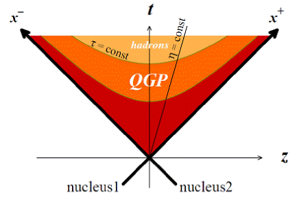
Figure 11: Space-time structure of a heavy ion collision (from the talk by Itakura).

The space-time structure of a heavy ion collision is depicted in Fig. 11. The time immediately after the collision is dominated by particle production. In that region CGC applies, such that the production of particles is described by perturbative CGC techniques. This stage of the evolution of the medium is sometimes referred to as “Glasma” [42], the term which combines the Color Glass physics (“Glas”) with the creation of quark-gluon plasma at later stages of the collision (“lasma”), as shown in Fig. 11. However the CGC dynamics by itself leads to a very anisotropic distribution of the produced matter in momentum space: the end result of CGC dynamics is a free-streaming “medium” with zero longitudinal pressure component. Indeed a thermalized medium should have all pressure components (transverse and longitudinal) equal, as it should be isotropic. Hence Color Glass itself does not lead to thermalization, or, more importantly, isotropization of the produced medium. (Isotropization is a necessary, but not a sufficient condition of thermalization.)

So how does Color Glass turn into a Glasma? One of the more popular scenarios was presented in the talk by Itakura and involves magnetic instabilities in the produced medium (see also [43, 44]). The main physical idea is that the momentum space anisotropy of the medium produced in heavy ion collisions would generate instabilities, which would rapidly isotropize the system leading to a hydrodynamic behavior of the medium. This indeed is a plausible scenario of thermalization/isotropization.

Since the saturation/Color Glass approach gives us a consistent framework in which all diagrams can be classified and resummed order-by-order, it is not at all clear why one has to separate the perturbative dynamics into a part which is incorporated in CGC and into everything else. From this standpoint the dynamics of instabilities would correspond to some higher order (quantum) corrections to the diagrams which we already know how to resum in the CGC approach. Such corrections would also be a part of CGC, just at some higher order. The magnetic instabilities could then be viewed as some higher order corrections to CGC which somehow got “out of control” and became very large (infinite?). Frankly I am skeptical whether such corrections exist: all our experience calculating CGC diagrams, both in the classical framework [45, 46, 47] and including (LO and NLO) quantum evolution and running coupling corrections [32, 48], never led to any uncontrolled infinities which would dominate the resulting production cross sections and the energy-momentum tensor. Perhaps the proponents of the instability-driven scenario should identify and resum diagrams with instabilities (starting from the very collision of two nuclei), and show that their contributions are really important (numerically or parametrically) and that these diagrams do lead to isotropization of the medium at late times. Implications of such diagrams on what we know in the standard perturbation theory in, say, proton-proton collisions would also have to be understood. One should also identify what those new instability diagrams have that was absent in the multitude of quantum corrections to the classical picture calculated over the years [32, 48].

Alternatively, as the medium created at RHIC is believed to be strongly-coupled, it is possible that thermalization and isotropization in heavy ion collisions are essentially non-perturbative (large-coupling) effects. Such a scenario can not be quantified in a controlled manner in QCD. However, AdS/CFT correspondence [49, 50] allows us to try to analyze this problem for the ${\cal N}=4$ Super Yang-Mills (SYM) theory. In my talk in the Dense Systems session I have presented one of the efforts in this direction. One could model a heavy ion collision as a collision of two shock waves in AdS₅. Solving Einstein equations in AdS₅ one can find the energy-momentum tensor of the resulting medium. It has been argued in [51] using AdS/CFT correspondence that if one assumes that the produced medium distribution is rapidity-independent, the strong-coupling dynamics would inevitably lead at late proper times to an isotropic medium described by Bjorken hydrodynamics [52]. However, it is not yet clear whether such a rapidity-independent distribution would result from a collision of two shock waves. Our result was that in a strongly-coupled theory the colliding shock waves would stop shortly after the collision. This seems like a natural result of the strong coupling effects. If the coupling is strong enough to stop the colliding nuclei, it is likely to quickly thermalize the system. However, a thermal system resulting from stopping of the nuclei is more likely to be described by rapidity-dependent Landau hydrodynamics [53], instead of the rapidity-independent Bjorken one. Hence the strong-coupling effects, if dominant throughout the collision, would not lead to Bjorken hydrodynamics. On top of that we know from the RHIC data on net baryon rapidity distribution that valence quarks in the nuclei do not stop in the collision, and instead (mostly) continue moving along the beam line [54]. Indeed the early stages of the collisions have to be described by the weak coupling effects, and are thus outside of the realm of the AdS/CFT correspondence. We presented a way of mimicking these weak-coupling effects in the dual AdS geometry. However, the question of what leads to Bjorken hydrodynamics still remains open.

7 Hydrodynamics

Regardless of our lack of understanding of thermalization in heavy ion collisions, the success of perfect-fluid hydrodynamics description of particle spectra and elliptic flow $v_{2}$ measured in the $Au+Au$ collisions at RHIC [55, 56] allows us to conclude that the medium created in the collisions is probably strongly coupled and that a hydrodynamic description of such medium is adequate.

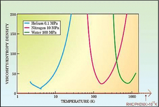
Figure 12: The shear viscosity-to-entropy density ratio (in units of $1/4\pi$) for various media (from the talk by Csörgő).

The Kovtun, Son, Starinets, Policastro (KPSS) [57, 58] lower bound on the ratio of shear viscosity $\eta$ to the entropy density $S$ derived from AdS/CFT correspondence was discussed in the talk by Csörgő. The KPSS bound postulates that for any medium (or, more precisely, for any theory with a gravity dual) one has $\eta/S\geq 1/4\pi$. Fig. 12 shows the ratio of $\eta/S$ plotted as a function of temperature for several different media with the KPSS bound shown by a straight horizontal line at the bottom. Csörgő pointed out that as RHIC data is consistent with a very low value of $\eta/S$, it is likely that RHIC fluid is more perfect than any other known fluid. This superfluidity also takes place at an extremely high temperature, characteristic of the QGP. However it is still possible that RHIC data allows for higher values of $\eta/S$ than $1/4\pi$: by varying the initial conditions for hydrodynamics one can accommodate somewhat larger values of $\eta/S$, though the exact values are still under investigation. There have also been some recent results in string theory suggesting that the KPSS bound might be violated in some theories due to stringy (mostly $1/N_{c}$) corrections. Regardless of that, the low viscosity of the RHIC QGP still strongly suggests that the medium created in the collisions is strongly-coupled.

Hydrodynamics is an exciting subfield by itself, allowing for many interesting exact solutions describing possible evolutions of RHIC fireball. Many of those solutions have been reviewed in the talk by M. Nagy, and fall into two main categories: relativistic and non-relativistic ones.

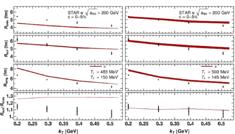
Figure 13: HBT radii at RHIC compared to hydrodynamic simulations with the standard (Glauber) initial conditions (left panels) and the Glauber initial conditions proposed by Florkowski (right panels). (The picture is taken from the talk by Florkowski.)

There are still open problems with the hydrodynamic description of the medium produced in RHIC collisions. One is the early thermalization proper time of $\tau_{0}=0.3\div 0.5$ fm/c required for hydrodynamics to describe the data: this problem is related to our (lack of) understanding of thermalization/isotropization in heavy ion collisions. Another problem concerns the HBT radii. While hydrodynamics is successful in describing particle spectra and $v_{2}$ [55, 56], it has been having problems describing HBT radii. This has been known as the RHIC HBT puzzle (see e.g. [59]). At ISMD 2008 Florkowski suggested that one could modify the standard Glauber initial conditions for hydrodynamics simulations: he suggested starting the simulations with a smaller Gaussian source, which would generate faster initial expansion. Apparently this approach worked, allowing to describe the HBT radii, as shown in Fig. 13, using a rather small set of free parameters. The obtained value for one of the parameters, the thermalization time $\tau_{0}$, turns out to be $\tau_{0}=0.25$ fm/c, which is rather close to some recent estimates based on AdS/CFT approaches [60].

While the approach presented by Florkowski works very well, as can be clearly seen from Fig. 13, one may worry that the initial size of the Gaussian fireball used is rather small to adequately describe realistic $Au+Au$ collisions. Therefore in my opinion the conclusion one can draw from the Gaussian initial conditions analysis is that in the simulations of Fig. 13 it mimics some initial time dynamics which leads to hydrodynamics being initialized with a pretty strong radial flow. It appears then that in order to describe the HBT radii one needs the initial conditions for hydrodynamics simulations to contain large flow in them. The exact nature of such initial dynamics still needs to be identified: it might be given by the CGC physics.

The perfect fluid hydrodynamics appears to do a good job at RHIC. It is possible though that in heavy ion collisions at LHC the plasma that will be created will start out at higher temperature. This would lead to smaller coupling constant, thus possibly making the resulting plasma less strongly coupled. The viscous corrections in such case would get larger: one therefore needs to construct viscous hydrodynamics simulations to describe the dynamics of the medium to be produced in heavy ion collisions at the LHC. But what if viscous corrections are not enough? What if higher fluid velocity gradients would also become important? The dynamics of strongly coupled medium described by AdS/CFT correspondence contains the exact result, including all gradients of fluid velocity. While obtaining this exact solution from AdS/CFT correspondence appears to be rather complicated, one could calculate the viscosity and higher order coefficients in fluid velocity gradient expansion using AdS/CFT approach. The results of the project to calculate the coefficients needed to construct causal viscous hydrodynamics using the AdS/CFT correspondence were presented in the talk by Baier. The obtained coefficients could be used to construct strong-coupling predictions for LHC.

8 AdS/CFT correspondence

AdS/CFT correspondence [49, 50] is a very powerful new tool for studying non-perturbative aspects of gauge theories coming from string theory (for a review see [61]). AdS/CFT correspondence [49, 50] postulates a duality between the ${\cal N}=4$ SYM theory in 4 space-time dimensions and the type-IIB string theory in AdS${}_{5}\times$S⁵. The more widely used and better tested gauge-gravity duality suggests that ${\cal N}=4$ SYM theory in the large-$N_{c}$ large-$\lambda=g^{2}\,N_{c}$ limit is dual to classical super-gravity on AdS₅ ($\lambda$ is ’t Hooft’s coupling constant, $g$ is the gauge coupling). What this means practically is that in order to find expectation values of various operators in ${\cal N}=4$ SYM theory at large $N_{c}$ and $\lambda$ one has to perform classical super-gravity calculations in a curved 5-dimensional space-time.

A number of talks at ISMD 2008 used the methods of AdS/CFT: some of these talks I have already mentioned in other Sections.

A talk by Iancu addressed the question of deep inelastic scattering on a thermal medium (plasma). In AdS such medium is modeled by the black brane metric. In the absence of bound states in a conformal theory, a thermal medium provides a fine target to scatter on. Iancu suggested calculating a correlator of two R-currents in order to find the structure functions of the plasma. One of the important results is that DIS at strong coupling also exhibits the feature of parton saturation, just like the weakly coupled CGC. The saturation scale in the theory at strong coupling was found to be equal to $Q_{s}\sim L\,T^{2}$, with $L$ the part of the distance separating the two R-currents immersed in the medium and $T$ the temperature of the medium. If the two currents are inside the medium, then $L$ is the distance separating the currents, and for DIS $L\sim 1/(xT)$ with $x$ the Bjorken $x$ variable. This gives $Q_{s}\sim T/x$, i.e. the saturation scale would grow very strongly as Bjorken $x$ decreases.

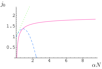
Figure 14: The pomeron intercept $j_{0}$ in ${\cal N}=4$ SYM as a function of the coupling $\alpha\,N$. The dotted line represents the perturbative LO BFKL pomeron intercept, the dashed line is the LO+NLO BFKL intercept, and the solid line is the strong-coupling AdS result. (The picture is taken from the talk by Tan.)

However, in a realistic high energy DIS scattering the incoming virtual photon splits into a quark–anti-quark pair very much in advance of the system hitting the proton or nuclear target. Hence a more realistic scenario would involve a finite-size medium, such that $L=2R$ with $R$ the radius of the target proton/nucleus. Then one gets $Q_{s}\sim R\,T^{2}$, i.e. the saturation scale is independent of Bjorken $x$, or, equivalently, of energy. In this regime the conclusions presented by Iancu agree with the results of other groups [62, 63]. It is rather interesting to observe that at large coupling the saturation scale becomes independent of energy. It seems that the classical super-gravity gives results similar to those given by the classical Yang-Mills fields in the McLerran-Venugopalan (MV) model [64]: there the saturation scale is also independent of energy. In the MV model we know that quantum corrections lead to energy-dependence of $Q_{s}$ [9, 10]. It is possible that quantum (order $1/\sqrt{\lambda}$) corrections in AdS would make the saturation scale energy-dependent at strong coupling.

AdS/CFT correspondence allows one to try to understand other related quantities, such as the intercept of the pomeron and the pomeron trajectory. The results of such investigations were presented by Tan. He explained how an AdS/CFT calculation gives the pomeron intercept $j_{0}=2-\frac{2}{\sqrt{\lambda}}$ for a strongly-coupled ${\cal N}=4$ SYM theory. His results are summarized in Fig. 14, where the intercept is plotted as a function of the gauge coupling $\alpha$ times the number of colors in the theory $N$. The dotted and dashed lines represent the perturbative LO and LO+NLO BFKL intercepts correspondingly. One can see that the NLO BFKL correction is indeed large and threatens to make the intercept less than 1 at not very large $\alpha\,N$. The solid line in Fig. 14 represents the AdS strong-coupling result of $j_{0}=2-\frac{2}{\sqrt{\lambda}}$: the picture suggests that an interpolation between the two results is possible, leading to an intercept which is greater than 1 at all values of the coupling.

At the same time I have to point out that the result of a recent AdS investigation [62] suggests that at high energies multiple exchanges of the intercept-2 pomerons lead to a somewhat unphysical behavior of the cross section and violate the black disk limit. In [62] an alternative solution was proposed with the strong coupling pomeron having an intercept of $j_{0}=1.5$ and with multiple exchanges of such a pomeron giving cross sections which are unitary and do not violate the black disk limit. More investigations may be needed to understand the differences between the two results.

Lipatov talked about another important result related to AdS/CFT correspondence — the BDS amplitude ansatz [65]. He has argued that the ansatz is violated in the Regge limit, when one calculates the diagrams contributing to the BFKL evolution. The violation is relatively minor and only manifests itself in some channels. This allows one to hope that a modification of the BDS ansatz is possible which would take into account the discrepancy presented by Lipatov.

9 Higgs boson and physics beyond the Standard Model

LHC had turned on just before the start of ISMD 2008, but had to be shut down soon after due to a malfunction of the superconducting magnets. Nevertheless, despite the delay, LHC era is upon us and a number of talks at ISMD 2008 were dedicated to what one could discover at LHC. While some aspects of the LHC heavy ion program have been mentioned above, here I will concentrate on the search for new particles in proton-proton collisions.

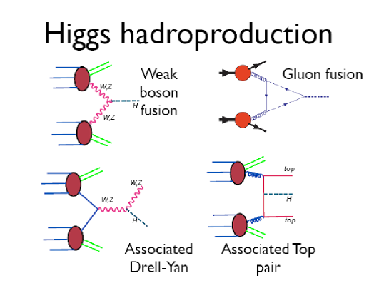
Figure 15: Various possible channels of Higgs boson production at LHC (from the talk by Anastasiou.)

First of all, if the Standard Model is correct, one expects to be able to find the Higgs boson at the LHC. Anastasiou gave a talk reviewing various channels of Higgs production, which are demonstrated in Fig. 15. Hopefully many (or at least one) of these channels would be observed at LHC.

It is possible however that backgrounds at LHC would be too high making the events shown in Fig. 15 hard to detect. In this case a possible cleaner signature of the Higgs would be the double diffraction production process illustrated in Fig. 16, which was discussed in the talks by Kaidalov and V. A. Khoze. In such process there will be rapidity gaps between the produced Higgs boson and each of the protons, allowing for a clean detection of the products of the Higgs boson decay, and thus for an unambiguous identification of the Higgs boson.

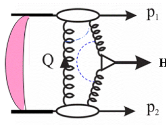
Figure 16: Double diffractive Higgs boson production mechanism at the LHC (from the talk by V.A. Khoze.)

Unfortunately, as often happens when the soft QCD interactions are involved, theoretical predictions for the cross sections of the process shown in Fig. 16 at LHC vary quite significantly [66, 67, 68]. Two of the existing approaches [67, 68] were reviewed in the talk by Kaidalov. Among other things he outlined the approximations made for the triple pomeron vertex made in each of the approaches. Both approaches reproduce the existing Tevatron double diffractive data reasonably well, but differ significantly in their extrapolation to LHC energies. Since it is not clear from first principles which approximation of the triple pomeron vertex is better justified, it seems that error analyses similar to those done for PDF’s may be needed to reconcile the differences between the two approaches in question.

Physics beyond the Standard Model was discussed in the talks by V.V. Khoze and Strassler dedicated to different supersymmetric models. While the former talk presented a minimal approach to introducing SUSY, the latter talk featured a broader range of possibilities. V.V. Khoze talked about the ISS scenario [69] in which the Universe lives in a metastable vacuum in which SUSY is broken. At the same time there exists a hidden sector of the theory with a true vacuum which is supersymmetric. The ISS model gives a concrete example of SUSY breaking, allowing to calculate the mass spectrum of the supersymmetric particles using the messenger fields. Strassler in his talk argued that minimalistic approach to physics beyond Standard Model is not necessarily what happens in nature and we should prepare for big surprises at the LHC. He therefore talked about hidden valleys and unparticles, both of which would lead to spectacular hadronic shower events at the LHC, which unfortunately would be hard to analyze and understand due to the large number of particles produced. Indeed both minimal and non-minimal SUSY scenarios are quite possible at LHC.

References

- [1] J. Jalilian-Marian and Y. V. Kovchegov, Prog. Part. Nucl. Phys. 56, 104 (2006). hep-ph/0505052
- [2] Y. L. Dokshitzer, Sov. Phys. JETP 46, 641 (1977)
- [3] V. N. Gribov and L. N. Lipatov, Sov. J. Nucl. Phys. 15, 438 (1972)
- [4] G. Altarelli and G. Parisi, Nucl. Phys. B126, 298 (1977)
- [5] Y. Y. Balitsky and L. N. Lipatov, Sov. J. Nucl. Phys. 28, 822 (1978)
- [6] E. A. Kuraev, L. N. Lipatov, and V. S. Fadin, Sov. Phys. JETP 45, 199 (1977)
- [7] J. Jalilian-Marian, A. Kovner, A. Leonidov, and H. Weigert, Phys. Rev. D59, 014014 (1998). hep-ph/9706377
- [8] E. Iancu, A. Leonidov, and L. D. McLerran, Nucl. Phys. A692, 583 (2001). hep-ph/0011241
- [9] I. Balitsky, Nucl. Phys. B463, 99 (1996). hep-ph/9509348
- [10] Y. V. Kovchegov, Phys. Rev. D60, 034008 (1999). hep-ph/9901281
- [11] CTEQ Collaboration, H. L. Lai et al., Eur. Phys. J. C12, 375 (2000). hep-ph/9903282
- [12] A. D. Martin, W. J. Stirling, R. S. Thorne, and G. Watt, Phys. Lett. B652, 292 (2007). 0706.0459
- [13] S. Alekhin, Phys. Rev. D68, 014002 (2003). hep-ph/0211096
- [14] NNPDF Collaboration, R. D. Ball et al. (2008). 0808.1231
- [15] STAR Collaboration, S. Salur (2008). 0809.1609
- [16] PHENIX Collaboration, S. S. Adler et al., Phys. Rev. Lett. 91, 072303 (2003). nucl-ex/0306021
- [17] STAR Collaboration, J. Adams et al., Phys. Rev. Lett. 91, 072304 (2003). nucl-ex/0306024
- [18] BRAHMS Collaboration, I. Arsene et al., Phys. Rev. Lett. 91, 072305 (2003). nucl-ex/0307003
- [19] V. S. Fadin and L. N. Lipatov, Phys. Lett. B429, 127 (1998). hep-ph/9802290
- [20] M. Ciafaloni and G. Camici, Phys. Lett. B430, 349 (1998). hep-ph/9803389
- [21] J. R. Andersen and A. Sabio Vera, Nucl. Phys. B679, 345 (2004). hep-ph/0309331
- [22] M. Ciafaloni, D. Colferai, G. P. Salam, and A. M. Stasto, Phys. Rev. D68, 114003 (2003). hep-ph/0307188
- [23] G. Altarelli, R. D. Ball, and S. Forte, Nucl. Phys. B575, 313 (2000). hep-ph/9911273
- [24] D. Kharzeev, E. Levin, and L. McLerran, Phys. Lett. B561, 93 (2003). hep-ph/0210332
- [25] D. Kharzeev, Y. V. Kovchegov, and K. Tuchin, Phys. Rev. D68, 094013 (2003). hep-ph/0307037
- [26] J. L. Albacete, N. Armesto, A. Kovner, C. A. Salgado, and U. A. Wiedemann, Phys. Rev. Lett. 92, 082001 (2004). hep-ph/0307179
- [27] BRAHMS Collaboration, I. Arsene et al., Phys. Rev. Lett. 93, 242303 (2004). nucl-ex/0403005
- [28] PHENIX Collaboration, S. S. Adler et al., Phys. Rev. Lett. 94, 082302 (2005). nucl-ex/0411054
- [29] PHOBOS Collaboration, B. B. Back et al., Phys. Rev. C70, 061901 (2004). nucl-ex/0406017
- [30] STAR Collaboration, J. Adams et al., Phys. Rev. Lett. 97, 152302 (2006). nucl-ex/0602011
- [31] K. J. Eskola, H. Paukkunen, and C. A. Salgado, JHEP 07, 102 (2008). 0802.0139
- [32] Y. V. Kovchegov and K. Tuchin, Phys. Rev. D65, 074026 (2002). hep-ph/0111362
- [33] D. Kharzeev, E. Levin, and M. Nardi, Phys. Rev. C71, 054903 (2005). hep-ph/0111315
- [34] J. L. Albacete, Phys. Rev. Lett. 99, 262301 (2007). 0707.2545
- [35] Y. V. Kovchegov and H. Weigert, Nucl. Phys. A784, 188 (2007). hep-ph/0609090
- [36] I. Balitsky, Phys. Rev. D75, 014001 (2007). hep-ph/0609105
- [37] J. L. Albacete and Y. V. Kovchegov, Phys. Rev. D75, 125021 (2007). 0704.0612
- [38] STAR Collaboration, M. Daugherity, J. Phys. G35, 104090 (2008). 0806.2121
- [39] J. Casalderrey-Solana, E. V. Shuryak, and D. Teaney, J. Phys. Conf. Ser. 27, 22 (2005). hep-ph/0411315
- [40] PHENIX Collaboration, A. Adare et al., Phys. Rev. C77, 011901 (2008). 0705.3238
- [41] A. Kovner and U. A. Wiedemann, Phys. Lett. B551, 311 (2003). hep-ph/0207335
- [42] T. Lappi and L. McLerran, Nucl. Phys. A772, 200 (2006). hep-ph/0602189
- [43] S. Mrowczynski, Phys. Lett. B314, 118 (1993)
- [44] P. Arnold, J. Lenaghan, and G. D. Moore, JHEP 08, 002 (2003). hep-ph/0307325
- [45] A. Kovner, L. D. McLerran, and H. Weigert, Phys. Rev. D52, 6231 (1995). hep-ph/9502289
- [46] Y. V. Kovchegov and D. H. Rischke, Phys. Rev. C56, 1084 (1997). hep-ph/9704201
- [47] A. Krasnitz, Y. Nara, and R. Venugopalan, Nucl. Phys. A727, 427 (2003). hep-ph/0305112
- [48] Y. V. Kovchegov and H. Weigert, Nucl. Phys. A807, 158 (2008). 0712.3732
- [49] J. M. Maldacena, Adv. Theor. Math. Phys. 2, 231 (1998). hep-th/9711200
- [50] E. Witten, Adv. Theor. Math. Phys. 2, 253 (1998). hep-th/9802150
- [51] R. A. Janik and R. B. Peschanski, Phys. Rev. D73, 045013 (2006). hep-th/0512162
- [52] J. D. Bjorken, Phys. Rev. D27, 140 (1983)
- [53] L. D. Landau, Izv. Akad. Nauk SSSR Ser. Fiz. 17, 51 (1953)
- [54] BRAHMS Collaboration, I. G. Bearden et al., Phys. Rev. Lett. 93, 102301 (2004). nucl-ex/0312023
- [55] P. Huovinen, P. F. Kolb, U. W. Heinz, P. V. Ruuskanen, and S. A. Voloshin, Phys. Lett. B503, 58 (2001). hep-ph/0101136
- [56] D. Teaney, J. Lauret, and E. V. Shuryak (2001). nucl-th/0110037
- [57] G. Policastro, D. T. Son, and A. O. Starinets, Phys. Rev. Lett. 87, 081601 (2001). hep-th/0104066
- [58] P. Kovtun, D. T. Son, and A. O. Starinets, Phys. Rev. Lett. 94, 111601 (2005). hep-th/0405231
- [59] M. A. Lisa and S. Pratt (2008). 0811.1352
- [60] Y. V. Kovchegov and A. Taliotis, Phys. Rev. C76, 014905 (2007). 0705.1234
- [61] O. Aharony, S. S. Gubser, J. M. Maldacena, H. Ooguri, and Y. Oz, Phys. Rept. 323, 183 (2000). hep-th/9905111
- [62] J. L. Albacete, Y. V. Kovchegov, and A. Taliotis, JHEP 07, 074 (2008). 0806.1484
- [63] F. Dominguez, C. Marquet, A. H. Mueller, B. Wu, and B.-W. Xiao, Nucl. Phys. A811, 197 (2008). 0803.3234
- [64] L. D. McLerran and R. Venugopalan, Phys. Rev. D49, 2233 (1994). hep-ph/9309289
- [65] Z. Bern, L. J. Dixon, and V. A. Smirnov, Phys. Rev. D72, 085001 (2005). hep-th/0505205
- [66] J. Bartels, S. Bondarenko, K. Kutak, and L. Motyka, Phys. Rev. D73, 093004 (2006). hep-ph/0601128
- [67] E. Gotsman, E. Levin, U. Maor, and J. S. Miller (2008). 0805.2799
- [68] V. A. Khoze, A. D. Martin, and M. G. Ryskin, Phys. Lett. B650, 41 (2007). hep-ph/0702213
- [69] K. A. Intriligator, N. Seiberg, and D. Shih, JHEP 04, 021 (2006). hep-th/0602239.