Stationary waves in a supersonic flow of a two-component Bose gas

Abstract

A stationary wave pattern occurring in a flow of a two-component Bose-Einstein condensate past an obstacle is studied. We consider the general case of unequal velocities of two superfluid components. The Landau criterium applied to the two-component system determines a certain region in the velocity space in which superfluidity may take place. Stationary waves arise out of this region, but under the additional condition that the relative velocity of the components does not exceed some critical value. Under increase of the relative velocity the spectrum of the excitations becomes complex valued and the stationary wave pattern is broken. In case of equal velocities two sets of stationary waves that correspond to the lower and the upper Bogolyubov mode can arise. If one component flows and the other is at rest only one set of waves may emerge. Two or even three interfere sets of waves may arise if the velocities approximately of equal value and the angle between the velocities is close to $\pi/2$. In two latter cases the stationary waves correspond to the lower mode and the densities of the components oscillate out-of-phase. The ratio of amplitudes of the components in the stationary waves is computed. This quantity depends on the relative velocity, is different for different sets of waves, and varies along the crests of the waves. For the cases where two or three waves interfere the density images are obtained.

1 Introduction

A unique feature of two-component Bose-Einstein condensates (BEC) is the possibility for two superfluids to flow with different velocities. The properties of such systems can be described by the three-velocity hydrodynamics (one normal and two superfluid velocities). This feature was already noticed by Khalatnikov hal . The modern three-velocity superfluid hydrodynamic theory was formulated in the paper by Andreev and Bashkin ab . As was shown in ab the specifics of the three-velocity superfluid hydrodynamics is the presence of a non-dissipative drag between the components. The drag effect emerges at nonzero relative velocity of the components and consists in a dependence of the superfluid current of one component on the gradient of the phase of the order parameter of the other component. The microscopic theory of the non-dissipative drag effect was developed in fil1 ; fil . An important question that arises in the three-velocity superfluid hydrodynamics is the question on critical velocities. At equal velocities of the components the answer to this question can be obtained from the Galilean transformation. It yields that under neglecting of vortex excitations the critical velocity coincides with the minimal phase velocity of the lower Bogolyubov mode. In a wider sense one can introduce two critical velocities $c_{-}$ and $c_{+}$, one is for the lower mode and the other is for the upper mode nb ; bi2 .

In case of unequal velocities of the components the situation becomes more complicated. The question was considered in Refs. yukalov ; 6 . The authors of yukalov have obtained the dispersion equation for the spectrum of elementary excitations in the presence of superfluid flows. However the analysis of critical velocities in yukalov was based on the implication that the Landau criterium can be formulated as the condition on the relative velocity of the superfluid components. Such an implication can be put in question since there are two independent relative velocities in the three-velocity theory. In 6 the Landau criterium was formulated as the condition of positiveness of energies of elementary excitations in a reference frame connected with a normal component. It yields a joint condition on absolute values of the superfluid velocities of the components and on the angle between their directions. If one component is at rest the superfluidity condition 6 is reduced to yukalov .

The analysis carried out in 6 shows that the Landau criterium may be fulfilled if one or even both superfluid velocities exceed the velocity of the lower mode $c_{-}$(in the latter case the velocities should have different directions). In view of unusual behaviour of critical velocities in such systems it is interesting to consider how this behavior can reveal itself in experiments. Two-component BECs have been realized experimentally in ultracold alkali metals gases confined in magnetic and magneto-optical traps. Two components may correspond to different hyperfine Zeeman states of the same isotope Rb2 ; Rb-n , or to different isotopes K-Rb ; K-Rb1 ; Rb3 . One of the methods to determine critical velocities for trapped ultracold gases consists in the observation of density excitations induced by some object moving through the condensate exp (usually a laser beam is used as such an object). A motion of an object in a two-component gas with nonzero relative velocity of the superfluid components corresponds to the general case of the three-velocity hydrodynamics.

The Bogolyubov spectrum has a dispersion. Therefore, a motion of an object through a superfluid system (or a superfluid flow past an obstacle) can lead to an occurrence of stationary waves (the waves whose crests remain at rest relative to the obstacle). Such an effect called ”ship waves” is well-known wi . It was considered by Kelvin for the waves generated on a water surface by a ship moving in a deep water. Stationary waves in a one-component quasi-two-dimensional BEC were studied in ship . It was shown that in a superfluid that flows past a point obstacle (the obstacle size is less than the healing length) the stationary wave pattern is similar to one for stationary capillary waves. The effect takes place if the superfluid velocity $s$ exceeds the minimal phase velocity of the Bogolyubov mode $c_{0}$. The stationary waves arise outside the Mach cone bounded by arms directed at the angles $\vartheta=\pm\arcsin(c_{0}/s)$ relative to the flow.

In recent papers the solitons bi2 ; 16 and stationary waves 16 induced by an obstacle in a two-component superfluid system were studied (the paper 16 was published as the electronic preprint when the present study was almost completed). But the authors of bi2 ; 16 considered only the case of equal superfluid velocities (a relative velocity of the components is equal to zero).

In the present paper we put emphasis on the general case of nonzero relative velocity. In Sec. 2 we obtain the equation for the spectrum and the eigenvectors of collective excitations and define two more critical velocities (in addition to $c_{-}$ and $c_{+}$). One of them is the maximum critical velocity $c_{m}$ for a given component ($c_{m}>c_{-}$). The superflow at the velocity $s\to c_{m}$ can be reached if the other component is at rest. The other is the relative critical velocity $c_{\rm sep}$ ($c_{\rm sep}>c_{m}$). If the relative velocity exceeds $c_{\rm sep}$, the frequency of the lower mode becomes complex valued. The latter signals for an instability of the two-component system with respect to a spatial separation of the components. In Sec.3 the equation that describes the stationary wave pattern is obtained. It is shown that the stationary waves emerge if the Landau criterium of superfluidity is violated (the energies of the excitations with certain wave vectors becomes negative), but the system remains stable with respect to the spatial separation (the critical relative velocity is not achieved). A number of stationary wave patterns are presented. It is shown that depending on the velocities of the components several qualitatively different situations are possible. If the velocities are the same in modulus and in direction, one set of stationary waves appears at $s>c_{-}$, and another set adds at $s>c_{+}$. The phase separation does not occur. If only one component moves with the velocity $s$, one set of stationary waves is formed at $s>c_{m}$ but if $s$ reaches $c_{\rm sep}$ the phase separation occurs. If the velocities are equal in modulus and the angle between their directions is $\pi/2$ or close to $\pi/2$ two or three sets of stationary waves occur at $s_{1}=s_{2}>c_{m}$. In Sec. 4 we investigate the structure of the stationary waves. The densities of the components always oscillate out-of-phase in the waves that correspond to the lower mode . The ratio of the amplitudes of the oscillations of the components depends on the relative velocity and varies along the crests of the waves. For complex density patterns where two or three waves interfere the density plots are presented. It is established that the stationary waves are visible in total density images as well as relative density images, but in most cases relative density images are more contrast. The only exception is the stationary waves that are exited at $s>c_{+}$ and correspond to the upper Bogolyubov mode.

2 The spectrum of collective modes

To analyze the stationary waves in a two-component superfluid system one should obtain the collective modes spectrum in a moving condensate. It can be found from the matrix version of the Gross-Pitaevskii equation

$$i\hbar\frac{\partial\psi_{1}}{\partial t}=-\frac{\hbar^{2}}{2m_{1}}\triangle\psi_{1}+\gamma_{1}|\psi_{1}|^{2}\psi_{1}+\gamma_{12}|\psi_{2}|^{2}\psi_{1},$$ (1)

$$i\hbar\frac{\partial\psi_{2}}{\partial t}=-\frac{\hbar^{2}}{2m_{2}}\triangle\psi_{2}+\gamma_{2}|\psi_{2}|^{2}\psi_{2}+\gamma_{12}|\psi_{1}|^{2}\psi_{2},$$ (2)

where $\psi_{i}$ are the wave functions of the components, $m_{i}$ are the masses of the particles,

$$\gamma_{i}=\frac{4\pi\hbar^{2}a_{i}}{m_{i}},\;\gamma_{12}=\frac{2\pi\hbar^{2}(m_{1}+m_{2})a_{12}}{m_{1}m_{2}}$$ (3)

are the interaction constants ($a_{i}$ and $a_{12}$ are scattering lengthes).

Here we restrict the consideration by the most convenient for the analysis symmetric case for which the components have equal masses of the particles $m_{1}=m_{2}=m$, equal densities $n_{1}=n_{2}=n_{0}$ of the components and equal interaction constants $\gamma_{1}=\gamma_{2}=\gamma$. While this case is quite specific, it is possible to produce equal $\gamma_{i}$ using a Feshbach resonance. The symmetric case may also correspond to two quasi two-dimensional Bose clouds with a strong dipole interaction separated by a rather high (but thin) barrier that suppress the tunneling (see fil1 ). On the qualitative level the results obtained for the symmetric case hold for the general case where such a symmetry between the components is broken. We assume the interaction between the particles of the same component is repulsive ($\gamma>0$), and the stability condition with respect to a spatial separation of the components $(\gamma>|\gamma_{12}|)$ is fulfilled. Going ahead we note that in case of different velocities that condition is necessary but not sufficient one.

If the temperature is much less than the temperature of the Bose-Einstein condensation the wave functions of the components can be presented as a sum of a large stationary part and a small fluctuating part

$$\psi_{i}(\mathbf{r},t)=\psi_{0i}(\mathbf{r},t)+\delta\psi_{i}(\mathbf{r},t).$$ (4)

The stationary part of the condensate wave function reads as

$$\psi_{0i}(\mathbf{r},t)=\sqrt{n_{0}}\,e^{i\varphi_{i}(\mathbf{r})}e^{-\frac{i\mu_{i}t}{\hbar}},$$ (5)

where $\mu_{i}=\displaystyle\frac{m_{i}\mathbf{s}_{i}^{2}}{2}+(\gamma+\gamma_{12})n_{0}$ are the chemical potentials of the components, and $\mathbf{s}_{j}=\displaystyle\frac{\hbar}{m}\nabla\varphi_{j}$ are their superfluid velocities. We will search for the fluctuating part of Eq. (4) in the form:

$$\delta\psi_{i}(\mathbf{r},t)=e^{i\varphi_{i}(\mathbf{r})}e^{-\frac{i\mu_{i}t}{\hbar}}\left[\textrm{u}_{i}(\mathbf{r})e^{-i\omega t}+\textrm{v}_{i}^{*}(\mathbf{r})e^{i\omega^{*}t}\right].$$ (6)

Here the functions $\textrm{u}_{i}$ and $\textrm{v}_{i}$ are the plane waves

$$\textrm{u}_{i}(\mathbf{r})=A_{i}e^{i\mathbf{k}\mathbf{r}},\;\textrm{v}_{i}(\mathbf{r})=B_{i}e^{i\mathbf{k}\mathbf{r}}.$$ (7)

Substituting Eqs. (4) – (7) into Eq. (1), in a linear in fluctuations approximation we obtain the following equation for the excitation energies $\hbar\omega$ and the eigenvectors:

$$\mathbf{M}\mathbf{V}=\omega\mathbf{V},$$ (8)

where

$$\mathbf{M}=\left(\begin{array}[]{cccc}\displaystyle\left(\frac{k^{2}}{2}+1+\mathbf{s}_{1}\mathbf{k}\right)&1&\gamma^{\prime}&\gamma^{\prime}\\ -1&\displaystyle-\left(\frac{k^{2}}{2}+1-\mathbf{s}_{1}\mathbf{k}\right)&-\gamma^{\prime}&-\gamma^{\prime}\\ \gamma^{\prime}&\gamma^{\prime}&\displaystyle\left(\frac{k^{2}}{2}+1+\mathbf{s}_{2}\mathbf{k}\right)&1\\ -\gamma^{\prime}&-\gamma^{\prime}&-1&\displaystyle-\left(\frac{k^{2}}{2}+1-\mathbf{s}_{2}\mathbf{k}\right)\\ \end{array}\right)$$ (9)

and

$$\mathbf{V}=\left(\begin{array}[]{c}A_{1}\\ B_{1}\\ A_{2}\\ B_{2}\\ \end{array}\right)$$ (10)

Here and below all physical quantities are expressed in terms of dimensionless length and time

$$\tilde{r_{i}}=\frac{r_{i}}{\sqrt{2}\xi},\;\tilde{t}=\frac{c_{0}}{\sqrt{2}\xi}t,$$ (11)

where $c_{0}=\sqrt{\gamma n_{0}/m}$ is a sound velocity in a one-component condensate, and $\xi=\hbar/\sqrt{2m\gamma n_{0}}$ is a healing length. We also define the dimensionless parameter of the interspecie interaction $\gamma^{\prime}=\gamma_{12}/\gamma$.

The $u-v$ transformation procedure (6) is equivalent to the diagonalization of a quadratic form on Bose operators pit ; bogol . The matrix $\mathbf{M}$ has four eigenvalues. The components of the eigenvectors of Eq. (8) can be normalized as $|A_{1}|^{2}-|B_{1}|^{2}+|A_{2}|^{2}-|B_{2}|^{2}=\pm 1/V$ ($V$ is the volume of the system). For two physical modes the norm of the eigenvector should be positive bogol . The spectra of the physical modes read as

$$\omega_{\pm}=\frac{(\mathbf{s}_{1}+\mathbf{s}_{2})\mathbf{k}}{2}+\sqrt{k^{2}\left(1+\frac{k^{2}}{4}\right)+\frac{(\mathbf{s}_{-}\mathbf{k})^{2}}{4}\pm\sqrt{k^{2}\left(1+\frac{k^{2}}{4}\right)(\mathbf{s}_{-}\mathbf{k})^{2}+k^{4}\gamma^{\prime 2}}},$$ (12)

where $\mathbf{s}_{-}=\mathbf{s}_{1}-\mathbf{s}_{2}$ is the relative superfluid velocity. At $s_{1}=s_{2}=0$ the spectrums (12) has the standard Bogolyubov form

$$\omega_{\pm}=k\sqrt{1\pm|\gamma^{\prime}|+k^{2}/4}.$$ (13)

As is clear from Eq. (13), the stability condition with respect to a spatial separation $\gamma>|\gamma_{12}|$ is the requirement for the excitation spectrum be real valued. At small $\mathbf{k}$ the excitation spectrum is a sound one and the velocities of the modes are equal to $c_{\pm}=\sqrt{1\pm|\gamma^{\prime}|}$. The Landau criterium requires the spectrum (12) be positive valued at all wave vectors. One can see from Eq.(12) that at $\mathbf{s}_{1}=\mathbf{s}_{2}=\mathbf{s}$ the Landau criterium is reduced to the inequality $s<c_{-}$. If only one component flows ($s_{2}=0$), the Landau criterium requires a fulfilment of the inequality $s_{1}<c_{m}=c_{-}\sqrt{1+|\gamma^{\prime}|}$. If the velocity of a given component exceeds $c_{m}$, the superfluidity condition is broken irrespective of a value and direction of the velocity of the other component 6 , i.e. $c_{m}$ can be called the maximum critical velocity.

At the velocities for which the energy (12) is negative valued in some range of ${\bf k}$ the Landau criterium is broken and stationary waves can occur in the system. In contrast to a one-component system, in a two-component system an increase of superfluid velocities may result in that the spectrum of the lower mode be complex valued. As follows from Eq. (12), the spectrum remains real valued if the relative velocity satisfies the condition

$$|\mathbf{s}_{1}-\mathbf{s}_{2}|<c_{\rm sep}=2c_{-}.$$ (14)

At complex valued frequencies (12) the amplitude of excitations grows with time that leads to a destruction of a homogeneous state and to a spatial separation of the components (or stratification). In contrast to Ref. yukalov , we consider the condition of stratification and the Landau criterium as different conditions. The Landau criterium yields a joint restriction on both superfluid velocities (and its mutual direction), while the condition of stratification is a restriction only on the modulus of the relative velocity. Note that $c_{\rm sep}>c_{m}$, and under increase of the velocity of a given component, first, the Landau criterium is violated, and then, after further increase, the stability condition with respect to the stratification is broken. One can show, that the same situation takes place under simultaneous increase of two velocities (at nonzero relative velocity). Only at equal in value and oppositely directed superfluid velocities the Landau criterium and the stability condition are broken at the same point.

Since we are interested in stationary waves in a homogeneous (not stratified) system, we will consider only the velocities for which the condition (14) is satisfied.

3 The stationary wave pattern

Let us consider a two-component BEC that flows past an obstacle situated at the origin of coordinates. We assume the system is quasi-two-dimensional, i.e. it is thin enough to neglect the dependence of the condensate wave function on the transverse coordinate, and to consider all vector quantities as two-dimensional ones. If the size of an obstacle is much less than $\xi$ it can be considered as a point one. Under violation of the Landau criterium the obstacle behaves as a point source of waves (below we are only interested in stationary waves). The waves propagate from an obstacle with the group velocities $\mathbf{v}_{g\pm}=\partial\omega_{\pm}/\partial\mathbf{k}$, where $\omega_{\pm}=\omega_{\pm}(k_{x},k_{y})$ are given by Eq. (12) at $k_{z}=0$. Here and below the index $+(-)$ corresponds to the waves generated by the upper (lower) mode. The direction of the propagation for the wave with a given $\mathbf{k}$ is defined by the expression

$$\tan\chi_{\pm}=\frac{\partial\omega_{\pm}/\partial k_{y}}{\partial\omega_{\pm}/\partial k_{x}},$$ (15)

where $\chi_{+}(\chi_{-})$ is the angle between the group velocity direction for a given mode and the axis $x$.

For the stationary wave the frequency (12) is equal to zero, and the components of the wave vector $\mathbf{k}=(k_{x},k_{y})$ are related by the equation

$$\omega_{\pm}(k_{x},k_{y})=0.$$ (16)

It is convenient to use the angle $\eta$ between the wave vector and the opposite direction of the axis $x$ as an independent parameter, i.e.

$$\mathbf{k}=(-k\cos\eta,k\sin\eta).$$ (17)

Let us denote the angle between the velocities by $\theta$ and select the axis $x$ along the bisectrix of this angle ($\mathbf{s}_{1}=(s_{1}\cos\frac{\theta}{2},-s_{1}\sin\frac{\theta}{2})$ and $\mathbf{s}_{2}=(s_{2}\cos\frac{\theta}{2},s_{2}\sin\frac{\theta}{2})$). For the stationary waves Eq. (16) yields the following dependence of the wave number $k$ on the angle $\eta$

$$\begin{array}[]{c}k_{\pm}(\eta)=\sqrt{2}\biggl{[}-2+s_{1}^{2}\cos^{2}\left(\eta-\frac{\theta}{2}\right)+s_{2}^{2}\cos^{2}\left(\eta+\frac{\theta}{2}\right)\mp\\ \left.\sqrt{4\gamma^{\prime 2}+\left(s_{1}^{2}\cos^{2}\left(\eta-\frac{\theta}{2}\right)-s_{2}^{2}\cos^{2}\left(\eta+\frac{\theta}{2}\right)\right)^{2}}\right]^{1/2}.\\ \end{array}$$ (18)

A wave crest line is a line of a constant phase. For the stationary wave the phase can be obtained from the equation

$$\phi(\mathbf{r})=\int_{0}^{\mathbf{r}}\mathbf{k}d\mathbf{r}.$$ (19)

In Eq. (19) the integral is along a straight line going out from the origin of coordinates and directed parallel to the group velocity $\mathbf{v}_{g\pm}$. The angle $\mu$ between $\bf{k}$ and $\bf{r}$ is defined by the expression

$$\mu=\pi-\eta-\chi_{\pm}$$ (20)

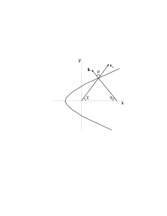
Figure 1: The scheme of a wavefront crest

(see Fig. 1).

According to Eq.(19), the quantity $r$ for the points at the wave crest with a given phase $\phi$ satisfies the equation

$$r=\frac{\phi}{k\cos\mu}.$$ (21)

Substituting Eq. (20) into Eq. (21), we get the equations for the stationary wave crest coordinates $x=r\cos\chi$ and $y=r\sin\chi$ in a parametric form

$$x_{\pm}=-\frac{\phi}{k_{\pm}(\eta)\cos\eta\left[1-\tan\chi_{\pm}\tan\eta\right]},$$ (22)

$$y_{\pm}=-\frac{\phi\tan\chi_{\pm}}{k_{\pm}(\eta)\cos\eta\left[1-\tan\chi_{\pm}\tan\eta\right]}.$$ (23)

In Eq. (22) the values $\tan\chi_{\pm}$ are the functions of the parameter $\eta$. The explicit form of these functions is given by Eq. (15), in which after differentiation one should substitute Eqs. (17) and (18). The range of values of $\eta$ is determined by the condition for the function $k_{\pm}(\eta)$ be real valued. Eqs. (22) allow to draw the stationary wave pattern for arbitrary values of $s_{1}$, $s_{2}$ and $\theta$.

Let us consider some special cases. For definiteness, we choose the parameter $\gamma^{\prime}=0.5$. Such a choice corresponds to $c_{-}=0.707$, $c_{m}=0.866$ and $c_{+}=1.22$ (in $c_{0}$ units).

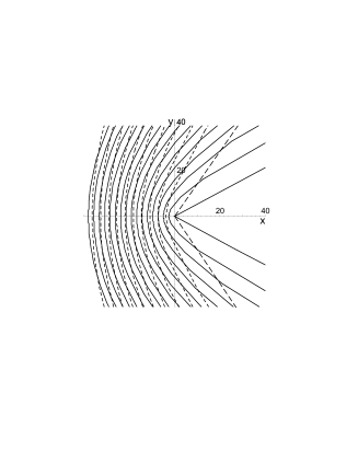
Figure 2: The wave pattern forming at the flow of components with equal velocities $(s=1.5)$. The waves caused by the lower and the upper modes are shown with solid and dashed lines, respectively.

1. At equal superfluid velocities $\mathbf{s}_{1}=\mathbf{s}_{2}=\mathbf{s}$ Eqs. (22) yield the expected result. At $s>c_{-}$ a set of stationary waves corresponding to the lower mode arises. The crests for these waves are outside the cone bounded by the arms $\chi_{1}=\pm\arcsin(c_{-}/s)$. If the velocities $s>c_{+}$ are reached the second set of stationary waves appears. It corresponds to the upper mode and situated outside the arms $\chi=\pm\arcsin(c_{+}/s)$. Since $s_{-}=0$, the stratification does not occur at any $s$. As an example, the stationary wave pattern for $s=1.5$ is shown in Fig.2.

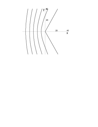
Figure 3: The wave pattern forming at the flow of one component with the velocity $s_{1}=1.0\,(s_{2}=0)$. The axis $x$ is along the flow direction.

2. If only one component (say, the component 1) flows, the stationary waves arise at the velocities $s_{1}>c_{m}$. These waves correspond to the lower mode. The waves are outside the cone $\chi_{-}=\pm\arcsin(c_{m}/s)$. In this case the frequency of the upper mode is always positive and the second set of waves cannot arise. At $s_{1}>c_{\rm sep}$ (for the parameters chosen $c_{\rm sep}=1.41$) the system becomes unstable with respect to the stratification. The stationary wave pattern for the flow of one component with $s_{1}=1.0$ is shown in Fig.3.

3. It is interesting to analyze the situation when the angle between the velocities is $\theta=\pi/2$. In this case the obstacle emits waves only when the velocity of at least one component exceeds $c_{m}$. Let us consider a more specific case of the velocities equal in magnitude $s_{1}=s_{2}=s$. Then the velocity range in which the stationary waves occur is limited by the condition $c_{m}<s<\sqrt{2}c_{-}$ (for the parameters chosen $0.866<s<1$). In Fig.4 we present the stationary wave pattern for $s=0.9$. One can see that in such a situation two sets of stationary waves arise. It is important to emphasize that both sets correspond to the lower mode (the frequency of the upper mode remains positive for the velocities in the range $c_{m}<s<\sqrt{2}c_{-}$).

In the limit $\gamma^{\prime}\to 0$ (that corresponds to the absence of the interaction between the components) each component should have its own set of stationary waves at any relative directions of the velocities. For rather large $\gamma^{\prime}$ this feature survives only in a close vicinity to $\theta=\pi/2$. There should be a smooth transition from $\theta=\pi/2$ to $\theta=0$. The analysis of the wave patterns at different $\theta$ shows that at intermediate $\theta$ a quite complicated pattern emerges: the crests of a given set end with cusps, and bridges connect them with crests from the other set. Under decrease of $\theta$ the bridges and cusps disappear and the wave pattern becomes similar to one for $\theta=0$. The stationary wave pattern with cusps and bridges is shown in Fig. 5.

In general, the stationary wave pattern is qualitatively similar to one of presented in Figs. 2-5.

4 The density pattern for the stationary waves

There is a number of methods of probing BECs to get their density profiles (see ket ). Advanced technics was developed for the study of density profiles of spinor BECs c0 ; c1 ; c2 ; c3 ; prl05 (that in certain sence can be considered as two-component ones). In particular, the density and the spin-density profiles of an atomic cloud were measured with a high resolution by the polarization-dependent phase-contrast imaging method prl05 ; sk07 .

In view of modern experimental possibilities it is important to find the ratio of the components in the stationary waves and to determine specific features of the total density and the relative density patterns for the stationary wave in two-component systems.

Since the stationary wave is the eigenmode, the ratio of the total density and relative density amplitudes can be found from the corresponding eigenvector (10).

The density of a given component is the square modulus of the condensate wave function $\rho_{i}=|\psi_{i}|^{2}$. This quantity can be presented as a sum of the unperturbed density $n_{0}$ and the perturbation $\delta n_{i}$ caused by the stationary wave. Using the equation for the condensate wave function (4) and Eqs. (5) – (7), we obtain

$$\delta n_{i}=\psi_{0}\delta\psi_{i}^{*}+\delta\psi_{i}\psi_{0}^{*}=\delta\rho_{i}\cos(\mathbf{k}\mathbf{r}),$$ (24)

where

$$\delta\rho_{i}={\cal A}\sqrt{n_{0}}(A_{i}+B_{i}).$$ (25)

here ${\cal A}$ is the amplitude of a given eigenmode. The amplitude ${\cal A}$ depends on the intensity of the source (obstacle) and on the distance from the source. As follows from Eqs. (8,9), the components of the eigenvectors are real valued quantities. That is why Eq. (25) may correspond to in-phase oscillations of the densities or to the oscillation with the phase shift equal to $\pi$ (out-of-phase). Here we consider the case $\gamma^{\prime}>0$ for which the lower Bogolyubov mode corresponds to out-of-phase oscillations and the higher mode - to in-phase oscillations.

The total density and the relative density oscillation amplitudes in the stationary wave are $\delta\rho_{\pm}=\rho_{1}\pm\rho_{2}$. The specific of the symmetric case (components with equal masses, densities and interaction constants) is that in the absence of the flow the oscillations of the total density vanish for the lower Bogolyubov mode ($\delta\rho_{+}=0$), and the oscillations of the relative density are absent in the higher mode ($\delta\rho_{-}=0$). As was shown in the previous section, in most cases the stationary waves are caused by the lower mode. Therefore it is important to clarify whether is the total density disturbed in the stationary waves.

Using the analytical expressions for the eigenvectors of the matrix (9) one finds that the exact relations $\delta\rho_{1}=-\delta\rho_{2}$ for the lower mode and $\delta\rho_{1}=\delta\rho_{2}$ for the upper mode are hold in case of equal velocities (${\bf s}_{1}={\bf s}_{2}$). In means that in the stationary wave pattern shown in Fig. 2 the lower mode set is visible in the relative density image, while the upper mode set - in the total density image.

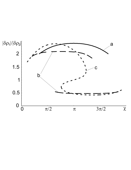
Figure 6: The ratio of densities of the components in the stationary waves along the chests for: a) one component flow $(s_{1}=1,s_{2}=0)$; b) two component flow in mutually orthogonal directions $(\theta=\pi/2,s_{1}=s_{2}=0.9)$; c) the case of $\theta=0.45\pi,s_{1}=s_{2}=1$.

In the general case ${\bf s}_{1}\neq{\bf s}_{2}$ we find that $\delta\rho_{1}\neq-\delta\rho_{2}$ and the total density oscillations are nonzero for the stationary waves that correspond to the lower mode, in particular, for the pattern shown in Figs. 3 - 5. For these cases the ratios $|\delta\rho_{1}|/|\delta\rho_{2}|$ along the crests are shown in Fig. 6. Since this ratio differs from unity, both, $\delta\rho_{+}$ and $\delta\rho_{-}$ are nonzero and stationary wave patterns should be visible in the total density image as well as in the relative density image. We also would like to point out the feature that follows from Fig. 6. If only one component flows past the obstacle the stationary waves contain admixture of both components, but the flowing component has larger amplitude.

In cases shown in Figs. 3,4 two or three sets of stationary waves interfere. Thus the density pattern depends not only on the eigenvectors but on the amplitudes of the eigenmodes, and another approach should be used to analyze the density profiles. Here we use the approach developed in 16 .

The interaction of the Bose gas with the obstacle is described by the Hamiltonian

$$H_{int}=\int d{\bf r}\sum_{i}V_{i}(\mathbf{r})|\psi_{i}|^{2},$$

where $V_{i}(\mathbf{r})$ is the potential of the interaction between the $i$-th component and the obstacle. Considering the obstacle as a point source and assuming that the obstacle interacts identically with both components we set $V_{1}(\mathbf{r})=V_{2}(\mathbf{r})=V_{0}\delta({\bf r})$. Respectively, the terms $V_{0}\delta({\bf r})\psi_{i}$ should be added to the right hand parts of the Gross-Pitaevskii equations (1). The Gross-Pitaevskii equations can be rewritten in terms of density and velocity fields (the hydrodynamic form). Linearizing the hydrodynamic equations with respect to the density and velocity fluctuations (see, for instance, 6 ), and excluding the velocity fluctuations we arrive at the equations for the Fourier components of $\delta n_{i}$:

$$\left[-\left(\mathbf{s}_{i}\mathbf{k}\right)^{2}+k^{2}\left(1+\frac{k^{2}}{4}\right)\right]\delta n_{i}({\bf k})+k^{2}\gamma^{\prime}\delta{n}_{3-i}({\bf k})=-k^{2}\tilde{V}_{0},$$ (26)

where $\tilde{V}_{0}=V_{0}/\gamma$. In deriving Eq. (26) we take into account that all time derivatives are zero for the stationary waves.

Solving Eq.(26) and taking the inverse Fourier transformation we get

$$\delta n_{i}=-\frac{4V_{0}}{\pi^{2}\gamma\xi^{2}}{\rm Re}\int_{-\pi/2}^{\pi/2}d\eta\int_{0}^{\infty}kdk\frac{1-\gamma^{\prime}+\frac{k^{2}}{4}-\frac{\left(\mathbf{s}_{i}\mathbf{k}\right)^{2}}{k^{2}}}{(k^{2}-k_{+}^{2})(k^{2}-k_{-}^{2})}\,e^{ikr\cos\mu},$$ (27)

where the quantities $k_{\pm}$ are given by Eq. (18). The angle $\mu(\eta)$ is determined by Eqs. (20) and (15). The integral over $k$ in Eq.(27) can be evaluated analytically with the use of the residue theorem. The poles $k=k_{-}$ and $k=k_{+}$ (for real $k_{\pm}$) yield the contribution of the lower and the upper Bogolyubov modes, respectively. The integral over $\eta$ is evaluated by the stationary phase method. The number of stationary phase points coincides with the number interfered waves in the stationary wave pattern (1 point for Figs. 2 and 3, 2 points for Fig. 4 and 3 points for Fig. 5).

The answer can be presented in the following form

$$\delta n_{i}\approx\frac{V_{0}}{\gamma\xi^{2}}\sum_{i,\lambda}C_{i,\lambda}(\chi)\frac{\cos\left[\kappa_{i,\lambda}(\chi)r-\pi/4\right]}{\sqrt{r}},$$ (28)

where the index $\lambda$ numbers the sets that contribute to the stationary wave pattern in a given sector of $\chi$. In Eq. (28) short range terms $\propto 1/r^{2}$ are omitted. The coefficients $C_{i,\lambda}(\chi)$ and $\kappa_{i,\lambda}(\chi)$ are quite complicate and we do not present the explicit expressions here.

The case ${\bf s}_{1}={\bf s}_{2}={\bf s}$ can be analyzed directly from Eq. (27). At such velocities

$$\delta n_{1}=\delta n_{2}=\frac{V_{0}}{\pi^{2}\gamma\xi^{2}}{\rm Re}\int_{-\pi/2}^{\pi/2}d\eta\int_{0}^{\infty}kdk\frac{e^{i{\bf kr}}}{k^{2}-k_{+}^{2}},$$ (29)

where $k_{+}=2\sqrt{s^{2}\cos^{2}\eta-c_{+}^{2}}$. One can see from Eq. (29) that, first, $\delta n_{1}=\delta n_{2}$ and the relative density remains unperturbed, and, second, the stationary waves patterns are caused by the upper mode only and emerges at $s>c_{+}$. Such features have clear explanation: the obstacle with $V_{1}=V_{2}$ cannot excite the mode with $\delta n_{1}=-\delta n_{2}$. We emphasize that these features are specific for the symmetric two-component condensate. If the bare modes of the components differ from each other the lower mode is not pure relative density oscillations ($\delta n_{1}\neq-\delta n_{2}$) and the obstacle with $V_{1}=V_{2}$ may excite the lower as well as the upper mode.

Using Eq. (28) and explicit expressions for $C_{i,\lambda}$ and $\kappa_{i,\lambda}$ we obtain the density plots for the interfered stationary waves given in Figs. 4, 5. The results for the total density and relative density patterns are shown in Figs. 7, 8. One can see that the images presented have clear interference structure and both the total density and relative density measurements can be used for the visualization of the stationary waves. Note that in the case considered the relative density pattern in much more contrast than the total density pattern.

Ending this section we would note the following. The excitation of stationary and propagating waves by the obstacle can be considered as a kind of Cherenkov radiation. Cherenkov radiation arises when the velocity of a radiating object in the medium exceeds the phase velocity of radiated waves in this medium. In this respect it was unclear why the critical velocity may be larger than the velocity of the lower mode $c_{-}$. The answer is the following. At relative motion of the components the eigenvector for the lower mode differs from one for the condensate at rest or at $s_{-}=0$. In other words, in the flow with $s_{-}\neq 0$ the structure of the modes is modified, and the mode radiated at nonzero relative velocity is not the $c_{-}$ lower Bogolyubov mode.

5 Conclusions

In conclusion, the properties of stationary waves arising in a flow of a two-component BEC past an obstacle have been studied. The problem was considered for a special case of the symmetric two-component system (with the components of equal masses of the particles, equal densities and equal interaction constants). Nevertheless, the majority of conclusions are applicable also to the cases in which such a symmetry between the components is absent. Let us recite these conclusions.

In a two-component flowing superfluid system the energies of the excitations can take on not only negative, but complex values. At reaching of negative values the Landau criterium is broken, and at reaching of complex values the system becomes unstable with respect to a spatial separation. The Landau criterium is a joint condition of both superfluid velocities (and the angle between them) in the lab reference frame. The stability condition with respect to a spatial separation is a condition solely on an absolute value of the relative velocity (which does not depend on the reference frame). In case of equal (in modulus and in direction) velocities of the components a spatial separation does not arise at any velocities. Under increase of the velocities the Landau criterion is broken first, and then the stability condition is broken. Stationary waves arise when the Landau criterion is already broken, but the system remains stable with respect to a spatial separation. At equal velocities the stationary waves generated by the lower and the upper modes can arise. If only one component flows, the one set of stationary waves (corresponding to the lower mode) may emerge. If the angle between the velocities is close to $\pi/2$, two sets of stationary waves can arise, and both of them correspond to the lower mode. In general, the stationary waves are visible at the total density and relative density images.

We did not consider here the ways of creation of relative flow of the components in two-component atomic vapors, but we would like to mention some other possibilities. It is quite simple to realize such a flow for two components separated with a thin barrier. In this case the interaction between the components should contain a long-range (for example, dipole) part. Strictly speaking, in such systems the spectrum of excitations may differ from (12) (due to a long-range interaction). Nevertheless one can expect that the stationary waves will behave qualitatively the same as in the case considered in this paper. Similar phenomena may emerge in some other systems, for example, multilayer electronic systems with superfluid indirect excitons kf . Another perspective object is superfluid polaritons in semiconductor microcavities, where superflow can be controlled by the laser beam. In a one-component polariton system the observation of stationary waves was reported recently amo . Relative motion of the components may also arise if one component is electrically charged and the system is subjected by an electromagnetic field. For instance, such a situation takes place in neutron stars bab .

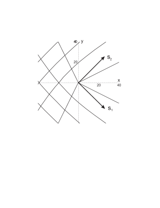
Figure 4: The wave pattern forming by two orthogonally directed flows with the velocities $s_{1}=s_{2}=0.9$. The directions of the velocities are shown by the arrows.

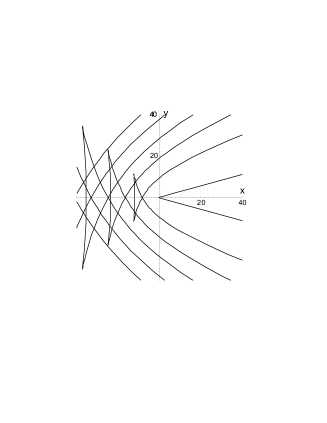
Figure 5: The wave pattern at $s_{1}=s_{2}=1$ and $\theta=0.45\pi$

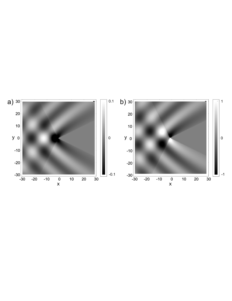
Figure 7: The total density (a) and the relative density (b) patterns (in relative units) for the stationary waves at $\theta=\pi/2$ and $s_{1}=s_{2}=0.9$.

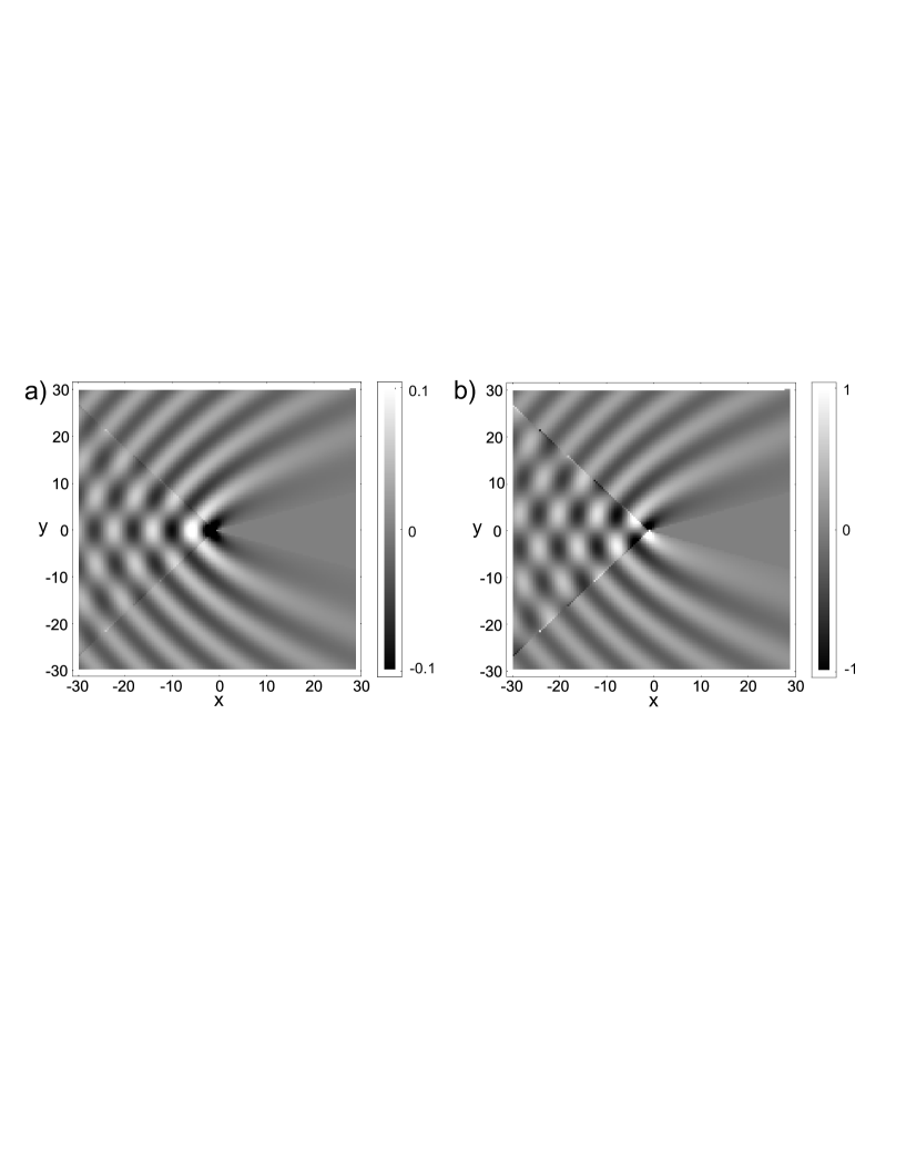
Figure 8: The same as in Fig. 7 at $\theta=0.45\pi$ and $s_{1}=s_{2}=1$.

References

- (1) I.M. Khalatnikov Zh. Eksp. Teor. Fiz. 32, 653 (1957), [Sov. Phys. JETP 5, 542 (1957)]; Pisma v Zh. Eksp. Teor. Fiz. 17, 534 (1973), [JETP Lett. 17, 386 (1973)].
- (2) A.F. Andreev, E.P. Bashkin, Zh. Eksp. Teor. Fiz. 69, 319 (1975), [Sov. Phys. JETP 42, 164 (1975)].
- (3) D.V. Fil, S.I. Shevchenko, Fiz. Nizk. Temp. 30, 1028 (2004), [Low Temp. Phys. 30, 770 (2004)].
- (4) D.V. Fil, S.I. Shevchenko, Phys. Rev. A 72, 013616 (2005).
- (5) N. G. Berloff, e-print arXiv:cond-mat/0412743.
- (6) H. Susanto, P. G. Kevrekidis, R. Carretero-Gonzalez, B. A. Malomed, D. J. Frantzeskakis, and A. R. Bishop, Phys. Rev. A 75, 055601 (2007).
- (7) V.I.Yukalov, E.P.Yukalova Laser Phys. Lett. 1, No.1, 50 (2004).
- (8) L.Yu. Kravchenko, D.V. Fil Fiz. Nizk. Temp. 33, 1347 (2007), [Low Temp. Phys. 33, 1023 (2007)].
-
(9)
D.S. Hall, M.R. Matthews, J.R. Ensher, C.E. Wieman,
E.A. Cornell, Phys. Rev. Lett. 81, 1539 (1998);
P Maddaloni, M. Modugno, C. Fort, F. Minardi, M. Inguscio, Phys. Rev. Lett. 85, 2413 (2000);
H.-J. Miesner, D. M. Stamper-Kurn, J. Stenger, S. Inouye, A. P. Chikkatur, and W. Ketterle, Phys. Rev. Lett. 82, 2228 (1999). - (10) K. M. Mertes, J. W. Merrill, R. Carretero-Gonzalez, D. J. Frantzeskakis, P. G. Kevrekidis, and D. S. Hall, Phys. Rev. Lett. 99, 190402 (2007).
-
(11)
G. Modugno, M. Modugno, F. Riboli, G. Roati, M.
Inguscio, Phys. Rev. Lett. 89, 190404 (2002);
M. Mudrich, S. Kraft, K. Singer, R. Grimm, A. Mosk, M. Weidenmüller, Phys. Rev. Lett. 88, 253001 (2002). - (12) G. Thalhammer, G. Barontini, L. De Sarlo, J. Catani, F. Minardi, and M. Inguscio, Phys. Rev. Lett. 100, 210402 (2008).
- (13) S. B. Papp, J. M. Pino, and C. E. Wieman, Phys. Rev. Lett. 101, 040402 (2008).
- (14) R.Onofrio, C.Raman, J.M.Vogels, J.Abo-Shaeer, A.P.Chikkatur and W.Ketterle Phys. Rev. Lett. 85, 2228 (2000).
- (15) G.B. Whitham, Linear and Nonlinear Waves, (Wiley- Interscience, New York, 1974).
- (16) Yu.G. Gladush, G.A. El, A. Gammal, and A.M. Kamchatnov Phys. Rev. A 75, 033619 (2007).
- (17) Yu. G. Gladush, A. M. Kamchatnov, Z. Shi, P. G. Kevrekidis, D. J. Frantzeskakis, and B. A. Malomed, e-print arXiv:0811.1891.
- (18) F. Dalfovo, S. Giorgini, L.P. Pitaevskii, S. Stringari, Rev. Mod. Phys. 71, 463 (1999).
- (19) N.N. Bogolyubov and N. N. Bogolyubov, Jr., Introduction to Quantum Statistical Mechanics, (World Scientific, Singapore, 1982).
- (20) W. Ketterle, D. S. Durfee, and D. M. Stamper-Kurn, in Bose-Einstein condensation in atomic gases, Proceedings of the International School of Physics Enrico Fermi, Course CXL, edited by M. Inguscio, S. Stringari, and C.E. Wieman (IOS Press, Amsterdam, 1999), pp. 67-176.
- (21) H. J. Lewandowski, D. M. Harber, D. L. Whitaker, and E. A. Cornell, Phys. Rev. Lett. 88, 070403 (2002).
- (22) H. Schmaljohann, M. Erhard, J. Kronjager, M. Kottke, S. van Staa, L. Cacciapuoti, J. J. Arlt, K. Bongs, and K. Sengstock, Phys. Rev. Lett. 92, 040402 (2004).
- (23) M.-S. Chang, C. D. Hamley, M. D. Barrett, J. A. Sauer, K. M. Fortier, W. Zhang, L. You, and M. S. Chapman, Phys. Rev. Lett. 92, 140403 (2004).
- (24) T. Kuwamoto, K. Araki, T. Eno, and T. Hirano, Phys. Rev. A 69, 063604 (2004).
- (25) J. M. Higbie, L. E. Sadler, S. Inouye, A. P. Chikkatur, S.R. Leslie, K. L. Moore, V. Savalli, and D. M. Stamper-Kurn, Phys. Rev. Lett. 95, 050401 (2005).
- (26) L. E. Sadler, J. M. Higbie, S. R. Leslie, M. Vengalattore, and D. M. Stamper-Kurn, Phys. Rev. Lett. 98, 110401 (2007).
- (27) L.Yu. Kravchenko, D.V. Fil, J. Phys.: Condens. Matter 20, 325235 (2008).
- (28) A. Amo, J. Lefrere, S. Pigeon, C. Adrados, C. Ciuti, I. Carusotto, R. Houdre, E. Giacobino, A. Bramati, e-print arXiv:0812.2748
- (29) M. Alpar, S. Langer, J. Sauls Astrophys. J. 282, 533 (1984).