HD-THEP-08-27
Fixing D7 Brane Positions
by F-Theory Fluxes
Abstract
To do realistic model building in type IIB supergravity, it is important to understand how to fix D7-brane positions by the choice of fluxes. More generally, F-theory model building requires the understanding of how fluxes determine the singularity structure (and hence gauge group and matter content) of the compactification. We analyse this problem in the simple setting of M-theory on . Given a certain flux which is consistent with the F-theory limit, we can explicitly derive the positions at which D7 branes or stacks of D7 branes are stabilised. The analysis is based on a parameterization of the moduli space of type IIB string theory on (including D7-brane positions) in terms of the periods of integral cycles of M-theory on . This allows us, in particular, to select a specific desired gauge group by the choice of flux numbers.
1 Introduction
Over the past years, significant progress in some of the central phenomenological problems of string theory compactifications has been made. These problems include, in particular, moduli stabilisation, SUSY breaking, inflation and the possibility of fine-tuning the cosmological constant in the landscape of flux vacua. Much of this has been realised most successfully and explicitly in type IIB Calabi–Yau orientifold models in the supergravity regime (for reviews, see e.g. [1, 2, 3, 4, 5]). However, obtaining the standard model particle spectrum remains difficult in this context, although successful local constructions exist[6, 7, 8, 9, 10, 11].
Motivated by the desire to make progress towards a type IIB (or, more generally, F-theory) derivation of the standard model, the present paper analyses the way in which fluxes determine D7 brane positions. This is central to weakly coupled type IIB models, where D7 brane stacks and their intersections are responsible for non-Abelian gauge symmetries and charged matter. We approach such compactifications from the F-theory perspective [12, 13], where the value of the type IIB dilaton is encoded in the complex structure of a torus attached to every point of the type IIB manifold. D7 branes are characterised by the degeneration loci of this torus fibration and non-Abelian gauge symmetries arise if the degeneration is so bad that the 8d compact space develops a singularity. Such singularities are associated with the shrinking of M-theory cycles, which is easy to ensure by the flux choice. In addition, in weakly coupled situations, the periods of M-theory cycles measure the relative positions of D7 branes.
Working in the simple setting of F-theory on (which corresponds to type IIB on ), we are able to demonstrate how fluxes stabilise D7 branes or stacks of D7 branes in a completely explicit fashion. This allows us to select a specific desired gauge group by the choice of flux numbers. As explained above, this is the same procedure required for the flux stabilisation of non-Abelian gauge symmetries in the (non-perturbative) F-theory context, which has recently attracted significant attention in the context of GUT model building [6, 7, 14, 15, 16]. We therefore expect that straightforward generalisations of our methods will be useful both for more complicated D7 brane models as well as for their non-perturbative F-theory cousins.
Moduli stabilisation by fluxes in M-theory on has been studied extensively in the past, especially in relation with the type IIB dual (see, e.g. [17, 18, 19]). In our work we derive the flux potential for the geometric moduli from dimensional reduction. We express it in a form manifestly invariant under the symmetry of the moduli space. In this form, it is immediate to see how the minimisation condition is translated into a condition on fluxes and on geometric data of the two ’s. We find all Minkowski minima, both supersymmetric and non-supersymmetric. An analogous explicit search for (supersymmetric) flux vacua has been reported in [20]. Our results are more general since we do not restrict ourselves to attractive surfaces, where a maximal number of integral 2-cycles are holomorphic.111At a technical level, this means that only a discrete set of values are allowed for the various complex structure moduli. There is then also only a very restricted set of fluxes which are suitable for stabilising such points.
Our analysis of moduli stabilisation is also more explicit than the previous works on , since we use a parameterisation of D7-brane motion by the size of integral two-cycles, as derived in [21]. Thus, at least in the weak coupling limit, we have a simple geometric interpretation for every integral basis cycle. Using the choice of flux numbers, this gives us full control over the positions of 4 O7 planes and 16 D7 branes moving on a base (corresponding to type IIB on ).
Our techniques can be used to study the stabilisation of all the gauge groups that can be realised by F-theory on . It turns out that tadpole cancellation is very restrictive and allows only very special flux choices.
We begin our analysis in Section 2 with a derivation of the flux potential, which closely follows the generic Calabi-Yau derivation of [23, 22, 24]. We emphasise the fact that, due to the hyper-Kähler structure of , its geometric moduli space can be visualised by the motion of a three-plane in the 22-dimensional space of homology classes of two-cycles. This three-plane is spanned by the real and imaginary parts of the holomorphic 2-form and by the Kähler form. The resulting symmetry of the geometric moduli is manifest in the expression for the scalar potential we arrive at. The three-dimensional theory also has a number of gauge fields, and the flux induces mass terms for some of them, which we derive explicitly. This breaking of gauge symmetries can be understood in the dual type IIB picture as the gauging of some shift symmetry in the flux background.
In Section 3 we analyse the minima of the above flux potential. To preserve four-dimensional Poincaré invariance, we consider 4-form fluxes that belong to . A flux of this form gives rise to a linear map between the spaces of two-cycles of the two ’s: integrating the flux on a 2-cycle of one we get a 2-form on the other (which is Poincaré dual to a 2-cycle). Minkowski vacua arise if the flux maps the three-planes determining the metric of the ’s onto each other. We derive the conditions the flux matrix has to satisfy in order for two such planes to exist and to be completely fixed by the choice of fluxes. Furthermore, we clarify the more restrictive conditions under which the plane determined by the flux is consistent with the F-theory limit. In this case, the plane cannot be fixed completely. The unfixed moduli correspond to Wilson lines around the of the type IIB model which decompactifies in the F-theory limit. These degrees of freedom are not part of the moduli space of type IIB compactified to four dimensions, as they characterise the (unphysical) constant background value of one component of the four-dimensional vector fields. In fact, the corresponding propagating degrees of freedom become part of the four-dimensional vector fields (see [25] for a comprehensive analysis of the duality map between the 4d fields of M-theory on and type IIB string theory on ).
The main point of our paper, the explicit stabilisation of D-brane positions, is the subject of Section 4. After recalling the parameterisation of D7-brane motion in terms of M-theory cycles derived in [21], we provide explicit examples of flux matrices which fix situations with gauge symmetries , and . In all cases we also fix the complex structure moduli of the lower . The first case corresponds to the orientifold, where 4 D7 branes lie on top of each O7 plane. In the second case, one D7 brane is moved away from an O plane. Finally, in the third case, a stack of two D7 branes is separated from one of the O planes. In these examples almost all the Kähler moduli (which correspond to deformations of the lower and do not affect the positions of the D7 branes) are not stabilised. When one of them is stabilised, a Kähler modulus of the upper is stabilised, too. As mentioned before, this corresponds to some gauge field becoming massive. To clarify this point, we present two examples where one of the D7 branes is fixed at a certain distance from its O plane: In the first example, one further Kähler modulus is fixed, breaking the gauge group. This phenomenon of gauging by fluxes is common in flux compactifications[26, 27, 28, 29]. In the second example, we stabilise the single D7 brane without fixing further Kähler moduli and hence without gauge symmetry breaking. We also provide an example where almost all moduli are fixed. In this case, only the fibre volume of F-theory, the volume moduli of the two s, and three metric moduli of the lower remain undetermined.
Section 5 contains a brief discussion of supersymmetry. Generically, we obtain vacua of no-scale type. For specific, non-generic choices of the flux matrix, we find three-dimensional or supersymmetry. To determine the amount of surviving supersymmetry, it suffices to know the eigenvalues of the flux matrix restricted to the two three-planes.
After summarizing our main results in Section 6, we collect some technical issues in the appendices. Appendix A contains some basic definitions concerning the geometry of , Appendix B gives the flux potential in terms of the two superpotentials of M-theory compactifications. Some facts about self-adjoint operators on spaces with indefinite metric are collected in Appendix C. Finally, Appendix D supplies some further details concerning the F-theory limit, especially the way in which certain M-theory moduli are lost in the F-theory limit.
2 Flux Potential
In this chapter we compactify M-theory to three dimensions on and analyse the effects of four-form flux. The main new points of our presentation are the following: We maintain a manifest symmetry of the moduli space of in the calculation of the potential in Section 2.2. Furthermore, we explicitly derive the flux-induced masses for the vector fields arising from the three-form in Section 2.3.
2.1 M-Theory on
The compactification of M-theory on a generic four-fold is described in detail in[22]. Here we specialise to the case of . To distinguish the two ’s, we write the compactification manifold as . Correspondingly, all quantities related to the second will have a tilde.
The relevant M-theory bosonic action is[30]
| (2.1) | ||||
where is the eleven-dimensional Planck length, , and and are polynomials of degree 4 in the curvature tensor [31, 32]. When we compactify on , we obtain a three-dimensional theory with eight supercharges, i.e. in three dimensions. This can be inferred from the fact that each has holonomy group and correspondingly two invariant spinors.
Let us analyse the geometric moduli. is a hyper-Kähler manifold: its metric is defined by three two-forms in plus the overall scale. is a 22-dimensional vector space equipped with a natural scalar product,222 Throughout this work, we freely identify forms, their cohomology classes, the Poincaré-dual cycles and their homology classes.
| (2.2) |
which has signature , i.e. there are three positive-norm directions. The three vectors defining the metric must have positive norm and be orthogonal to each other. Hence they can be normalised according to . The Kähler form and holomorphic two-form and can then be given as
| (2.3) |
This definition is not unique: we have an of possible complex structures and associated Kähler forms. Each of them defines the same metric, which is then invariant under the that rotates the ’s.
The motion in moduli space can now be visualised as the motion of the three-plane spanned by the ’s, which is characterised by the deformations of the preserving orthonormality. The corresponding are in the subspace orthogonal to , which is 19-dimensional. Together with the volume, this gives scalars in the moduli space of one . The same parameterisation can be used for the second , where the corresponding scalars are and the components of . Altogether one finds scalars from the metric on . Furthermore, since has no harmonic one-forms, there are no 3d vectors coming from the metric.
2.2 The Scalar Potential
We now allow for an expectation value for the field strength of the form
| (2.4) |
where (with ) is an integral basis of . The flux satisfies a (Dirac) quantisation condition333 The precise quantisation condition for a generic fourfold is , where is the first Pontryagin class[33]. Since is even for , the quantisation condition becomes simply . : . In the following, we will always denote this type of flux by while the generic four-form field strength will be .
The flux potential for the moduli is found by reducing the M-theory action. In the presence of fluxes, the solution to the equations of motion is a warped product of a Calabi–Yau fourfold and a three-dimensional non-compact space[22, 19, 34]. In the following, we neglect backreaction and work with the undeformed Calabi–Yau space as the internal manifold. The underlying assumption is that, in analogy to[34], for any zero-energy minimum of the unwarped potential a corresponding zero-energy warped solution will always exist. After Weyl rescaling, the potential is given by[24]
| (2.5) |
where is the Euler number of the compact manifold. For , it is . Given our previous discussion of moduli space, we expect that (2.5) will be invariant under rotations once we express the metric in terms of and .
In the absence of spacetime-filling branes, the cancellation of -brane-charge on the compact manifold requires[22]
| (2.6) |
This allows us to express the second term in (2.5) through the flux. It is convenient to set and to introduce a volume-independent potential by writing . Here is the volume of . Our result now reads
| (2.7) |
with given by (2.4).
On , each can be split into a sum of two vectors, parallel and perpendicular to the 3-plane :
| (2.8) |
Here is the projector on the subspace orthogonal to . The first term, which corresponds to the projection on , has been given in a more explicit form using the orthonormal basis of the plane for later convenience. The two terms of (2.8) represent a selfdual and an anti-selfdual two-form[23], allowing us to write the Hodge dual of a basis vector as
| (2.9) |
The same applies to .
If we insert (2.4) and (2.8) into the expression (2.7) for and we use the relation (2.9) for the action of the Hodge , we find
| (2.10) | ||||
Since
| (2.11) |
we can write as
| (2.12) | ||||
To write it in a more compact form, we define two natural homomorphisms and by
| (2.13) |
where , and , represent the metrics in the bases , . The operator is the adjoint of , i.e. . The matrix components of these operators are and .
The moduli potential is then given by
| (2.14) |
As expected, it is symmetric under rotation of the ’s and of the ’s444 The projectors and are obviously symmetric as they project onto the space orthogonal to all the ’s..
This potential is positive definite since the metrics for and defined in (2.2) are negative definite on the subspace orthogonal to the ’s and the ’s. We note also that the volumes of the two ’s are flat directions parameterizing the degeneracy of the absolute minimum of the potential, in which .
We can also rewrite this potential expressing the projectors through the ’s:
| (2.15) |
This is again manifestly symmetric under rotations. The potential can also be expressed in terms of two superpotentials (see Appendix B). We will not need this formulation in the following.
In (2.4) we have only considered fluxes with two legs on each . More generally the flux could be of this form:
| (2.16) |
where and are the volume forms on and .555 The normalisation is . To obtain the general potential, we need to compute . Using our previous result for and the Hodge duals
| (2.17) |
of and , we find
| (2.18) | ||||
With the substitutions and , the potential can be concisely written as
| (2.19) |
This potential is still positive definite and has minima at points where it vanishes, but it now has only one unavoidable flat direction, the overall volume of . The ratio of the volumes is fixed at .
2.3 Gauge Symmetry Breaking by Flux
In our context, F-theory emerges from the duality between M-theory on , with being elliptically fibred, and type IIB on . The F-theory limit consists in taking the fibre volume to zero on the M-theory side, and in taking the radius of the to infinity on the type IIB side (see Section 3.2 for the details of this limit). Before analysing the effect of gauge symmetry breaking by fluxes, we recall the different origins of four-dimensional gauge fields in type IIB and in F-theory.
Type IIB theory on contains 16 vectors from gauge theories living on D7 branes and 4 vectors from the reduction of and along one-cycles of . In three dimensions, one then has 20 three-dimensional gauge fields and 20 scalars corresponding to Wilson lines along the . In the F-theory limit, these scalars combine with the vectors to give the required 20 four-dimensional vector fields.
In M-theory on , vectors arise from the reduction of the three-form along two-cycles in or . Since we are in three dimensions we have the freedom to dualise some of these vectors, treating them as three-dimensional scalars. To match the type IIB description, the correct choice is to treat only the fields coming from the reduction of on two-cycles of as vectors666A simple intuitive argument for this choice can be given by comparing the seven-dimensional theories coming from M-theory on and type IIB on . In M-theory, we have seven-dimensional vectors associated with two-cycles stretched between the pairs of degeneration loci of the fibre (which characterise D7 branes). In type IIB, the corresponding vectors come directly from the D7-brane world-volume theories. The fact that they are associated with branes rather than with pairs of branes is simply a matter of basis choice in the space of s.. This reduction gives 22 vectors in three dimensions. However, since is elliptically fibred, there are two distinguished two-cycles: the base and the fibre. They require a special treatment in the F-theory limit and, as a result, three-dimensional vectors arising from these two cycles do not become four-dimensional gauge fields in the F-theory limit. Instead, one of them corresponds to the type IIB metric with one leg on the , while the other is related to with three legs on [25]. We will not consider these two vectors in the following and focus on the remaining 20 three-dimensional vectors associated with the reduction of on generic two-cycles of .
Each of these vectors absorbs a three-dimensional scalar (corresponding to a Wilson line degree of freedom on the type IIB side) to become a four-dimensional vector. These 20 scalars come from the metric moduli space of . More precisely, 18 arise from the variations of the Kähler form in directions orthogonal to the three-plane and to the base-fibre subspace777 For an elliptically fibred , two directions of the three-plane are orthogonal to base and fibre subspace, while has a component along the base-fibre subspace. This explains the above number of independent variations as . The variation of within the base-fibre subspace corresponds to part of the metric in the F-theory limit. . The two remaining scalars come from variations and of the holomorphic two-form which lie in the base-fibre subspace and are orthogonal to . For a detailed analysis of the matching of fields on both sides of the duality, see [25].
Given these preliminaries, it is now intuitively clear why F-theory flux generically breaks gauge symmetries: The flux induces a potential for the metric moduli, making them massive. This applies, in particular, to those moduli which become vector degrees of freedom in four dimensions. Hence, the full four-dimensional vector becomes massive by Lorentz invariance888 Correspondingly in type IIB, putting two-form flux on certain cycles of wrapped D7 branes breaks the gauge symmetry of the brane[28, 26, 27, 29]..
To derive the vector mass term explicitly, we begin by writing in the form
| (2.20) |
Here and are basis two-forms on the factors, and are one-form fields in three dimensions, and is the contribution responsible for the four-form flux (which is only locally defined). As before, the flux is given by .
In the reduction of the action, the term leads to the flux term (which is irrelevant for our present discussion) and to kinetic terms for and . The metric for the kinetic terms is given by
| (2.21) | |||
| (2.22) |
We have split off the volume dependence, so that and are dimensionless. Note that these metrics are positive definite since the subspace orthogonal to the three-plane has negative-definite metric. Note also that there is no kinetic mixing between the and the since .
We now turn to the Chern–Simons term . Evaluating this term with of the form (2.20), we see that the contribution vanishes: has three legs on , so would need to have three legs on and five legs on . This is, however, inconsistent with (2.20). The other contributions give
| (2.23) |
Thus, the flux matrix couples and . (Note that flux proportional to the volume forms of and would, in addition, lead to couplings and .)
We have now arrived at the three-dimensional effective action
| (2.24) | ||||
As explained before, only the vectors become four-dimensional vectors in the F-theory limit[25]. It is convenient to dualise the remaining vectors , replacing them by scalars . To this end, we turn the equation of motion,
| (2.25) |
into a Bianchi identity by defining through
| (2.26) |
It follows that the have to transform non-trivially under the gauge transformations of the :
| (2.27) |
In other words, the vectors gauge shift symmetries of the scalars , with the charges determined by the flux.
The equation of motion of follows formally from , the Bianchi identity of . Since on , we find
| (2.28) |
We now want to find a gauge invariant action from which this equation of motion can be derived. Such an action is given by
| (2.29) |
The corresponding Einstein-Hilbert term has the usual volume prefactor and can be brought to canonical form by a Weyl rescaling of the three-dimensional metric. This gives the kinetic term of the vectors a prefactor , which we can absorb in a redefinition of . The resulting mass matrix has the form
| (2.30) |
which is positive semidefinite since is a positive definite metric. The number of gauge fields which become massive is determined by the rank of the flux matrix. Comparing with Eq. (2.14), we see that the masses are of the same order as the masses of the flux stabilised geometric moduli. This confirms the intuitive idea put forward at the beginning of this section: The vectors and some geometric moduli are combined in the F-theory limit to produce four-dimensional vectors. For this to work in the presence of fluxes, both the three-dimensional vectors and scalars need to have the same flux-induced masses.
3 Moduli Stabilisation
In this section we turn to the flux stabilisation of moduli. First, we will analyse under which conditions the potential (2.14) has minima at , and whether there are flat directions. Then we will see which restrictions we have to impose in order to map the M-theory situation to F-theory, and discuss possible implications for gauge symmetry breaking.
Let us first comment on the flux components which are proportional to the volume forms. In what follows, we do not consider these components, in other words, we set . The reason is that we want to end up with a Lorentz-invariant four-dimensional theory. By going through the M-theory/F-theory duality explicitly, one can see that this requires that the flux needs to have exactly one leg in the fibre torus and hence two legs along each . Thus, we can without loss of generality use a flux in the form of Eq. (2.4), and the associated potential (2.14).
3.1 Minkowski Minima
Clearly, the potential (2.14) cannot stabilise the volumes and . They are runaway directions in general, and flat directions exactly if the term in brackets vanishes. This term is a sum of positive definite terms, so each of these must vanish if we want to realise a minimum with vanishing energy. Since each term contains a projection onto the subspace orthogonal to the three-planes spanned by the ’s and ’s, the bracket clearly vanishes if and only if the flux homomorphisms map the three-planes into each other, though not necessarily bijectively:
| (3.1) |
Note that what is required is not merely the existence of three-dimensional subspaces which are mapped to each other, but that both subspaces are positive-norm. If the metrics were positive definite, this condition would be trivial since any real matrix can be diagonalised by choosing appropriate bases in and .
We will now show that the conditions (3.1) are equivalent to the conditions that the map is diagonalisable and all its eigenvalues are real and non-negative999Note that maps onto itself, so it makes sense to speak of eigenvalues and eigenvectors. Note also, however, that although is a selfadjoint operator, this does not imply that its eigenvalues are real since the metric is indefinite. We have collected some facts about linear algebra on spaces with indefinite metric in Appendix C..
Let us assume that there exist two three-planes and such that the relations (3.1) hold. The cohomology groups can be decomposed into orthogonal subspaces, and , such that the metric (2.2) defined by the wedge product is positive (negative) definite on and ( and ). The conditions (3.1) imply that and are block-diagonal, i.e. we also have and . It is then obvious that the selfadjoint operator obeys101010Similarly obeys .
| (3.2) |
As each block is selfadjoint relative to definite metrics, is diagonalisable with real and non-negative eigenvalues.
We now show that the converse also holds. Assume that is diagonalisable with non-negative eigenvalues111111In this case, because of the non-degeneracy of the inner product, there alway exists a basis of non-null eigenvectors.. This defines a decomposition of in , where is the three-dimensional subspace given by the eigenvectors with positive norm. The fact that maps into itself implies that maps positive norm vectors into positive norm vectors: Indeed, give ,
| (3.3) |
If is invertible (non-zero eigenvalues in ), then we can define as the image of . The fact that is invariant under implies that the image of is and (3.1) is proved. The case in which has non-trivial kernel does not present any complication. Since the kernel of coincides with the kernel of 121212Since and are adjoint to each other, there is an orthogonal decomposition . Take ; since is both in and in , it is the zero vector, proving that ., the image of is no more three dimensional. One then defines as the image of plus the positive norm vectors in the kernel of .
To summarise, the conditions (3.1) are equivalent to the condition that is diagonalisable and all its eigenvalues are real and non-negative. In this case (see Appendix C) the matrices for , and take the form
| (3.4) |
in appropriate bases, where are the eigenvalues of relative to positive norm eigenvectors, while are relative to negative norm eigenvectors.
Finally, we want to see whether there are flat directions. The potential has a flat direction, if there are infinitesimally different positions of the three-planes which give Minkowski minima. Given a flux (such that is diagonalizable with positive eigenvalues), the minima correspond to () generated by the positive norm eigenvectors of (). If all the eigenvalues are different from each other, there can be only three positive norm eigenvectors, and the minimum is isolated. If a positive norm and a negative norm eigenvector have the same eigenvalue, e.g. , then a flat direction arises: Any three-dimensional space spanned by , and () will give a different that still satisfies the conditions (3.1). It is easy to see that an analogous flat direction develops for . Note that if some are degenerate then the rotation of the vectors does not move the three-planes.
This shows that flat directions of the potential are absent if and only if the sets of eigenvalues and are pairwise distinct.
3.2 F-Theory Limit
We are interested in stabilising points in the moduli space of which can be mapped to F-theory. This means we require that is an elliptic fibration over a base , and that the fibre volume vanishes.
The first requirement means that needs to have two elements (the base) and (the fibre) in the Picard group, i.e. two integral (1,1)-cycles, whose intersection matrix is
| (3.5) |
Note that by a change of basis from to , this intersection matrix is equivalent to one block in the general form (A.1) of the metric in an integral basis.
As (1,1)-cycles, and must be orthogonal to the holomorphic two-form. In our case this means that the plane has a two-dimensional subspace orthogonal orthogonal to . This subspace is spanned by the real and imaginary part of the holomorphic two-form . On the other hand, contains the third positive-norm direction, so cannot be also orthogonal to . For the following discussion it is convenient to consider directly the Kähler form instead of and separately. The Kähler form can be parametrised as
| (3.6) |
where is an orthonormal basis (i.e. ) of the space orthogonal to , and . This is the most general form of for an elliptically fibred .
Now we turn to the second requirement: the fibre must have vanishing volume. This is what is called the F-theory limit. For the Kähler form (3.6), we find the volumes of the fibre and the base to be131313 More generally the volume of a two-cycle is given by the projection on the three-plane , multiplied by the volume:
| (3.7) |
Hence, the F-theory limit involves , and in this limit, the base volume will be given by . On the other hand, the volume of the entire is
| (3.8) |
This volume is required to be positive, so we get a bound on the ,
| (3.9) |
Thus, in the F-theory limit we have to take the to zero at least as fast as . Once the limit is taken, the volume of vanishes and the Kähler form is given by
| (3.10) |
regardless of the initial value of the . Note that the constraint (3.9) is consistent with the intuitive picture of the fibre torus shrinking simultaneously in both directions: The measure the volume of cycles which have one leg in the fibre and one in the base, so they shrink like the square root of the fibre volume .
The Kähler moduli space is reduced in the F-theory limit: We lose not only the direction along which we take the limit, but also all transverse directions except for the base volume , which becomes the single Kähler modulus of the torus orbifold. In the duality to type IIB on , the parametrise Wilson lines of the gauge fields along the as long as the fibre volume is finite. In the F-theory limit, which corresponds to the radius of the going to infinity, the Wilson lines disappear from the moduli space. The propapagating degrees of freedom related to them combine with the three-dimensional vectors from the three-form reduced along two-cycles of to form four-dimensional vectors (cf. Section 2.3, see also [25]).
From this perspective, we see that it is important not to fix the modulus controlling the size of the fibre. In fact, if we leave it unfixed, we have a line in the M-theory moduli space corresponding to this flat direction of the potential. Of this line, only the point at infinity () corresponds to F-theory. This limit is singular in the sense that the F-theory point is not strictly speaking in the moduli space of , but on its boundary. As we show in Appendix D, this point is at infinite distance from every other point in the moduli space of , and it actually corresponds to the decompactification limit in type IIB.
To see which fluxes are compatible with this limit, we first note that there must be no flux along either or because Lorentz invariance of the four-dimensional theory requires that the flux must have exactly one leg along the fibre. This means that in a basis of consisting of , and orthogonal forms, the flux matrix must be of the form
| (3.11) |
This leads to a with two rows and columns of zeroes,
| (3.12) |
hence the direction along which we take the F-theory limit is automatically flat.
To discuss the matrix form of , it is convenient to choose an equivalent basis for , i.e. a basis containing and and 20 orthogonal vectors. We then restrict to fluxes of the type
| (3.13) |
although this is not the most general form. Here, is a matrix which we will also call for simplicity.
4 Brane Localisation
One of our aims is to find a flux that fixes a given configuration of branes. The results obtained so far allow us to do that: As we will review in the next subsection, the positions of the D7 branes are encoded in the complex structure of [21]. This can be understood as follows: We can find certain cycles which measure the distance between branes. A given brane configuration can thus be characterised by the volumes of such cycles. Most relevant for the low-energy theory is the question whether there are brane stacks (corresponding to gauge enhancement) which is signalled by the vanishing of interbrane cycles. So choosing a given brane configuration determines a set of integral cycles which are to shrink, i.e. which should be orthogonal to the complex structure141414These are cycles with one leg in the base and one in the fibre and which are orthogonal to once we take the F-theory limit (3.10).. We want to find what is the flux that fixes such a complex structure.
The flux needs to satisfy some constraints: It must be integral and it must satisfy the tadpole cancellation condition (2.6). The first condition means that the entries of the flux matrix in a basis of integral cycles must be integers. The tadpole cancellation condition translates into a condition on the trace of ,
| (4.1) |
Of course, we also require that the flux gives Minkowski minima, i.e. needs to have only non-negative eigenvalues. These conditions turn out to be rather restrictive, and a scan of all -matrices is computationally beyond our reach. Fortunately, the block-diagonal structure alluded to above allows us to restrict to smaller submatrices of size or , where an exhaustive scan is feasible.
4.1 D-Brane Positions and Complex Structure
In the weak coupling limit, in which the F-theory background can be described by perturbative type IIB theory, the complex structure deformations of the upper have an interpretation in terms of the movement of D-branes and O-planes on [13]. From the perspective of the elliptically fibred , D-branes and O-planes are points on the base where the fibre degenerates. The positions of these points are encoded in the complex structure of : The 18 complex structure deformations151515 These are the deformations of and in the space orthogonal to and . specify the 16 D-brane positions, the complex structure of , and the value of the complex dilaton. The map between the two descriptions is worked out in detail in [21]. In the following, we summarise the basic results.
When several D-branes coincide, the surface develops singularities which reflect the corresponding gauge enhancement [35, 36, 37, 38, 39, 40]. These singularities can also be seen to arise when the volume of certain cycles shrinks to zero:
| (4.2) |
Note that these cycles have one leg on the base and and one leg on the fibre torus, so 161616Since we are interested in the F-theory limit, we will only consider vacua corresponding to being in the block .. Hence their volume is given by . If the are integral cycles (for the structure of integral cycles on see Appendix A) with self-intersection , their shrinking produces a singularity that corresponds to a gauge enhancement. Since these cycles can be thought of as measuring distances between branes, this is equivalent to D-branes that are coinciding. The Cartan matrix that displays the gauge enhancement is given by the intersection matrix of the shrinking .
Let us consider an point at which degenerates to . From the D-brane perspective this corresponds to putting four D-branes on each of the four O-planes. In terms of the basis given in Appendix A, the complex structure of is given by
| (4.3) |
For the sake of brevity we have introduced171717Note that although , , , and are forms on , we omit the tildes to avoid unnecessary notational clutter.
| (4.4) |
where
| (4.5) |
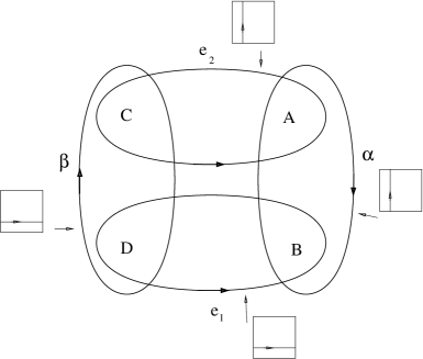
describe the mixing of cycles from the and blocks. Note that they can be interpreted as Wilson lines, breaking to in the duality to heterotic string theory. The cycles that are dual to the forms and are shown in Figure 1.
The parameter describes the positions of the four O-planes, which is equivalent to the complex structure of the in type IIB before orientifolding. The dilaton, which is constant in this configuration, is given by the complex structure of the fibre torus, .
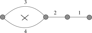
One can check that the cycles which have vanishing periods at an point span the lattice . They are given by
| 1 2 3 4 . | (4.11) |
These cycles can be constructed geometrically. Their projections to the base connect the D-branes and are displayed for one block in Figure 2.
We can now move away from the configuration by rotating . A convenient parameterisation is given by
| (4.12) |
with shifted block vectors . Explicitly, they are
| (4.13) |
The are orthogonal to and and still satisfy . Using Table (4.11) and Figure 2, one can show [21] that the are the positions of the branes relative to their respective O-planes in the double cover of .
Now we can deduce the brane positions and the gauge enhancement from a given expansion of the holomorphic two-form (which is equivalent to knowing the complex structure of ). We can either match any expansion of in the basis given in Appendix A to (4.12), or we can compute the intersection numbers between and the cycles given in Table 4.11 to find the periods of the cycles of . In this way we obtain the value of the dilaton and the D-brane and O-plane positions. Note that contrary to the basis given by and the cycles in Table (4.11), the basis we used in the expansion (4.12) is not an integral basis (as the are half-integral).
4.2 Fixing D7-brane Configurations by Fluxes
We are now ready to outline a systematic procedure for choosing a flux which fixes a given D7-brane gauge group. In particular, we will be interested in non-Abelian gauge enhancement. The Cartan matrix of the underlying Lie-Algebra is given by the intersection matrix of the lattice of shrinking two-cycles. Thus, we need to understand which fluxes make a particular subspace of two-cycles shrink. We will take these cycles as part of the basis orthogonal to discussed at the end of Section 3. Then we consider the orthogonal lattice, i.e. the lattice made up of (integral) cycles orthogonal to the shrinking ones (and to ). Choosing an integral basis for this lattice completes the basis of cycles of orthogonal to . Note that in this basis the metric on is block-diagonal, with a negative definite block for the subspace of shrinking cycles. We also choose a basis of integral cycles of such that the metric has two blocks with the same dimensions as on the side.
In this basis it is easy to write down a flux that fixes orthogonal to the shrinking cycles: It can be taken to have the block-diagonal form181818Actually, it is enough that is of this form.
| (4.14) |
Thus, when diagonalising , the positive norm eigenvectors are in the first block and hence orthogonal to the shrinking cycles.
One has finally to check whether there are more shrinking cycles than those we imposed.
4.3 Fixing an Point
In this section, we will follow the procedure described in the previous section to construct a flux that fixes the F-theory moduli corresponding to four D7 branes on top of each O7 plane. This configuration is realised when there are sixteen shrinking cycles whose intersection matrix is . These shrinking cycles are given by the four blocks as defined in (4.11). The basis of the orthogonal lattice is given by (see Eq. (4.4)). Since the only nonvanishing intersections in this set are , the intersection matrix is
| (4.15) |
For we choose the same basis. Note that we are ignoring the block spanned by base and fibre.
Then we take the flux matrix with respect to these bases to be
| (4.19) |
where and are blocks (which form the of (4.14)) and the zero block is ( of (4.14)). If and satisfy the condition to have minima, then one is fixed along the space , while the other is fixed in the space . This immediately gives a complex structure that is orthogonal to the blocks and hence realises an point.
An explicit example of an integral flux that satisfies the tadpole cancellation condition (tr) and fixes an point is given by:
| (4.24) |
The corresponding blocks for are
| (4.29) |
and the corresponding eigenvalues are
| (4.30) |
We see that their sum is precisely , as required by tadpole cancellation, and that they are all non-negative, as required by the minimum condition. Moreover, the ones corresponding to positive norm eigenvectors are different from those relative to negative norm eigenvectors, as required by the stabilisation condition.
The positive norm eigenvectors of the two matrices give , :
| (4.31) |
From the comparison of with the general form (4.12), we see that indeed the complex structure is fixed at a (non-integral) point where , and that the complex structures of base and fibre are given by
| (4.32) |
Since is the type IIB axiodilaton, we have stabilised the string coupling at a moderately small value of However, we can probably realise smaller coupling by considering generic matrices rather than the block structure of Eq. (4.19).
This flux fixes also the deformations of and . On the other hand, and are eigenvectors of and relative to zero eigenvalues. Then their deformation along all negative eigenvectors relative to zero eigenvalues are left unfixed. In type IIB, this corresponds to leaving unfixed Kähler moduli of , while fixing the complex structure and the D7-brane positions. The unfixed deformations of correspond to gauge fields in type IIB that remain massless [25]. In the studied case, two of the deformations of and , the ones along , are fixed (as is different from zero). Fixing a deformation of corresponds to giving a mass to the corresponding gauge field in type IIB dual. In fact, this flux corresponds to the type IIB flux that makes one four-dimensional vector massive [26, 27, 28, 29]. One can see this also from the M-theory point of view: One three-dimensional vector gets a mass from fluxes. This vector combines with the deformation of to give a four-dimensional massive vector.
Finally we note that the lower is generically non-singular, as will generically not be orthogonal to the block cycles.
As a second example we will reproduce one of the solutions given in [20] by using our methods. As it is discussed there, attractive surfaces are classified in terms of a matrix
| (4.33) |
in which and are integral two-forms. The holomorphic two-form of is then given by
| (4.34) |
Of the 13 pairs of attractive ’s given in [20], we will discuss the one defined by
| (4.35) |
This pair has the advantage that both ’s have an orientifold interpretation which means that we can expand and in terms of , , and (and similarly, for the lower , and in terms of , , and ). Clearly, there are many ways to do this which correspond to different embeddings of the lattice spanned by and into the lattice spanned by , , and . We make the following choice:
| (4.36) |
According to [20], stabilization at this point occurs through the flux
| (4.37) |
with . In the basis given by and , the flux matrix reads
| (4.38) |
The positive norm eigenvectors of are given by and . Rescaling the second one so that they both have the same norm, we arrive at . This is precisely the same result as what one obtains from inserting (4.36) into (4.34).
The eigenvalues of are , . In the last section we will see that this corresponds to an (4d) vacuum. Moreover, in this case all the Kähler moduli of both ’s are left unfixed by fluxes, as all the eigenvalues are equal to zero.
4.4 Moving Branes by Fluxes
Now we want to see how to change the flux (4.19), with and given by (4.24), to fix a different D7-brane configuration in which some D7 branes have been moved away from the orientifold planes. In particular, we will find fluxes that fix configurations where we move one or two branes off one of the stacks, breaking one to or . In the following we will consider only the -block. The cycles belonging to blocks will remain shrunk.
Moving one D7 brane from one stack in type IIB corresponds to blowing up one of the 4 cycles of this block. For the first example, consider the complex structure determined by (4.12) with and al other . One can check that all cycles given in Table 4.11 except remain orthogonal to . Looking at Figure 2, it is clear that this means we have moved one D-brane away from the O-plane, as claimed. Thus is broken to . At the same time the cycles that remain shrunk in block have an intersection matrix that is equivalent to minus the Cartan matrix of . This means that we have effectively crossed out the first line and the first column of the Cartan matrix of by removing from the set of shrunk cycles:
| (4.39) |
We want an integral basis in which shrunk and blown-up cycles do not intersect each other. To achieve this we keep the shrunk cycles , , and instead of we take the integral cycle (see (4.13)) to describe the brane motion in block . We find the intersection matrix
| (4.40) |
We choose an analogous basis for the lower .
The basis , is the one that gives the flux matrix the block-diagonal form (4.14), with the shrinking cycles given by and the orthogonal ones by . Such a block-diagonal flux matrix generally gives a component along . An example is given by:
| (4.41) |
where the block is with respect to the cycles for both ’s. From the type IIB perspective, we are also turning on fluxes on the D7 branes.
satisfies the tadpole cancellation condition. The eigenvalues corresponding to the first block are the same as in Eq. (4.30), the ones in the second block are
| (4.42) |
They are all positive and different from each other. The positive norm eigenvectors give and :
| (4.43) |
The corresponding is orthogonal the cycles with intersection matrix , but it is not orthogonal to the cycle which is now blown up, at a volume . This corresponds to the motion of one D7 brane away from the orientifold plane of block . Note that again the coupling is moderately weak, .
We also note that, with respect to our -example, we have fixed one more deformation of and one of . The stabilisation of the extra deformation is the signal of a mass for the gauge field on the D7 brane that has been moved. This mass is explained in type IIB by the fact that D7 fluxes gauge some shift symmetries by vectors on the branes. Since the on the brane is broken, the resulting gauge group is [26, 27, 28, 29].
In the example studied above, we have given a flux that fixes the desired brane configuration. Moreover it fixes one further deformation of and one of , with respect to the example presented before. This is related to the fact that the rank of the block has been increased to ; so we get two negative norm eigenvectors with non-zero eigenvalues. But we can choose a different flux, such that the number of negative norm eigenvectors relative to non-zero eigenvalues does not change with respect to the case:
| (4.44) |
where the block is still with respect to the cycles .
Again, satisfies the tadpole cancellation condition. The eigenvalues relative to the first block are the same as in Eq. (4.30). The eigenvalues of the second block are
| (4.45) |
They are all non-negative and different from each other. The positive norm eigenvectors give and :
| (4.46) |
As before, the corresponding is orthogonal the cycles with intersection matrix , but it is not orthogonal to the cycle which is now blown up, at a volume . Again, one D7 brane is moved from the orientifold plane of block .
In this case, we do not break any further . In fact, the flux we turned on contributes to the gauging of an isometry that has been gauged also in the case. This can be easily understood in the M-theory context, where the relevant gauge field is one of the .
As a further example, let us choose and all other . We now find that . For all other cycles in Table (4.11) the intersection with still vanishes, so we have blown up a different cycle than in the previous examples. From the assignment between cycles and forms it is clear that we have moved two branes away from the O-plane. As remains shrunk, these branes are on top of each other. From the type IIB perspective, we thus expect the gauge symmetry . Examining the intersection matrix of the shrunk cycles , and we indeed find a diagonal matrix with entries . This happens because we have blown up the cycle and thus deleted the second row and second column from the Cartan matrix of :
| (4.47) |
The result is minus the Cartan matrix of , as expected. As before, we need a basis of integral cycles in which shrunk and blown-up cycles do not intersect. To construct it, we replace the cycle with the cycle . It has self-intersection , so that the intersection matrix in the new basis of cycles which we use for D-brane motion in the block is
| (4.48) |
In this basis, a flux that stabilises the desired gauge group is given by:
| (4.49) |
where now the block is with respect to the cycles . The eigenvalues corresponding to this block are:
| (4.50) |
They are all positive and different from each other. and are given by:
| (4.51) |
The corresponding is orthogonal the cycles with intersection matrix , but it is not orthogonal to the cycle which is now blown up.
Also in this example, we have fixed one further deformation of and one of . This in particular breaks the gauge group on the two D7 branes from to .
4.5 Fixing almost all Moduli
In the previous examples we have considered fluxes that stabilise the D7-brane positions and part of the metric moduli of , while leaving some geometric moduli unfixed. This was due to the large amount of zero eigenvalues of . In what follows, we will present an example of an integral flux that satisfies the tadpole cancellation condition and fixes almost all geometric moduli. The remaining unstabilised moduli are the size of the fiber in , as prescribed by the F-theory limit, three deformations of , and the two volumes of and .
To write down the flux we will choose two different bases of integral cycles in and in . The second one is the same as in the example , while for we choose an integral basis with intersection matrix
| (4.52) |
In these bases, we choose the flux matrix to be
| (4.53) |
where
| (4.54) |
This flux satisfies tr. Moreover, the blocks have eigenvalues equal to 2, while the blocks have eigenvalues equal to for the positive norm eigenvectors and for the negative norm eigenvectors. In the next section, we will see that the resulting minimum is supersymmetric ( in 4d). The eigenvalues relative to positive norm eigenvectors are such that all moduli are fixed apart from the deformations of the ’s and the ’s in the first U-block191919This is a singular example, as now the lower is singular..
5 SUSY Vacua
Finally, we want to study the question of supersymmetric vacua. This question has been analysed for M-theory on a generic eight-dimensional manifold in [22, 19]. In the presence of fluxes a supersymmetric solution is a warped product of and some internal manifold which is conformally Calabi–Yau [22]. The flux must be primitive () and of Hodge type with respect to the Kähler form and the complex structure of the underlying Calabi–Yau202020 In the following, all the quantities of the internal manifold are relative to the unwarped Calabi–Yau metric. . Given a metric with holonomy, there is only one associated Kähler form and one holomorphic four-form . Moreover there are only two invariant Majorana–Weyl spinors, which implies supersymmetry in the three-dimensional theory.
In our case, has holonomy . As we have seen previously, for each factor, the metric is invariant under the that rotates the ’s. This means that, given the metric of , there is an of possible complex structures and associated Kähler forms. Moreover, the holonomy implies that the number of globally defined Majorana–Weyl spinors is four, corresponding to supersymmetry in three dimensions. The -symmetry is the that rotates the four real spinors and the corresponding of complex structures. When this symmetry is broken to the which rotates the real and imaginary part of , then we have supersymmetry. On the other hand, if it is completely broken we have .
A minimum is supersymmetric if we can associate with the metric a Kähler form and a complex structure , such that is primitive and of Hodge-type (2,2). This means that there must be a choice of and , let us say and (with and ), such that and . In our formalism, this is equivalent to:
-
•
Primitivity, :
(5.1) In terms of the eigenvalues of this means . We see that the primitivity condition translates to the existence of a non-trivial kernel of and . The vectors in the kernels make the Kähler form.
-
•
:
(5.2) This means .
To summarise, the necessary and sufficient condition for the flux to preserve susy in the minimum is that (when restricted to the block ) takes the form
| (5.3) |
For , the -symmetry is unbroken and the minimum preserves all the supersymmetries. For , only an subgroup of the -symmetry is preserved and we have supersymmetries in three dimensions.
We note that in the case of fluxes which are compatible with the F-theory limit, the condition is always satisfied and so one has simply to check that the other two eigenvalues are equal to each other or possibly zero.
6 Conclusions
In this paper, we have analysed in detail the stabilisation of D7-brane configurations by fluxes. To do that we have used the F-theory language, i.e. we have studied the stabilisation problem in M-theory and then mapped the results to type IIB.
We studied the stabilization of D7/O7 configurations on . The O7 planes and the D7 branes are wrapped on and localised on ; in particular, the O-planes sit at the four singularities of . The D7 moduli are the positions of the D7 branes on . The M-theory dual of this background is given by the compactification on (in the F-theory limit), where the second is elliptically fibred.
Our aim was to analyse the moduli stabilisation, in this background, by integral three-form closed string fluxes and by D7 worldvolume two-form fluxes, using F-theory language. The type IIB geometric and D7 moduli are all mapped to M-theory geometric moduli. Three-form and two-form fluxes are both mapped to four-form fluxes.
We have considered M-theory on and derived the four-form flux generated potential for the geometric moduli in the Section 2. We have expressed it in terms of the three orthogonal vectors of that determine the metric of . Furthermore, we explictly found the flux-induced mass terms for the vector fields coming from the three-form field. In the Section 3 we have worked out in detail the moduli stabilisation, finding the geometric conditions for a flux to minimise the potential: It must map the three-plane of one to the three-plane of the other and back. Using the duality, we can map the stabilised point found in M-theory moduli space to a point in type IIB moduli space. In this way we can see which D7 configuration is stabilised by a particular flux.
The M-theory fluxes dual to Poincaré-symmetry-preserving type IIB fluxes do not stabilise the size of the fibre. So we always have a flat direction in the M-theory moduli space. Of this line, only one point corresponds to a four dimensional vacuum, the one associated with zero fibre size. We have verified that it is at infinite distance from any other point in the moduli space. The F-theory limit consists in going to this specific point along the flat direction. We have described this limit in detail in Section 3.2. In particular, we have seen which moduli disappear from the M-theory moduli space when we take the F-theory limit.
In Section 4 we have studied some examples. First, we have reviewed the map between the D7 moduli and the dual M-theory geometric dual moduli worked out in [21]. This map enabled us to outline an explicit procedure to find a flux that stabilises a desired gauge group via its pattern of shrinking cycles. Using this procedure, we have shown a flux that stabilises 4 D7 branes on top of each O-plane. Then we have found which fluxes we have to turn on to modify this configuration and move one or two branes away from one O-plane. This changes the gauge group in type IIB. Correspondingly, the flux fixes a different singularity in the upper , i.e. some cycles are blown up.
In the examples we have also checked whether there are some stabilised Kähler moduli of the lower . When this is the case, some Kähler moduli of the upper are stabilised too. These are mapped to the fourth components of four-dimensional vector fields [25]. The corresponding three-dimensional scalars acquire a mass since they are stabilised. The corresponding three-dimensional vectors also become massive (see Section 2.3). So we concluded that the resulting four-dimensional vectors acquire a mass. This result matches with what was found in [26, 27], studying directly type IIB on (see also [29, 28]).
At the end of Section 4, we have reported one further example. We have presented a flux that stabilises almost all the moduli, showing that a general F-theory flux would fix almost all the moduli (except one Kähler modulus in the lower , that corresponds to the fibre size in the upper ).
In the last section we have considered the sypersymmetry conditions on the set of the four-dimensional Minkowski vacua we have studied. In general supersymmetry is completely broken, but under some conditions, the or even supersymmetry in four dimensions can be preserved. We have found these conditions using an eleven-dimensional approach.
In this work we have studied a particular example, , in which we have complete control over D7-brane stabilisation by fluxes. This is due to the simplicity of the eight dimensional manifold. Our final goal is to reproduce the results found in this paper using more complicated CY fourfolds, in which the D7 configurations include also intersecting branes. A first step would be to consider some Voisin–Borcea manifold, modding out by a freely acting involution. This breaks the symmetry of and gives a unique complex structure to the fourfold. Starting from such examples, we hope to further develop our intuition for geometric moduli stabilisation in F-theory and eventually move forward to generic four-folds.
Acknowledgements
We are grateful to Hagen Triendl for discussions and to Rainer Ebert for comments on the manuscript. This work was supported by SFB-Transregio 33 ”The Dark Universe” by Deutsche Forschungsgemeinschaft (DFG). CL acknowledges partial support from the European Union 6th framework program MRTN-CT-2006-035863 ”UniverseNet”.
Appendix A Lattice of Integral Cycles of
The scalar product defined in (2.2), or equivalently, the counting of oriented intersection numbers of 2-cycles gives us a natural symmetric bilinear form on . It can be shown [37] that with this scalar product, is an even self-dual lattice of signature . By the classification of even self-dual lattices we know that we may choose a basis for such that the inner product is characterised by the matrix
| (A.1) |
where
| (A.4) |
and denotes the Cartan matrix of .
Any vector in the lattice of integral cycles of an elliptically fibred can now be written as
| (A.5) |
where run from one to three and from to . The as well as the are all integers. The lattice is spanned by fulfilling , . In each of the two blocks, the coefficients furthermore have to be all integer or all half-integer. The only nonvanishing inner products among the vectors in this expansion are
| (A.6) |
Appendix B The Potential in Terms of and
For completeness, we also give the flux induced scalar potential in terms of two superpotentials. For a , it reads [24]
| (B.1) |
Here and and are given by
| (B.2) |
The complex structure moduli are labelled by , while counts the Kähler moduli.
For , we get a similar but not identical form. Note fist that the above potential depends on real moduli. This is the dimension of the metric moduli space of a . But it is not the case for , whose moduli space has dimension
| (B.3) |
The moduli are the volume and the deformations of the ’s that are orthogonal to all the ’s and whose number is then . On the other hand ,
| (B.4) | ||||
This is again a reflection of the fact that for , only the three-plane itself is geometrically meaningful: The two “missing” moduli correspond to the rotation of into real and imaginary parts of .
By an explicit computation one can get the new form of the potential:
| (B.5) | ||||
The second term, is the same as for the (note that ). The only difference is in : In the case it is given by the integral of , where the subscript denotes the Hodge decomposition. In that case it is also equal to the primitive part , since is automatically primitive. On , it is not primitive and one must remove from the piece proportional to . This is what the metric does. It is given by
| (B.8) |
where is a basis for (1,1)-forms orthogonal to .
Appendix C Linear Algebra on Spaces with Indefinite Metric
Since some of the usual theorems about eigenvalues and eigenvectors of self-adjoint operators do not carry over to the case of an indefinite scalar product, we collect some useful facts in this appendix (see also [41]). We consider a real vector space equipped with a non-degenerate scalar product of signature , where and refers to positive norm. In the case we are interested in, and the signature is . Let be an endomorphism of which is selfadjoint with respect to this scalar product. We denote the set of eigenvalues of by . Since the eigenvalues are the roots of the real characteristic polynomial, they are either real or come in complex conjugate pairs. We consider the complexification of , such that the scalar product involves complex conjugation of the first entry.
In , has eigenvalues. Note that a self-adjoint operator is not necessarily diagonalisable in a space with indefinite metric. However, this problem only occurs if there exists a zero-norm eigenvector relative to a degenerate eigenvalue [42]. We will not consider this non-generic case. Then is diagonalizable in with eigenvectors given by . From the selfadjointness, we have
| (C.1) |
Since the metric is indefinite, does not imply , so that not all eigenvalues need to be real.
If there exist one non-real eigenvalue with eigenvector , then is also an eigenvalue.The corresponding eigenvector is . Equation (C.1) tells us that and are null. In the case we are considering, is non-degenerate. Then, the non-degeneracy of the inner product implies . With these vector we can construct two real vectors
| (C.2) |
that have opposite norm. Then, generate a subspace of the original real space , such that the scalar product on this subspace is of signature . One can define the orthogonal complement of this subspace in and look for the next complex eigenvalue and the corresponding block. There can be at most of these blocks. Then there are at least real eigenvalues.
We conclude that the canonical form of a generic matrix selfadjoint with respect to a indefinite inner product with signature is block diagonal, with block relative to subspaces of signature and a positive definite -diagonal block212121 A matrix selfadjoint with respect to a definite metric is positive definite. Vectors belonging to different blocks are orthogonal to each other.
Let us concentrate on a block. We choose a basis such that the metric has the matrix form
| (C.3) |
The selfadjointness condition on is , implying that
| (C.4) |
With a transformation that leaves invariant, A can be brought to the canonical form222222If are either both zero or both non-zero. Otherwise, the matrix is of the form we said before: It has a degenerate real eigenvalue relative to a zero norm eigenvector.
| (C.5) |
If we now change basis with the matrix , then and go to:
| (C.6) |
Let us now specialise to the case of , i.e. is another vector space, equipped with a scalar product of the same signature, and is a map from to . denotes its adjoint with respect to these scalar products, i.e. (where and ). Clearly, the composition is a selfadjoint map from to itself.
We want to determine the canonical form for . It will be of the same structure of , with blocks of signature and a diagonal part relative to a metric in the form . The diagonal part will be simply given by the square root of the diagonal block of . Regarding the blocks, we find that both canonical forms can be written as with a “square root” matrix . Since is of the form , the eigenvalues in (C.6) must be either both positive or both negative. We consider these two cases separately. The canonical forms for are
| (C.7) |
where in the last matrix we have defined and such that and .
Then, the matrix of can be brought with a change of basis into the form:
| (C.8) |
If we call the matrix of the change of basis , then we can summarise our results as:
| (C.9) |
where is the diagonal matrix given by blocks and an block .
We now show that there exists a change of basis in the space such that the matrix of can be brought to the form , i.e. there exists a matrix such that
| (C.10) |
This matrix is given by . Let us check that:
| (C.11) |
Moreover, we obtain the relations:
| (C.12) |
Only in the case of all eigenvalues being positive do we get a fully diagonal form for , otherwise we have non-diagonal blocks.
Returning to the potential (and to the case where and ), we see that if is diagonalizable with non-negative eigenvalues, then and can be brought to the same diagonal form with respect to bases made up of three positive norm and nineteen negative norm vectors. This means that the minimum condition (3.1) is satisfied. The converse is also true: If the condition (3.1) is satisfied, then and can be brought to a diagonal form by changes of bases and so becomes diagonal with non-negative entries.
Appendix D F-Theory Point in the Kähler Moduli Space
Let us fix two directions of the three-plane to form the holomorphic two-form, let us say , so . We are left with 20 moduli: the 19 deformations of and the volume . These remaining 20 moduli can be parametrised with the 20 deformations of in :
| (D.1) |
So we are essentially left with the Kähler moduli space.
The metric on this moduli space is ( run over )
| (D.2) |
We want to use this metric to compute the distance between one general point of the moduli space and a point corresponding to the F-theory limit. As discussed in Section 3.2, and give the volumes of fibre and base, and the F-theory limit involves while respecting the bound (3.9). We will consider a curve parameterised by ,
| (D.3) |
where and parameterises the degree to which the bound is saturated. Note that the parameterisation (D.1) is simple, but not exceedingly convenient. In particular, one might worry that the volume of vanishes in the limit of , even though base and fibre volume stay finite. However, before that limit is reached, one can reparameterise the basis cycles such that the new are again zero, while is now smaller than before. The limit is then the same as .
The metric distance of the F-theory point from any other point () is given by , where
| (D.4) |
are and are the derivatives of with respect to . By explicit calculation, one can show that all terms in the sum under the square root are of order in the limit , times some finite coefficient. Hence, the metric distance from any finite point to is
| (D.5) |
i.e. it diverges logarithmically.
References
- [1] M. Grana, “Flux compactifications in string theory: A comprehensive review,” Phys. Rept. 423, 91 (2006) [arXiv:hep-th/0509003]
- [2] M. R. Douglas and S. Kachru, “Flux compactification,” Rev. Mod. Phys. 79 (2007) 733 [arXiv:hep-th/0610102]
- [3] R. Blumenhagen, B. Kors, D. Lust and S. Stieberger, “Four-dimensional String Compactifications with D-Branes, Orientifolds and Fluxes,” Phys. Rept. 445 (2007) 1 [arXiv:hep-th/0610327]
- [4] F. Denef, “Les Houches Lectures on Constructing String Vacua,” [arXiv:0803.1194 [hep-th]]
- [5] L. McAllister and E. Silverstein, “String Cosmology: A Review,” Gen. Rel. Grav. 40, 565 (2008) [arXiv:0710.2951 [hep-th]]
- [6] C. Beasley, J. J. Heckman and C. Vafa, “GUTs and Exceptional Branes in F-theory - I,” [arXiv:0802.3391 [hep-th]], “GUTs and Exceptional Branes in F-theory - II: Experimental Predictions,” [arXiv:0806.0102 [hep-th]]
- [7] R. Donagi and M. Wijnholt, “Model Building with F-Theory,” [arXiv:0802.2969 [hep-th]]
- [8] J. F. G. Cascales, M. P. Garcia del Moral, F. Quevedo and A. M. Uranga, “Realistic D-brane models on warped throats: Fluxes, hierarchies and moduli stabilization,” JHEP 0402 (2004) 031 [arXiv:hep-th/0312051]
- [9] H. Verlinde and M. Wijnholt, “Building the standard model on a D3-brane,” JHEP 0701 (2007) 106 [arXiv:hep-th/0508089]
- [10] F. Marchesano and G. Shiu, “Building MSSM flux vacua,” JHEP 0411, 041 (2004) [arXiv:hep-th/0409132]
- [11] T. Watari and T. Yanagida, “Product-group unification in type IIB string theory,” Phys. Rev. D 70, 036009 (2004) [arXiv:hep-ph/0402160]
- [12] C. Vafa, “Evidence for F-Theory,” Nucl. Phys. B 469, 403 (1996) [arXiv:hep-th/9602022]
- [13] A. Sen, “Orientifold limit of F-theory vacua,” Nucl. Phys. Proc. Suppl. 68 (1998) 92 [Nucl. Phys. Proc. Suppl. 67 (1998) 81] [arXiv:hep-th/9709159]
- [14] R. Donagi and M. Wijnholt, “Breaking GUT Groups in F-Theory,” [arXiv:0808.2223 [hep-th]]
- [15] J. J. Heckman and C. Vafa, “F-theory, GUTs, and the Weak Scale,” [arXiv:0809.1098 [hep-th]]
- [16] J. Marsano, N. Saulina and S. Schafer-Nameki, “Gauge Mediation in F-Theory GUT Models,” [arXiv:0808.1571 [hep-th]]
- [17] L. Gorlich, S. Kachru, P. K. Tripathy and S. P. Trivedi, “Gaugino condensation and nonperturbative superpotentials in flux compactifications,” JHEP 0412 (2004) 074 [arXiv:hep-th/0407130]
- [18] D. Lust, P. Mayr, S. Reffert and S. Stieberger, “F-theory flux, destabilization of orientifolds and soft terms on D7-branes,” Nucl. Phys. B 732, 243 (2006) [arXiv:hep-th/0501139]
- [19] K. Dasgupta, G. Rajesh and S. Sethi, “M theory, orientifolds and G-flux,” JHEP 9908 (1999) 023 [arXiv:hep-th/9908088]
- [20] P. S. Aspinwall and R. Kallosh, “Fixing all moduli for M-theory on K3 x K3,” JHEP 0510, 001 (2005) [arXiv:hep-th/0506014]
- [21] A. P. Braun, A. Hebecker and H. Triendl, “D7-Brane Motion from M-Theory Cycles and Obstructions in the Weak Coupling Limit,” Nucl. Phys. B 800 (2008) 298 [arXiv:0801.2163 [hep-th]]
- [22] K. Becker and M. Becker, “M-Theory on Eight-Manifolds,” Nucl. Phys. B 477 (1996) 155 [arXiv:hep-th/9605053]
- [23] S. Gukov, C. Vafa and E. Witten, “CFT’s from Calabi-Yau four-folds,” Nucl. Phys. B 584, 69 (2000) [Erratum-ibid. B 608, 477 (2001)] [arXiv:hep-th/9906070]
- [24] M. Haack and J. Louis, “M-theory compactified on Calabi-Yau fourfolds with background flux,” Phys. Lett. B 507 (2001) 296 [arXiv:hep-th/0103068]
- [25] R. Valandro, “Type IIB Flux Vacua from M-theory via F-theory,” [arXiv:0811.2873 [hep-th]]
- [26] L. Andrianopoli, R. D’Auria, S. Ferrara and M. A. Lledo, “4-D gauged supergravity analysis of type IIB vacua on K3 x T**2/Z(2),” JHEP 0303 (2003) 044 [arXiv:hep-th/0302174]
- [27] C. Angelantonj, R. D’Auria, S. Ferrara and M. Trigiante, “K3 x T**2/Z(2) orientifolds with fluxes, open string moduli and critical points,” Phys. Lett. B 583 (2004) 331 [arXiv:hep-th/0312019]
- [28] M. Haack, D. Krefl, D. Lust, A. Van Proeyen and M. Zagermann, “Gaugino condensates and D-terms from D7-branes,” JHEP 0701 (2007) 078 [arXiv:hep-th/0609211]
- [29] H. Jockers and J. Louis, “The effective action of D7-branes in N = 1 Calabi-Yau orientifolds,” Nucl. Phys. B 705, 167 (2005) [arXiv:hep-th/0409098]
- [30] E. Cremmer, B. Julia and J. Scherk, “Supergravity theory in 11 dimensions,” Phys. Lett. B 76 (1978) 409
- [31] M. J. Duff, J. T. Liu and R. Minasian, “Eleven-dimensional origin of string / string duality: A one-loop test,” Nucl. Phys. B 452 (1995) 261 [arXiv:hep-th/9506126]
- [32] A. A. Tseytlin, “R**4 terms in 11 dimensions and conformal anomaly of (2,0) theory,” Nucl. Phys. B 584 (2000) 233 [arXiv:hep-th/0005072]
- [33] E. Witten, “On flux quantization in M-theory and the effective action,” J. Geom. Phys. 22 (1997) 1 [arXiv:hep-th/9609122]
- [34] S. B. Giddings, S. Kachru and J. Polchinski, “Hierarchies from fluxes in string compactifications,” Phys. Rev. D 66 (2002) 106006 [arXiv:hep-th/0105097]
- [35] E. Witten, “String theory dynamics in various dimensions,” Nucl. Phys. B 443, 85 (1995) [arXiv:hep-th/9503124]
- [36] A. Sen, “F-theory and Orientifolds,” Nucl. Phys. B 475 (1996) 562 [arXiv:hep-th/9605150]
- [37] P. S. Aspinwall, “K3 surfaces and string duality,” [arXiv:hep-th/9611137]
- [38] M. R. Gaberdiel and B. Zwiebach, “Exceptional groups from open strings,” Nucl. Phys. B 518 (1998) 151 [arXiv:hep-th/9709013]
- [39] W. Lerche, “On the heterotic/F-theory duality in eight dimensions,” arXiv:hep-th/9910207
- [40] B. S. Acharya, “On realising N = 1 super Yang-Mills in M theory,” [arXiv:hep-th/0011089], B. S. Acharya and S. Gukov, “M theory and Singularities of Exceptional Holonomy Manifolds,” Phys. Rept. 392, 121 (2004) [arXiv:hep-th/0409191]
-
[41]
T. Ya. Azizov and I. S. Iokhvidov,
“Linear Operators in Spaces with an Indefinite Metric,” (Wiley, New York, 1989)
U. Gunther and F. Stefani, “Third order spectral branch points in Krein space related setups: -symmetric matrix toy model, MHD -dynamo, and extended Squire equation,” Czech. J. Phys. 55 (2005) 1099 [arXiv:math-ph/0506021] - [42] L. K. Pandit, “Linear Vector Spaces with Indefinite Metric,” Nuovo Cimento, 10 (1959), 157