Kinematic Constraints to the Transition Redshift from SNe Ia Union Data

Abstract

The kinematic approach to cosmological tests provides a direct evidence to the present accelerating stage of the universe which does not depend on the validity of general relativity, as well as on the matter-energy content of the Universe. In this context, we consider here a linear two-parameter expansion for the decelerating parameter, $q(z)=q_{0}+q_{1}z$, where $q_{0}$ and $q_{1}$ are arbitrary constants to be constrained by the Union supernovae data. By assuming a flat Universe we find that the best fit to the pair of free parameters is ($q_{0},q_{1}$) = ($-0.73,1.5)$ whereas the transition redshift is $z_{t}=0.49^{+0.14}_{-0.07}$ ($1\sigma$) ${}^{+0.54}_{-0.12}$ ($2\sigma$). This kinematic result is in agreement with some independent analyzes and accommodates more easily many dynamical flat models (like $\Lambda$CDM).

I Introduction

It is now widely believed that the Universe at redshifts smaller than unity underwent a “dynamic phase transition” from decelerating to accelerating expansion which has been corroborated by several independent analyzes. In the context of the general relativity theory such a phenomenon can be interpreted as a dynamic influence of some sort of dark energy whose main effect is to change the sign of the universal decelerating parameter $q(z)$.

The most direct observation supporting the present accelerating stage of the Universe comes from the luminosity distance versus redshift relation measurements using supernovas (SNe) type Ia Riess ; Kowalski08 . Initially, they were interpreted in light of $\Lambda$CDM scenarios using either background or inhomogeneous luminosity distances SantosLimaCunha08 . However, independent theoretical and observational/statistical analyses point to more general models whose basic ingredient is a negative-pressure dark energy component Padm03 .

Nowadays, the most accepted cosmic picture is an expanding flat (or nearly flat) spatial geometry whose dynamics is driven by an exotic component called dark energy, 3/4 of composition, and 1/4 for matter component (baryons plus dark). Among a number of possibilities to describe this dark energy component, the simplest and most theoretically appealing way is by means of a positive cosmological constant $\Lambda$. Other possible candidates are: a vacuum decaying energy density, or a time varying $\Lambda$-term Lambdat , a time varying relic scalar field slowly rolling down its potential CampEscal , the so-called “X-matter”, an extra component simply characterized by an equation of state $p_{\rm x}=\omega\rho_{\rm x}$ xmatt , the Chaplygin gas whose equation of state is given by $p=-A/\rho$ where $A$ is a positive constant chaplygin . For scalar field and XCDM scenarios, the $\omega$ parameter may be a function of the redshift Efstat99Cunha07TurRie02 , or still, as it has been recently discussed, it may violate the dominant energy condition and assume values $<-1$ when the extra component is named phantom cosmology Cald02Lima03 . It should be stressed, however, that all these models are based on the validity of general relativity or some of its scalar-tensorial generalizations.

On the other hand, Turner and Riess TurRie02 have discussed an alternative route - sometimes called kinematic approach - in order to obtain information about the beginning of the present accelerating stage of the Universe with no assumption concerning the validity of general relativity or even of any particular metric gravitational theory (in this connection see also Weinberg Weinb72 ). Although considering that such a method does not shed light on the physical or geometrical properties of the new energetic component causing the acceleration, it allows one to assess the direct empirical evidence for the transition deceleration/acceleration in the past, as provided by SNe type Ia measurements. Many authors have constrained values for the transition redshift ($z_{t}$), explored implications on the cosmic acceleration, or yet, used it as trustworthy discriminator for cosmology. This value is obtained without supposing any energy components (baryons, dark matter, dark energy), or any other cause for acceleration KinemWork ; KinemWork2 ; KinemWork3 ; KinemWork4 ; CunLim08 .

More recently, Mortsell and Clarkson Clarkson08 applied a kinematic approach to determine if the Copernican assumption is violated. Moreover, by using a Taylor expansion of the scale factor, it was found that the acceleration today is detected to an accuracy $>12\sigma$. It was also claimed with basis on the ratio of the scale of the baryon acoustic oscillations as imprinted in the cosmic microwave background and in the large scale distribution of galaxies, that a flat or negatively curved universe decelerate at high redshifts.

In this paper, by adopting the kinematic approach for which the full gravitational theory also does not play a prominent role, we investigate the cosmological implications on the transition redshift $z_{t}$ and deceleration parameters from the Supernovae Cosmology Project (SCP) Union sample Kowalski08 .

II Luminosity distance and sample

To begin with, let us assume that the spatially flat Friedman-Robertson-Walker (FRW) metric geometry, as motivated by inflation and the WMAP results Komat08 . Following standard lines TurRie02 , the luminosity distance is kinematically defined by the following integral expression (in our units $c=1$).

$$D_{L}(z)=(1+z)\int_{0}^{z}{du\over H(u)}=\frac{(1+z)}{H_{0}}\hskip 42.67912pt$$

$$\int_{0}^{z}\exp{\left[-\int_{0}^{u}[1+q(u)]d\ln(1+u)\right]}du,$$ (1)

where the $H(z)=\dot{a}/a$ is the Hubble parameter, and, $q(z)$, the deceleration parameter, is defined by

$$q(z)\equiv-\frac{a\ddot{a}}{\dot{a}^{2}}=\frac{dH^{-1}(z)}{dt}-1.$$ (2)

Figure 1: Residual magnitude versus redshift is shown for 307 SNe type Ia from SCP Union compilation. Data and kinematic models of the expansion history are shown relative to an eternally coasting model, $q(z)\equiv 0$.

Although generalizable for non-zero curvature, Eq. (1) is not a crude approximation as one may think at first sight. In the framework of a flat FRW type universe, it is an exact expression for the luminosity distance which depends on the epoch-dependent deceleration parameter, $q(z)$, as well as on the present Hubble constant, $H_{0}$. The simplest way to work with the coupled definitions (1) and (2) as a kinematic model for the SN type Ia data is by adopting a parametric representations for $q(z)$. As one may check, in the case of a linear two-parameter expansion for $q(z)=q_{0}+z{q_{1}}$ Ries04 , the integral (1) can be represented in terms of a special function as (see CunLim08 )

$$D_{L}(z) = \frac{(1+z)}{H_{0}}e^{q_{1}}q_{1}{{}^{q_{0}-q_{1}}}[\gamma{({q_{1}-q_{0}},(z+1){q_{1}})}$$ (3)

$$\,\,-\gamma{({q_{1}-q_{0}},{q_{1}})}],$$

where ${q_{0}}=q(z=0)$ is the present value of the deceleration parameter, ${q_{1}}$ is the derivative in the redshift evaluated at $z=0$, and $\gamma$ is the incomplete gamma function with the condition ${q_{1}-q_{0}}>0$ must be satisfied (for more details see Cunha and LimaCunLim08 ).

Now, by using the above expressions we may get information about $q_{0}$, $q_{1}$ and, therefore, about the global behavior of $q(z)$. Note also that a positive transition redshift, $z_{t}$, is obtained only for positive signs of $q_{1}$ (the variation rate of $q_{0}$) since $q_{0}$ is negative and the dynamic transition (from decelerating to accelerating) happens at $q(z_{t})=0$, or equivalently, $z_{t}=-q_{0}/q_{1}$.

Figure 2: a) The likelihood contours in the $q_{0}-q_{1}$ plane for 307 SNe type Ia data. The contours correspond to 68%, 95% and 99% confidence levels. The best fit to the pair ($q_{0},q_{1}$) = ($-0.73,1.5)$. b) Probability function for the past transition redshift for a two-parameter model of the expansion history, $q(z)=q_{0}+q_{1}z$. Our analysis furnishes the best fit $z_{t}=0.49^{+0.14}_{-0.07}$ ($1\sigma$) ${}^{+0.54}_{-0.12}$ ($2\sigma$). c) Evolution of the decelerating parameter as a function of the redshift. In the panel the shadowed region means 2$\sigma$ level for the SCP Union sample. The dotted horizontal lines represent the coasting model ($q(z)\equiv 0$).

In the statistical analysis below we consider the most complete dataset we have right now, SCP Union sampleKowalski08 . The Union SNe compilation is a new dataset of low-redshift nearby- Hubble-flow SNe and new analysis procedures to work with several heterogeneous compilations SNe Ia. It includes 13 independent sets with SNe from the SCP, High-z Supernovae Search (HZSNS) team, Supernova Legacy Survey and ESSENCE Survey, the older datasets, as well as the recently extended dataset of distant supernovae observed with HST. After selection cuts, the robust compilation obtained is composed by 307 SNe Ia events distributed over the redshift interval $0.015\leq z\leq 1.55$.

III Statistical analysis and Results

The analysis below is based on the luminosity distance as given by [1] with the “linear expansion” for $q(z)$. The primary aim is to limit the parameters $q_{0}$ and $q_{1}$ by using the Union compilation data as above discussed. All the results are derived by marginalizing the likelihood function over the nuisance parameter, $H_{0}$, thereby obtaining the contours and the associated probabilities.

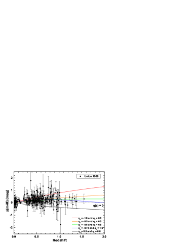
In Figure 1 we show the theoretical predictions of the kinematic approach to the residual Hubble diagram with respect to an eternally coasting Universe model ($q(z)\equiv 0$). The different models are characterized by the selected values of $q_{0}$ and $q_{1}$, as depicted in the diagram. Let us consider the maximum likelihood that can be determined from a $\chi^{2}$ statistics for a given set of parameters $(H_{0},q_{0},q_{1})$. In what follows we investigate the bounds arising on the empirical $q(z)$ parameters and the probability of the redshift transition for each SNe type Ia sample. By marginalizing the likelihood function over the nuisance parameter, $H_{0}$, the contours and the probabilities of the transition redshift for each sample are readily computed.

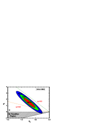
In Figure 2a, we see that the SCP Union sample strongly favors a Universe with recent acceleration ($q_{0}<0$) and previous deceleration ($dq/dz>0$). With two free parameter the confidence region is $0.7\leq q_{1}\leq 2.2$ and $-0.93\leq q_{0}\leq-0.52$ with ($68\%$) confidence level. It should be remarked the presence of a forbidden region forming a trapezium. The horizontal line in the top is defined by $q_{1}=0$ which leads to an infinite (positive or negative) transition redshift while the segment at $45^{o}$ is the infinite future ($z_{t}=-1$). The values of $z_{t}$ associated with the horizontal segment in the bottom are always smaller than -1 (no transition region), in fact $-1.5\leq z_{t}\leq-1$. Finally, one may conclude that the vertical segment is associated with $z_{t}\leq-1.5$, thereby demonstrating that the hachured trapezium is actually a physically forbidden region.

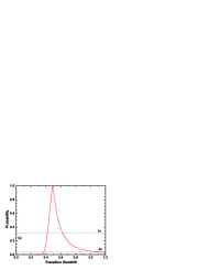
In Figure 2b (the center panel) one may see the probability of the associated transition redshift $z_{t}$, defined as $q(z_{t})=0$. It has been derived by summing the probability density in the $q_{0}$ versus the ${dq/dz}$ plane along lines of constant transition redshift, $z_{t}=-q_{0}/(dq/dz)$. The resulting analysis yields $z_{t}=0.49^{+0.135}_{-0.07}$ ($1\sigma$) ${}^{+0.54}_{-0.12}$ ($2\sigma$) for one free parameter which is in reasonable agreement with the value $z_{t}=0.46\pm 0.13$ Ries04 . In our analysis, the asymmetry in the probability of $z_{t}$ is produced by a partially parabolic curve obtained when $\chi^{2}$ is minimized. For this panel the central value $z_{t}=0.49$ does not agree with the cosmic concordance $\Lambda$CDM model in $68.3$% confidence level. However, it agrees with $95.4$% ($2\sigma$) for this approach. Note that $z_{t}=0.3$ ($z_{t}$ for flat $\Lambda$CDM with $\Omega_{m}\simeq\Omega_{\Lambda}\simeq 0.5$) is outside of the allowed region with $95\%$, while, $z_{t}=0.9$ (flat $\Lambda$CDM with $\Omega_{m}\simeq 0.2$ and $\Omega_{\Lambda}\simeq 0.8$) are well inside for the Union sample.

Table 1: Limits to the transition redshift $z_{t}$.

Sample (data)	$z_{t}$ (best-fit)	Confidence ($1\sigma$)	$\chi^{2}_{min}$
Gold 2004 (157)	$0.46$	$0.33\leq z_{t}\leq 0.59$	$176$
Astier 2006 (115)	$0.61$	$0.40\leq z_{t}\leq 4.29$	$113$
Gold 2007 (182)	$0.43$	$0.38\leq z_{t}\leq 0.52$	$156$
Davis 2007 (192)	$0.60$	$0.49\leq z_{t}\leq 0.88$	$195$
This paper (307)	$0.49$	$0.42\leq z_{t}\leq 0.63$	$310$

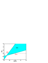
At this point it is interesting to investigate how our analysis constrains the redshift evolution of the decelerating parameter itself. The basic results are displayed in Fig. 2c, we see the evolution of the decelerating parameter as a function of the redshift for the parametrization $q(z)=q_{0}+q_{1}z$. The shadowed region denotes the 2$\sigma$ region. The data favor the recent acceleration ($q_{0}<0$) and past deceleration ($q_{1}>0$) with high confidence level.

It is also interesting to compare the results derived here with another independent analyses. The first constraints using this parametrization was obtained by Riess and collaborators from 157 SNe the transition redshift was constrained to be at $z_{t}=0.46\pm 0.13$ Ries04 . More recently, using 182 SNe Riess et al. obtained $z_{t}=0.43\pm 0.07$ for the probability density in the $q_{0}$ vs. $q_{1}$ plane along lines of constant transition redshift Riess07Lowas08 . In an early paper, we studied this parametrization to three samples. For Astier data set 2006 we obtained $z_{t}=0.61^{+3.68}_{-0.21}$, Gold sample 2007 the constraints were $z_{t}=0.43^{+0.09}_{-0.05}$, and Davies data set 2007 $z_{t}=0.60^{+0.28}_{-0.11}$. The asymmetries in our errors preserve the asymmetries in the $\chi^{2}$ analysis CunLim08 . Besides that, Bayesian analysis was implemented to study this kinematic scenario by Elgarøy and Multamäki ElgaMult06 , and, a kinematical study from type Ia supernovae and X-ray cluster gas mass fraction measurements, by combining them they obtain significantly tighter results than using the SNe sample alone Rapetti07 .

In Table 1 we summarize the recent results to the transition redshift $z_{t}$ in the kinematic approach derived from different samples of SNe Ia data. As shown there, for phenomenological law $q(z)=q_{0}+q_{1}z$ the limits were derived separately for each sample of SNe type Ia data.

IV Conclusions

In this paper we have discussed the transition redshift obtained from a kinematical approach within a flat FRW standard line element. Our study strongly favors a Universe with recent acceleration ($q_{0}<0$) and previous deceleration ($dq/dz>0$) for an analysis which is independent of the matter-energy content of the Universe based on the phenomenological law, $q(z)=q_{0}+q_{1}z$, and the SCP data compilation Kowalski08 . In our analysis we use the analytical expression to the distance luminosity CunLim08 , as well as, the excluded regions with $z_{t}<-1$ (figure 2a).

The likelihood function for the transition redshift was also discussed. In this case, the confidence regions in the bidimensional space parameter ($q_{0},q_{1}$) do not cross the physically forbidden region. Our analysis provides an independent evidence for a dynamical model in which a kinematic transition phase deceleration/acceleration happened at redshifts smaller than unity. Hopefully, the constraints on $z_{t}$ will be considerably improved in the near future with the increasing of supernova data at intermediate and high redshifts.

References

- (1) A. G. Riess et al., Astron. J. 116, 1009 (1998); S. Perlmutter et al., Astrophys. J. 517, 565 (1999); P. Astier et al., Astron. Astrophys. 447, 31 (2006); A. G. Riess et al., Astrop. J. 659, 98 (2007).
- (2) M. Kowalski et al., Astrophys. J. 686, 749 (2008).
- (3) R. C. Santos, J. V. Cunha and J. A. S. Lima, Phys. Rev. D 77, 023519 (2008), arXiv:0709.3679; R. C. Santos and J. A. S. Lima, Phys. Rev. D 77, 083505 (2008), arXiv:0803.1865.
- (4) T. Padmanabhan, Phys. Rep. 380, 235 (2003); P. J. E. Peebles and B. Ratra, Rev. Mod. Phys. 75, 559 (2003); J. A. S. Lima, Braz. Journ. Phys., 34, 194 (2004), [astro-ph/0402109]; E. J. Copeland, M. Sami and S. Tsujikawa, Int. J. Mod. Phys. D 15, 1753 (2006).
- (5) W. Chen and Y-S. Wu, Phys. Rev. D 41, 695 (1990); J. C. Carvalho, J. A. S. Lima and I. Waga, Phys. Rev. D 46, 2404 (1992); J. C. Carvalho and J. A. S. Lima, Gen. Rel. Grav. 26, 909 (1994); A. I. Arbab and A. M. M. Abdel-Rahman, Phys. Rev. D 50, 7725 (1994); J. A. S. Lima and J. M. F. Maia, Phys. Rev D 49, 5597 (1994); J. A. S. Lima and M. Trodden, Phys. Rev. D 53, 4280 (1996),[astro-ph/9508049]; J. A. S. Lima, Phys. Rev. D 54, 2571 (1996), [gr-qc/9605055]; M. V. John and K. B. Joseph, Phys. Rev. D 61, 087304 (2000); J. V. Cunha, J.A.S. Lima and N. Pires, Astron. Astrophys. 390, 809 (2002), [astro-ph/0202217]; M. K. Mak, J.A. Belinchon, and T. Harko, Int. J. Mod. Phys. D 11, 1265 (2002); M. R. Mbonye, Int. J. Mod. Phys. D 18, 811 (2003); J. V. Cunha and R. C. Santos, Int. J. Mod. Phys. D 13, 1321 (2004), [astro-ph/0402169]; I. L. Shapiro, J. Sola and H. Stefancic, J. Cosmol. Astropart. Phys. 0501, 012 (2005).
- (6) B. Ratra and P. J. E. Peebles, Phys. Rev. D 37, 3406 (1988); R. R. Caldwell, R. Dave and P. J. Steinhardt, Phys. Rev. Lett. 80, 1582 (1998); T. D. Saini et al., Phys. Rev. Lett. 85, 1162 (2000); J. A. S. Lima and J. M. F. Maia, Phys. Rev. D 65, 083513 (2002); F. C. Carvalho et al., Phys. Rev. Lett. 97 081301 (2006), [astro-ph/0608439]; L. Samushia and B. Ratra, Astrophys. J. 680, L1 (2008).
- (7) M. S. Turner and M. White, Phys. Rev. D 56, R4439 (1997); T. Chiba, N. Sugiyama and T. Nakamura, Mon. Not. R. Astron. Soc. 289, L5 (1997); J. A. S. Lima and J. S. Alcaniz, Astron.Astrophys. 357, 393 (2000), astro-ph/0003189; J. S. Alcaniz, J. A. S. Lima and J. V. Cunha, Mon. Not. Roy. Astron. Soc. 340, L39 (2003), [astro-ph/0301226].
- (8) A. Kamenshchik, U. Moschella and V. Pasquier, Phys. Lett. B 511, 265 (2001); M. C. Bento, O. Bertolami and A. A. Sen, Phys. Rev. D 66, 043507 (2002); M. C. Bento, O. Bertolami and A. A. Sen, Phys. Rev. D 67, 063003 (2003); J. V. Cunha, J. S. Alcaniz and J. A. S. Lima, Phys. Rev. D 69, 083501 (2004). J. A. S. Lima, J. S. Alcaniz, J. V. Cunha, Astropart. Phys. 30, 196 (2008) [arXiv:astro-ph/0608469].
- (9) G. Efstathiou, Mon. Not. Roy. Astron. Soc. 310, 842 (1999); J. V. Cunha, L. Marassi and R. C. Santos, Int. J. Mod. Phys. D 16, 403 (2007).
- (10) R. R. Caldwell, Phys. Lett. B 545, 23 (2002); J. A. S. Lima, J. V. Cunha and J. S. Alcaniz, Phys. Rev. D 68, 023510 (2003); P. F. Gonzalez-Diaz, Phys. Rev. D 68, 021303 (2003); Y.S. Piao and E. Zhou, Phys. Rev. D 68, 083515 (2003); J. A. S. Lima and J. S. Alcaniz, Phys. Lett. B 600, 191 (2004); G. Izquierdo and D. Pavón, Phys. Lett. B 633, 420 (2006). J. A. S. Lima and S. H. Pereira, Phys. Rev. D 78, 083504 (2008), arXiv:0801.0323; S. H. Pereira and J. A. S. Lima, Phys. Lett. B 669, 266 (2008), arXiv:0806.0682; N. Bilić, Fortschr. Phys. 56, 363 (2008), [arXiv:0806.0642].
- (11) M. S. Turner and A. G. Riess, Astrophys. J. 569, 18 (2002).
- (12) S. Weinberg, Cosmology and Gravitation(John Wiley Sons, New York, 1972).
- (13) C. L. Gardner, Nucl. Phys. B 707, 278 (2005)
- (14) J.-M. Virey et al., Phys. Rev. D 72, R061302 (2005).
- (15) Y. Gong and A. Wang, Phys. Rev. D 75, 043520 (2007).
- (16) E. E. O. Ishida et al., Astropart. Phys. 28, 547 (2008).
- (17) J. V. Cunha and J. A. S. Lima, Mon. Not. R. Astron. Soc. 390, 210 (2008), arXiv:0805.1261.
- (18) E. Mortsell and C. Clarkson, arXiv:0811.0981; C. Clarkson, B. Bassett and T. H.-C. Lu, Phys. Rev. Lett. 101, 011301 (2008).
- (19) E. Komatsu et al. (WMAP Collaboration), arXiv:0803.0547.
- (20) A. G. Riess et al., Astrophys. J. 607, 665 (2004).
- (21) A. G. Riess et al., Astrophys. J. 659, 98 (2007).
- (22) Ø. Elgarøy and T. Multamäki, J. Cosmol. Astropart. Phys. 09, 002 (2006).
- (23) D. Rapetti et al., Mon. Not. Roy. Astron. Soc. 375, 1510 (2007).