Structure formation as an alternative
to dark energy and modified gravity
Abstract
Observations are inconsistent with a homogeneous and iso-tropic universe with ordinary matter and gravity. The universe is far from exact homogeneity and isotropy at late times, and the effect of the non-linear structures has to be quantified before concluding that new physics is needed. We explain how structure formation can lead to accelerated expansion, and discuss a semi-realistic model where the timescale of the change in the expansion rate emerges from the physics of structure formation.
1 Introduction
1.1 Three assumptions and a factor of 2
The early universe, at least from one second onwards, is well described by a model which is homogeneous and isotropic (up to linear perturbations) and has only ordinary matter and gravity. Here ordinary matter refers to matter with non-negative pressure and ordinary gravity is based on the four-dimensional Einstein-Hilbert action. However, predictions of such models disagree with observations of the late-time universe by a factor of two or so. The angular diameter distance to the last scattering surface at a redshift of 1100 measured from the cosmic microwave background (CMB) is about 1.7 times smaller than in the spatially flat homogeneous and isotropic model dominated by pressureless matter. (Assuming that the primordial perturbations are adiabatic and that their spectrum is a power-law, and normalising to the same value of the Hubble parameter today.) Observations of type Ia supernovae and baryon acoustic oscillations at redshifts of order one and below are consistent with the CMB, and indicate that the discrepancy arises at late times, when the age of the universe is some billions of years.
In the context of the homogeneous and isotropic Friedmann-Robertson-Walker (FRW) models, there is a unique correspondence between the expansion rate and the distance scale (given the spatial curvature), and longer distances imply faster expansion. In terms of the expansion rate, compared to expectations, the Hubble parameter is a factor of 2 larger, given the observed energy density of matter (), or a factor of 1.2–1.5 larger, given the age of the universe ( 0.8–1 instead of ).
The factor 2 is observationally beyond reasonable doubt, so at least one of the three assumptions of the model is wrong. Either there is exotic matter with negative pressure (“dark energy”), or standard general relativity is not valid at large distances, or the universe is not homogeneous and isotropic, or some combination of the three.
There is no evidence for exotic matter or modified gravity apart from observations of the distance scale (and the related expansion rate). For example, modifications of gravity have not been observed in the solar system (apart from possibly the Pioneer anomaly) (Reynaud [2008]), and dark energy has not been measured in the laboratory. The situation is different from that of dark matter, for which there are several independent lines of evidence, such as the CMB peak structure, gravitational lensing, the rotation curves of galaxies, the motions of clusters, the early formation of structures and so on. In contrast, the various measurements of the distance scale (or the expansion rate) are probing the same physical observable using different tracers. An effect which increases the expansion rate (and correspondingly the distance scale) at late times can account for all of the observations.
Unlike the assumption of ordinary matter and gravity, the assumption that the universe is homogeneous and isotropy is known to be violated at late times, when non-linear structure formation has started. It is therefore necessary to quantify the effect of the breakdown of homogeneity and isotropy on the expansion rate before concluding that the observations call for new physics. It is suggestive that non-linear structures become significant at late times, when large departures from the predictions of the homogeneous and isotropic models with ordinary matter and gravity are observed. In contrast, models of exotic matter or modified gravity typically have no natural scale corresponding to billions of years, which is known as “the coincidence problem”.
In section 2 we explain how inhomogeneity and/or anisotropy can affect the expansion rate. In section 3 we discuss a toy model which helps to understand the physics of acceleration due to structure formation. In section 4 we discuss a semi-realistic model of structures, and demonstrate how the correct timescale of some billions of years emerges from the physics of structure formation. In section 5 we conclude with a summary. This is an overview of work reported in (Rasanen [2006a, 2006b, 2008a, 2008b]).
2 Backreaction
2.1 The fitting problem
The effect of inhomogeneity and/or anisotropy on the average expansion rate is known as backreaction. To be specific, consider a manifold which one can split into space and time. Take a fixed spatial domain and consider average quantities such as the energy density and the expansion rate in this domain. If the domain is inhomogeneous and/or anisotropic, the time evolution of these average quantities will be different than in a homogeneous and isotropic space, even if the initial conditions are the same.
One might expect the effects of inhomogeneities and/or anisotropies to be small in the real universe, since the universe looks homogeneous and isotropic when viewed on sufficiently large scales. However, one has to distinguish between exact and statistical homogeneity and isotropy. The early universe is locally close to exact homogeneity and isotropy, but after perturbations grow non-linear and structure formation starts, the universe is only statistically homogeneous and isotropic. In other words, the local evolution is non-linear, but the distribution of the non-linear regions is homogeneous and isotropic, with a homogeneity scale which is today of the order 100 Mpc (Hogg [2004]). A space which is only statistically homogeneous and isotropic expands differently than a locally homogeneous and isotropic space, since averaging and time evolution do not commute. This non-commutativity was first discussed in detail by George Ellis ([1984]), and he termed the issue of finding the model which best fits the average of the locally complex behaviour “the fitting problem”.
2.2 The local equations
It is possible to give some rather general results on the average expansion rate. Let us consider a general spacetime where the matter can be treated as dust, that is, a pressureless ideal fluid. After structure formation starts, this approximation does not hold (Pueblas & Scoccimarro [2008]), but the effects of velocity dispersion related to small scale structures are not expected to be important for our discussion. The geometry is determined by the Einstein equation
| (1) |
where is the Einstein tensor, is Newton’s constant, is the energy–momentum tensor, is the energy density and is the velocity of observers comoving with the dust.
We are interested in the average evolution of the geometry determined by (1). In curved spacetime, only scalars can be straightforwardly averaged, so we will look at the scalar part of (1). By taking the trace we obtain one scalar equation, and projecting with and gives two more (Buchert [1999]):
| (2) | |||||
| (3) | |||||
| (4) |
where a dot stands for derivative with respect to proper time measured by observers comoving with the dust, , is the expansion rate of the local volume element, is the scalar built from the shear tensor , is the scalar built from the vorticity tensor , and is the Ricci scalar on the tangent space orthogonal to the fluid flow. The equations are exact, and valid for arbitrary large variations in density, expansion rate and other physical quantities. The Hamiltonian constraint (3) is the analogue of the Friedmann equation, and gives the local expansion rate, and (4) expresses the conservation of mass. The Raychaudhuri equation (2) gives the local acceleration. In the FRW case, we would have and , where is the Hubble parameter.
We take the vorticity to be zero. While rotation is generated on small scales (Pueblas & Scoccimarro [2008]), we expect that vorticity, like velocity dispersion, is not important for the physics we discuss. Given , we see from (2) that the local acceleration is always negative (or at most zero). One might be tempted to conclude that since the local expansion decelerates everywhere at all times, the average expansion must also decelerate. However, this conclusion is false.
2.3 The Buchert equations
Let us see how the average expansion rate behaves by averaging the exact equations (2)–(4). This was first done by Thomas Buchert ([1999]). The average of a scalar quantity is simply its integral over the spatial hypersurface of constant proper time, divided by the volume,
| (5) |
where is the determinant of the metric on the hypersurface of constant proper time.
where the backreaction variable contains the effect of inhomogeneity and anisotropy:
| (9) |
and we have defined a scale factor such that the volume of the spatial hypersurface is proportional to ,
| (10) |
where has been normalised to unity at time , which we take to be today. As gives the expansion rate of the volume, this definition of is equivalent to . We will also use the notation .
The Buchert equations (6)–(8) differ from the FRW equations by the presence of the backreaction variable and the related fact that the spatial curvature is not necessarily proportional to . Because of this extra degree of freedom, the equations are not closed, but they provide a constraint on the expansion history. The backreaction variable in (9) has two parts. The shear is also present in the local equations (2)–(3), and acts to decelerate the expansion. The other term is the variance of the expansion rate, which has no counterpart in the local equations, and may in this sense be called emergent. This term expresses the non-commutativity of time evolution and averaging, and makes it possible for the average equations to have qualitatively different behaviour than the local equations. The contribution of the variance to the acceleration is always positive (except in the case of homogeneous expansion, when it is zero). If the variance is large enough compared to the contribution of the shear and the energy density, the average expansion rate accelerates, as (6) indicates, even though locally the expansion decelerates everywhere.
3 Demonstrating acceleration
3.1 A two-region toy model
The reason why the average expansion rate can increase even though the local expansion decelerates is simple. In an inhomogeneous space, different regions expand at different rates, and the volume of faster expanding regions increases more rapidly, by definition. Therefore the fraction of the volume which is expanding faster increases, and the average expansion rate can rise.
Structure formation in the universe starts from a density distribution which is very smooth, with only small local variations. In a simplified picture, overdense regions slow down as their density contrast grows, and eventually turn around and collapse to form stable structures. Underdense regions in turn become ever emptier, and their expansion rate increases (relative to the mean).
In order to clarify the physics of the acceleration due to inhomogeneity and/or anisotropy, we will consider a simple toy model of structure formation presented in (Rasanen [2006a, 2006b]), before discussing a semi-realistic model in the next section. We consider two spherical regions, one overdense and one underdense, with scale factors denoted by and , respectively. In the Newtonian regime, a spherically symmetric region expands like a FRW universe with the same mean density, regardless of the density profile. This is known as the spherical collapse model in the overdense case.
We take the underdense region, which models a cosmological void, to be completely empty, so it expands like . The evolution of the overdense region, which models the formation of a structure such as a cluster, is given by , , where the parameter is called the development angle. The value corresponds to the big bang singularity, from which the overdense region expands until , when it turns around and starts collapsing. The region shrinks to zero size at . In studies of structure formation, the collapse is usually taken to stabilise at due to vorticity and velocity dispersion, and we will also follow the evolution only up to that point.
The total volume in the toy model is . The average expansion rate and acceleration are
| (11) | |||||
| (12) |
where we have expressed the acceleration in terms of the deceleration parameter (note that negative corresponds to positive acceleration). The average expansion rate is the volume-weighted average of the expansion rates and , and it is therefore bounded from above by the fastest local expansion rate. In contrast, the acceleration is not simply the average of the local accelerations and . In addition to the first two terms in (12), which are the local values, there is a third term, which is non-positive, and contributes towards acceleration. This term depends on the difference of the expansion rates of the two regions, and corresponds to the variance part of the backreaction variable in (6).
(a)
(b)
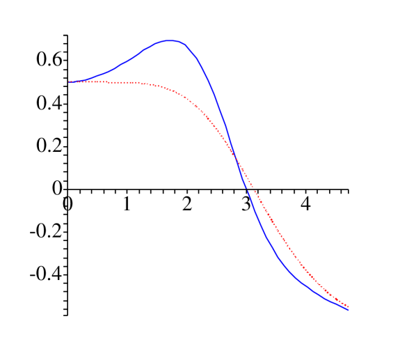
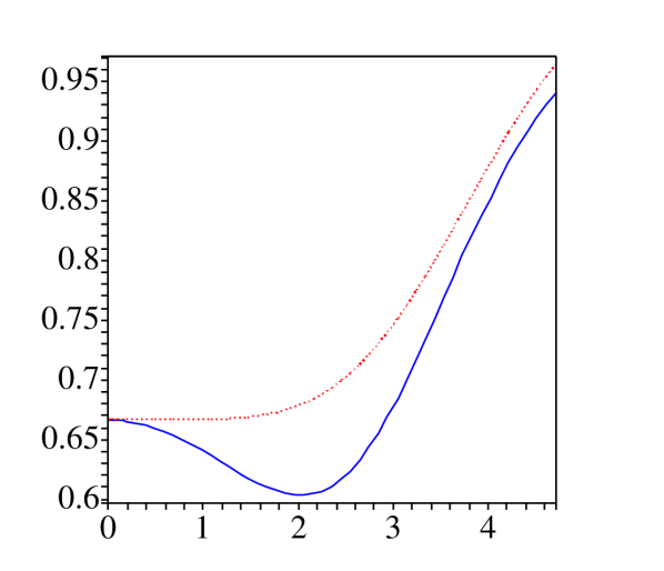
The toy model has one free parameter, the relative size of the two regions at some time. We fix this by setting the deceleration parameter to be equal to that of the spatially flat CDM FRW model when . In figure 1 (a) we plot as a function of the development angle . In addition to the toy model, we also show the CDM model for comparison. This is done to help understand the toy model, and does not imply that the toy model should be taken seriously in a quantitative sense.
The CDM model starts matter-dominated, with . As vacuum energy becomes important, the model decelerates less and then crosses over to acceleration. Asymptotically, approaches from above as the Hubble parameter approaches a constant. The toy model also starts with the FRW matter-dominated behaviour. As the overdense region slows down, the expansion decelerates more. Because the expansion of the overdense region is slower, the underdense region eventually takes over and comes to dominate the expansion rate. The expansion then decelerates less, and eventually accelerates; in fact the acceleration is stronger than in the CDM model.
The acceleration is not due to regions speeding up locally, but due to the slower region being less represented in the average. This is particularly easy to understand after the overdense region has started collapsing at . Then the contribution of the overdense region to (11) is negative, but the magnitude shrinks rapidly as decreases, so it is transparent that the expansion rate increases. Note that while there is an upper bound on the expansion rate, there is no lower bound on the collapse rate. Therefore, the acceleration can be arbitrarily rapid, and can even reach minus infinity in a finite time. (This simply means that the collapsing region is so dominant that vanishes in the denominator of .) This is in contrast to FRW models, where unless the null energy condition (or the modified gravity equivalent) is violated.
Figure 1 (b) shows the Hubble parameter multiplied by time as a function of the development angle . This is the same information as in figure 1 (a), but plotted in terms of the first derivative of the scale factor instead of the second derivative. In the CDM model, starts from in the matter-dominated era and increases monotonically without bound as approaches a constant. In the toy model, falls as the overdense region slows down, then rises as the underdense region takes over, approaching from below. The Hubble parameter in the toy model is at all times smaller than in the CDM model, and because is bounded from above by the fastest local expansion rate, cannot exceed unity. This bound is valid also in realistic models: as long as the matter can be treated as dust and vorticity can be neglected, inhomogeneous and/or anisotropic models predict , in contrast to FRW models with exotic matter or modified gravity. Observationally, 0.8–1.0 today (see section 5.1 of (Rasanen [2008a])).
Note that in an inhomogeneous and/or anisotropic dust model, whether the expansion accelerates simply depends on how rapidly faster expanding regions catch up with slower ones: roughly speaking, how steeply the curve rises. This is why the variance in (9) contributes to acceleration in the average Raychaudhuri equation (6). With a larger variance, the difference between slow and fast regions is bigger, and faster regions take over more rapidly.
4 Towards reality
4.1 A semi-realistic model of backreaction
The toy model shows that acceleration due to structure formation is possible, and helps to understand what this means physically. This possibility has also been demonstrated with the exact spherically symmetric dust solution, the Lemaître-Tolman-Bondi model (Chuang et al. [2005]; Kai et al. [2006]; Paranjape & Singh [2006]).
The issue is then whether this possibility is realised in the universe. The non-linear evolution of structures is too complex to follow exactly. However, because the universe is statistically homogeneous and isotropic, knowing some statistical properties is enough for evaluating the average expansion rate. In terms of the Buchert equations (6)–(8), the average expansion rate is completely determined once the variance and the shear are known. The average expansion rate is also determined if we know which fraction of the universe is in which state of expansion or collapse at each time. We will now discuss a semi-realistic model which does this by extending the two fixed regions of the toy model to a continuous distribution of regions which evolves in time (Rasanen [2008a, 2008b]).
The starting point is the spatially flat matter-dominated FRW model, with a linear Gaussian field of density fluctuations. Structures are identified with spherical peaks (and troughs) of the density field smoothed on some scale, following Bardeen ([1986]). The peak number density as a function of the smoothing scale and peak height can be determined analytically. We keep the smoothing threshold fixed such that , where is the root mean square density contrast, is time and is the smoothing scale. Non-linear structures typically form at , so corresponds to the size of the typical largest structures, and grows in time. The smoothing is just a simplified treatment of the complex stabilisation and evolution of structures in the process of hierarchical structure formation. Since the peaks are spherical and isolated, and they are individually assumed to be in the Newtonian regime, their expansion rate is the same as that of a FRW universe with the same density, as in the toy model. The fraction of volume which is not in peaks is taken to expand like the spatially flat matter-dominated FRW model.
The average expansion rate can be written as
| (13) |
where (or, more accurately, ) is the fraction of the volume in regions with linear density contrast and expansion rate . The correspondence between and is given by the spherical evolution model (i.e. the FRW evolution), and the distribution of regions is given by the peak statistics, which is determined by the power spectrum of the Gaussian density field. The power spectrum consists of the primordial spectrum, determined in the early universe by some process such as inflation, and the transfer function, which describes the evolution of the modes at later times.
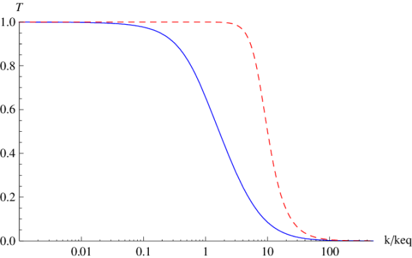
We take a scale-invariant primordial spectrum and the cold dark matter transfer function. For the latter, we consider two different approximations in order to show the uncertainty in the calculation. The BBKS transfer function (Bardeen [1986]) is a fit to numerical calculations (we take a baryon fraction of ), and the BDG form introduced by Bonvin et al. ([2006]) is a simple analytically tractable function with the correct qualitative features. In figure 2 we show the suppression of the amplitude of modes as a function of , the wavenumber divided by the wavenumber of the modes which enter the horizon at matter-radiation equality. The amplitude of modes which enter the horizon during the radiation-dominated phase is suppressed, while modes entering during matter domination retain their original amplitude. The only scale present in the model is the one associated with the turnover near matter-radiation equality. With the transfer function fixed, there are no free parameters: the expansion history given by (13) is completely fixed.
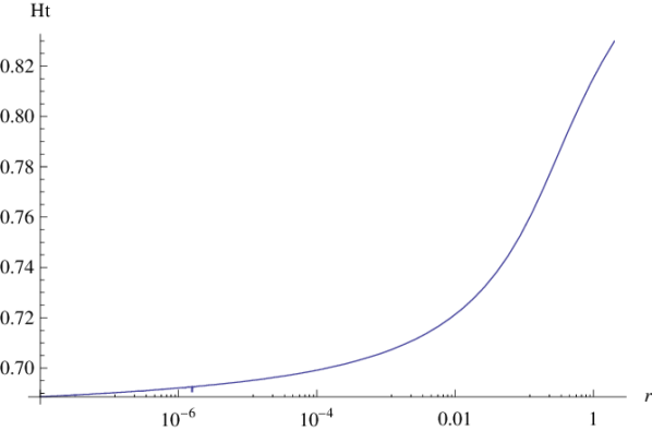
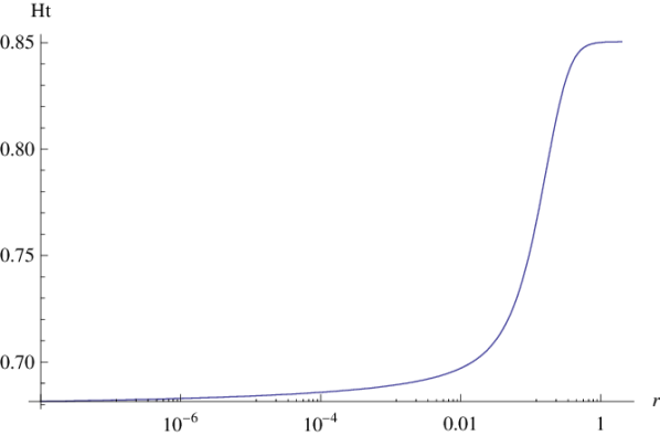
In figure 3 we show as a function of , the smoothing scale divided by the matter-radiation equality scale. As in the toy model, at early times. As time goes on, ever larger non-linear structures form, and they take up a larger fraction of the volume. The expansion rate grows (relative to the FRW value) slowly, until there is a rapid rise and saturation, roughly at the scale of matter-radiation equality. It is clear that after , when the perturbations which correspond to the matter-radiation equality scale collapse, must settle to a constant, since the transfer function is essentially unity, and there is no scale in the system anymore.
(a)
(b)
(a)
(b)
The matter-radiation equality scale is Mpc 100 Mpc, using the (somewhat model-dependent) value (Komatsu [2008]). Observationally, today on scales somewhat smaller than 8 Mpc, so 10 Mpc. Therefore the present day happens to be located around in the plots - exactly in the transition region.
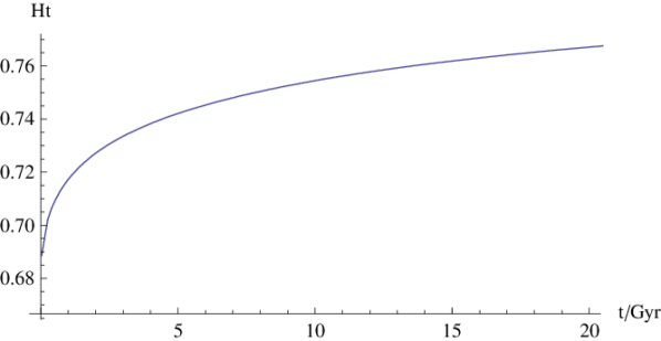
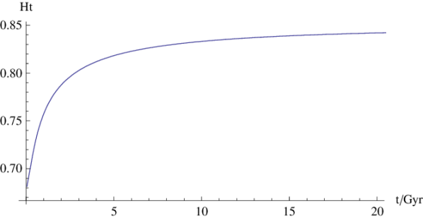
In figure 4 we show as a function of time (in billions of years) instead of the smoothing scale. The timescale is set by the matter-radiation equality time and the amplitude of the primordial density perturbations, . The matter-radiation equality time is years 50 000 years for . The primordial amplitude of the density perturbations inferred from the observations depends on the damping of the perturbations after deviations from the matter-dominated FRW evolution become important. We take the same amplitude as in the CDM model with today, (Dodelson [2003]). Ignoring damping by taking the matter-dominated FRW value would make the timescale longer by a factor of . The slope of the curve is less steep as a function of time than as a function of , because the size of structures grows more slowly at late times.
The timing of the rise of is remarkably close to the observed acceleration era, and the change is of the right order of magnitude, 15–25%. Nothing related to the present time has been used as an input in the model, the timing comes from the slope of the transfer function and the primordial amplitude.
As noted when discussing the toy model, acceleration is a quantitative question related to the slope of the curve. In the present case, while the expansion rate increases relative to the FRW case, the rise is not sufficiently rapid to correspond to acceleration. This is related to the fact that, unlike in the toy model, the overdense regions play almost no role, and the evolution of can be understood entirely in terms of the underdense voids. At early times, voids take up only a small fraction of the volume, and rises smoothly as they become prominent. In order for the change to be more drastic, the expansion rate should slow down due to overdense regions before the voids take over, as in the toy model.
The model involves a number of approximations, and it should not be trusted to more than an order of magnitude. For example, we have not taken into account in the statistics that peaks located inside larger peaks should not be double counted, and we should also exclude troughs which are inside peaks, while the reverse is not true (overdense regions can be located inside voids), which breaks the symmetry of the initial Gaussian density field (Sheth & van de Weygaert [2003]). Also, treating the peaks as isolated may not a good approximation once the peak density is high, collapsing structures are typically highly non-spherical, even the more accurate BBKS transfer function has an error of about 30% and so on. A more realistic calculation with quantified errors is necessary to estimate the effect of structures on the expansion rate in detail.
5 Conclusions
5.1 Summary
Observations are inconsistent with a homogeneous and isotropic universe with ordinary matter and gravity. FRW models do not include the effect of non-linear structures on the expansion rate. The Buchert equations, where the effect of structures is taken into account, show that the average expansion of a space can accelerate due to inhomogeneity and/or anisotropy.
With a simple toy model involving one overdense and one underdense region, we have demonstrated how acceleration is possible. First the expansion rate slows down due to the overdense region, and when the underdense region takes over, the change is sufficiently rapid that the expansion accelerates. The physical interpretation is simple: the fraction of volume in the faster expanding region grows, so the average expansion rate rises.
The important question is whether this happens in the real universe. We have discussed a semi-realistic model which involves an evolving distribution of regions, with statistics given by the peak number density of the initial Gaussian density field. In the model, the expansion rate rises at some billions of years by about 15–25%, the right order of magnitude. The physical reason is that the volume of the universe becomes dominated by voids. The model has no acceleration, because overdense regions are never prominent. This is not crucial, since the model is probably not correct beyond an order of magnitude, due to various approximations, such as the spherical symmetry of the structures and having equal amounts of mass in the overdense and underdense regions. It is remarkable that the correct timescale emerges from the physics of structure formation, essentially from the primordial amplitude of fluctuations and the time of matter-radiation equality imprinted on the cold dark matter transfer function. However, a more realistic calculation is needed to determine the details of the effect of structure formation on the expansion rate.
One important aspect which we have not discussed here is the relationship between the average expansion rate and observations of distance and redshift. Physically, it is clear that as the volume expands more rapidly, distances will grow longer. However, the quantitative relationship between the expansion rate and the distance scale remains to be determined (this is work in progress).
That structure formation could account for the observations of the late-time distance scale and expansion rate is a plausible possibility. Until the effect is quantified in detail, we do not know whether new physics is needed or the observations can be understood in terms of a complex realisation of general relativity.
References
- [1986] Bardeen, J.M., Bond, J.R., Kaiser, N. and Szalay, A.S., 1986 Astrophys. J. 304 15
- [2006] Bonvin, C., Durrer, R. and Gasparini, M.A., 2006 Phys. Rev. D73 023523 [arXiv:astro-ph/0511183]
- [1999] Buchert, T., 2000 Gen. Rel. Grav. 32 105 [arXiv:gr-qc/9906015]
- [2005] Chuang, C.H., Gu, J.A. and Hwang, W.Y., 2008 Class. Quant. Grav. 25 175001 [arXiv:astro-ph/0512651]
- [2003] Dodelson, S., 2003 Modern Cosmology, Academic Press, United States, p. 245
- [1984] Ellis, G.F.R., 1984, Relativistic cosmology: its nature, aims and problems, The invited papers of the 10th international conference on general relativity and gravitation, p. 215
- [2004] Hogg, D.W. et al., 2005 Astrophys. J. 642 54 [arXiv:astro-ph/0411197]
- [2006] Kai, T., Kozaki, H., Nakao, K.-i., Nambu, Y. and Yoo, C.M., 2007 Prog. Theor. Phys. 117 229 [arXiv:gr-qc/0605120]
- [2008] Komatsu, E. et al. [WMAP Collaboration], [arXiv:0803.0547 [astro-ph]]
- [2006] Paranjape, A. and Singh, T.P., 2006 Class. Quant. Grav. 23 6955 [arXiv:astro-ph/0605195]
- [2008] Pueblas, S. and Scoccimarro, R., [arXiv:0809.4606 [astro-ph]]
- [2008] Reynaud, S. and Jaekel, M.-T., [arXiv:0801.3407 [gr-qc]]
- [2006a] Räsänen, S., 2006 Int. J. Mod. Phys. D15 2141 [arXiv:astro-ph/0605632]
- [2006b] Räsänen, S., JCAP11(2006)003 [arXiv:astro-ph/0607626]
- [2008a] Räsänen, S., JCAP04(2008)026 [arXiv:0801.2692 [astro-ph]]
- [2008b] Räsänen, S., [arXiv:0805.2670 [astro-ph]]
- [2003] Sheth, R.K. and van de Weygaert, R., 2004 Mon. Not. Roy. Astron. Soc. 350 517 [arXiv:astro-ph/0311260]