Decoherence in rf SQUID Qubits

Abstract

We report measurements of coherence times of an rf SQUID qubit using pulsed microwaves and rapid flux pulses. The modified rf SQUID, described by an double-well potential, has independent, in situ, controls for the tilt and barrier height of the potential. The decay of coherent oscillations is dominated by the lifetime of the excited state and low frequency flux noise and is consistent with independent measurement of these quantities obtained by microwave spectroscopy, resonant tunneling between fluxoid wells and decay of the excited state. The oscillation’s waveform is compared to analytical results obtained for finite decay rates and detuning and averaged over low frequency flux noise.

1 Introduction

In the last few years there has been significant progress towards improved coherence times in superconducting qubits ither2005 ; steffen2006b ; martinis2005 ; choirescu2003 . However, progress has been slower in rf SQUID qubits then other similar devices such as phase qubits steffen2006b ; martinis2005 and persistent current qubits plantenberg2007 ; choirescu2003 ; saito2006 . This lack of improved coherence times is usually attributed to the larger size of rf SQUID devices which require a large loop (i.e. 150 $\mathrm{\ \mu m}$ x 150 $\mathrm{\ \mu m}$) to provide the necessary geometrical inductance. This paper will report recent measurements of coherence times of a modified rf SQUID, including Rabi oscillations, that suggest that the dominant source of decoherence in these devices is low frequency flux noise from two level fluctuators as seen in other superconducting qubits. We propose taking advantage of the sensitivity of rf SQUIDs to low frequency flux noise to investigate the source of the flux noise in the local environment.

An rf SQUID qubit in its simplest form consists of a superconducting ring of inductance $L$ interrupted by a single Josephson junction with critical current $I_{c}$ shunted by a capacitance $C$(see Fig. 1 inset). When a static external flux ($\Phi_{x}$) is applied to the SQUID loop, it induces a screening current $I_{s}=-I_{c}\sin(2\pi\Phi/\Phi_{0})$ where $\Phi_{0}\equiv\frac{h}{2e}$ is the flux quantum. The screened flux linking the loop ($\Phi$) must satisfy, $\Phi=\Phi_{x}+LI_{s}$. The dynamics of this device is analogous to a particle of mass C with kinetic energy $\frac{1}{2}C\dot{\Phi}^{2}$ moving in a potential given by the sum of the loop’s magnetic energy and the Josephson junctions coupling energy. Expressing the fluxes in units of $\Phi_{0}$, this potential is friedman2000

$$U(\phi,\phi_{x})=U_{0}\left[2\pi^{2}(\phi-\phi_{x})^{2}-\beta_{L}\cos(2\pi\phi)\right],$$ (1)

where $U_{0}\equiv\Phi_{0}^{2}/4\pi^{2}L$, $\beta_{L}\equiv 2\pi LI_{c}/\Phi_{0}$. Lowercase ($\phi_{\_\_}$) is used to denote the various fluxes in units of $\Phi_{0}$ (e.g. $\phi_{x}=\Phi_{x}/\Phi_{0}$). For $1<\beta_{L}<4.6$ and $\phi_{x}$ near $1/2$, the potential, shown in Fig. 1, has the form of a double well with the two wells representing different fluxoid states of the rf SQUID and having screening currents (of equal magnitude at the symmetry point, $\phi_{x}=1/2$) circulating in opposite directions around the loop friedman2000 . Changing $\phi_{x}$ has the effect of tilting the double well potential. One can select either the lowest level in each well or the two lowest levels in a single well for the basis states of the qubit. Since the two states have an easily measurable flux difference in the double well basis, this is referred to as the flux basis and requires a relatively low barrier to provide adequate coupling between the states. The single well mode, where the basis states are coupled by microwave radiation, on the other hand, requires a relatively high barrier so that the basis states do not couple to the states in the other well. This mode of operation is very close the that of qubits commonly referred to as “phase” qubits, so we will use this term to identify it. Figure 2 shows an example of calculated energy levels for the potential as a function of $\phi_{x}$. As can be seen, changes in $\phi_{x}$ cause a much greater change (about $100\times$) in the level spacing for the flux basis than for the phase basis. Since, as we shall see, there is substantial noise in $\phi_{x}$, this gives a strong advantage to the phase basis in terms of coherence times.

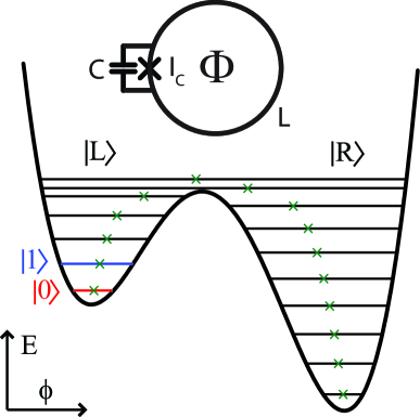
Figure 1: (Color online) The potential of an rf-SQUID at a $\beta=1.32$ and $\phi_{x}=0.505$ showing localized energy levels and the corresponding value of mean flux (green x). The inset shows a schematic representation of an rf SQUID

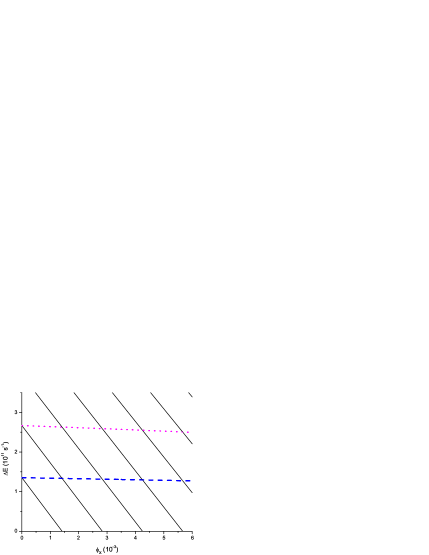
Figure 2: (Color online) The energy levels of the rf SQUID referenced to the lowest energy level in the left well. The blue dashed line (magenta dotted line) is the first (second) excited state localized in the left well. The black lines are the levels localized in the right well.

2 Design and Fabrication of the Qubit and On-Chip Control and Read-Out Circuitry

The qubits used in this work, shown schematically in the bottom center of Fig. 3(a), are enhanced versions of the simple qubit discussed above. This design uses a gradiometric configuration to help isolate the qubit from fluctuations in the ambient flux on the length scale (150 $\mathrm{\mu m}$) of the qubit, but can still be described by the simple potential of Eq. 1. If a single flux quantum were trapped in the outer loop when the qubit cooled through its transition temperature, then the motion of the system between the two wells of the potential would correspond to motion of the flux from the upper to lower loop of the gradiometer through the junctions connecting these two loops. If the ambient flux were zero, this situation would also result in the qubit potential being symmetric without further bias flux.

As noted above, different modes of operation of the qubit requires changes in the barrier height. It would, therefore, be very convenient to be able to adjust the height of the barrier of the double well potential, in situ, independently of $\phi_{x}$. This requires the ability to vary the critical current of the Josephson junction coupling the two wells. The twin requirements of low capacitance and rapid modulation using small control currents mean that a single large area junction cannot be used for this purpose. However, the critical current can be adjusted if the single junction is replaced by two junctions, with critical currents $I_{c1}$ and $I_{c2}$, in a small loop, a dc-SQUID, with inductance $\ell$ as shown in Fig. 3(a). By applying a flux, $\phi_{xdc}$, to this small loop the critical current of the dc-SQUID is suppressed allowing the barrier of the double well potential to be modulated. The addition of a second junction formally makes the potential two dimensional. However, if $L\gg\ell$ and $I_{c1}\approx I_{c2}$, then this 2D potential is very well approximated by the one dimensional potential in Eq. 1 with small corrections han1992 ; han1989 which can be neglected. $\beta_{L}$ is now given by $\beta_{L}(\phi_{xdc})=\beta_{L0}\cos(\pi\phi_{xdc})$ where $\beta_{L0}\equiv 2\pi L(I_{c1}+I_{c2})/\Phi_{0}$.

The flux $\phi_{x}$ that tilts the potential has both a low frequency component, $\phi_{x\ell f},$ that is applied using the on-chip gradient coil shown at the bottom right of Fig. 3(a) and high frequency components, discussed below in sec. III. The gradiometric design of the qubit has the further advantage that, to first order, there is no cross-coupling between the tilting flux, $\phi_{x\ell f},$ and the barrier modulation flux, $\phi_{xdc}.$ The outer loop of the $150$ $\mathrm{\mu m}$ $\times$ $150$ $\mathrm{\mu m}$ qubit is a 5 $\mu m$ wide Nb film with a thickness of 150 nm as is the film separating the two halves of the gradiometer except the thickness is 200 nm. This gives an effective qubit inductance of $L\approx 215$ pH. The dc-SQUID loop is $5$ $\mathrm{\mu m}$ $\times$ $5$ $\mathrm{\mu m}$ giving $\ell\approx 10$ pH. These inductances are calculated using the 3D-MLSI software package khapaev2001 and are consistent with measurements.

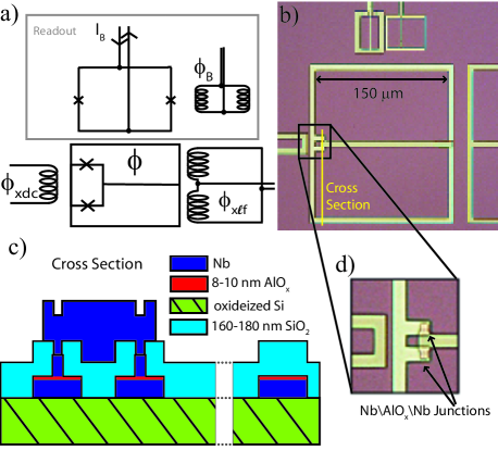
Figure 3: (Color online) (a) Schematic and (b) micrograph of an rf SQUID qubit and the readout magnetometer, (c) a cross section of the wafer around the junctions and (d) micrograph giving a detailed view of junctions.

The fluxoid state of the qubit is measured using a hysteretic dc SQUID magnetometer shown at the top of Fig. 3(a). The measured mutual inductance between the qubit and the magnetometer is 5 pH, consistent with the design value of 4.3 pH. The self inductance of the magnetometer is 56 pH and the junctions are 2.15 $\times$ 2.15 $\mathrm{\mu m}$ and 2.85 $\times$ 2.85 $\mathrm{\mu m}$ giving a maximum critical current of $10.8$ $\mathrm{\mu A}$. This asymmetric design, along with the asymmetry in the magnetometer flux bias loop, $\phi_{b}$, is part of a scheme to decouple the magnetometer bias leads from the qubit to first order while permitting fast triggering of the readout.

These circuits are fabricated at Stony Brook in our laboratory using a niobium trilayer process called the“SAL-EBL” process patel2005 ; chen2004 . This process has been developed from our well established planarized process for Nb superconducting electronics – the PARTS-EBL process patel1999 . The SAL-EBL process was developed specifically to study effects of various process steps on coherence in Nb based qubits. In particular, to maximize junction and film qualitypatel2005 ; pottorf08 and to minimize the turn-around time only essential process steps were retained, eliminating CMP (chemical mechanical polishing) and reducing process steps such as reactive ion etches (RIE) known to reduce film quality under certain conditionschen2003 . The resulting process has only one RIE step and uses a self-aligned lift-off (SAL) of the dielectric to define the junctions. By using lift-off for majority of the patterning, the process allows material flexibility for dielectric and wiring metal, and by using a combination of deep UV and electron beam lithography (EBL) on the same resist layer at each step allows great design flexibility.

The devices are fabricated on 2” oxidized Si wafers. The $\mathrm{Nb/AlO_{x}/Nb}$ trilayer is patterned via lift-off. Both Nb and Al are dc sputtered in Ar and $\mathrm{AlO_{x}}$ is formed by thermal oxidation. The junctions defined by EBL on a negative resist are formed by RIE in $\mathrm{SF_{6}}$ gas with a minimum device size of 0.15 x 0.15 $\mathrm{\mu m^{2}}$. The high area uniformity of the junctions allow us to accurately control junction asymmetry. The same resist mask is used to lift off rf sputtered $\mathrm{SiO_{2}}$ dielectric. A Nb wiring layer is also patterned through lift-off. Fig. 3(c) shows a cross-section of a completed device indicating various layer thicknesses. The process turn-around time is approximately one week, and the use of EBL for all critical features enables rapid design changes.

The size for the qubit junctions vary depending on desired qubit parameters and is 1.45 x 1.45 $\mathrm{\mu m^{2}}$ for the data shown. The designed current density for these devices is 1 $\mathrm{\mu A/\mu m^{2}}$. Both the junction size and current density are measured on diagnostic chips and agree with designed values. In particular the measurements of electrical size from both current and resistance scaling are consistent with physical size of the junctions estimated from RIE undercut. The asymmetry of the junctions (1.6%) is extracted from fits to $\phi$ as function of $\phi_{x}$ and is small enough to justify the use of Eq. 1 bennettthesis .

3 Apparatus and Measurement Techniques

Two essential criteria for the measurement of qubit dynamics are that one be able to prepare and readout states of the qubit with a time resolution short compared to the decoherence time of the states being studied and that the qubit be very well isolated from its environment so that the decoherence time is not affected, e.g. by the measurement and control processes, while the qubit is undergoing coherent evolution. This section presents the approaches used to achieve these goals with nanosecond resolution for qubits using the phase basis, which is far less sensitive to low frequency noise in $\phi_{x}$.

The on-chip bias coils, discussed in Sec. 2, can apply fluxes of the order of $\Phi_{0}$ but are limited to frequencies of less than $100$ kHz. To achieve nanosecond timing resolution, a separate set of high frequency flux bias signals, a microwave ($\phi_{xrf}$) and a video ($\phi_{xp}$) pulse with lengths on the order of nanoseconds and sub-nanosecond rise times, are inductively coupled to the qubit via a hole in the ground plane of a well characterized microstrip transmission line bennett2007 on a separate chip suspended 25 $\mathrm{\mu m}$ above the qubit chip . These signals, while very fast, are limited in amplitude to several thousandth of $\Phi_{0}.$ This gives, for the total bias flux applied to the large loop of the qubit, $\phi_{x}=\phi_{x\ell f}+\phi_{xrf}+\phi_{xp}+\phi_{off},$ where $\phi_{off}$ is a constant that includes the ambient flux and the zero offset in $\phi_{x\ell f}$, which is taken to be 0 at the symmetry point of the potential. The desired state of the qubit is obtained from the initial ground state of the left well by applying one or more microwave and video pulses.

Since the magnetometer cannot distinguish between the two basis states in the phase basis, an intermediate step must be used for the readout of the qubit state. To accomplish this, at the moment readout is desired, a short pulse, $\phi_{xp},$ is applied to tilt the potential rapidly but adiabatically to reduce the tunneling barrier between wells. The barrier height during this tilt is about $1.1$ K for the excited state of the qubit giving a tunneling rate to the right well of about 10⁹ $\mathrm{s^{-1}}$ while the rate for the ground state is about a factor of 500 slower. Thus it is possible to clearly distinguish these two states by appropriate selection of the pulse length. After the end of the pulse, the system will be trapped in either the left well (ground state) or the right well (excited state) for at least $1$ s. Subsequent readout of the occupied well using the magnetometer will then reveal the state of the qubit when $\phi_{xp}$ was applied.

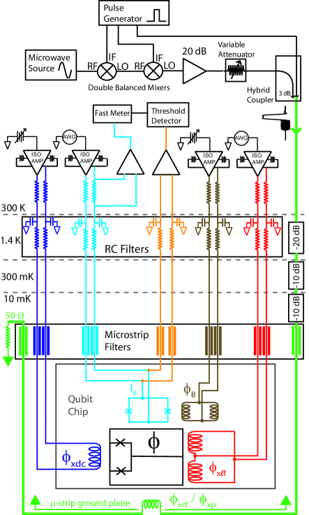
Figure 4: (Color online) Circuit schematic including the various stages of filtering and the components used to create and combine $\phi_{xrf}$ and $\phi_{xp}$.

The components that create and combine the microwave pulses and readout pulse are shown at the top of Fig. 4. The pulse generator is capable of producing measurement pulses with rise times as short as 200 ps. Two microwave mixers are used to modulate the envelope of the continuous microwave signal produced by the microwave source giving an on/off ratio of $10^{3}$. The output of the mixers is then amplified 20 dB and coupled through variable attenuators that set the amplitude of the microwave pulses applied to the qubit. Finally, these microwave pulses are combined with the video pulses using a hybrid coupler. The video pulses enter on the directly coupled port while the microwave pulse are coupled using the indirectly coupled port. The video pulses used for the data shown in the following sections are around typically 5 ns with a rise time of 0.5 ns. The directionality and frequency response of the coupler allows the two signals to be combined with a minimum amount of reflections and loss of power. This signal is then coupled to the qubit through a coaxial line that is filtered by a series of attenuators at 1.4 K (20 dB), 600 mK (10 dB) and at the qubit temperature (10 dB) followed by a lossy microstrip filter that cuts off around 1 GHz.

The low frequency bias and readout circuits for the qubit and magnetometer also have been optimized to control and measure the qubit while protecting it from noise. All signal paths are designed to be symmetric with respect to the chip to reduce the effect of common mode noise, and grounded signal sources are coupled through battery powered unity gain isolation amplifiers that effectively disconnect these signals from the earth ground. These low frequency lines are then filtered using EMI filters on entering the cryostat so that the dewar itself acts as an rf-shield for the cold portion of the experiment. They are further filtered using cascaded, 4-stage RC filters anchored at 1.4 K. Finally the lines are filtered using specially designed lossy microstrip filters at the qubit temperature.

Common RC filters are limited to about 1 GHz due to the parasitic inductance of the capacitor. The lossy microstrip filters were designed to cut off exponentially below 1 GHz and are effective to much higher frequencies. They consist of a thin film of chromium deposited on a glass or sapphire substrate and diced into long narrow chips. When the chips are placed in a brass housing, which acts as a ground plane, they form a lossy microstrip transmission line. The filters that must pass dc current also have a Nb meander line to pass the low frequency control currents without heating the filter assembly. These filters should be effective to the lowest order waveguide mode of the brass housing at 63 GHz while all other modes are greater then 500 GHz. At 18 GHz the microstrip filters have a measured attenuation greater than 95 dB.

The qubit chip and all the necessary wires and cables are housed in a superconducting NbTi sample cell that acts as a magnetic shield below its transition temperature around 10 K. This sample cell is mounted in the bottom section of a vacuum tight filter can, which has two chambers separated by an rf tight block housing the microstrip filters. This filter can is placed inside a double layer Cryoperm magnetic shield on the sample stage of a dilution refrigerator capable of reaching a loaded base temperature of 5 mK.

4 Results and Analysis

There are a number of different ways of characterizing the coherence times in our flux qubit. Experimentally, the simplest method of probing the decoherence involves measuring the lineshape of macroscopic resonant tunneling (MRT) between fluxoid statesrouse1995 . However the dynamics that determine the tunneling process are complicated, especially when the width of the peaks are not much smaller than the spacing between them. The measurement flux pulse discussed in the previous section makes it possible to measure the occupancy of the excited state and study intrawell dynamics. This along with controlled microwave pulses makes possible a direct measurement of the lifetime of the excited state and the observation of Rabi oscillations.

4.1 Lifetime of the Excited State

The decay rate between the first excited state and the ground state in the same well ($\Gamma_{1}$) provides an upper limit on the coherence time of the qubit in the phase basis. $\Gamma_{1}$ can be measured directly by measuring the occupation of the excited state, $\rho_{11}$, as a function of time. For this measurement, the qubit is pumped to the first excited state using a long microwave pulse followed by a measurement pulse $\phi_{xp}$ to read out the occupation of this state as a function of the delay, $\tau_{delay}$, between the end of the microwave pulse and the measurement pulse. A 80 ns microwave pulse, which is much longer than $T1\equiv$ $1/\Gamma_{1},$  is used in order to insure a constant initial mixture of the ground and excited state.

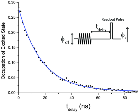
Figure 5: (Color online) The measured occupation of the excited state as a function of delay between the long microwave pulse and the readout pulse. The line is a fit to the exponential decay used to extract $T1$. The inset show the measurement pulse sequence.

Figure 5 shows the occupation of the excited state as a function of delay between the end of the microwave pulse and the readout pulse. The microwave frequency of 17.9 GHz is resonant with the energy difference between the ground and excited state for the value $\phi_{x\ell f}=0.050\times 10^{-3}$ used. The solid line is the fit to the data for $\rho_{11}\propto\exp(-\Gamma_{1}t)$ giving $\Gamma_{1}=0.05$ $\mathrm{ns^{-1}}$ or $T1=20$ ns. As we shall see below, such good fits are not always obtained for arbitrary bias.

The lifetime of the excited state is similar to lifetimes measured in a number of other $\mathrm{Nb/AlO_{x}/Nb}$ qubits operated in the phase basis (energy eigenstates in the same potential well). Paik et al. have observed decay times in dc SQUID phase qubits paik2007 around 13 ns for a $\mathrm{Nb/AlO_{x}/Nb}$ junctions and 20 ns for $\mathrm{Al/AlO_{x}/Al}$ junctions. Martinis et al. observed a lifetime of 20 ns in a large area current biased $\mathrm{Nb/AlO_{x}/Nb}$ Josephson junction martinis2002 . They were able to improve the lifetime to 500 ns martinis2005 through various changes including switching to Al junctions, reducing the size of the junction ($\sim 10$ $\mathrm{\mu m^{2}}$), and changing to $\mathrm{SiN_{x}}$ for the wiring insulation layer instead of $\mathrm{SiO_{2}}$.

4.2 Level Spectroscopy

If the decay with lifetime $T1$ were the dominant source of decoherence in the qubit, one would expect a resonance in the microwave occupation of the first excited state given, in the low power limit, by $\rho_{11}\propto\phi_{xrf}^{2}/(\delta^{2}+\Gamma_{1}^{2}/4)$ where $\delta$ is the mean difference between the photon energy and the level spacing. For the potential parameters used for the resonant data shown in Fig. 6 the dependence of $\delta$ on $\Phi_{x\ell f}$ is $\delta=1.70\times 10^{9}$ $\mathrm{s^{-1}/m\Phi_{0}}$. Measurement of the equilibrium occupation of the excited state near resonance is made using a readout pulse immediately following a 100 ns microwave pulse, which is much longer than the lifetime of the excited state as measured in Fig. 5, ensuring that the qubit reaches an equilibrium mixture of the ground and excited state. The detuning around the resonance is accomplished by changing $\phi_{x\ell f}$, rather than the frequency. This eliminates the effects of slight variations in $\phi_{xrf}$ as a function of the frequency. Figure 6 shows the occupation of the excited state for this potential as a function of $\delta$ for 3 different microwave power levels spaced by 3db, thus giving a factor of two total variation in $\phi_{xrf}$. For these values, the linewidth is nearly independent of $\phi_{xrf}$. So, one would expect the data to be in the low power limit with a linewidth given by $\Gamma_{1}$. As can be seen, however, the actual linewidth is about an order of magnitude greater, indicating additional noise broadening.

The effects of extra noise on this resonance between the ground and excited states within one well as well as on the resonant flux tunneling rate between levels in different wells (see Sec. 4.3) can both be described by a similar set of evolution equations for the density matrix.

In describing both types of resonant transitions between two levels, one needs to separate two types of interactions with the environmental noise. One is the decay, with the rate $\Gamma,$ of the excited state to the lower-energy states within the same well induced by the noise components at frequencies $\simeq\omega_{p}$. Another is due to the noise components at frequencies below $\omega_{p}$, which induce fluctuations of the energy difference $\nu(t)$ between the resonant levels. In the case of tunneling between the opposite wells, these fluctuations are induced directly by the energy shifts of one well relative to the other. For transitions within one well, both levels have practically the same value of average flux and the noise-induced fluctuations of the energy difference $\nu$ are much smaller, roughly by two orders of magnitude for the parameters of our qubits, than for the states in the opposite wells. We assume that the temperature $T$ of the environment is sufficiently large (this assumption is made more precise later in this Section, and in Sec. 4.4), so that the fluctuations $\nu(t)$ induced by the low-frequency part of the noise can be treated classically. In this case, evolution equations for the elements $\rho_{ij}$ of the density matrix in the basis of the two resonant states that account for both relaxation and the low-frequency noise can be written as (see, e.g., averin2000 )

$$\dot{\rho}_{11} =i\frac{a}{2}(\rho_{10}-\rho_{01})-\Gamma\rho_{11}\,,$$

$$\dot{\rho}_{00} =i\frac{a}{2}(\rho_{01}-\rho_{10})+\Gamma\rho_{11}\,,$$ (2)

$$\dot{\rho}_{01} =-i\nu(t)\rho_{01}-i\frac{a}{2}(\rho_{00}-\rho_{11})-\frac{\Gamma}{2}\rho_{01}\,,$$

$$\dot{\rho}_{10} =i\nu(t)\rho_{10}+i\frac{a}{2}(\rho_{00}-\rho_{11})-\frac{\Gamma}{2}\rho_{10}\,.$$

The coupling amplitude $a$ of the two states stands here for the tunnel amplitude $\Delta$ in the case of flux tunneling between the two wells, or for the microwave amplitude, $\phi_{xrf},$ expressed as the Rabi frequency $\Omega$ on resonance in the weak relaxation/dephasing limit (Sec. 4.4).

For microwave excitation of the first excited state in the well, $\Gamma$ is equal to the relaxation rate $\Gamma_{1}$ of this first excited state, and $\nu(t)$ in Eqs. (2) is the detuning between the excitation energy of this state and microwave frequency. If the low-frequency noise is negligible, $\nu(t)$ reduces to the average detuning $\delta$, and the steady-state occupation of the excited states is obtained from the stationary solution of the Eqs. (2) and has a Lorentzian line shape as a function of $\delta$:

$$\rho_{11}(\delta)=\frac{\Omega^{2}}{4\delta^{2}+2\Omega^{2}+\Gamma_{1}^{2}}.$$ (3)

If the cut-off frequency $\omega_{c}$ of the flux noise is much lower than the actual linewidth $W$ of the resonant transition, determined self-consistently by the rms value $u$ of the magnitude of the low-frequency noise and by the relaxation rate $\Gamma_{1}$ (see Eq. (4) below), the noise can be accounted for simply by convoluting the intrinsic Lorentzian lineshape (3) with some static distribution of the detuning values. Under a natural assumption of the Gaussian noise, this gives

$$\langle\rho_{11}\rangle=\frac{1}{\sqrt{2\pi}u}\int d\nu e^{-(\nu-\delta)^{2}/2u^{2}}\rho_{11}(\nu)\,.$$ (4)

In principle, the shape of the resonant peaks can provide information not only on the magnitude of noise but also on its spectral properties. For this, one needs to solve Eqs. (2) for the time-dependent $\nu(t)=\delta+\tilde{\nu}(t)$. This can be done analytically for the small microwave amplitude, $\Omega\ll W$, which can be treated as perturbation, i.e., when the contribution of $\Omega$ to the peak broadening (3) is negligible. Spectral properties of the stationary classical Gaussian noise are characterized by the correlator:

$$\langle\tilde{\nu}(t_{1})\tilde{\nu}(t_{2})\rangle=\frac{1}{2\pi}\int d\omega S(\omega)e^{i\omega(t_{1}-t_{2})}\,.$$ (5)

Perturbation theory in the coupling amplitude can be done directly in Eqs. (2) by integrating the equation for one of the off-diagonal elements of $\rho$ under the assumption that diagonal elements are constant, substituting then the result in the equations for the diagonal elements, and finally averaging the resulting transition rate over the Gaussian fluctuations of detuning using Eq. (5). This straightforward calculation gives

$$\langle\rho_{11}\rangle =\frac{\Omega^{2}}{2\Gamma_{1}}\int_{0}^{\infty}d\tau e^{-\Gamma_{1}\tau/2}\cos\delta\tau\times$$

$$\exp\{-\frac{1}{\pi}\int d\omega S(\omega)\frac{\sin^{2}\omega\tau/2}{\omega^{2}}\}\,.$$ (6)

This result is the limit of the classical noise, reached for large temperatures, $T\gg W$, of a more general quantum expression obtained in amin2008 . Qualitatively, the quantum component of the noise leads to a finite shift of the resonant peak position away from the zero-detuning point $\delta=0$ harris2008 . The shift disappears with increasing temperature $T$.

For noise with a Lorentzian spectrum:

$$S(\omega)=\frac{2u^{2}/\omega_{c}}{1+(\omega/\omega_{c})^{2}}\,,$$ (7)

Eq. (6) gives

$$\langle\rho_{11}\rangle =\frac{\Omega^{2}}{2\Gamma_{1}}\int_{0}^{\infty}d\tau e^{-\Gamma_{1}\tau/2}\cos\delta\tau\times$$

$$\exp\left\{-\frac{u^{2}}{\omega_{c}}\left(\tau-\frac{1-e^{-\omega_{c}\tau}}{\omega_{c}}\right)\right\}.$$ (8)

This equation describes the transition from the regime of the broadband noise, $\omega_{c}\gg W$, when the noise simply increases the linewidth $W$ of the Lorentzian (without the $\Omega$ in the denominator) to $\Gamma_{1}+2u^{2}/\omega_{c}$, to the regime of the quasistatic noise $\omega_{c}\ll W$, when the lineshape is given by Eq. (4), and for strong noise, $u\gg\Gamma_{1}$, is:

$$\langle\rho_{11}\rangle=\frac{\pi\Omega^{2}}{2\Gamma_{1}}\frac{1}{\sqrt{2\pi}u}e^{-\delta^{2}/2u^{2}}.$$ (9)

In the case of frequently assumed $1/f$ noise of amplitude $A$:

$$S(\omega)=\frac{A}{|\omega|}\,,$$ (10)

Eq. (6) always gives the quasistatic result (4) (with logarithmic accuracy) with $u^{2}\simeq(4A/\pi)\ln(W/\omega_{l})$, where $\omega_{l}$ is the lower cutoffs of the spectrum (10) roughly given by the time of one measurement cycle.

The lines in Fig. 6 are fits to the data for the microwave-induced occupation of the excited state, using Eq. 4 assuming extra low frequency flux noise noise in $\delta$ of rms amplitude $u=\sigma_{\nu}$ to obtain the lineshape. The best fit to the data, for all the powers shown, occurs for $\sigma_{\nu}=0.235\pm 0.01$ $\mathrm{ns}^{-1}$ and $\Gamma_{1}=0.055\pm 0.005$ $\mathrm{ns^{-1}}$. This analysis is based on the assumption that $\phi_{x}$ remains constant during the approximately $100$ ns time of a single measurement (the quasi-static approximation) suggesting that low frequency flux noise is indeed the dominant source of resonant broadening. As a test of the degree to which this fit actually tells us something about the frequency dependence of the noise, we refit the lowest peak in Fig. 6 using Eq. 8, which assumes Lorentzian noise with and arbitrary cutoff, $\omega_{c}$, but is valid only in the low power limit. The results of this are that the data can be fit almost as well for values of $\omega_{c}$ up to $2\times 10^{9}$ $\mathrm{s}^{-1}$ by increasing rms noise to $\sigma_{\nu}=0.28\pm 0.01$ $\mathrm{ns}^{-1}$. So it would seem that the fit provides very little information on the frequency dependence of the noise but gives a rather firm estimate of its amplitude.

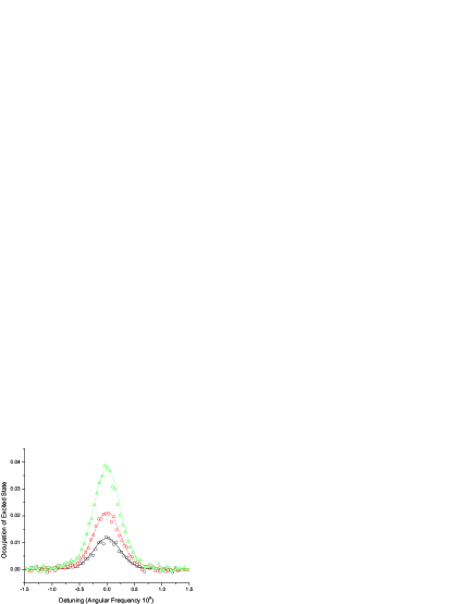
Figure 6: (Color online) The occupation of the excited state as a function of detuning for microwave powers corresponding to attenuator settings of 39 (squares), 36 (circles), 33 dB (triangles). Lines are fits using Eq. 4 at microwave amplitudes corresponding to the measured Rabi frequency for each attenuator setting (0.017, 0.024, 0.034 $\mathrm{ns^{-1}}$) with $\Gamma=0.055$ $\mathrm{ns^{-1}}$ convoluted with static Gaussian noise with $\sigma_{\nu}=0.235$ n$\mathrm{s^{-1}}$ at the angular frequencies of the Rabi oscillations that correspond to these microwave powers

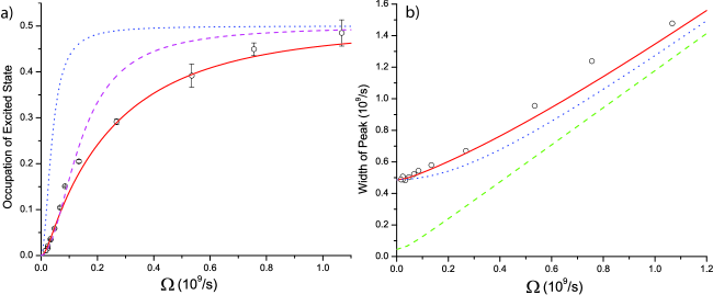
Figure 7: (Color online) (a) The occupation of the excited state on resonance versus microwave amplitude in units of the corresponding Rabi frequency. The lines are calculations for the following parameters; red solid $\Gamma=0.055$ $\mathrm{ns^{-1}}$ and $\sigma_{\nu}=0.235$ n$\mathrm{s^{-1}}$, blue dotted line $\sigma_{\nu}=0$ with $\Gamma=0.055$ $\mathrm{ns^{-1}}$, purple dashed line $\sigma_{\delta}=0$ and $\Gamma=0.20$ $\mathrm{ns^{-1}}$. (b) The width of the spectroscopic peak from the Gaussian fits as a function of microwave amplitude in units of Rabi frequency. The lines are calculations for the following parameters; red solid $\Gamma=0.055$ $\mathrm{ns^{-1}}$ and $\sigma_{\nu}=0.235$ n$\mathrm{s^{-1}}$, green dashed line $\sigma_{\nu}=0$ with $\Gamma=0.055$ $\mathrm{ns^{-1}}$, blue dotted line $\sigma_{\nu}=0$ and $\Gamma=0.585$ $\mathrm{ns^{-1}}$.

These fits can be extended to higher rf amplitudes where power broadening is important using Eq. 4, as shown in Fig. 7(a), which shows the maximum occupation of the excited state as a function of microwave amplitude for a much wider range of $\phi_{xrf}$. The red solid line is a fit to the peak amplitudes ($\delta=0$) using the same fitting parameters as in Fig. 6. For comparison, the blue dotted line is calculated for no flux noise, i.e. $\sigma_{\nu}=0,$ and $\Gamma=0.055$ $\mathrm{ns}^{-1}$ while the purple dashed line is calculated for $\sigma_{\nu}=0$ and $\Gamma=0.20$ $\mathrm{ns}^{-1}$ which gives the best fit to the low power data without considering low frequency noise. The peak amplitude cannot be fit over the whole range of microwave amplitudes without including the low frequency noise. Figure 7(b) shows the width of the peaks as a function of $\phi_{xrf}$ for the same data and the red solid line the fit for the same parameters as above. The green dashed line is the width for $\Gamma=0.055$ $\mathrm{ns}^{-1}$ and the blue dotted line for $\Gamma=0.585$ $\mathrm{ns}^{-1}$ and no low frequency noise. Again, low frequency Gaussian noise is required in order to obtain a reasonable fit to the overall lineshape of the data.

As noted above, the data shown in Figs. 6 and 7 were obtained by changing $\phi_{x\ell f}$ over a narrow range near points where the spectrum was well behaved. In general, however, the spectrum is much more complex as can be seen in Fig. 8 showing the occupation of the excited state as function of both frequency and $\phi_{x\ell f}$ for $\beta_{L}=1.30$ for a much wider range of parameters. The color contours are proportional to occupation of the excited state, blue being lower occupation and red being the highest occupation (0.325). The curving ridge running diagonally from the top left to the bottom right corresponds the resonance between the ground and excited state. The black solid line shows the calculated difference between these states as a function of $\phi_{x}$, where $L$ and $C$ are fitting parameters consistent with simulations and measurements (not shown) of thermal escape rates, positions of resonant tunneling peaks and photon assisted tunneling peaks bennettthesis . The gaps in the excited state occupation along this line are consistent with coupling to two level fluctuators, e.g. in the dielectrics, that have also been observed by other groups investigating superconducting phase qubits simmonds2004 ; martinis2005 ; palomaki2007 . In general these gaps do not correspond to the bias values where the states in the left well align with excited states in the right (indicated by the black circles).

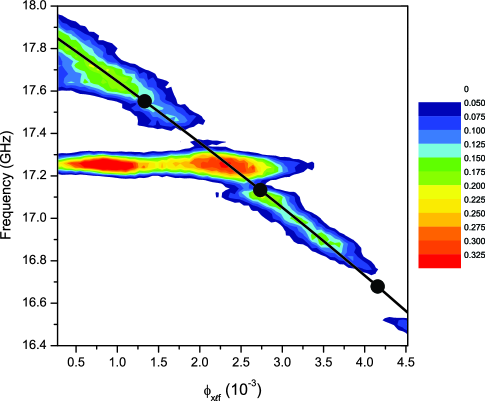
Figure 8: (Color online) The measured occupation of the excited state after a long microwave pulse expressed as color contours (blue being lowest and red being the highest) as function of both frequency and $\phi_{x}$. The solid lines are calculations of the energy level spitting between consecutive eigenstates states in the same well for $\beta=1.30$, $L=190$ pH and $C=210$ fF.

Another prominent feature in these data is the strong resonance near $17.25$ GHz over a wide range of $\phi_{x\ell f},$ which we attribute to a cavity resonance in the NbTi cell. The larger peak of this cavity resonance, to the left of the resonance between the ground and excited state, corresponds to a two photon resonance to the second excited state of the qubit. The frequency of this cavity resonance is in the range of the lowest order cavity modes of the sample cell, even though most of these modes should be suppressed due to the extremely small dimensions ($\sim 1$ mm) of the cell out of the plane of the chips.

These anomalous behaviors are further illustrated in Fig. 9(a), which shows the occupation of the excited state, using color contours, as a function of $t_{delay}$ and $\phi_{x\ell f}$. Here, the microwave frequency has been adjusted for each value of $\phi_{x\ell f}$ in order to remain on resonance. The bias value used for the measurement of the lifetime of the excited state shown in Fig. 5 is at the extreme left side of this plot.

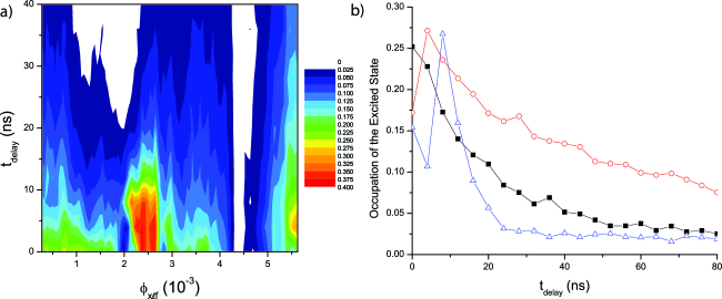
Figure 9: a) The measured occupation of the excited state after a long microwave pulse expressed as color contours (blue being lowest and red being the highest) as function $\phi_{x}$ and the delay between the end of the microwave pulse and the beginning of the readout pulse. b) Slices of the contour plot at $\phi_{x\ell f}=$ $0.767\times 10^{-3}$ (black squares), $2.078\times 10^{-3}$ (blue triangles) and $5.464\times 10^{-3}$ (red circles). The lines are just to help guide the eye.

At a number of bias points, the decay of the excited states is non-exponential, in contrast to the data of Fig. 5. For example, in the region near the gaps in the excitation spectrum, there are actually peaks in the occupation of the excited state as a function of $t_{delay}$. Figure 9(b) shows slices of Fig. 9(a) at $\phi_{x\ell f}=$ $0.767\times 10^{-3}$ (black squares), $2.078\times 10^{-3}$ (blue triangles) and $5.464\times 10^{-3}$ (red circles). At $\phi_{x\ell f}=$ $0.767\times 10^{-3}$ the decay is similar to that of Fig. 5, while for the other two $\phi_{x}$ values the behavior is clearly not exponential. The occupation of the excited state actually increases with time and reaches a local maximum at a non zero delay. At these bias points, it appears that the qubit is coupled strongly to a two level fluctuator as was reported by Cooper et al. cooper2004 in their investigation on current-biased phase qubits. They also observed an oscillation superimposed on the decay of the excited state near one of these splittings in the excitation spectrum.

4.3 Comparison with Resonant Tunneling Peaks

As noted above the same equations (with different parameters) that determine the shape of the spectroscopic peaks discussed above should also describe the resonance tunneling between levels in different wells of the potential as initially seen in experiments on MRT, where an enhancement of the escape rate from one well to the other was observed when the lowest energy level of the initial well approximately aligns with an energy level in the other. When the energy difference between the levels ($\varepsilon$) in opposite wells is much less than $\omega_{p}$ and the intrawell energy relaxation from the final state (the $n^{\text{th}}$ level of the right well) is $\Gamma_{n}$, this tunneling rate, which has a form analogous to Eq. 3, is given by averin2000

$$\Gamma_{esc}=\frac{\Delta^{2}\Gamma_{n}}{2\Delta^{2}+\Gamma_{n}^{2}+4\varepsilon^{2}}.$$ (11)

Away from resonance when the levels are localized in their respective wells, the escape rate can be approximated as the sum of the tunneling rates from the ground state in the left well ($|i\rangle$) to the lower energy states in the right well ($|f\rangle$). Assuming Ohmic dampening, this gives for the individual rates kopietz1988

$$\gamma_{{}_{i},_{f}}=\frac{2\pi}{\hbar}\frac{R_{Q}}{R}\left(E_{i}-E_{f}\right)\left|\langle i\left|\bm{\mathrm{\Phi}}\right|f\rangle\right|^{2},\text{ and }\Gamma_{esc}=\sum\gamma_{{}_{i},_{f}}$$ (12)

where R is the ohmic dampening, $R_{Q}\equiv h/4e^{2}$ is the quantum unit of resistance and $\bm{\mathrm{\Phi}}$ is the flux operator.

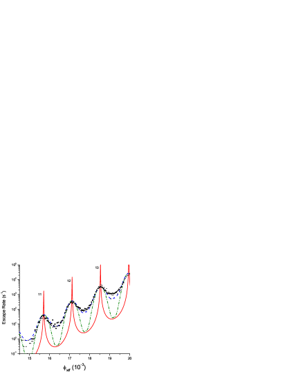
Figure 10: (Color online) Measured escape rates from the ground state in the left well as a function of $\phi_{x}$ at a $\beta=1.412$. The solid red line is a calculation for $\Gamma_{12}=0.68\operatorname{ns}^{-1}$. The green dash dot line corresponds to the solid line with the addition of static Gaussian noise with $\sigma_{\nu}=0.23\operatorname{ns}^{-1}$. The blue dashed line has the same level of Gaussian noise but with $\Gamma_{12}=10.5\operatorname{ns}^{-1}$.

These rates can be measured by pulsing $\phi_{x}$ from some initial value, where $\Gamma_{esc}$ in negligible to the tilt at which $\Gamma_{esc}$ is to be measured and leaving it there for some time $t_{m}$, in which the system has some reasonable probability of tunneling though the barrier into an excited state of the other flux well. Under the assumption above of incoherent tunneling, the system will then decay to the ground state of the new fluxoid well and remain trapped, so many repetitions of this measurement will give the probability of tunneling. The escape rate is determined from this probability of a transition, $P(\phi_{x})$, by

$$\Gamma_{esc}(\phi_{x})=\frac{1}{t_{m}}\ln\left(\frac{1}{1-P(\phi_{x})}\right).$$ (13)

The measured escape rates are shown in Fig. 10 as a function of $\phi_{x\ell f}$. The resonant tunneling peaks are labeled with an index that indicates which level in the right well is aligned with the ground state in the left well. The red solid line is a calculation of the escape rates using Eqs. 11 and 12 with the measured qubit parameters. The decay rate, $\Gamma_{12}=0.68$ $\mathrm{ns}^{-1}$ is the product of the decay rate directly measured in Section 4.1 and the level number ($n=12$). This calculation gives peaks much narrower than the measured peaks. The green dash dot lines are these same peaks convoluted with static Gaussian flux noise in analogy to Eq. 4 with $\sigma_{\nu}=0.235\pm 0.01$ $\mathrm{ns}^{-1}$, the same as the level of flux noise used to fit the spectroscopy in Sec. 4.2. For these parameters, the shape of the resonant tunneling peaks are well fit, but not the intervening valleys. In order to make both the peaks and valleys fit, the relaxation rate must be increased to $\Gamma_{12}=10.5$ $\mathrm{ns}^{-1}$ which is inconsistent with the measured $\Gamma_{1}$. It may well be that a more refined theory is needed for the tunneling minima between the peaks.

4.4 Time domain measurements

While the data in the previous sections, clearly show the effects of various processes leading to decoherence in the qubit and even provide a means to obtain qualitative estimates of the decoherence rates, they are all obtained from non-coherent processes. In order to demonstrate coherence in our qubit and to compare the resulting decoherence rates with those due to the know sources of decoherence discussed above, we now turn to time domain measurements of the evolution of coherent superpositions of the two qubit states.

An analytic solution to the Bloch equations for the population of the excited state in the presence of CW microwave, assuming no decoherence and that the system starts in the ground state at time zero, is given by

$$\rho_{11}(t,\delta)=\frac{\Omega^{2}}{\Omega^{2}+\delta^{2}}\sin^{2}(\Omega_{Rabi}(\delta)t/2),$$ (14)

where

$$\Omega_{Rabi}(\delta)=\sqrt{\delta^{2}+\Omega^{2}}.$$ (15)

This solution, shows that when driven with microwaves, the population of the excited states oscillates in time, demonstrating the phenomenon of Rabi oscillations, which have been seen in a number of different superconducting qubits nakamura1999 ; choirescu2003 ; vion2002 ; martinis2002 ; wallraff2005 . $\Omega,$ the frequency of the oscillations for $\delta=0,$ is ideally proportional to the amplitude of the microwaves excitation $\phi_{xrf}$ . This linear dependence is accurately seen in our qubit at low power levels (see Fig. 11 upper inset) providing a convenient means to calibrate the amplitude of the microwaves incident on the qubit in terms of $\Omega.$

The measurement sequence for coherent oscillations is very similar to that used to measure the lifetime of the excited state except that the duration of the (generally shorter) microwave pulse is varied and the microwave pulse is immediately followed by the readout flux pulse. This signal, on the high frequency line, is illustrated in the lower inset in Figure 11. Figure 11 shows an example of the Rabi oscillations when $\delta=0$ and the microwave frequency, $f_{xrf}=17.9\mathrm{GHz}$. This bias point lies in a ”clean” range of the spectrum ($17.6-18\mathrm{GHz})$ as seen in Fig. 8, which should be the best region for observing coherent oscillations between the ground and excited states. Most of the time domain data, including the lifetime measurements of Fig. 5, have been taken in this frequency range. Each data point in Fig. 8 corresponds to the average of several thousand measurements for a given pulse length.

4.5 Rabi Oscillations

In order to simulate the time dependent dynamics of the Rabi oscillations in the presence of the low-frequency noise, it is convenient to separate this noise in the two parts. One, the quasi-static part, consists on the noise components with frequencies smaller than the linewidth $W$ of the corresponding resonance. Under the conditions of the Rabi oscillations, $W$ is smaller than the strength $\Omega$ of coherent rf coupling between the two levels, which gives the Rabi oscillation frequency in the case of resonance ($\delta=0$) and weak relaxation/dephasing. This part of the noise can be taken into account by simple averaging over the static distribution of detuning $\delta$ as in Eq. 4. The second, “dynamic” part of the low-frequency noise has components with frequencies extending beyond $W$. We treat this noise making an assumption (relevant for the data presented in this work) that the temperature $T$ is larger than not only $W$, but also the Rabi frequency $\Omega$. In this case, it is possible to characterize this part of the noise as the classical noise with the same constant spectral density $S$ extending above $\Omega$ and equal to the spectral density at frequency $\Omega$. As discussed in Sec. 4.2, such a broadband noise simply increase the decoherence rate of the two states by $S/2$ (i.e., by $u^{2}/\omega_{c}$ in the example of Eq. (8) of that Section) to $\gamma=(\Gamma+S)/2$. With this modification of the decoherence rate, Eqs. (2) for the evolution of the density matrix of the two rf-coupled states can be written as

$$\dot{p} =\Omega v-\Gamma p-\Gamma/2\,,$$

$$\dot{u} =\delta v-\gamma u\,,\;\;\;\;\;\;$$ (16)

$$\dot{v} =-\delta u-\Omega p-\gamma v\,,$$

in terms of the imbalance $p=(\rho_{11}-\rho_{00})/2$ of the occupation probabilities $\rho_{00},\,\rho_{11}$ of the ground and excited state, and the real/imaginary parts $u,v$ of the off-diagonal element $\rho_{01}=u+iv$ of the density matrix. As Bloch equations (16) describe the dynamics of the Rabi oscillations, and are appropriate when the relaxation/dephasing rates are small on the scale of plasma frequency. The finite relaxation/dephasing rates make the analytic solution to these equations, which is shown below, considerably more complex than the undamped solution of Eq. 14.

Decaying Rabi oscillations described by Eqs. (16) lead to some stationary values of the occupation imbalance $p$ and coherences $u,v$ that are established after the decay of the oscillations. The analytic solution of Eqs. (16) that corresponds to this process can be written as:

$$A(t)=A_{st}+e^{-\gamma t}\sum_{j}e^{\lambda_{j}t}A_{j}\,,$$ (17)

where the “vectors” $A$ are composed of the elements (16) of the density matrix, $A=\{p,u,v\}$, and $A_{st}$ represents the stationary part of the solution:

$$A_{st}=\frac{-1/2}{\delta^{2}+\gamma^{2}+\Omega^{2}\gamma/\Gamma}\{\delta^{2}+\gamma^{2},\Omega\gamma,\Omega\delta\}\,.$$ (18)

The sum in Eq. (17) is taken over the three eigenvalues $\lambda_{j}$ of the evolution matrix $S$:

$$S=\left(\begin{array}[c]{ccc}\gamma-\Gamma&0&\Omega\\ 0&0&\delta\\ -\Omega&-\delta&0\end{array}\right),$$ (19)

which are given by the roots of the cubic equation $\mbox{det}(S-\lambda)=0$. In the range of parameters relevant for the present discussion (not very strong relaxation/dephasing) one root is real:

$$\lambda_{1}\equiv\lambda=s_{+}-s_{-}+(\gamma-\Gamma)/3\,,$$ (20)

and the other two are complex conjugated:

$$\lambda_{2}=\lambda_{3}^{\ast}\equiv\kappa+i\omega\,,\;\;\;\omega=\frac{\sqrt{3}}{2}(s_{+}+s_{-})\,,$$ (21)

$$\kappa=\frac{1}{2}(s_{-}-s_{+})+\frac{1}{3}(\gamma-\Gamma)\,,$$ (22)

where

$$s_{\pm}=\left[(q^{3}+r^{2})^{1/2}\pm r\right]^{1/3},$$ (23)

and

$$q =\frac{1}{3}(\Omega^{2}+\delta^{2})-\frac{1}{9}(\Gamma-\gamma)^{2},$$

$$r =\frac{\Gamma-\gamma}{3}\left(\frac{1}{2}\Omega^{2}-\delta^{2}-\frac{1}{9}(\Gamma-\gamma)^{2}\right)$$ (24)

The vectors $A_{j}$ in Eq. (17) are the projections of the vector $A(0)-A_{st}$ of the deviations of the initial elements of the density matrix from their stationary values, onto the eigenvectors of the evolution matrix (19) that correspond to the eigenvalues $\lambda_{j}$. These projections can be found conveniently from the following expression:

$$A_{j}=\frac{(S-\lambda_{k})(S-\lambda_{l})}{(\lambda_{j}-\lambda_{k})(\lambda_{j}-\lambda_{l})}[A(0)-A_{st}]\,,$$ (25)

which for each $j$, directly cancels out components of the two other eigenvector $k,l\neq j$ in the initial vector $A(0)-A_{st}$.

If the dynamics of the system starts at $t=0$ in the ground state, then $A(0)=\{-1/2,0,0\}$. In this case, using Eq. (18) for the stationary vector $A_{st}$ and the matrix $S$ (19) in the Eq. (25), together with the expressions for the eigenvalues $\lambda_{j}$ given above, we find the time dependence of the occupation probability $\rho_{11}$ of the excited state as

$$\rho_{11} =\frac{\gamma}{2\Gamma}\frac{\Omega^{2}}{\delta^{2}+\gamma^{2}+\Omega^{2}\gamma/\Gamma}\left[1-\frac{e^{-\gamma t}}{(\lambda-\kappa)^{2}+\omega^{2}}\right.$$

$$\Big{\{}e^{\lambda t}(\kappa^{2}+\omega^{2}-2\kappa\gamma+\gamma(\gamma-\Gamma)-\Omega^{2}-\delta^{2}\Gamma/\gamma)+$$

$$e^{\kappa t}\big{[}(\lambda(\lambda-2\kappa)+2\kappa\gamma-\gamma(\gamma-\Gamma)+\Omega^{2}+\delta^{2}\Gamma/\gamma)\times$$

$$\cos\omega t+[\omega^{2}(\gamma-\lambda)+(\kappa-\lambda)(\kappa\lambda-\gamma(\kappa+\lambda)+$$

$$\left.\gamma(\gamma-\Gamma)-\Omega^{2}-\delta^{2}\Gamma/\gamma)]\frac{\sin\omega t}{\omega}\big{]}\Big{\}}\right].$$ (26)

Equation (26) gives the decay rate of the Rabi oscillations as $\eta=\gamma-\kappa$. If the decay/relaxation rates in Eqs. (16) are small in comparison to $\Omega$, the rate $\eta$ reduces to the Rabi oscillations decay rate $\widetilde{\Gamma 2}$ obtained previously by Ithier et al. ither2005 , who expressed it in terms of the noise-induced decay rate at the Rabi frequency $\Gamma_{\nu}$ and the decoherence rate $\Gamma_{\phi}$ as

$$\widetilde{\Gamma 2}=\frac{1}{\delta^{2}+\Omega^{2}}\left[\frac{\Gamma}{4}\left(3\Omega^{2}+2\delta^{2}\right)+\delta^{2}\Gamma_{\phi}+\frac{\Gamma_{\nu}\Omega^{2}}{2}\right]\,.$$ (27)

As discussed above, at large temperature $T$, the noise is classical at the Rabi frequency, and one can take $\Gamma_{\nu}=\Gamma_{\phi}$. In this case, $\gamma=\Gamma/2+\Gamma_{\nu}$, and for weak relaxation/dephasing, the two Rabi decay rates agree, $\eta(\delta)=\widetilde{\Gamma 2}(\delta)$.

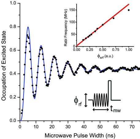
Figure 11: (Color online) The occupation of the excited state as a function of the length of the microwave pulse demonstrating Rabi oscillations. The line is a fit to Eq. 26 for $\delta=0$ averaged over quasi-static noise with $\sigma_{\nu}=0.22$ $\mathrm{ns}^{-1}$. This gives $f_{rabi}=119$ MHz and decay time $\widetilde{T2}=24$ $\mathrm{ns}^{-1}$. The upper inset shows Rabi frequency as a function of amplitude of applied microwaves in arbitrary units. The line is a linear fit to the lower microwave amplitude data. The lower inset show the measurement pulse sequence.

The data for resonant Rabi oscillations, shown in Fig. 11. The solid line is a fit using Eq. 26 including a $0.5$ ns time delay for the rise time for the microwave pulse and averaged over quasi-static Gaussian noise in $\phi_{x}$ equal to that obtained from the fits to the spectroscopy data in Fig. 6. This gives a Rabi frequency $f_{rabi}=119\mathrm{MHz}$ and decay rate, $\eta=0.042$ $\mathrm{ns}^{-1}$, for the oscillations. Equation 27, with $\delta=0$, together with our previously measured value for the decay rate of the first excited state $\Gamma_{1}$ (which gives the rate $\Gamma$ in the equations above), and the observed Rabi decay rate $\eta$ discussed below, imply $\Gamma_{\nu}=0.01$ $\mathrm{ns}^{-1}.$ Even though $\Omega_{Rabi}$ is not affected by flux noise to first order for $\delta=0,$ the amplitude of the flux noise in our qubit is large enough to cause a measurable effect. If the flux noise were neglected, it would be necessary to increase $\eta$ to $0.058$ $\mathrm{ns}^{-1}$ in order to account for the observed decay. In addition to increasing the decay rate, the low frequency noise also reduces the steady state occupation of the excited state, i.e. its value for long pulses, as calculated from Eq. 4. The ordinate of Fig. 6 has been calibrated using this value and is consistent with the estimate obtained  from the calculated tunneling rates from the two levels involved during the readout pulse.

The upper inset to Figure 11 shows the Rabi frequency extracted from Rabi oscillation measurements versus microwave amplitude in arbitrary units. As noted above, at low powers the Rabi frequency is linear in microwave amplitude as expected. At higher powers, however, it begins to saturate. There is evidence that at these higher power levels there is a small probability of excitation to the second excited state. However since the second excited state has orders of magnitude higher escape rate, this small probability can be significant.

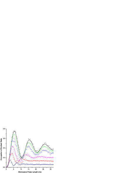
Figure 12: (Color online) Rabi oscillations for detunings going from top to bottom of 0.094, 0.211, 0.328, 0.562, 0.796 and 1.269 $\mathrm{ns^{-1}}$ with the corresponding fits using $\Gamma=0.075$ $\mathrm{ns^{-1}}$ and $\sigma_{\nu}=0.22\operatorname{ns}^{-1}$

The effects of flux noise on the decay of the Rabi oscillation, of course, becomes much more pronounced for $\delta\neq 0$. Figure 12 shows such Rabi oscillations at various detunings over a range of $0\leq\delta\lesssim 10^{9}$ $\mathrm{s}^{-1}$. At long microwave pulse times (not shown) the occupation of the excited state reaches the equilibrium values discussed in Sec 4.2. Near resonance, the value of $\rho_{11}$ for long pulse lengths is determined mainly by the noise amplitude, while for large $\delta$ it is set by $\delta.$ The data cannot be fit to solutions of the Bloch equations using only the phenomenological decay constants. As in the spectroscopy, static Gaussian detuning noise must be included to fit the data over the whole range of detuning. The lines in Figure 12 correspond to calculations with an initial Rabi frequency of $0.59$ n$\mathrm{s^{-1}}$, $\Gamma=0.075$ $\mathrm{ns^{-1}}$ and $\sigma_{\nu}=0.22$ $\mathrm{ns^{-1}}$. The detuning frequency is taken from $\phi_{x}$ using the conversion from Fig. 8. For the range of $\delta$ in Fig. 12 $\Delta E_{01}$ is in a region with relatively few spectral anomalies. However for $\delta<0$, on the other side of resonance towards splittings in the spectroscopy, the data generally do not agree with theory suggesting that the spectroscopic splittings have a strong effect on the coherence, as expected.

4.6 Ramsey Pulse Sequence

The effects of dephasing due low frequency flux noise should be seen most dramatically in the decay of Ramsey fringes. However the observation of Ramsey fringes in this system is complicated by the short lifetime of the excited state. To reduce these problems we have used the pulse sequence shown in Fig. 13(a). Here the $\pi/2$ pulses are applied on resonance and the detuning is produced in between these pulses, using an additional $\phi_{xp}$ pulse to tilt the potential and slightly change the level spacing for a variable time.

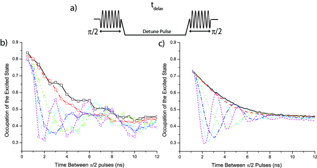
Figure 13: (Color online) (a) Measurement pulse sequence and (b) Measured occupation of the excited state after a series of 3 ns microwave pulses as a function of delay between the two pulses for various detuning pulse amplitudes (corresponding frequency); 0 V $\square$’s (no detuning), 0.1 V $\circ$’s (0.21 $\mathrm{ns^{-1}}$), 0.45 V $\vartriangle$’s (0.96 $\mathrm{ns^{-1}}$), 0.8 V $\triangledown$’s (1.70 $\mathrm{ns^{-1}}$), 1.15 V $\diamond$’s (2.45 $\mathrm{ns^{-1}}$) and 1.50 V $\triangleleft$’s (3.20 $\mathrm{ns^{-1}}$). (c) Calculations including noise for the pulse sequence by numerically solving the Bloch equations for the parameters corresponding to the measurement.

Figure 13(b) shows the measured occupation of the excited state as a function of delay between 3 ns microwave pulses (17.9 GHz) for several different values of detuning. The lines are provided to help guide the eye between the points. The expected Ramsey fringes can be calculated by numerically solving the Bloch equations, using a time dependent detuning along with the time dependent driving amplitude. As in previous sections, the resulting oscillations are convoluted with quasi-static Gaussian distributed noise. Figure 13(c) shows these calculated occupations of the excited state for the parameters corresponding to the data in Fig. 13(b). The scale factor for the amplitude of the detuning pulses was used as a fitting parameter but is consistent with the calibration of the detuning pulses from the ratio of the voltages between the measurement flux pulse and the detuning pulse. The rise times for the detuning pulse was assumed to be the same as was found for the measurement pulse. The rms value of the low frequency noise, $\sigma_{\nu}$, observed in Sec. 4.2 is used for this calculation, and the decay rate $\Gamma_{1}$ that gave the best fit to the data is consistent with that measured in Sec. 4.1. The determination of $\Gamma_{1}$ has a relatively large uncertainty due to uncertainties in the exact shape and length of the $\pi/2$ pulses, since the short coherence times are pushing the limits of our apparatus. However, the calculation shows qualitative agreement with the data. The limitations of the measurement do not allow for meaningful extraction of other parameters such as $\Gamma_{\phi}.$

5 Sources of decoherence

There is now a strong consensus that much of the decoherence observed in superconducting qubits, including the flux noise seen here, comes from two level fluctuators (TLF) in dielectrics and oxides. The evidence seems to point towards something in the local environment as the source of the decoherence. This is corroborated by observations of flux noise of unknown origin in SQUIDs foglietti1986 ; tesche1985 ; wellstood1987 and persistent current qubits yoshihara2006 .

The noise is typically independent of temperature $T$ at low temperatures $T\leq 0.1$ K. This temperature independence of the noise, combined with the fact that the noise is produced by an equilibrium source harris2008 , indicates that the magnetic susceptibility of this source has paramagnetic $1/T$ dependence on temperature send ; harris2008 . While this observation supports the theoretical models koch ; rds ; fi of the flux noise produced by weakly interacting electron spins located on the defects of the structure, these models differ in terms of the spin precise location. One possibility is that the spins are trapped at the interface between the superconducting films and the insulating substrate fi . There is evidence simmonds2004 ; cooper2004 ; martinis2005 that some of the common insulating materials used for qubit fabrication have defects which affect the coherence times of superconducting qubits. The most likely candidates in our qubits are the substrate and the insulation under the wiring layer. We briefly review a number of tests conducted on our qubit to eliminate many other possible sources of decoherence. This leaves us with the conclusion that such TLFs are strong candidates for the decoherence seen here as well.

One extraneous possibility is that the extensive filtering of external leads in not adequate. To check this, superconducting aluminum shunts were added to the flux bias coils allowing the bias flux to be trapped in a superconducting loop that included the shunt. This reduced the spectral density of any noise coupled to the qubit by the bias lines, as well as any damping due to the lines by two orders of magnitude but had no effect of the decoherence in the qubitlongobardi2007 . The magnetometer was maintained at zero voltage until the qubit readout. By varying this zero voltage bias point the small coupling between the magnetometer bias lead and the qubit could be varied by several orders of magnitude and adjusted to zero (at least to first order). Again, no effect on coherence was seen from this variation. Coherence was also not affected by the repetition rate of the readouts, eliminating the possibility that quasiparticle were being generated in the qubit by the readouts and affecting subsequent measurements.

Back action from the magnetometer is another potential source of decoherence. However, the magnetometer is operated in the switching current branch which is “silent” until it is time to perform the measurement. When the measurement is performed a voltage is established across the junctions creating quasiparticles which destroy the state of the qubit. However, for the technique used to measure the lifetime and the Rabi oscillations, the magnetometer is left in the superconducting state until well after the state of the qubit was fixed. After the measurement, the magnetometer’s bias current is ramped back to zero and left there long enough that the quasiparticles disperse. The magnetometer is designed such that its bias current does not couple strongly to the qubit. The flux and current biases can be set at a point where the derivative of circulating current with respect to the bias current goes to zero. At this point, fluctuations in the bias current do not be couple to the qubit to first order. However, there is no difference between operating at the optimum bias point and away from the optimum bias point in the measurements of the lifetime of the excited state. This implies that the magnetometer is not the major source of decoherence.

We have also tested the quality of the junctions and Nb film used to fabricate our qubit. Patel et al. patel2005 have found that the junctions co-fabricated with our qubit devices have a subgap resistance of 1 $\mathrm{G}\Omega$ or greater at 400 mK. This level of damping would give coherence times orders of magnitude longer than the values measured in Sec. 4. Critical current fluctuations, having a 1/f spectrum, have the effect of modulating the barrier height of the rf SQUID potential resulting in fluctuations of the energy spacing between coupled states causing decoherence. Recent measurements by Pottorf et al. pottorf2007 of the level of 1/f critical current fluctuations in junctions co-fabricated with our qubit devices have found this noise spectrum density to be orders of magnitude less than the commonly accepted value. Within the model of Van Harlingen et al. vanharlingen2004 , these critical current fluctuations are orders of magnitude too small to explain the level of decoherence measured in our sample.

The Nb thin film used for the roughly 0.5 mm flux loop in the qubit could potentially have excess loss despite being in the superconducting state. The losses at high frequencies (10’s of GHz) were tested by measuring the Qs of coplanar waveguide resonatorschen2008 . The process for fabricating these resonators is similar to the process used to fabricate the qubit samples. Despite discovering losses at these frequencies that seem to depend on the fabrication process, the measured Qs ($\approx 5\times 10^{5}$) were sufficiently high to rule out these losses in the Nb films as a significant source of decoherence. We should note, however, that these resonator measurement were at too high a power level to exclude losses due to easily saturated TLFs. The effect of the substrate on decoherence has been studied by fabricating and measuring qubits and resonators on substrates of supposedly higher quality than the 20 $\Omega\mathrm{cm}$ silicon substrates commonly used for our qubits. These included sapphire and 15 $k\Omega\mathrm{cm}$ silicon wafers, which showed much wider MRT peaks than those seen in Fig. 10 for qubits fabricated on a 20 $\Omega\mathrm{cm}$ silicon substrate. Further investigation is necessary to check if the increased width is caused by the substrate and not by some unforeseen effect on the fabrication process.

The $\mathrm{SiO_{2}}$ layer between the junction layer and wiring layer is also a potential source of the observed decoherence. Most superconducting qubits with longer decoherence times are made using $\mathrm{Al/AlO_{x}/Al}$ junctions bartet2005 ; ither2005 using a two angle shadow evaporation process that has a thin layer $\mathrm{AlO_{x}}$ for insulation. The NIST group uses a process the includes a deposited insulation layer. When they switched from $\mathrm{SiO_{2}}$ to $\mathrm{SiN_{x}}$ martinis2005 they observed a significant increase in the decay time for their Rabi oscillations.

6 Conclusion

With careful design of the measurement setup and a suitable fabrication process, it is possible to observe coherent oscillations between two energy levels in an rf SQUID. Since the quantum coherence is extremely sensitive to external noise, extensive steps were taken to protect the rf SQUID. The sample was fabricated using a flexible, well characterized fabrication process capable of producing high quality Josephson junctions. The flux readout, a hysteretic dc SQUID magnetometer, was optimized to minimize the back action on the rf SQUID. Also the filtering and electronics were carefully designed to reduce the amount of external noise reaching the rf SQUID. Finally a setup for very fast pulsing of the bias flux and coupled microwaves was instituted to allow measurement of the coherent oscillations on a nanosecond time scale.

The coherence times of the superposition between the ground and first excited state in the same flux state were measured and analyzed within the context of the known noise sources and calculations based on the parameters of the rf SQUID. There exists low frequency flux noise (0.14 $\mathrm{m\Phi_{0}}$) and a short lifetime for the excited state (20 ns) that are not consistent with known noise sources. The coherence times are currently too short to be useful for quantum computation. However, it is likely that the decoherence is caused by issues relating to materials or fabrication and could be improved through a careful comparative study.

- (1) G. Ithier, E. Collin, P. Joyez, P.J. Meeson, D. Vion, D. Esteve, F. Chiarello, A. Shnirman, Y. Makhlin, J. Schriefl, G. Schön, Physical Review B (Condensed Matter and Materials Physics) 72(13), 134519 (2005). DOI 10.1103/PhysRevB.72.134519. URL http://link.aps.org/abstract/PRB/v72/e134519
- (2) M. Steffen, M. Ansmann, R.C. Bialczak, N. Katz, E. Lucero, R. McDermott, M. Neeley, E.M. Weig, A.N. Cleland, J.M. Martinis, Science 313(5792), 1423 (2006). DOI 10.1126/science.1130886. URL http://www.sciencemag.org/cgi/content/abstract/313/5792/1423
- (3) J.M. Martinis, K.B. Cooper, R. McDermott, M. Steffen, M. Ansmann, K.D. Osborn, K. Cicak, S. Oh, D.P. Pappas, R.W. Simmonds, C.C. Yu, Physical Review Letters 95(21), 210503 (2005). DOI 10.1103/PhysRevLett.95.210503. URL http://link.aps.org/abstract/PRL/v95/e210503
- (4) I. Chiorescu, Y. Nakamura, C. Harmans, J. Mooij, Science 299, 5614 (2003)
- (5) J.H. Plantenberg, P.C. de Groot1, C.J.P.M. Harmans1, J.E. Mooij, Nature 447, 836 (2007)
- (6) S. Saito, T. Meno, M. Ueda, H. Tanaka, K. Semba, H. Takayanagi, Physical Review Letters 96(10), 107001 (2006). DOI 10.1103/PhysRevLett.96.107001. URL http://link.aps.org/abstract/PRL/v96/e107001
- (7) J.R. Friedman, V. Patel, W. Chen, S.K. Tolpygo, J.E. Lukens, Nature 406, 43 (2000)
- (8) S. Han, J. Lapointe, J.E. Lukens, Phys. Rev. B 46(10), 6338 (1992). DOI 10.1103/PhysRevB.46.6338
- (9) S. Han, J. Lapointe, J.E. Lukens, Phys. Rev. Lett. 63(16), 1712 (1989). DOI 10.1103/PhysRevLett.63.1712
- (10) M. Khapaev, A. Kidiyarova-Shevchenko, P. Magnelind, M. Kupriyanov, in IEEE Transactions on Apllied Superconductivity (2001), pp. 1090–1093
- (11) V. Patel, W. Chen, S. Pottorf, J.E. Lukens, IEEE Transactions on Apllied Superconductivity 15, 117 (2005)
- (12) W. Chen, V. Patel, J.E. Lukens, Microelectronic Engineering 73-74, 767 (2004)
- (13) V. Patel, J. Lukens, IEEE Transactions Applied Superconductivity 9, 3247 (1999)
- (14) S. Pottorf, V. Patel, J.E. Lukens, arXiv:0809.3272v1 [cond-mat.supr-con] (2008)
- (15) W. Chen, V. Patel, S.K. Tolpygo, D. Yohannes, S. Pottorf, J.E. Lukens, IEEE Transactions on Applied Superconductivity 13, 103 (2003)
- (16) D.A. Bennett, Studies of decoherence in rf SQUIDS. PhD dissertation, Stony Brook University, Department of Physics and Astronomy (2007)
- (17) D.A. Bennett, L. Longobardi, V. Patel, W. Chen, J.E. Lukens, Superconductor Science and Technology 20(11), S445 (2007)
- (18) R. Rouse, S. Han, J.E. Lukens, Phys. Rev. Lett. 75(8), 1614 (1995). DOI 10.1103/PhysRevLett.75.1614
- (19) H. Paik, B.K. Cooper, S.K. Dutta, R.M. Lewis, R.C. Ramos, T.A. Palomaki, A.J. Przybysz, A.J. Dragt, J.R. Anderson, C.J. Lobb, F.C. Wellstood, IEEE Transactions on Applied Superconductivity 17(2), 120 (June 2007). DOI 10.1109/TASC.2007.898124
- (20) J.M. Martinis, S. Nam, J. Aumentado, C. Urbina, Phys. Rev. Lett. 89(11), 117901 (2002). DOI 10.1103/PhysRevLett.89.117901
- (21) D.V. Averin, J.R. Friedman, J.E. Lukens, Phys. Rev. B 62(17), 11802 (2000). DOI 10.1103/PhysRevB.62.11802
- (22) M.H.S. Amin, D.V. Averin, Phys. Rev. Lett. 100(19) (2008). DOI –10.1103/PhysRevLett.100.197001˝
- (23) R. Harris, M.W. Johnson, S. Han, A.J. Berkley, J. Johansson, P. Bunyk, E. Ladizinsky, S. Govorkov, M.C. Thom, S. Uchaikin, B. Bumble, A. Fung, A. Kaul, A. Kleinsasser, M.H.S. Amin, D.V. Averin, Phys. Rev. Lett. 101(11) (2008). DOI –10.1103/PhysRevLett.101.117003˝
- (24) R.W. Simmonds, K.M. Lang, D.A. Hite, S. Nam, D.P. Pappas, J.M. Martinis, Physical Review Letters 93(7), 077003 (2004). DOI 10.1103/PhysRevLett.93.077003. URL http://link.aps.org/abstract/PRL/v93/e077003
- (25) T. Palomaki, S.K. Dutta, R.M. Lewis, A.J. Przybysz, H. Paik, B.K. Cooper, H. Kwon, E. Tiesinga, A.J. Dragt, J.R. Anerson, C.J. Lobb, F.C. Wellstood, in Extended Abstracts of the 11th International Superconductive Electronics Conference (2007)
- (26) K.B. Cooper, M. Steffen, R. McDermott, R.W. Simmonds, S. Oh, D.A. Hite, D.P. Pappas, J.M. Martinis, Physical Review Letters 93(18), 180401 (2004). DOI 10.1103/PhysRevLett.93.180401. URL http://link.aps.org/abstract/PRL/v93/e180401
- (27) P. Kopietz, S. Chakravarty, Phys. Rev. B 38(1), 97 (1988). DOI 10.1103/PhysRevB.38.97
- (28) Y. Nakamura, Y. Pashkin, J. Tsai, Nature 398, 6730 (1999)
- (29) D. Vion, A. Aassime, A. Cottet, P. Joyez, H. Pothier, C. Urbina, D. Esteve, M. Devoret, Science 296, 886 (2002)
- (30) A. Wallraff, D.I. Schuster, A. Blais, L. Frunzio, J. Majer, M.H. Devoret, S.M. Girvin, R.J. Schoelkopf, Physical Review Letters 95(6), 060501 (2005). DOI 10.1103/PhysRevLett.95.060501. URL http://link.aps.org/abstract/PRL/v95/e060501
- (31) V. Foglieitti, W. Gallagher, M. Ketchen, A. Kleinsasser, R. Koch, S. Raider, R. Sandstrom, Applied Physics Letters 49, 1393 (1986)
- (32) C. Tesche, K. Brown, A. Callegari, M. Chen, J. Greiner, H. Jones, M. Ketchen, K. Kim, A. Kleinsasser, H. Notarys, G. Proto, R. Wang, T. Yogi, IEEE Transactions on Magnetics 21, 1032 (1985)
- (33) F. Wellstood, C. Urbina, J. Clarke, Applied Physics Letters 50, 772 (1987)
- (34) F. Yoshihara, K. Harrabi, A.O. Niskanen, Y. Nakamura, J.S. Tsai. Decoherence of flux qubits due to 1/f flux noise (2006)
- (35) S. Sendelbach, D. Hover, A. Kittel, M. Mück, J. Martinis, , R. McDermott, Phys. Rev. Lett. 100, 227006 (2008)
- (36) R. Koch, D. DiVincenzo, J. Clarke, Phys. Rev. Lett. 98, 267003 (2007)
- (37) R. de Sousa, Phys. Rev. B 76, 245306 (2007)
- (38) L. Faoro, L. Ioffe, Phys. Rev. Lett. 100, 227006 (2008)
- (39) L. Longobardi, S. Pottorf, V. Patel, J.E. Lukens, IEEE Transactions on Applied Superconductivity 17, 88 (2007)
- (40) S. Pottorf, V. Patel, J.E. Lukens, in Extended Abstracts of the 11th International Superconductive Electronics Conference (2007)
- (41) D.J.V. Harlingen, T.L. Robertson, B.L.T. Plourde, P.A. Reichardt, T.A. Crane, J. Clarke, Physical Review B (Condensed Matter and Materials Physics) 70(6), 064517 (2004). DOI 10.1103/PhysRevB.70.064517. URL http://link.aps.org/abstract/PRB/v70/e064517
- (42) W. Chen, D.A. Bennett, V. Patel, J.E. Lukens, SUPERCONDUCTOR SCIENCE & TECHNOLOGY 21(7), 075013 (2008). DOI –10.1088/0953-2048/21/7/075013˝
- (43) P. Bertet, I. Chiorescu, G. Burkard, K. Semba, C.J.P.M. Harmans, D.P. DiVincenzo, J.E. Mooij, Physical Review Letters 95(25), 257002 (2005). DOI 10.1103/PhysRevLett.95.257002. URL http://link.aps.org/abstract/PRL/v95/e257002