Non-universal non-equilibrium critical dynamics with disorder

Abstract

We investigate finite size scaling aspects of disorder reaction-diffusion processes in one dimension utilizing both numerical and analytical approaches. The former averages the spectrum gap of the associated evolution operators by doubling their degrees of freedom, while the latter uses various techniques to map the equations of motion to a first passage time process. Both approaches are consistent with nonuniversal dynamic exponents, and with stretched exponential scaling forms for particular disorder realizations.

I Introduction

As the concept of dynamic ensemble distribution remains elusive, a way forward to the study of nonequilibrium systems relies partly on prototypical stochastic models [Odor, ]. The identification of scaling regimes for these latter at both large time and length scales has permitted to characterize a vast amount of nonequilibrium processes in terms of universality classes [Odor, ]. However, their asymptotic dynamics can change completely in the presence of quenched disorder or under space-dependent external forces [Igloi, ]. This is because particle motion may well remain localized around strong spatial heterogeneities which prevail over stochastic fluctuations [Igloi, ; Golosov, ].

In this context, as well as for their value in modelling real non-equilibrium behaviour, reaction-diffusion models have been much studied in recent years, with such methods as real space renormalization, yielding very detailed analytical results at large times [Le-Doussal, ]. In the thermodynamic limit, some universal and non-universal types of behavior have been reported for these systems [Gunter, ] and related models [Krapivsky, ], yet comparatively little is known on their relaxation times in finite disordered samples. In this work we focus on the dynamic exponents associated to these time scales as well as on finite size scaling aspects which ultimately will turn out to be nonuniversal. Although these processes are here schematized as one dimensional annihilating random walks in a Brownian potential [Le-Doussal, ; Gunter, ], we expect them to be relevant in the description of such real cases as exciton dynamics on long disordered polymers, given the experimental success of their homogeneous counterparts [experiment, ].

Typically, the microscopic dynamical rules of these models involve hard-core particles which hop randomly and annihilate in pairs on adjacent locations. To determine the effect of quenched disorder on dynamic exponents, here we allow for both varying diffusion and reaction rates in a linear chain. So we consider the following one-step processes. A particle at site $l\,$ $(l+1)\,$, chosen from $L$ locations, hops with rate $h_{l}\,$ $(h^{\prime}_{l})\,$ to site $l+1\,$ $(l\,)$ provided it is vacant. Independently, reacting attempts take place with rate $R_{l}$ whenever two particles occupy sites $l$ and $l+1$. As we shall see in Secs. III and IV, the nonuniversal situation alluded to above will be associated to random orientation changes in diffusion biases $h-h^{\prime}$. This scenario is illustrated in Fig. 1, where an evolution snapshot of these stochastic rules is depicted for the case of instantaneous reactions under a binary distribution of biases.

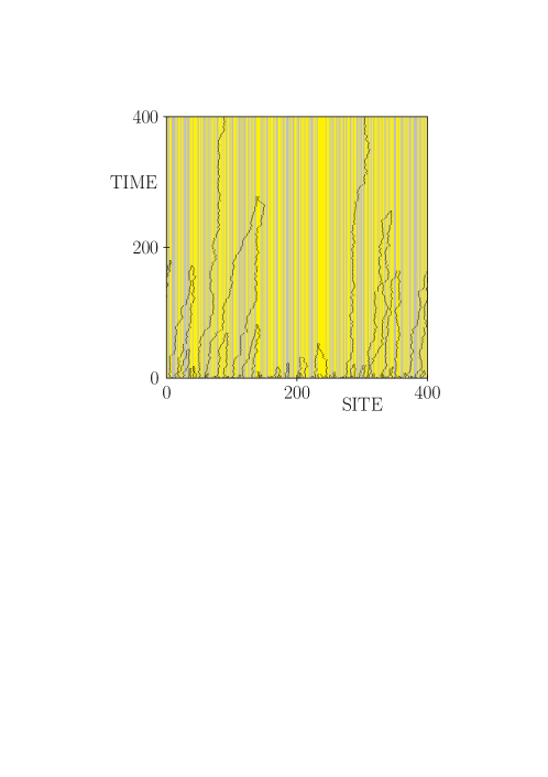
Figure 1: (Color online) Evolution snapshot, corresponding to a system with 400 sites and periodic boundary conditions, with instantaneous reaction $R_{l}=1$ and a binary distribution of diffusion biases $h_{l}-h_{l}^{\prime}\in\{0.6,\,-0.2\}$ with probability $p=0.5$ (regions in gray correspond to $h_{l}-h_{l}^{\prime}=0.6$). It can be seen that particles tend to be trapped at boundaries separating positive bias at the left from negative ones to the right.

Despite this simplicity, such modeling entails a variety of interesting aspects which play a crucial role in the subsequent analysis. These are: the nonequilibrium character of the process, formalisable in terms of a non-Hermitian quantum Hamiltonian [Robin, ]; criticality - associated with large (domain) scales, and small energies; disorder - the distributions are the source of the remarkable non universality; particle nonconservation - bringing new features to the non-universal critical phenomena through the interplay between particle and hole sectors.

This work is organized as follows. In Sec. II we present a calculation approach that exploits the quantum analogy and focuses on the spectrum gap (real part) of the associated non-Hermitian Hamiltonian. For numerical convenience the difficulties brought in by the particle nonconservation are remedied by duplicating the degrees of freedom of the original process. Sec. III outlines an analytic treatment (cf. [Dyson, ; Carlos, ]), developed from equations of motion mappings combined with renormalisation and transfer matrix techniques generalised to the non-conserving non-equilibrium nature of the system. Among the main features and procedures (briefly presented below) are: states appearing at quantised values of a complex phase obtained from phase steps for each bond and sign alternations at limiting phases; identification and aggregation of phase steps, as generalised random walks, in general biased, in the region between the limiting phases; this makes the determination of phases and their distributions a first passage problem [Redner, ] in which both the character (power law or stretched exponential) of the non-universal critical dynamics and in particular the critical exponents are determined by the effective diffusion constant and bias, inheriting their parameter-dependences (non-universality). Sec. IV implements numerically the ideas developed in Sec. II to check out the theoretical results obtained in Sec. III. The computation of finite size scaling properties of the gap yield the dynamic exponents $z$, thus providing the fundamental scaling between length and time. In addition, numerical simulations are carried out to corroborate the nonuniversal findings for $z$. Sec. V contains a summarizing discussion along with some remarks on extensions of this work.

II Fermion doubling

The common starting point for both theoretical and numerical approaches (Secs. III and IV respectively), is the representation of the evolution operator of the stochastic process, described above, as a quantum spin-$1\over 2$ non Hermitian Hamiltonian [Robin, ], which henceforth we recast as a problem of spinless fermions via a Jordan-Wigner transformation (JW) [JW, ]. Furthermore, these particles become actually free so long as the constraint

$$R_{l}=h_{l}+h^{\prime}_{l}\,,$$ (1)

is imposed for all lattice bonds [Robin, ; GS, ]. Specifically, it can be readily checked that in terms of fermion operators $C_{l},C^{{\dagger}}_{l}$, the evolution operator under these conditions reads

$$H_{C}=\sum_{l=1}^{L}\,(h_{l}+h^{\prime}_{l-1})\,C^{{\dagger}}_{l}\,C_{l}\,+\,\sum_{l=1}^{L-1}\big{(}\,R_{l}\,C_{l}\,C_{l+1}-h_{l}\,C^{{\dagger}}_{l+1}C_{l}-h^{\prime}_{l}\,C^{{\dagger}}_{l}\,C_{l+1}\,\big{)}\,+B_{C}\,,$$ (2)

($h^{\prime}_{0}\equiv h^{\prime}_{L}$). According to the parity $e^{i\pi{\cal N}_{C}}\equiv e^{i\pi\sum_{j}C^{\dagger}_{j}C_{j}}$ of the subspace considered, here

$$B_{C}=e^{i\pi{\cal N}_{C}}\left(\,h_{L}\,C^{{\dagger}}_{1}\,C_{L}+h^{\prime}_{L}C^{{\dagger}}_{L}\,C_{1}-R_{L}C_{L}\,C_{1}\,\right)\,,$$ (3)

is a boundary term stemming from the JW transformation under periodic boundary conditions (PBC).

The bilinear form imposed throughout by free fermion constraints is already very suitable for theoretical analysis (as given in Sec. III), however the pairing terms of $H_{C}$ would pose severe size restrictions in its numerical analysis, demanding the consideration of matrices growing exponentially with the length of the system. In this respect, notice that a standard Bogoliubov transformation [LSM, ] is not effective within our disordered non Hermitian context. Rather, here we follow the strategy of Ref. [MC, ] in formally related systems and proceed to double the degrees of freedom of the original problem by introducing a replica $H_{D}$ of the Hamiltonian $H_{C}$. The idea is to find a simple (i.e. disorder independent) unitary transformation so as to cancel out all non-conserving particle terms of the replicated system $H_{{}_{C+D}}=H_{C}+H_{D}$. To this end, we put forward the following fermion operators

$$f_{l} = a_{1}^{*}\,C_{l}+a_{2}\,C_{l}^{{\dagger}}+b_{1}^{*}\,D_{l}+b_{2}\,D_{l}^{{\dagger}}\,,$$

$$g_{l} = a_{3}^{*}\,C_{l}+a_{4}\,C_{l}^{{\dagger}}+b_{3}^{*}\,D+b_{4}\,D_{l}^{{\dagger}}\,,$$ (4)

with $a$’s and $b$’s coefficients such that all pairing terms are ultimately canceled in the $f-g$ representation. In fact, this can be thought of as a local Bogoliubov transformation in the real space of the double system. After some simple but lengthy algebra, we find that these coefficients should satisfy

$$a_{j}^{2}+b_{j}^{2} = 0\,,\;\;1\leq j\leq 4\,,$$

$$a_{1}\,a_{3}+b_{1}\,b_{3} = 0\,,\;\;a_{2}\,a_{4}+b_{2}\,b_{4}=0\,,$$

$$a_{2}^{*}\,a_{1}+b_{2}^{*}\,b_{1} = 0\,,\,\;\;a_{2}^{*}\,a_{3}+b_{2}^{*}\,b_{3}=0\,,$$ (5)

$$a_{1}^{*}\,a_{4}+b_{1}^{*}\,b_{4} = 0\,,\;\;a_{4}^{*}\,a_{3}+b_{4}^{*}\,b_{3}=0\,.$$

Among the various solutions we choose,

$$a_{1} = a_{2}=a_{3}=-\,a_{4}=1/2\,$$

$$b_{1} = -\,b_{2}=b_{3}=b_{4}=-\,i/2\,,$$ (6)

which leave us with a Hamiltonian of real parameters given by

$$H_{{}_{C+D}} = B_{{}_{C+D}}\,+\,\sum_{l=1}^{L-1}\,\left[\,h_{l}\left(\,f^{\dagger}_{l}\,f_{l+1}-{\rm h.c.}\,\right)+h^{\prime}_{l}\left(\,g^{\dagger}_{l+1}\,g_{l}-{\rm h.c.}\,\right)-R_{l}\left(f^{\dagger}_{l+1}\,g_{l}\,+\,{\rm h.c.}\,\right)\,\right]$$

$$+ \sum_{l=1}^{L}\,\left[\,(h_{l}+h^{\prime}_{l-1})\,\left(\,1+f_{l}^{\dagger}\,g_{l}+{\rm h.c.}\,\right)\,\right]\,.$$

As before, here $B_{{}_{C+D}}$ parallels the boundary terms referred to in Eq. (3), which in this language take the form

$$B_{{}_{C+D}} = \frac{1}{2}\left(e^{i\pi{\cal N}_{C}}+e^{i\pi{\cal N}_{D}}\right)\left[\,h_{L}\,\left(f^{\dagger}_{1}\,f_{L}-{\rm h.c.}\,\right)+h^{\prime}_{L}\,\left(\,g^{\dagger}_{L}\,g_{1}-{\rm h.c.}\,\right)+R_{L}\,\left(f^{\dagger}_{1}\,g_{L}+{\rm h.c.}\,\right)\,\right]$$ (8)

$$+ \frac{1}{2}\left(e^{i\pi{\cal N}_{C}}-e^{i\pi{\cal N}_{D}}\right)\left[\,h_{L}\,\left(f^{\dagger}_{1}\,f^{\dagger}_{L}-{\rm h.c.}\,\right)+h^{\prime}_{L}\,\left(\,g^{\dagger}_{1}\,g^{\dagger}_{L}-{\rm h.c.}\,\right)+R_{L}\,\left(g_{L}^{\dagger}\,f^{\dagger}_{1}+{\rm h.c.}\,\right)\,\right]\,.$$

Therefore, the number of $f$ and $g$ particles is conserved as all pairing terms actually cancel out, provided we restrict attention to subspaces having $(-1)^{{\cal N}_{C}}=(-1)^{{\cal N}_{D}}$.

In passing, it is instructive to check how the exact solution of the homogeneous situation is recovered by Fourier transforming the $f_{l}$ and $g_{l}$ operators respectively to a set of new wave fermions $f_{q},\,g_{q}$. To account for the parity conserving terms implicated in $B_{{}_{C+D}}$, the $q$-momenta must be those of the set $Q^{+}=\left\{\pm\pi/L,\,\pm 3\pi/L,\,\cdots\,,\pm(L-1)\pi/L\right\}$ for the even subspace, while for the odd one the $q$’s should belong to $Q^{-}=\left\{\pm 2\pi/L,\,\pm 4\pi/L,\,\cdots\,,\pm(L-2)\pi/L,0,\pi\right\}$, say for $L$ even. After straightforward algebraic steps, it is readily found that the ordered Hamiltonian $H_{o}$ [ i.e. $R_{l}=R,\,h_{l}=h,$ and $h^{\prime}_{l}=h^{\prime}\,\;\forall\,l\,$ in Eq. (II) ] reduces to

$$H_{o}=R\,L+\sum_{q}\left(\begin{array}[]{ccc}f_{q}^{\dagger}&,&g_{q}^{\dagger}\end{array}\right)\left[\begin{array}[]{cc}i\,2h\sin q&R\,(1-e^{-iq})\\ \\ R\,(1-e^{iq})&-\,i\,2h^{\prime}\sin q\end{array}\right]\,\left(\begin{array}[]{c}f_{q}\\ \\ g_{q}\end{array}\right)\,.$$ (9)

Using a simple non unitary $2\times 2$ similarity transformation to new $F_{q}^{\pm},G_{q}^{\pm}$ fermion like operators [algebra, ], the double system is finally diagonalized as

$$H_{o} = R\,L+\sum_{q\in Q^{\pm}}\Lambda_{q}\,F^{+}_{q}\,F^{-}_{q}\,-\,\sum_{q\in Q^{\pm}}\Lambda_{-q}\,G^{+}_{q}\,G^{-}_{q}\,,$$

$$\Lambda_{q} = R\,(1-\cos q)+i\,(h-h^{\prime})\sin q\,.$$ (10)

Thus, in doubling the degrees of freedom the $\Lambda_{q}$ excitations of the original problem are restored [GS, ], but now they appear forked in two symmetrical branches $\Lambda_{q},-\Lambda_{-q}$ around a Fock vacuum with ”energy” $R\,L$ rather than with vanishing value, as it would correspond to the stationary state of the original stochastic $H_{C}$. Hence, in general the doubling transformation (4) should not be regarded as a similarity one, although it preserves all the anticommutation relations which is enough to maintain the spacing of eigenlevels, and in particular the spectrum gap. In the homogeneous case, this scales as $1/L^{2}$, so the usual dynamic exponent $z=2$ is restituted.

For the more interesting disordered situation, if we think of $\{f_{1},g_{1},\,\cdots\,,f_{L},g_{L}\}$ as the $2L$ single particle states of the replicated Hamiltonian $H_{{}_{C+D}}$, then the single excitations of Eq. (II) can be obtained by diagonalizing the real non symmetric five-diagonal matrix (with boundary conditions)

$$M_{\pm}=\left[\begin{array}[]{cccccccc}{\cal R}&h_{1}+h^{\prime}_{L}&h_{1}&0&\cdots&0&\pm h_{L}&\pm R_{L}\\ \\ h_{1}+h^{\prime}_{L}&{\cal R}&-R_{1}&-h^{\prime}_{1}&0&\cdots&0&\mp h^{\prime}_{L}\\ \\ -h_{1}&-R_{1}&{\cal R}&h_{2}+h^{\prime}_{1}&h_{2}&0&\cdots&0\\ 0&h^{\prime}_{1}&h_{2}+h^{\prime}_{1}&{\cal R}&-R_{2}&-h^{\prime}_{2}&0&\vdots\\ &\vdots&&&\hskip-42.67912pt\ddots&&\vdots&\\ \vdots&0&-h_{L-2}&-R_{L-2}&{\cal R}&h_{L-1}+h^{\prime}_{L-2}&h_{L-1}&0\\ \\ 0&\cdots&0&h^{\prime}_{L-2}&h_{L-1}+h^{\prime}_{L-2}&{\cal R}&-R_{L-1}&-h^{\prime}_{L-1}\\ \\ \mp h_{L}&0&\cdots&0&-h_{L-1}&-R_{L-1}&{\cal R}&h_{L}+h^{\prime}_{L-1}\\ \\ \pm R_{L}&\pm h^{\prime}_{L}&0&\cdots&0&h^{\prime}_{L-1}&h_{L}+h^{\prime}_{L-1}&{\cal R}\end{array}\right]\,,$$

where ${\cal R}=\sum_{j}R_{j}$. The numerical diagonalization of $M_{\pm}$ [NR, ] reveals the emergence, as before, of two symmetrical branches $\{{\cal R}+\Lambda\},\,\{{\cal R}-\Lambda\}$ of single excitations around a ground state energy ${\cal R}$. Denoting by $\Lambda^{\pm}_{0}$ the lowest level excitation in either subspace ( ${\rm Re}\;\Lambda_{0}^{\pm}={\rm min\;\{Re}\;\Lambda^{\pm}\}\,)$, the spectrum gap $g$ of the original evolution operator (2) with an initially even (odd) number of reacting-diffusing particles, is finally obtained as $g=2\,{\rm Re}\;\Lambda^{+}_{0},$ with a doubly degenerate $\Lambda^{+}_{0}$ ($g={\rm Re}\;\Lambda^{-}_{0},\;$ with $\Lambda^{-}_{0}$ being non degenerate).

We will recapitulate these ideas in the numerical diagonalizations of Sec. IV so as to account for the theoretical findings of the next section.

III Phase steps as random walks

In what follows we reconsider the non-conserving fermion Hamiltonian (2), but without fermion doubling. One of the eigenvalue equations associated to that operator involves only ”hole” state amplitudes $a_{l}$ at each site $l$. These provide an inhomogeneous term in the other equation, for the ”particle” states $a^{+}_{l}$. Using two-component vectors, the eigenvalue equation involves $2\times 2$ matrix coefficients which depend on the excitation ”energy” $\Lambda$, and on bond-dependent biased hopping and bond-independent pair annihilation rates $h_{l},h^{\prime}_{l},R_{l}$, constrained as in Eq. (1), to keep the free-fermion character. The product of the associated $4\times 4$ transfer matrices, $\prod_{l=1}^{L}T_{l}$, provides the spectrum through its trace, or appropriate matrix elements (depending on boundary conditions), effectively corresponding to quantisation of an aggregated phase. One $2\times 2$ part of $T_{l}$ is the transfer matrix $t_{l}$ for the self-contained subspace (”hole sector”) provided by the states $a_{l}$.

From the coupled eigenvalue equations one may equivalently proceed via the corresponding $4\times 4$ transfer matrix $T_{l}$, or via renormalisation using a decimation method, or by mapping ratios of successive amplitudes. Here we mainly employ the last approach. The transfer matrix and decimation approaches are very instructive, in clarifying respectively the role of accumulating complex phases (which provide the spectrum) and the renormalization of quenched probability distributions of such aggregated variables, but in what follows it is sufficient and convenient to begin with the transfer matrix and then move over to the mapping approach.

For orientation and to obtain certain characteristic parameters it is useful to separate the rates (and consequently the transfer matrix itself) into reference uniform, $l$-independent, ”effective medium” parts ($h,h^{\prime}=R-h$, indicated by the absence of a site label), together with the further random part involving a disorder strength $\delta$, and (binary) random variables $\zeta_{l}$ at each bond. Then $T_{l}$ becomes $T_{l}\equiv T+\hat{\Delta}_{l}$. For any finite size $L$, it is possible to start from $T$ and build in the disorder terms $\hat{\Delta}_{l}$ completely. For that, it is convenient to work in the representation diagonalising $T$. Two ($i=1,2$ say) of the four labels on its eigenvalues $\lambda_{i}$ relate to the ”hole” sector part $t_{l}$ of the transfer matrix. The ”particle” sector ($i=3,4$) couples to the other sector through the inhomogeneous term referred to above. The eigenvalues are conveniently parametrised as $\lambda_{1,2}=\sqrt{h^{\prime}/h}\,\exp(\pm iq)$, where $q$ satisfies $\Lambda=1-2\sqrt{h^{\prime}h}\,\cos q$, with a similar form (with $\Lambda$ changed sign) for $\lambda_{3},\lambda_{4}$.

The formal expansion in powers of $\hat{\Delta}_{l}$ gives

$${\rm Tr}\;\prod_{l=1}^{L}T_{l}=\sum_{n=0}^{L}(A_{n}+B_{n}),,$$ (11)

where $A_{n}$ and $B_{n}$ come respectively from the $i=1,2$, and $i=3,4$ terms in the trace, and each involves sums over $n$ disorder variables. For example,

$$A_{n}=(4\,\delta)^{n}\,\left(h^{\prime}/h\right)^{L\over 2}\underbrace{\sum_{m_{1}\geq 1}\,\sum_{m_{2}\geq 1}...\sum_{m_{n}\geq 1}}_{\sum_{i=1}^{n}\,m_{i}=L}\,\zeta_{{}_{m_{1}}}\,\zeta_{{}_{m_{1}+m_{2}}}\,...\,\,\zeta_{{}_{m1+...+m_{n}}}\,\prod_{i=1}^{n}\eta\,(m_{i}q)\,,$$ (12)

where $\eta(mq)$ is a periodic function involving separations $m_{i}$ of the participating disorder sites and connected with competing aspects of the wavelength and scales set by the local disorder and bias. $B_{n}$ involves a part similar to $A_{n}$ and a second more complex part generated by the inhomogeneous terms.

It is instructive to consider the approximation to the multiple sum in Eq. (12) coming from taking all $m_{i}$ as large. In this case the $q$-dependence in the functions $\eta(m_{i}q)$ goes into an overall exponential factor, and the product of these factors comes out of the multiple sum as a complex phase factor $\exp(\pm i\,Lq)$ also accompanied by further $q$-independent factors. The summand is then just the product of disorder variables $\zeta_{...}$ and the sum can be shown to be the coefficient of $x^{n}$ in the generating function $\prod_{l=1}^{L}(1+x\zeta_{l})$. Taken together with the other factors that leads to $\sum_{n=0}^{L}A_{n}$ being the exponential of an aggregated complex phase with real and imaginary parts $\sum_{l=1}^{L}\phi_{l}$ and $i\,L{\rm Re}\,(q)$, where

$$\phi_{l}=\ln\,(h^{\prime}_{l}/h_{l})\,.$$ (13)

For binary random rates the sum of $\phi_{l}$ is like a random walk. The case of most interest is when the two possibilities have different signs (orientations) for the bias $h_{l}-h^{\prime}_{l}$ , so steps occur in both directions. The same phase step (though aggregated in various different ways) occurs in the parts of the corresponding approximation for $\sum_{n=0}^{L}B_{n}$ coming from the inhomogeneous terms; the remaining ”homogeneous part” has negligible phase step.

However, in the approximation the location of states then becomes the same as for the pure system - coming just from $i\,L{\rm Re}\,(q)$ since the disorder dependence of the phase is now confined to the real function $\phi_{l}$. So it will be necessary to generalise the result obtained by taking characteristic $m$’s as large, by retaining the registration between local disorder and aggregating phase which is provided by the functions $\eta(m_{i}q)$. This is most easily done by working with the fully-disordered transfer matrix (or directly from the original equations of motion). That gives, as follows, information on characteristic scales, domain structures, phase accumulations, and the region of validity of the approximation just discussed. For the phases from $\sum_{n=0}^{L}A_{n}$ (the simplest illustration) only the $2\times 2$ subpart $t_{l}$ corresponding to the hole sector of the (fully-disordered) transfer matrix $T_{l}$ is needed.

The crucial aggregating phase variable is $\ln\,x_{l}$, where $x_{l}=(a_{l-1}/a_{l})$ is the ratio of complex amplitudes $a_{l}$ on successive sites. These $x_{l}$ ratios satisfy

$$\left(\begin{array}[]{c}x_{l+1}^{-1}\\ 1\end{array}\right)=t_{l}\left(\begin{array}[]{c}1\\ x_{l}\end{array}\right)\,.$$ (14)

From this it follows that $x_{l}=g_{l}(h^{\prime}_{l-1}/h_{l-1})$, where $g_{l}$ is such that $z_{l}\equiv(1-g_{l})^{-1}$ satisfies

$$z_{l+1}=[(h_{l}+\Lambda)z_{l}+h^{\prime}_{l-1}]/[\Lambda z_{l}+h^{\prime}_{l-1}]\,.$$ (15)

From this (Mobius) map, and its first iteration yielding $z_{l+2}$ , it can readily be seen that when

$$z^{<}_{l}\equiv\frac{h^{\prime}_{l-1}}{h_{l}}\,[\,1+{\cal O}(\Lambda)\,]\ll|z_{l}|\ll\frac{h^{\prime}_{l-1}}{\Lambda}\equiv z^{>}_{l}\,,$$ (16)

(needing $\Lambda$ small) the variable $\chi_{l}\equiv\ln\,z_{l}$ ”walks” according to $\chi_{l+1}\sim\chi_{l}+\ln\,(h_{l}/h^{\prime}_{l-1})$ while the complex phase step in $a_{l}$ is $\ln\,x_{l}=\ln\,[g_{l}(h^{\prime}_{l-1}/h_{l-1})]\sim\ln\,(h^{\prime}_{l-1}/h_{l-1})=\phi_{l-1}$, as was found in Eq. (13) using the approximation on $\sum_{n=0}^{L}A_{n}$. Near $z_{l}=z^{>}$ (or $z^{<}$), the mapped $z$ goes to $\infty$ (or 0, then 1, giving a vanishing amplitude) and changes sign. This procedure thus provides the region (16) of validity of the approximation on $\sum_{n=0}^{L}A_{n}$, and generalises it: the behaviour at $z=z^{<},z^{>}$ is the proper consequence of the functions $\eta(m_{i}q)$, replacing the sign changes given by $\exp(\pm i\,Lq)$ in the approximate result.

In the corresponding discussion for the structure and phases in $\sum_{n=0}^{L}B_{n}$ (coming from ”particle” states, with complex amplitudes $a^{+}_{l}$), linearity allows a separation into two parts: (i) without, and (ii) with, the mixing to the states in the ”hole” subspace just treated. The discussion for the first part ((i)) is similar to that just given, and leads to a walk step $\ln\,(a^{+}_{l-1}/a^{+}_{l})\equiv\ln\,c^{+}_{l}$ with $c^{+}_{l}$ close to 1 if $y_{l}\equiv(1-c^{+}_{l})^{-1}$ satisfies a condition like (16), with the same limits $z^{<},\,z^{>}$ to leading order in $\Lambda$. For small $\Lambda$, $\varphi_{l}\equiv\ln\,y_{l}$ walks with the same step as $\chi_{l}=\ln\,z_{l}$, and has the same behaviour at the limiting values. For part (ii), the inhomogeneous term coming from the mixing to the states in the other subspace leads to the occurrence again of $z_{l}$ and $x_{l}=(a_{l-1}/a_{l})$, in terms of which, for $z^{<}\ll z_{l}\ll z^{>}$ (so $\Lambda$ is small and $x_{l}\sim(h^{\prime}_{l-1}/h_{l-1})$) , the amplitude ratio is $a^{+}_{l}/a^{+}_{0}=1+\sum_{j=0}^{l-1}(\Gamma_{l}/h_{l})$ where

$$\Gamma_{l}\equiv h_{l}(a^{+}_{l+1}-a^{+}_{l})=a_{0}\prod_{j=0}^{l+1}\gamma_{l}^{-1}+A_{0}\prod_{j=0}^{l}\gamma_{l},\;l\geq 1\,,$$ (17)

with $\gamma_{l}=h^{\prime}_{l}/h_{l}$, and $A_{0}=\Gamma_{0}-a_{0}/x_{1}$.

The combination of these results from (i),(ii) gives the essence of the complicated result for the approximated $\sum_{n=0}^{L}B_{n}$, together with its validity criterion, and again generalises it as necessary to obtain and quantize the imaginary part of the phase, to enumerate the states: the limiting boundary phase conditions provide the sign reversals in amplitude and correspond to (reflecting and absorbing) boundary conditions on the walks described above.

Since the walk steps of $\chi_{l}$ and $\varphi_{l}$ contain disorder we need the probability distributions $P(\chi_{l})$ and $P(\varphi_{l})$, which are the same for small $\Lambda$. The distributions depend on the boundary conditions, and are most easily treated in a continuum (diffusion) picture. There, $l$ plays the role of time, and the accumulating $\chi_{l}$ or $\varphi_{l}$ plays the role of spatial coordinate. From the walk steps described above, within the limits set by Eq. (16), the distributions satisfy a standard biased diffusion equation having diffusion constant $D$ and bias $b$ given by

$$D = \frac{1}{2}\,{\rm var\;\ln\,}\,(h_{l}/h^{\prime}_{l})\,\,,$$

$$b = \langle\,\ln\,\,h_{l}\,\rangle-\langle\,\ln\,\,h^{\prime}_{l}\,\rangle\,.$$ (18)

The boundary conditions take the biased problem to first-passage form [Redner, ] in which many reflections of the walk occur before absorption is reached, with probability exponentially small in the traversal ”length”. The boundary conditions set the limits to the excursion (of the walk), making the traversal ”length”

$$\ln\,z^{>}-\ln\,z^{<}=\ln\,(\Lambda_{0}/\Lambda),\;\Lambda_{0}\sim h\,,$$ (19)

(long, as required for the continuum picture, in the critical regime of small $\Lambda$). Consequently, the first passage ”time” scale ${\cal L}\sim L$, is proportional to $\exp[(|b|/D)\ln\,(\Lambda_{0}/\Lambda)]$ , which can be written in the scaling form $\Lambda^{-1/z}$ with dynamic exponent

$$z=D\,/|\,b\,|.$$ (20)

In the opposite case of large bias, applying for nearly homogeneous systems, the effects of $({\rm Re}\;\Lambda)^{1/2}$ dominate making $z$ close to 2.

From the exponential distribution $P(\chi)\propto\exp[-\,(\,|\,b\,|/D)\,\chi]$ for $\chi$ (and similarly $\varphi$), the energy distribution is appreciable only at $\chi=\ln\,z^{<}(\Lambda)$. That gives the exponential energy distribution

$$P(\Lambda)\propto\exp[-\,\Lambda\,|\,b\,|\,h^{\prime}/(D\,h)\,]\,,\;\;{\rm for}\;\;\Lambda\gtrsim{\cal L}^{-z}\,.$$ (21)

It can be seen that the dynamic exponent $z$ is non-universal because the distribution of the random rates allows both signs of the walk steps and is (in general) parameter-dependent. In particular, $z$ can diverge if the bias $b$ becomes zero (for example, at a critical concentration $p_{c}$ in the binary case studied below in Sec. IV). Then a stretched exponential scaling form emerges as follows. For the unbiased case the first passage problem has standard $\chi^{2}\propto D\cal L$ relation between the ”length” and ”time” scales. That makes $[\ln\,(\Lambda_{0}/\Lambda)]^{2}\propto D\cal L$, consequently

$$\Lambda/\Lambda_{0}\sim\exp\left(\,-c\,{\cal L}^{\beta}\right)\,,$$ (22)

with $\beta=1/2$ and $c=c_{0}D^{1/2}$, with $c_{0}$ a numerical constant of order one. In this case (where the bias vanishes) the Gaussian distribution for the aggregated phase produces a gap distribution with exponential tails. Consequently, for $b\rightarrow 0$ , the ratio of rms gap to mean gap diverges.

IV Numerical results

To check out the above expectations, we now investigate numerically the finite size behavior of the gap of the original evolution operator (2) when averaged over independent disorder realizations. To this end, we diagonalize the $M_{\pm}$ matrices referred to in Eq. (II) given in Sec. II, and whose dimensions just grow linearly with the system size. For concreteness and comparison with the analytical results of Sec. III, let us consider a binary distribution of bonds with parameters $B_{1,2}=\{R_{1,2}\,,\,h_{1,2}\}$, and probability $P(B)=p\,\delta_{B,B_{1}}+(1-p)\,\delta_{B,B_{2}}$. For a given concentration $p$, we averaged spectra typically over 6000 samples of chains with lengths $50\leq L\leq 1000$. For most $p$ the resulting average gaps scale as $\langle g\rangle\propto L^{-z}$ irrespective of parity, and eventually with non-universal dynamic exponents $z=z(p)$, as it was established by Eq. (20) in Sec. III. This situation is exhibited in Fig. 2, where we show a characteristic case of instantaneous reactions under orientation changes in diffusion biases $h-h^{\prime}$, these latter satisfying the free fermion constraint (1) imposed throughout.

Figure 2: Average spectrum gap $\langle g\rangle$ for a binary distribution of biases $\{0.6,\,-\,0.2\}$, and instantaneous reactions ($R_{1,2}\equiv 1$). The concentration varies from top to bottom as $p=$ 0.5, 0.75, 0.3, 0.25. Dynamic exponents $z$ are read off from the slopes of the fitting lines. For displaying purposes, data have been shifted slightly upwards with respect to $p=0.25$. The inset shows the stretched exponential scaling expected at $p_{c}\sim 0.2263$ under free boundaries.

On approaching the critical regime defined by the unbiased diffusion equation referred to earlier on in Sec. III, finite size effects become progressively pronounced until at a critical concentration $p_{c}$, given by

$$p_{c}=\left[\,1-\frac{\ln\left(\frac{1-h_{1}}{h1}\right)}{\ln\left(\frac{1-h_{2}}{h2}\right)}\,\right]^{-1},\;\;h_{1}\,^{<}{}_{>}\;\frac{1}{2}\;^{<}_{>}\,h_{2}\,,$$ (23)

[ i.e. $b=0$, in Eq. (18) ], the length scaling of the gap crosses over to the stretched exponential form conjectured above in Eq. (22). This is corroborated in the inset of Fig. 2 which

Figure 3: Non-universal dynamic exponents of the binary distribution of Fig. 2. Filled circles near $p_{c}$ stand for lower bounds of $z$. In the inset these latter support the divergence trend of the analytical results close to criticality [Eq. (20) in dashed curves ].

for large sizes (and open boundaries [PBC, ] ), supports the universal stretching factor $\beta=1/2$ involved in (22). Thus, in nearing $p_{c}$ the stochastic dynamics slows down dramatically which, in line with the approach of the preceding section, is reflected in the abrupt increase of dynamic exponents observed in Fig. 3. As we have seen in Eq. (20), for $p\to p_{c}$ these latter can be arbitrarily large in the thermodynamic limit, but in practice they are ultimately cutoff by our available system sizes. In this regard, notice that the trend of slopes obtained near the critical region (e.g. lowermost curve of Fig. 2), constitutes a numerical lower bound for these exponents (filled symbols of Fig. 3).

Figure 4: Distributions of gaps $(g)$ for binary disorder over 500 sites. In (a) the parameter rates are taken as in Fig. 2; the main panel shows (part of) the case $p=p_{c}$ ($\sigma/\langle g\rangle\sim 2$), whereas the inset displays a characteristic non-critical situation ($p=0.5,\,\sigma/\langle g\rangle\sim 0.6$). Both results have exponential tails (in bold lines). (b) shows a typical well defined bias case $(\{0.6,0.2\},\,p=0.5)$, exhibiting instead a narrow distribution closely following a Gaussian (in dashed line, $\sigma/\langle g\rangle\sim 0.02$). As is shown in the inset, here dynamic exponents are diffusive.

Also, in agreement with the theoretical analysis, it is seen that the distribution of spectral gaps becomes broadest at $p_{c}$ (maximum variance $\sigma$). This is illustrated in Fig. 4a, after binning gaps in 800 intervals over 60.000 disorder realizations. By contrast, chains with non-fluctuating bias orientations have rather narrow gap distributions, and typically diffusive dynamic exponents ($z=2)$, regardless of the value of $p$. This characteristic scenario already anticipated in Sec. III, is exhibited in Fig. 4b.

Simulations.– To allow for an independent examination of nonuniversal aspects, we also carried out numerical simulations in periodic chains of 200, 400 and 800 sites (without duplication). Averages of particle densities were taken over $10^{3}$ histories of $10^{3}$ samples with binary disorder. Starting from homogeneous densities $\rho$, our results in Fig. 5 clearly indicate an asymptotic decay of the form $\langle\rho_{L}(t)\,\rangle\propto e^{-t/\tau_{L}}$ with a relaxation time $\tau_{L}\propto L^{z}$. As expected, the slope collapse follows closely the non-universal dynamic exponent already identified by direct diagonalization ($z\sim 1.64$, in Fig. 2). In turn, the best scaling behavior for well oriented biases is obtained with standard diffusive exponents, which is also in agreement with our previous numerical results (inset of Fig. 4b).

Figure 5: Density decay for the distribution of Fig. 2 exhibiting a non-universal dynamic exponent at $p=0.5$. The inset shows the case of a well defined sign of binary biases $\{0.6,\,0.2\}$ (as in Fig. 4b), displaying instead a typical diffusive exponent. Squares denote data for $L=800$, circles 400, and triangles 200. To compare slopes, the data of these latter two sizes were shifted downwards.

Finally, it is interesting to comment on the regime $t\ll L^{z}$. This latter is addressed in Fig. 6 where the density decay below, at, and above $p_{c}$ is exhibited for much larger systems. After averaging 20 samples over 100 histories each, it is observed that in all cases there is an early stage showing the typical $t^{-1/2}$ decay. However, at $p=p_{c}$ ($p>p_{c}$), an incipient crossover to a slower (faster) decay clearly emerges (cf. [Gunter, ; Krapivsky, ]). It would take further evolution decades to estimate the actual form of such regimes, although their nonuniversal characters are already in line with our findings for $z(p)$. The situation for $p<p_{c}$ remains unclear as the existence of a very slow crossover can not be ruled out.

Figure 6: Density decay for the binary distribution considered above, using $L=10^{4}$ and different concentrations. From top to bottom these vary as $p_{c}\sim 0.2263$ (circles), $0.15$ (triangles) , and $0.5$ (squares). For comparisons of large times trends, the data of the latter two concentrations were shifted downwards. Solid lines are fitted with slopes -1/2.

V Conclusions

To summarise, after identifying phase steps, and limiting phases and their relationship to generalised biased random walks, in Sec. III we have outlined how the character (power law or stretched exponential) of the non-universal critical dynamics and in particular the critical exponents and their non-universality are determined by the associated diffusion constant and bias (in the case where the fundamental phase step can have either sign).

Among the specific results given above are: in the general biased case the dynamic exponent $z$ is $D/|b|$ and associated distributions of the energy gap are exponential. For vanishing bias $z$ diverges and the usual critical power law behaviour is replaced by a stretched exponential form, possibly signaling the emergence of a glassy dynamic, while the ratio of rms gap to mean gap diverges. All those findings were corroborated numerically using the doubling fermion approach given in Sec. II and Monte Carlo simulations of Sec. IV.

Concerning occurrence of both positive and negative phase steps, that is connected, in a given configuration of randomness, to a succession of domains of alternating bias, whose boundary sites alternate between being traps or repellers for particles. That causes some particles to wander ineffectively for long times before finding a partner for pair annihilation (see Fig. 1), leading to large or divergent dynamic exponents (see Figs. 2 and 3).

Among many important things not covered are: the full parameter-dependence of dynamic exponent $z$ from pure value to divergence where the bias vanishes (e.g. in the case of the binary distribution of rates, with concentration parameter p, where $z(p)$ is not monotonic for $p$ in $[0\,,\,p_{c}]$ or in $[p_{c}\,,\,1]$); the effect of open boundaries versus PBC (can be very significant in driven non-equilibrium systems) - particularly here regarding the stretching exponent for zero bias - needs further investigation.

References

- (1) G. Ódor, Rev. Mod. Phys. 76, 663 (2004).
- (2) F. Iglói and C. Monthus, Phys. Rep. 412, 277 (2005).
- (3) A. O. Golosov, Comm. Math. Phys. 92, 491 (1984).
- (4) P. Le Doussal and C. Monthus, Phys. Rev. E 60, 1212 (1999).
- (5) G. M. Schütz and K. Mussawisade, Phys. Rev. E 57, 2563 (1998).
- (6) P. L. Krapivsky, E. Ben-Naim, and S. Redner, Phys. Rev. E 50, 2474 (1994).
- (7) N. Kuroda et al., Phys. Rev. B 61, 11217 (2000); Phys. Rev. Lett. 79, 2510 (1997); Phys. Rev. B 59, 12973 (1999).
- (8) R. B. Stinchcombe, Adv. Phys. 50, 431 (2001); G. M. Schütz, in Phase Transitions and Critical Phenomena, C. Domb and J. L. Lebowitz eds. (Academic, London 2001).
- (9) F. J. Dyson, Phys. Rev. 92, 1331 (1953); H. Schmidt, Phys. Rev. 105, 425 (1957); T. P. Eggarter and R. Riedinger, Phys. Rev. B 18, 569 (1978).
- (10) F. Iglói and I. A. Kovács, Phys. Rev. B 77, 144203 (2008); C. A. Lamas, D. C. Cabra, M. D. Grynberg, and G. L. Rossini, Phys. Rev. B 74, 224435 (2006).
- (11) S. Redner, A Guide to First-Passage Processes, (Cambridge University Press, 2001).
- (12) P. Jordan and E. Wigner, Z. Phys. 47, 631 (1928).
- (13) M. D. Grynberg and R. B. Stinchcombe, Phys. Rev. Lett. 76, 851 (1996); Phys. Rev. Lett. 74, 1242 (1995); Phys. Rev. E 52, 6013 (1995).
- (14) See e.g. E. Lieb, T. Schultz, and D. Mattis, Ann. Phys. (NY) 16, 407 (1961).
- (15) F. Merz and J. T. Chalker, Phys. Rev. B 65, 054425 (2002).
- (16) Here, , but satisfy the elementary excitation algebra: .
- (17) Consult for instance, W.H. Press, S.A. Teukolsky, W.T. Vetterling and B.P. Flannery, Numerical Recipes, 2nd ed. (Cambridge University Press, 1992); see Chapter 11.
- (18) Under PBC however, our diagonalizations suggest instead a stretching factor .