Superfocusing by Nano-Shells

Abstract

Recently Merlin and co-workers demonstrated, both theoretically and in the microwave range experimentally, subwavelength focusing of evanescent waves by patterned plates. The present paper extends these ideas and the design procedure to scatterers of arbitrary shapes and to the optical range of wavelengths. The analytical study is supported by numerical results. The most intriguing feature of the proposed design is that, in the framework of classical electrodynamics of continuous media, focusing can in principle be arbitrarily sharp, subject to the constraints of fabrication.

OCIS numbers: 310.6628, 160.4236, 350.4238, 240.6680, 250.5403, 050.1970.

Subwavelength focusing that circumvents the usual diffraction limit in optics has been a very active area of research, with a multitude of approaches explored in the literature: negative-index lenses and guides, plasmonic particles and cascades, superoscillations, time-reversal techniques and others (Zheludev-What-diff-limit-08 –Dai08 and references therein). Recently the Merlin and Grbic groups Merlin-Radiationless-interference-07 ; Grbic-Near-field-plates-08 (see also Helseth-almost-perfect-lens-08 ) showed, both theoretically and in the microwave range experimentally, that patterned (grating-like) plates produce subwavelength focusing of evanescent waves if the pattern contains significantly different spatial scales of variation. Conceptually, these patterns are related to surface profiles of near-field optical holography Bozhevolnyi-near-field-holography96 .

This Letter shows that the ideas of near-field focusing can be extended to patterned nano-shells and, further, to scatterers of arbitrary shape. The most intriguing feature is “superfocusing” – i.e. focusing that can in principle be arbitrarily sharp and strong, subject to the constraints of fabrication and availability of materials with desired values of the dielectric permittivity $\epsilon$. (It is also tacitly assumed that the size of the system is sufficiently large for electrodynamics of continuous media to be applicable; see e.g. Dai08 and references therein.)

Let us suppose that an incident plane wave with a frequency $\omega$ impinges on a scatterer coated with a plasmonic and/or dielectric layer. In general, the shape of the scatterer may vary; more importantly, the thickness and dielectric permittivity of the coating may be chosen judiciously, with the ultimate goal of nano-focusing the wave at a given spot. In practical applications, the role of the scatterer can be played e.g. by the apex of an optical tip, the active part of an optical sensor or by a nano-antenna.

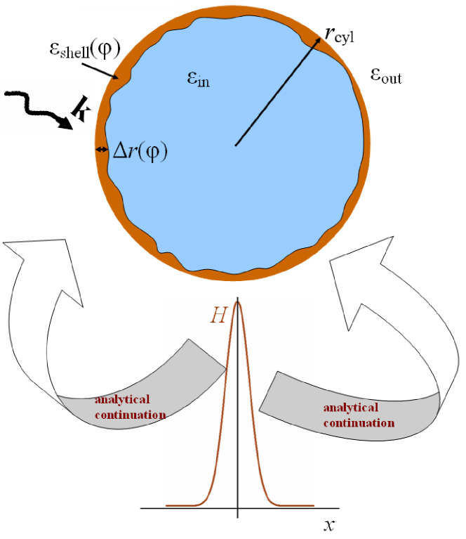
Figure 1: A thin shell (coating) can be capable of focusing light to an arbitrarily narrow spot if the angular variation of its dielectric function and/or thickness are judiciously chosen. See text for further details.

Even though the ideas are general and could be applied in 3D electrodynamic analysis and design, let us consider for maximum simplicity the 2D case of a cylindrical scatterer (particle) of radius $r_{\mathrm{cyl}}$ (Fig. 1). The usual complex phasor convention with the $\exp(-\mathrm{i}\omega t)$ factor is adopted.

Several ways of formulating this electromagnetic field problem are available. First, one needs to distinguish full electrodynamic analysis vs. quasi-static (QS) approximations valid for dimensions much smaller than the wavelength. The QS treatment has limitations, as it does not account for wave effects and short-range surface plasmon modes Valle-Sondergaard-Bozhevolnyi-SPP-resonators08 . However, to fix ideas and for the sake of algebraic simplicity this Letter adopts the QS approximation. Full wave analysis is analogous but involves Bessel/Hankel functions and their derivatives instead of polynomials in $r$ (see expressions below).

Second, the electrodynamic problem may be formulated in terms of the electric or magnetic field (convenient for $s$- and $p$-polarizations, respectively). Alternatively, two dual formulations are also available under the QS approximation: via the electric scalar potential and via the stream function $\mathbf{\Psi}$, $\nabla\times\mathbf{\Psi}=\epsilon\mathbf{E}$ ; see Shvets-Urzhumov-04 ; Mayergoyz05 for some interesting implications of this duality.

Let us endeavor to achieve sharp focusing with respect to the polar angle $\phi$ at a certain radius $r_{f}>r_{\mathrm{cyl}}$. For $p$-polarization (the two-component electric field in the cross-sectional plane and the one-component magnetic field $H$ directed along the axis of the particle), let

$$H_{\mathrm{out}}(r_{f},\phi)~{}=~{}H_{f}g(\phi-\phi_{f})$$ (1)

where $H_{\mathrm{out}}$ is the magnetic field outside the shell, $H_{f}$ is some amplitude at the focus, $\phi_{f}$ is a given angle and $g(\phi)$ is a desired distribution of the field. For example, choosing $g(\phi)$ or, alternatively, $g^{\prime}(\phi)$ as a sharp Gaussian peak will result in the corresponding peak in the magnetic field or the radial component of the electric field, respectively.

This local behavior of the field can be extended, by analytical continuation, to the whole region outside the scattering shell. One way of doing so is by expanding the field into cylindrical harmonics whose coefficients are found from the Fourier transform of $g$. This analytical continuation will then determine the field distribution on the surface of the particle, and one needs to find the parameters of the coating that would produce such a surface distribution.

More specifically, in the QS limit the field inside the shell can be expanded into cylindrical harmonics:

$$H_{\mathrm{in}}(r,\phi)~{}=~{}\sum_{n=-\infty}^{\infty}a_{n}r^{|n|}\exp(\mathrm{i}n\phi),~{}~{}r\leq r_{\mathrm{cyl}}$$ (2)

where $a_{n}$ are some coefficients. Outside of the cylinder ($r>r_{\mathrm{cyl}}$) the magnetic field can be represented as the sum of the incident field and the scattered field:

$$H_{\mathrm{out}}~{}=~{}H_{\mathrm{INC}}\,+\,H_{\mathrm{s}}$$ (3)

The incident field under the QS approximation is linear with respect to $r$:

$$H_{\mathrm{INC}}~{}=~{}H_{0}\,+\,h_{0}r\cos(\phi-\phi_{0})$$ (4)

where $h_{0}$ is a coefficient. The constant $H_{0}$ does not affect the results and is for simplicity set to zero in the remainder. The scattered field is

$$H_{\mathrm{s}}(r,\phi)~{}=~{}\sum_{n=-\infty}^{\infty}c_{n}r^{-|n|}\exp(\mathrm{i}n\phi)$$ (5)

where $c_{n}$ are coefficients to be determined.

The boundary conditions across the coating are as follows. If the coating is nonmagnetic and thin, the magnetic flux passing through it can be neglected and consequently the tangential component $E_{\phi}$ of the electric field is assumed to be continuous across the coating:

$$E_{\phi,\mathrm{out}}~{}=~{}E_{\phi,\mathrm{in}}$$ (6)

Substituting

$$E_{\phi}~{}=~{}\frac{1}{\mathrm{i}\omega\epsilon}\frac{\partial H}{\partial r}$$ (7)

into (6), we have

$$\frac{dH_{\mathrm{in}}}{dr}~{}=~{}\frac{\epsilon_{\mathrm{in}}}{\epsilon_{\mathrm{out}}}\,\frac{dH_{\mathrm{out}}}{dr}$$ (8)

which links the coefficients $a_{n}$, $c_{n}$ as follows:

$$a_{n}~{}=~{}-c_{n}r_{\mathrm{cyl}}^{-2|n|}\,\frac{\epsilon_{\mathrm{in}}}{\epsilon_{\mathrm{out}}},~{}~{}~{}~{}n\neq\pm 1$$ (9)

$$a_{\pm 1}~{}=~{}\frac{\epsilon_{\mathrm{in}}}{\epsilon_{\mathrm{out}}}\,\left(-c_{\pm 1}r_{\mathrm{cyl}}^{-2}\,+\,\frac{1}{2}h_{0}\exp(\mp\mathrm{i}\phi_{0})\right)$$ (10)

The jump of the magnetic field is not neglected, as it corresponds to a current layer that may be appreciable if $|\epsilon_{\mathrm{shell}}|$ is large (e.g. for plasmonic materials):

$$H_{\mathrm{out}}-H_{\mathrm{in}}~{}=~{}\mathrm{i}\omega\,\epsilon_{\mathrm{shell}}(\phi)\,E_{\phi}\,\Delta r(\phi)$$ (11)

With $E_{\phi}$ defined by (7), equation (11) becomes

$$H_{\mathrm{out}}-H_{\mathrm{in}}~{}=~{}\frac{\epsilon_{\mathrm{shell}}(\phi)}{\epsilon_{\mathrm{in/out}}}\,\Delta r(\phi)\,\frac{\partial H_{\mathrm{in/out}}}{\partial r}$$ (12)

where the “in/out” subscript in the right hand side encompasses two equally valid expressions: one with $\epsilon_{\mathrm{in}}$ and $H_{in}$ and another one with $\epsilon_{\mathrm{out}}$ and $H_{\mathrm{out}}$.

From superfocusing at a point to fields on the cylinder. Let the desired field distribution around a certain focusing point $r=r_{f}>r_{\mathrm{cyl}}$, $\phi=\phi_{f}$ be given by (1). This behavior of the field defines the expansion coefficients $c_{n}$:

$$c_{n}~{}=~{}\frac{H_{f}}{r_{f}^{|n|}}\,\tilde{g}_{n},~{}~{}~{}n\neq\pm 1;~{}~{}~{}c_{\pm 1}=\frac{H_{f}}{r_{f}}-\frac{1}{2}h_{0}r_{f}\exp(\mp\mathrm{i}\phi_{0})$$ (13)

where $\tilde{g}_{n}=(2\pi)^{-1}\int\nolimits_{0}^{2\pi}g(\phi-\phi_{f})\exp(\mathrm{i}n\phi)d\phi$ are the Fourier coefficients.

With the coefficients $c_{n}$ so defined, one can now evaluate $a_{n}$ from (9), (10), then the jump of the magnetic field and consequently, from (12), the required parameters of the coating.

$$\epsilon_{\mathrm{shell}}(\phi)\,\mathrm{\Delta}r(\phi)~{}=~{}\frac{\epsilon_{\mathrm{in}}\,(H_{\mathrm{out}}(r_{\mathrm{cyl}})-H_{\mathrm{in}}(r_{\mathrm{cyl}}))}{\partial H_{\mathrm{in}}(r_{\mathrm{cyl}})/\partial r}$$ (14)

This result is valid for thin nonmagnetic shells and also holds for the full electrodynamic problem, although the coefficients $a_{n}$, $c_{n}$ implicit in (14) are different in the wave case.

Note that Eq. (14) defines the product of the permittivity and thickness of the shell rather than each of these quantities separately. This reflects the impedance-like nature of the thin-shell boundary condition: $Z\equiv E_{\phi}/(H_{\mathrm{out}}-H_{\mathrm{in}})=\mathrm{i}/(\omega\epsilon_{\mathrm{shell}}\mathrm{\Delta}r)$ has the physical meaning of impedance.

To summarize, the algorithm proceeds as follows:

1. Choose $r_{\mathrm{cyl}}$, $r_{f}$ and the maximum number $n_{\max}$ of cylindrical harmonics.

2. Compute $c_{n}$ from (13), for $|n|\leq n_{\max}$.

3. Find $a_{n}$ from (9), (10).

4. Compute $H_{\mathrm{out}}(r_{\mathrm{cyl}})$, $H_{\mathrm{in}}(r_{\mathrm{cyl}})$ and ${\partial H_{\mathrm{in}}(r_{\mathrm{cyl}})/\partial r}$ using the cylindrical harmonic expansion with the coefficients $a_{n}$, $c_{n}$ found previously.

5. Find $\epsilon_{\mathrm{shell}}(\phi)\,\mathrm{\Delta}r(\phi)$ from (14).

Changing the desired field variation $g(\phi)$ and the amplitude $H_{f}$, one obtains a very rich variety of solutions for the shell parameters (14). To illustrate some of the possibilities, consider the angular distribution of $\epsilon_{\mathrm{shell}}\,\mathrm{\Delta}r/r_{\mathrm{cyl}}$ at $r=r_{f}=1.2r_{\mathrm{cyl}}$. For relatively small values of $H_{f}$, the sign of $\epsilon_{\mathrm{shell}}$ varies (Fig. 2, $H_{f}=2$, $\mathrm{\Delta}\phi=2\pi/16$, $n_{\max}=12$).

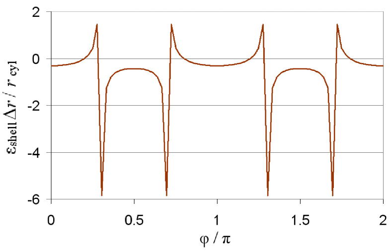
Figure 2: $\epsilon_{\mathrm{shell}}\,\mathrm{\Delta}r/r_{\mathrm{cyl}}$ vs. angle for $H_{f}=2$, $r_{f}=1.2r_{\mathrm{cyl}}$ and $\mathrm{\Delta}\phi=2\pi/16$, $n_{\max}=12$ harmonics.

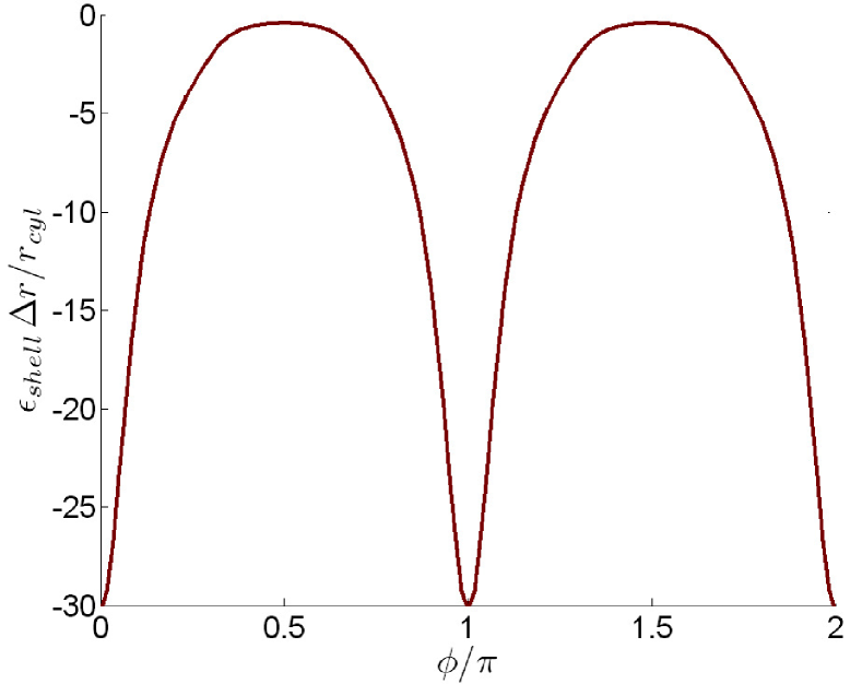
Figure 3: $\epsilon_{\mathrm{shell}}\,\mathrm{\Delta}r/r_{\mathrm{cyl}}$ vs. angle for $H_{f}=10$, $r_{f}=1.2r_{\mathrm{cyl}}$ and $\mathrm{\Delta}\phi=2\pi/18$, $n_{\max}=20$ harmonics.

Higher values of $H_{f}$ require a strong plasmonic resonance with $\epsilon_{\mathrm{shell}}(\phi)$ consistently negative (Fig. 3, $H_{f}=10$, $n_{\max}=20$ and $\mathrm{\Delta}\phi=2\pi/18$). Here the derivative $g^{\prime}(\phi)$ was chosen as a Gaussian peak $g^{\prime}(\phi)=\exp(-\phi^{2}/\mathrm{\Delta}\phi^{2})$, where parameter $\mathrm{\Delta}\phi$ controls the width of the peak. This angular distribution of the magnetic field leads to a respective peak in $E_{r}(\phi)$ (Fig. 4 and Fig. 5). The fields were computed semi-analytically with (3)–(5) and also numerically using finite-difference (FD) analysis on regular polar grids. The semi-analytical solution in its present form is valid only in the absence of losses ($\epsilon^{\prime\prime}_{\mathrm{shell}}=0$) and, as Fig. 5 shows, is in that case close to the numerical solution. (The discrepancy is due primarily to the finite thickness of the shell $\mathrm{\Delta}r=0.02r_{\mathrm{cyl}}$ in FD simulations, and to the limited number of cylindrical harmonics in the semi-analytical treatment.) Losses affect the amplitude of the peak but not its sharpness (Fig. 5, $\epsilon^{\prime\prime}_{\mathrm{shell}}=0.1$). Convergence of FD results was verified by running the simulation on different grids (e.g. almost coinciding dashed and dotted lines corresponding to two different grids, Fig. 5).

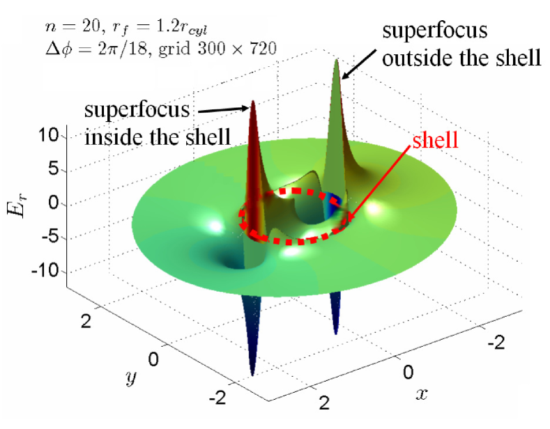
Figure 4: Surface plot of $E_{r}$ reveals “super-focuses” inside and outside the shell. No losses. Parameters: $H_{f}=10$, $n_{\max}=20$ harmonics, $r_{f}=1.2r_{\mathrm{cyl}}$, $\mathrm{\Delta}\phi=2\pi/18$, FD grid $n_{r}\times n_{\phi}=300\times 720$.

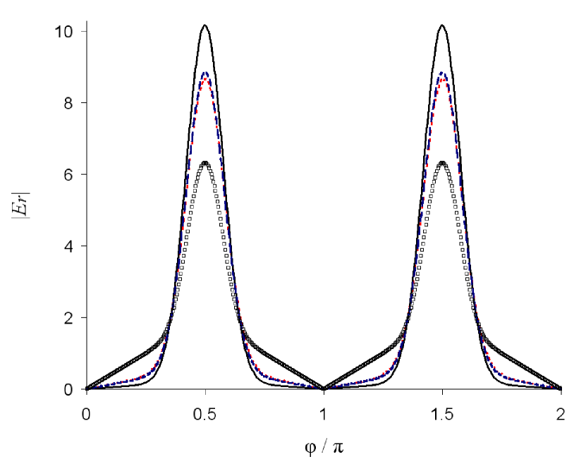
Figure 5: $E_{r}$ vs. angle at the radius of the focus $r_{f}=1.2r_{\mathrm{cyl}}$. Same parameters as in the previous figure. Losses ($\epsilon^{\prime\prime}_{\mathrm{shell}}=0.1$) reduce the magnitude of the focusing peak but do not significantly affect its sharpness. Solid line: semi-analytical solution (20 harmonics). Dashed and dotted lines on top of one another: no losses, FD solutions for grids $n_{r}\times n_{\phi}=150\times 480$ and $300\times 720$. Empty squares: FD solution, $\epsilon^{\prime\prime}=0.1$, grid $150\times 480$.

In summary, “superfocusing” of light by nanoshell scatterers, with the sharpness of the focus in principle unlimited, has been demonstrated analytically and numerically. The shell is designed in two stages: (i) analytical continuation of the desired behavior of the field at the focus to the boundary of the scatterer; (ii) finding the distribution of the dielectric permittivity and thickness of the shell that would produce the required field on the surface. Recently proposed focusing by “superoscillations” Zheludev-Huang09 also falls into this framework, but with the waveform at the focus cleverly chosen to contain only traveling wave components.

The procedure can be generalized to arbitrary shapes of the scattering shell and to 3D by still using cylindrical / spherical harmonic expansion in the outside region (as in T-matrix methods Mishchenko-Travis-Lacis02 ) and numerical methods (e.g. FEM) inside.

Numerical examples of very sharp focusing presented in this Letter should be viewed primarily as proof of concept; further improvement of the focusing effects should definitely be possible with sophisticated numerical optimization techniques (e.g. adaptive goal-oriented finite element analysis Oden-Prudhomme-01 ) that will treat not only the physical properties of the shell but also its geometric shape as adjustable parameters. Finally, it would be interesting to explore similar ideas for superfocusing of surface plasmon polaritons propagating on surfaces with judiciously chosen patterns Zheludev-Huang09 .

I thank N. I. Zheludev, S. I. Bozhevolnyi and the anonymous reviewer for very interesting and helpful comments.

References

- [1] N.I. Zheludev. What diffraction limit? Nature Materials, 7(6):420–422, 2008.
- [2] K.L. Tsakmakidis, A.D. Boardman & O. Hess. ‘Trapped rainbow’ storage of light in metamaterials. Nature, 450(7168):397–401, 2007.
- [3] J. Pendry. Time reversal and negative refraction. Science, 322(5898):71–73, 2008.
- [4] N. Zheludev, F. Huang. Superresolution without evanescent waves. Nano Letters, in press. N. I. Zheludev, private communication, Jan 2009.
- [5] J.B. Pendry and D.R. Smith. Reversing light with negative refraction. Phys. Today, 57:37–43, 2004.
- [6] J. Dai, F. Čajko, I. Tsukerman, and M.I. Stockman. Electrodynamic effects in plasmonic nanolenses. Phys. Rev. B, 77:115419-1-5, 2008.
- [7] R. Merlin. Radiationless electromagnetic interference: Evanescent-field lenses and perfect focusing. Science, 317(5840):927–929, 2007.
- [8] A. Grbic, L. Jiang, R. Merlin. Near-field plates: Subdiffraction focusing with patterned surfaces. Science, 320 (5875):511–513, 2008.
- [9] L.E. Helseth. The almost perfect lens and focusing of evanescent waves. Opt Comm, 281(8):1981–1985, 2008.
- [10] S. I. Bozhevolnyi and B. Vohnsen. Near-field optical holography. Phys. Rev. Lett., 77:3351–3354, 1996. S.I. Bozhevolnyi, private communication, Jan 2009.
- [11] G. Della Valle, T. Sondergaard, and S. I. Bozhevolnyi, Plasmon-polariton nano-strip resonators: from visible to infra-red, Opt. Express 16, 6867–6876, 2008.
- [12] I. D. Mayergoyz, D. R. Fredkin and Z. Zhang, Electrostatic (plasmon) resonances in nanoparticles, Phys. Rev. B 72, 155412, 2005.
- [13] G. Shvets and Y. A. Urzhumov. Engineering the electromagnetic properties of periodic nanostructures using electrostatic resonances. Phys. Rev. Lett., 24:243902-1–4, 2004.
- [14] J.T. Oden, S. Prudhomme. Goal-oriented error estimation and adaptivity for the finite element method. Computers & Mathematics with Applications, 41(5–6):735–756, 2001.
- [15] M. I. Mishchenko, L. D. Travis, and A. A. Lacis, Scattering, Absorption, and Emission of Light by Small Particles, Cambridge University Press, Cambridge, 2002.