2 Singularity analysis
In [10 ] we obtained the exponential generating function
∑ n = 0 ∞ P n ( x ) z n n ! = exp { 1 2 S 2 [ N ( x ) + z N ′ ( x ) ] − x 2 2 } , superscript subscript 𝑛 0 subscript 𝑃 𝑛 𝑥 superscript 𝑧 𝑛 𝑛 1 2 superscript 𝑆 2 delimited-[] 𝑁 𝑥 𝑧 superscript 𝑁 ′ 𝑥 superscript 𝑥 2 2 \sum_{n=0}^{\infty}P_{n}(x)\frac{z^{n}}{n!}=\exp\left\{\frac{1}{2}S^{2}[N(x)+zN^{\prime}(x)]-\frac{x^{2}}{2}\right\},
which implies that
P n ( x ) = e − x 2 / 2 n ! 2 π i ∮ | z | < r exp { 1 2 S 2 [ N ( x ) + z N ′ ( x ) ] } d z z n + 1 , subscript 𝑃 𝑛 𝑥 superscript 𝑒 superscript 𝑥 2 2 𝑛 2 𝜋 i subscript contour-integral 𝑧 𝑟 1 2 superscript 𝑆 2 delimited-[] 𝑁 𝑥 𝑧 superscript 𝑁 ′ 𝑥 𝑑 𝑧 superscript 𝑧 𝑛 1 P_{n}(x)=e^{-x^{2}/2}\frac{n!}{2\pi\mathrm{i}}\oint\limits_{\left|z\right|<r}\exp\left\{\frac{1}{2}S^{2}[N(x)+zN^{\prime}(x)]\right\}\frac{dz}{z^{n+1}},
where the integration contour is a small loop around the origin in the complex
plane. Using (4
P n ( x ) subscript 𝑃 𝑛 𝑥 \displaystyle P_{n}(x) = e − x 2 / 2 n ! 2 π i ∮ | z | < r 1 2 π S ′ [ N ( x ) + z N ′ ( x ) ] d z z n + 1 absent superscript 𝑒 superscript 𝑥 2 2 𝑛 2 𝜋 i subscript contour-integral 𝑧 𝑟 1 2 𝜋 superscript 𝑆 ′ delimited-[] 𝑁 𝑥 𝑧 superscript 𝑁 ′ 𝑥 𝑑 𝑧 superscript 𝑧 𝑛 1 \displaystyle=e^{-x^{2}/2}\frac{n!}{2\pi\mathrm{i}}\oint\limits_{\left|z\right|<r}\frac{1}{\sqrt{2\pi}}S^{\prime}[N(x)+zN^{\prime}(x)]\frac{dz}{z^{n+1}}
= e − x 2 / 2 1 2 π N ′ ( x ) n ! 2 π i ∮ | z | < r 1 z n + 1 𝑑 S [ N ( x ) + z N ′ ( x ) ] absent superscript 𝑒 superscript 𝑥 2 2 1 2 𝜋 superscript 𝑁 ′ 𝑥 𝑛 2 𝜋 i subscript contour-integral 𝑧 𝑟 1 superscript 𝑧 𝑛 1 differential-d 𝑆 delimited-[] 𝑁 𝑥 𝑧 superscript 𝑁 ′ 𝑥 \displaystyle=e^{-x^{2}/2}\frac{1}{\sqrt{2\pi}N^{\prime}(x)}\frac{n!}{2\pi\mathrm{i}}\oint\limits_{\left|z\right|<r}\frac{1}{z^{n+1}}dS[N(x)+zN^{\prime}(x)]
= n ! 2 π i ∮ | z | < r n + 1 z n + 2 S [ N ( x ) + z N ′ ( x ) ] 𝑑 z absent 𝑛 2 𝜋 i subscript contour-integral 𝑧 𝑟 𝑛 1 superscript 𝑧 𝑛 2 𝑆 delimited-[] 𝑁 𝑥 𝑧 superscript 𝑁 ′ 𝑥 differential-d 𝑧 \displaystyle=\frac{n!}{2\pi\mathrm{i}}\oint\limits_{\left|z\right|<r}\frac{n+1}{z^{n+2}}S[N(x)+zN^{\prime}(x)]dz
and therefore
P n ( x ) = ( n + 1 ) ! 2 π i ∮ | z | < r S [ N ( x ) + z N ′ ( x ) ] d z z n + 2 . subscript 𝑃 𝑛 𝑥 𝑛 1 2 𝜋 i subscript contour-integral 𝑧 𝑟 𝑆 delimited-[] 𝑁 𝑥 𝑧 superscript 𝑁 ′ 𝑥 𝑑 𝑧 superscript 𝑧 𝑛 2 P_{n}(x)=\frac{\left(n+1\right)!}{2\pi\mathrm{i}}\oint\limits_{\left|z\right|<r}S[N(x)+zN^{\prime}(x)]\frac{dz}{z^{n+2}}. (9)
Since S ( x ) 𝑆 𝑥 S(x) x = 0 𝑥 0 x=0 x = 1 , 𝑥 1 x=1,
Z 1 ( x ) = 1 − N ( x ) N ′ ( x ) , Z 0 ( x ) = − N ( x ) N ′ ( x ) . formulae-sequence subscript 𝑍 1 𝑥 1 𝑁 𝑥 superscript 𝑁 ′ 𝑥 subscript 𝑍 0 𝑥 𝑁 𝑥 superscript 𝑁 ′ 𝑥 Z_{1}(x)=\frac{1-N(x)}{N^{\prime}(x)},\quad Z_{0}(x)=-\frac{N(x)}{N^{\prime}(x)}.
We have
Z 1 ( − x ) = − 2 π exp ( x 2 2 ) − Z 1 ( x ) subscript 𝑍 1 𝑥 2 𝜋 superscript 𝑥 2 2 subscript 𝑍 1 𝑥 Z_{1}(-x)=-\sqrt{2\pi}\exp\left(\frac{x^{2}}{2}\right)-Z_{1}(x) (10)
and
Z 1 ( x ) subscript 𝑍 1 𝑥 \displaystyle Z_{1}(x) = x − 1 + O ( x − 3 ) , x → ∞ , formulae-sequence absent superscript 𝑥 1 𝑂 superscript 𝑥 3 → 𝑥 \displaystyle=x^{-1}+O\left(x^{-3}\right),\quad x\rightarrow\infty,
Z 0 ( x ) subscript 𝑍 0 𝑥 \displaystyle\quad Z_{0}(x) = − 2 π exp ( x 2 2 ) + x − 1 + O ( x − 3 ) , x → ∞ . formulae-sequence absent 2 𝜋 superscript 𝑥 2 2 superscript 𝑥 1 𝑂 superscript 𝑥 3 → 𝑥 \displaystyle=-\sqrt{2\pi}\exp\left(\frac{x^{2}}{2}\right)+x^{-1}+O\left(x^{-3}\right),\quad x\rightarrow\infty.
Changing variables to
w = [ z − Z 1 ( x ) ] N ′ ( x ) 𝑤 delimited-[] 𝑧 subscript 𝑍 1 𝑥 superscript 𝑁 ′ 𝑥 w=\left[z-Z_{1}(x)\right]N^{\prime}(x)
in (9
P n ( x ) = 1 N ′ ( x ) ( n + 1 ) ! 2 π i ∮ C S ( w + 1 ) [ w N ′ ( x ) + Z 1 ( x ) ] − ( n + 2 ) 𝑑 w , subscript 𝑃 𝑛 𝑥 1 superscript 𝑁 ′ 𝑥 𝑛 1 2 𝜋 i subscript contour-integral 𝐶 𝑆 𝑤 1 superscript delimited-[] 𝑤 superscript 𝑁 ′ 𝑥 subscript 𝑍 1 𝑥 𝑛 2 differential-d 𝑤 P_{n}(x)=\frac{1}{N^{\prime}(x)}\frac{\left(n+1\right)!}{2\pi\mathrm{i}}\oint\limits_{C}S\left(w+1\right)\left[\frac{w}{N^{\prime}(x)}+Z_{1}(x)\right]^{-(n+2)}dw,
or,
P n ( x ) = π e x 2 / 2 ( n + 1 ) ! 2 π i ∮ C 𝒥 ( w + 1 ) [ π 2 e x 2 / 2 w + Z 1 ( x ) ] n + 2 𝑑 w , subscript 𝑃 𝑛 𝑥 𝜋 superscript 𝑒 superscript 𝑥 2 2 𝑛 1 2 𝜋 i subscript contour-integral 𝐶 𝒥 𝑤 1 superscript delimited-[] 𝜋 2 superscript 𝑒 superscript 𝑥 2 2 𝑤 subscript 𝑍 1 𝑥 𝑛 2 differential-d 𝑤 P_{n}(x)=\sqrt{\pi}e^{x^{2}/2}\frac{\left(n+1\right)!}{2\pi\mathrm{i}}\oint\limits_{C}\frac{\mathcal{J}\left(w+1\right)}{\left[\sqrt{\frac{\pi}{2}}e^{x^{2}/2}w+Z_{1}(x)\right]^{n+2}}dw, (11)
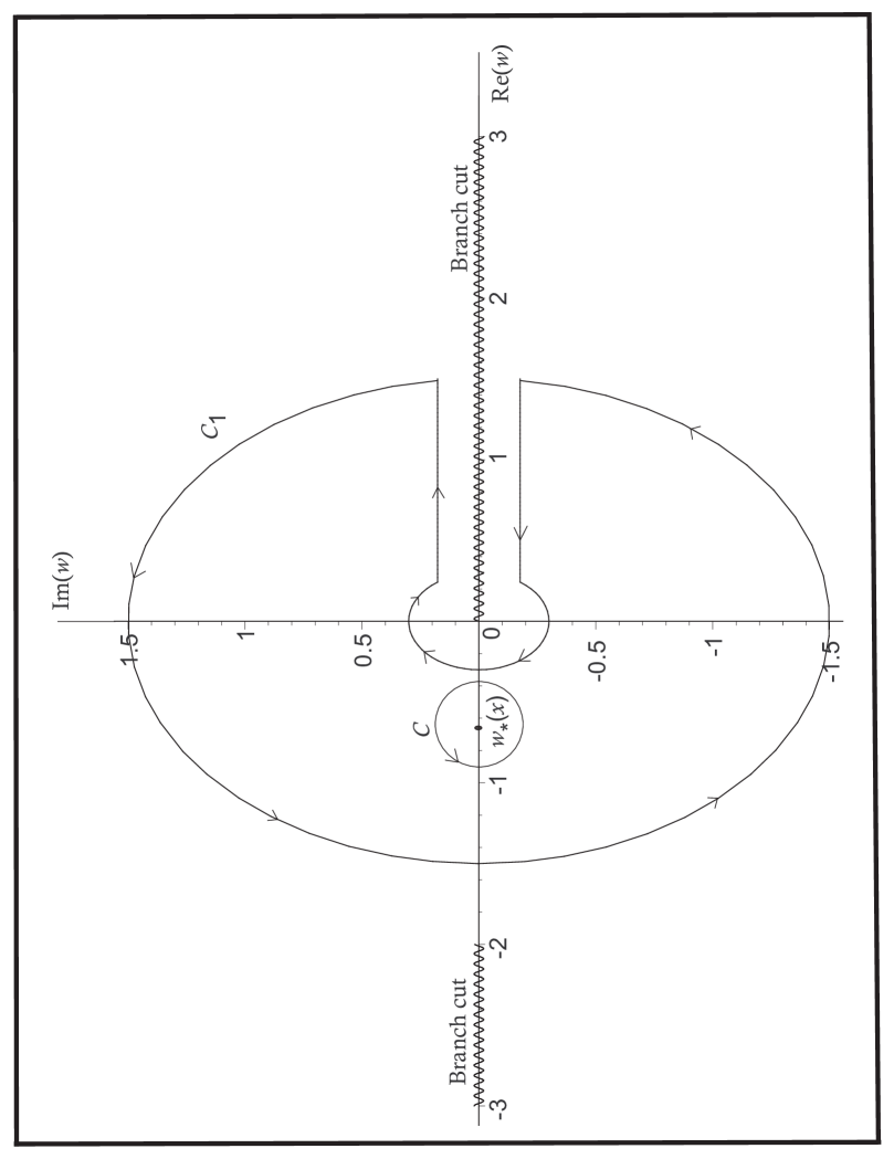
where C 𝐶 C w = w ∗ ( x ) 𝑤 superscript 𝑤 ∗ 𝑥 w=w^{\ast}(x)
w ∗ ( x ) = − 2 π e − x 2 / 2 Z 1 ( x ) . superscript 𝑤 ∗ 𝑥 2 𝜋 superscript 𝑒 superscript 𝑥 2 2 subscript 𝑍 1 𝑥 w^{\ast}(x)=-\sqrt{\frac{2}{\pi}}e^{-x^{2}/2}Z_{1}(x).
To expand (11 n → ∞ → 𝑛 n\rightarrow\infty x ∈ ( 0 , ∞ ) , 𝑥 0 x\in\left(0,\infty\right), 𝒥 ( w ) 𝒥 𝑤 \mathcal{J(}w) w = ± 1 . 𝑤 plus-or-minus 1 w=\pm 1. 1
w = 2 π ∫ 0 𝒥 e − t 2 𝑑 t = 1 − e − 𝒥 2 [ 1 π 𝒥 + O ( 𝒥 − 3 ) ] , 𝒥 → ∞ , formulae-sequence 𝑤 2 𝜋 superscript subscript 0 𝒥 superscript 𝑒 superscript 𝑡 2 differential-d 𝑡 1 superscript 𝑒 superscript 𝒥 2 delimited-[] 1 𝜋 𝒥 𝑂 superscript 𝒥 3 → 𝒥 w=\frac{2}{\sqrt{\pi}}\int\limits_{0}^{\mathcal{J}}e^{-t^{2}}dt=1-e^{-\mathcal{J}^{2}}\left[\frac{1}{\sqrt{\pi}\mathcal{J}}+O\left(\mathcal{J}^{-3}\right)\right],\quad\mathcal{J}\rightarrow\infty,
so that
𝒥 ( w ) ∼ − ln ( 1 − w ) , w → 1 − formulae-sequence similar-to 𝒥 𝑤 1 𝑤 → 𝑤 superscript 1 \mathcal{J(}w)\sim\sqrt{-\ln(1-w)},\quad w\rightarrow 1^{-}
and by symmetry we have
𝒥 ( w ) ∼ − − ln ( 1 + w ) , w → − 1 + . formulae-sequence similar-to 𝒥 𝑤 1 𝑤 → 𝑤 superscript 1 \mathcal{J(}w)\sim-\sqrt{-\ln(1+w)},\quad w\rightarrow-1^{+}.
The integrand in (11 w = 0 𝑤 0 w=0 w = − 2 , 𝑤 2 w=-2, x > 0 , 𝑥 0 x>0, w ∗ ( x ) . superscript 𝑤 ∗ 𝑥 w^{\ast}(x). 11 w = 0 𝑤 0 w=0 w = δ / n 𝑤 𝛿 𝑛 w=\delta/n
[ Z 1 ( x ) + π 2 e x 2 / 2 δ n ] − ( n + 2 ) ∼ [ Z 1 ( x ) ] − ( n + 2 ) exp [ − π 2 e x 2 / 2 δ Z 1 ( x ) ] . similar-to superscript delimited-[] subscript 𝑍 1 𝑥 𝜋 2 superscript 𝑒 superscript 𝑥 2 2 𝛿 𝑛 𝑛 2 superscript delimited-[] subscript 𝑍 1 𝑥 𝑛 2 𝜋 2 superscript 𝑒 superscript 𝑥 2 2 𝛿 subscript 𝑍 1 𝑥 \left[Z_{1}(x)+\sqrt{\frac{\pi}{2}}e^{x^{2}/2}\frac{\delta}{n}\right]^{-(n+2)}\sim\left[Z_{1}(x)\right]^{-(n+2)}\exp\left[-\sqrt{\frac{\pi}{2}}e^{x^{2}/2}\frac{\delta}{Z_{1}(x)}\right]. (12)
Then, we deform the contour C 𝐶 C 11 C 1 subscript 𝐶 1 C_{1} w = 0 𝑤 0 w=0 1
P n ( x ) subscript 𝑃 𝑛 𝑥 \displaystyle P_{n}(x) ∼ ( n + 1 ) ! π e x 2 / 2 [ Z 1 ( x ) ] − ( n + 2 ) 1 n similar-to absent 𝑛 1 𝜋 superscript 𝑒 superscript 𝑥 2 2 superscript delimited-[] subscript 𝑍 1 𝑥 𝑛 2 1 𝑛 \displaystyle\sim\left(n+1\right)!\sqrt{\pi}e^{x^{2}/2}\left[Z_{1}(x)\right]^{-(n+2)}\frac{1}{n} (13)
× 1 2 π i ∫ 0 ∞ ( Υ + − Υ − ) exp [ − π 2 e x 2 / 2 Z 1 ( x ) δ ] 𝑑 δ , absent 1 2 𝜋 i superscript subscript 0 superscript Υ superscript Υ 𝜋 2 superscript 𝑒 superscript 𝑥 2 2 subscript 𝑍 1 𝑥 𝛿 differential-d 𝛿 \displaystyle\times\frac{1}{2\pi\mathrm{i}}\int\limits_{0}^{\infty}\left(\Upsilon^{+}-\Upsilon^{-}\right)\exp\left[-\sqrt{\frac{\pi}{2}}\frac{e^{x^{2}/2}}{Z_{1}(x)}\delta\right]d\delta,
where
Υ ± ( δ , n ) = ± i π − ln ( δ ) + ln ( n ) . superscript Υ plus-or-minus 𝛿 𝑛 plus-or-minus i 𝜋 𝛿 𝑛 \Upsilon^{\pm}(\delta,n)=\sqrt{\pm\mathrm{i}\pi-\ln\left(\delta\right)+\ln\left(n\right)}.
Here Υ ± ( δ , n ) superscript Υ plus-or-minus 𝛿 𝑛 \Upsilon^{\pm}(\delta,n) 𝒥 ( w + 1 ) 𝒥 𝑤 1 \mathcal{J(}w+1) w → 0 , → 𝑤 0 w\rightarrow 0, 1
Figure 1: A sketch of the contours C 𝐶 C C 1 subscript 𝐶 1 C_{1}
For n 𝑛 n
Υ + ( δ , n ) − Υ − ( δ , n ) ∼ π i ln ( n ) similar-to superscript Υ 𝛿 𝑛 superscript Υ 𝛿 𝑛 𝜋 i 𝑛 \Upsilon^{+}(\delta,n)-\Upsilon^{-}(\delta,n)\sim\frac{\pi\mathrm{i}}{\sqrt{\ln\left(n\right)}}
and then evaluating the elementary integral in (13 P n ( x ) ∼ Ψ 1 ( x , n ) similar-to subscript 𝑃 𝑛 𝑥 subscript Ψ 1 𝑥 𝑛 P_{n}(x)\sim\Psi_{1}(x,n) n → ∞ → 𝑛 n\rightarrow\infty
Ψ 1 ( x , n ) = n ! 2 ln ( n ) [ Z 1 ( x ) ] − ( n + 1 ) = n ! 2 ln ( n ) [ e − x 2 / 2 ζ ( x ) ] n + 1 subscript Ψ 1 𝑥 𝑛 𝑛 2 𝑛 superscript delimited-[] subscript 𝑍 1 𝑥 𝑛 1 𝑛 2 𝑛 superscript delimited-[] superscript 𝑒 superscript 𝑥 2 2 𝜁 𝑥 𝑛 1 \Psi_{1}(x,n)=\frac{n!}{\sqrt{2\ln\left(n\right)}}\left[Z_{1}(x)\right]^{-\left(n+1\right)}=\frac{n!}{\sqrt{2\ln\left(n\right)}}\left[\frac{e^{-x^{2}/2}}{\zeta\left(x\right)}\right]^{n+1} (14)
and
ζ ( x ) = π 2 [ 1 − erf ( x 2 ) ] ∼ exp ( − x 2 2 ) [ x − 1 + O ( x − 3 ) ] , x → ∞ . formulae-sequence 𝜁 𝑥 𝜋 2 delimited-[] 1 erf 𝑥 2 similar-to superscript 𝑥 2 2 delimited-[] superscript 𝑥 1 𝑂 superscript 𝑥 3 → 𝑥 \zeta\left(x\right)=\sqrt{\frac{\pi}{2}}\left[1-\operatorname*{erf}\left(\frac{x}{\sqrt{2}}\right)\right]\sim\exp\left(-\frac{x^{2}}{2}\right)\left[x^{-1}+O\left(x^{-3}\right)\right],\quad x\rightarrow\infty. (15)
In Figure 2 ln [ P 40 ( x ) / 40 ! ] subscript 𝑃 40 𝑥 40 \ln\left[P_{40}(x)/40!\right] ln [ Ψ 1 ( x , 40 ) / 40 ! ] subscript Ψ 1 𝑥 40 40 \ln\left[\Psi_{1}(x,40)/40!\right] x = O ( 1 ) 𝑥 𝑂 1 x=O(1) x → ∞ . → 𝑥 x\rightarrow\infty. n → ∞ → 𝑛 n\rightarrow\infty 0 < x < ∞ . 0 𝑥 0<x<\infty. x → 0 → 𝑥 0 x\rightarrow 0 x → ∞ , → 𝑥 x\rightarrow\infty,
Figure 2: A plot of ln [ P 40 ( x ) / 40 ! ] subscript 𝑃 40 𝑥 40 \ln\left[P_{40}(x)/40!\right] ln [ Ψ 1 ( x , 40 ) / 40 ! ] subscript Ψ 1 𝑥 40 40 \ln\left[\Psi_{1}(x,40)/40!\right]
When x → 0 , → 𝑥 0 x\rightarrow 0, x = O ( n − 1 ) , 𝑥 𝑂 superscript 𝑛 1 x=O\left(n^{-1}\right), w = 0 𝑤 0 w=0 w = − 2 𝑤 2 w=-2 w ∗ ( x ) . superscript 𝑤 ∗ 𝑥 w^{\ast}(x). x = y / n , 𝑥 𝑦 𝑛 x=y/n, y = O ( 1 ) , 𝑦 𝑂 1 y=O\left(1\right),
Z 1 ( x ) = Z 1 ( y n ) = π 2 − y n + O ( n − 2 ) , n → ∞ formulae-sequence subscript 𝑍 1 𝑥 subscript 𝑍 1 𝑦 𝑛 𝜋 2 𝑦 𝑛 𝑂 superscript 𝑛 2 → 𝑛 Z_{1}(x)=Z_{1}\left(\frac{y}{n}\right)=\sqrt{\frac{\pi}{2}}-\frac{y}{n}+O\left(n^{-2}\right),\quad n\rightarrow\infty (16)
and (14
P n ( x ) ∼ n ! 2 ln ( n ) ( 2 π ) n + 1 exp ( y 2 π ) . similar-to subscript 𝑃 𝑛 𝑥 𝑛 2 𝑛 superscript 2 𝜋 𝑛 1 𝑦 2 𝜋 P_{n}(x)\sim\frac{n!}{\sqrt{2\ln\left(n\right)}}\left(\sqrt{\frac{2}{\pi}}\right)^{n+1}\exp\left(y\sqrt{\frac{2}{\pi}}\right). (17)
But, to this we must add the contribution from w = − 2 , 𝑤 2 w=-2, y 𝑦 y − y 𝑦 -y ( − 1 ) n superscript 1 𝑛 \left(-1\right)^{n} 17
We note from (10
π 2 e x 2 / 2 w + Z 1 ( − x ) = π 2 e x 2 / 2 ( w + 2 ) − Z 1 ( x ) , 𝜋 2 superscript 𝑒 superscript 𝑥 2 2 𝑤 subscript 𝑍 1 𝑥 𝜋 2 superscript 𝑒 superscript 𝑥 2 2 𝑤 2 subscript 𝑍 1 𝑥 \sqrt{\frac{\pi}{2}}e^{x^{2}/2}w+Z_{1}(-x)=\sqrt{\frac{\pi}{2}}e^{x^{2}/2}\left(w+2\right)-Z_{1}(x),
so that the integrand in (11 ( x , w ) → ( − x , − 2 − w ) . → 𝑥 𝑤 𝑥 2 𝑤 \left(x,w\right)\rightarrow\left(-x,-2-w\right). n → ∞ → 𝑛 n\rightarrow\infty x = O ( n − 1 ) 𝑥 𝑂 superscript 𝑛 1 x=O\left(n^{-1}\right) P n ( x ) ∼ Ψ 2 ( x , n ) similar-to subscript 𝑃 𝑛 𝑥 subscript Ψ 2 𝑥 𝑛 P_{n}(x)\sim\Psi_{2}(x,n)
Ψ 2 ( y , n ) = n ! 2 ln ( n ) ( 2 π ) n + 1 [ exp ( y 2 π ) + ( − 1 ) n exp ( − y 2 π ) ] . subscript Ψ 2 𝑦 𝑛 𝑛 2 𝑛 superscript 2 𝜋 𝑛 1 delimited-[] 𝑦 2 𝜋 superscript 1 𝑛 𝑦 2 𝜋 \Psi_{2}(y,n)=\frac{n!}{\sqrt{2\ln\left(n\right)}}\left(\sqrt{\frac{2}{\pi}}\right)^{n+1}\left[\exp\left(y\sqrt{\frac{2}{\pi}}\right)+\left(-1\right)^{n}\exp\left(-y\sqrt{\frac{2}{\pi}}\right)\right]. (18)
As y → ∞ , → 𝑦 y\rightarrow\infty, 18 14 x → 0 . → 𝑥 0 x\rightarrow 0. 3 ln [ P 40 ( y 40 ) / 40 ! ] / ln [ Ψ 2 ( y , 40 ) / 40 ! ] subscript 𝑃 40 𝑦 40 40 subscript Ψ 2 𝑦 40 40 \ln\left[P_{40}\left(\frac{y}{40}\right)/40!\right]/\ln\left[\Psi_{2}(y,40)/40!\right] 18
Figure 3: A plot of the
ratio ln [ P 40 ( y 40 ) / 40 ! ] / ln [ Ψ 2 ( y , 40 ) / 40 ! ] subscript 𝑃 40 𝑦 40 40 subscript Ψ 2 𝑦 40 40 \ln\left[P_{40}\left(\frac{y}{40}\right)/40!\right]/\ln\left[\Psi_{2}(y,40)/40!\right]
Letting x → ∞ → 𝑥 x\rightarrow\infty 13 14
P n ( x ) ∼ n ! x n + 1 2 ln ( n ) , similar-to subscript 𝑃 𝑛 𝑥 𝑛 superscript 𝑥 𝑛 1 2 𝑛 P_{n}(x)\sim\frac{n!\,x^{n+1}}{\sqrt{2\ln(n)}},
which differs from (7 x 𝑥 x n 𝑛 n x → ∞ → 𝑥 x\rightarrow\infty x = O ( ln n ) . 𝑥 𝑂 𝑛 x=O\left(\sqrt{\ln n}\right). w = 0 𝑤 0 w=0 11 w ∗ ( x ) , superscript 𝑤 ∗ 𝑥 w^{\ast}(x),
w ∗ ( x ) ∼ − 2 x π , x → ∞ . formulae-sequence similar-to superscript 𝑤 ∗ 𝑥 2 𝑥 𝜋 → 𝑥 w^{\ast}(x)\sim-\frac{\sqrt{2}}{x\sqrt{\pi}},\quad x\rightarrow\infty.
we use the form (9 S [ N ( x ) + z N ′ ( x ) ] 𝑆 delimited-[] 𝑁 𝑥 𝑧 superscript 𝑁 ′ 𝑥 S[N(x)+zN^{\prime}(x)] z → 0 → 𝑧 0 z\rightarrow 0 x → ∞ . → 𝑥 x\rightarrow\infty. z = ξ / x 𝑧 𝜉 𝑥 z=\xi/x ξ = O ( 1 ) , 𝜉 𝑂 1 \xi=O(1),
S [ N ( x ) + z N ′ ( x ) ] = 2 𝒥 { 1 + 2 π [ z e − x 2 / 2 − ζ ( x ) ] } 𝑆 delimited-[] 𝑁 𝑥 𝑧 superscript 𝑁 ′ 𝑥 2 𝒥 1 2 𝜋 delimited-[] 𝑧 superscript 𝑒 superscript 𝑥 2 2 𝜁 𝑥 \displaystyle S[N(x)+zN^{\prime}(x)]=\sqrt{2}\mathcal{J}\left\{1+\sqrt{\frac{2}{\pi}}\left[ze^{-x^{2}/2}-\zeta\left(x\right)\right]\right\}
= 2 𝒥 [ 1 + 2 π e − x 2 / 2 ( z − 1 x + O ( x − 3 ) ) ] absent 2 𝒥 delimited-[] 1 2 𝜋 superscript 𝑒 superscript 𝑥 2 2 𝑧 1 𝑥 𝑂 superscript 𝑥 3 \displaystyle=\sqrt{2}\mathcal{J}\left[1+\sqrt{\frac{2}{\pi}}e^{-x^{2}/2}\left(z-\frac{1}{x}+O\left(x^{-3}\right)\right)\right]
∼ 2 − ln [ 2 π e − x 2 / 2 ( 1 x − z ) ] similar-to absent 2 2 𝜋 superscript 𝑒 superscript 𝑥 2 2 1 𝑥 𝑧 \displaystyle\sim\sqrt{2}\sqrt{-\ln\left[\sqrt{\frac{2}{\pi}}e^{-x^{2}/2}\left(\frac{1}{x}-z\right)\right]}
∼ 2 x 2 2 + ln ( x ) − 1 2 ln ( 2 π ) − ln ( 1 − ξ ) . similar-to absent 2 superscript 𝑥 2 2 𝑥 1 2 2 𝜋 1 𝜉 \displaystyle\sim\sqrt{2}\sqrt{\frac{x^{2}}{2}+\ln(x)-\frac{1}{2}\ln\left(\frac{2}{\pi}\right)-\ln\left(1-\xi\right)}.
Thus, we have
P n ( x ) ∼ 2 ( n + 1 ) ! x n + 1 2 π i ∮ C 1 x 2 2 + ln ( x 1 − ξ ) − 1 2 ln ( 2 π ) d ξ ξ n + 2 . similar-to subscript 𝑃 𝑛 𝑥 2 𝑛 1 superscript 𝑥 𝑛 1 2 𝜋 i subscript contour-integral subscript 𝐶 1 superscript 𝑥 2 2 𝑥 1 𝜉 1 2 2 𝜋 𝑑 𝜉 superscript 𝜉 𝑛 2 P_{n}(x)\sim\frac{\sqrt{2}\left(n+1\right)!x^{n+1}}{2\pi\mathrm{i}}\oint\limits_{C_{1}}\sqrt{\frac{x^{2}}{2}+\ln\left(\frac{x}{1-\xi}\right)-\frac{1}{2}\ln\left(\frac{2}{\pi}\right)}\frac{d\xi}{\xi^{n+2}}. (19)
Here the contour C 1 subscript 𝐶 1 C_{1} ξ = 0 . 𝜉 0 \xi=0. ξ = 1 𝜉 1 \xi=1 n → ∞ . → 𝑛 n\rightarrow\infty. 1
P n ( x ) ∼ n ! x n + 1 2 1 x 2 2 + ln ( n x ) − 1 2 ln ( 2 π ) . similar-to subscript 𝑃 𝑛 𝑥 𝑛 superscript 𝑥 𝑛 1 2 1 superscript 𝑥 2 2 𝑛 𝑥 1 2 2 𝜋 P_{n}(x)\sim\frac{n!x^{n+1}}{\sqrt{2}}\frac{1}{\sqrt{\frac{x^{2}}{2}+\ln(nx)-\frac{1}{2}\ln\left(\frac{2}{\pi}\right)}}. (20)
For x >> ln ( n ) much-greater-than 𝑥 𝑛 x>>\sqrt{\ln(n)} 7
By examining (14 20
P n ( x ) ∼ Ψ 3 ( x , n ) = n ! x 2 + 2 ln ( n x ) − ln ( 2 π ) [ e − x 2 / 2 ζ ( x ) ] n + 1 , similar-to subscript 𝑃 𝑛 𝑥 subscript Ψ 3 𝑥 𝑛 𝑛 superscript 𝑥 2 2 𝑛 𝑥 2 𝜋 superscript delimited-[] superscript 𝑒 superscript 𝑥 2 2 𝜁 𝑥 𝑛 1 P_{n}(x)\sim\Psi_{3}(x,n)=\frac{n!}{\sqrt{x^{2}+2\ln(nx)-\ln\left(\frac{2}{\pi}\right)}}\left[\frac{e^{-x^{2}/2}}{\zeta\left(x\right)}\right]^{n+1}, (21)
which is more uniform in x 𝑥 x x = O ( 1 ) 𝑥 𝑂 1 x=O(1) x = O ( ln n ) 𝑥 𝑂 𝑛 x=O\left(\sqrt{\ln n}\right) n 𝑛 n x → ∞ → 𝑥 x\rightarrow\infty n 𝑛 n 18 n 𝑛 n x 𝑥 x 4 ln [ P 40 ( x ) / 40 ! ] subscript 𝑃 40 𝑥 40 \ln\left[P_{40}(x)/40!\right] ln [ Ψ 3 ( x , 40 ) / 40 ! ] subscript Ψ 3 𝑥 40 40 \ln\left[\Psi_{3}(x,40)/40!\right] 21 14 x . 𝑥 x.
Figure 4: A plot of ln [ P 40 ( x ) / 40 ! ] subscript 𝑃 40 𝑥 40 \ln\left[P_{40}(x)/40!\right] ln [ Ψ 3 ( x , 40 ) / 40 ! ] subscript Ψ 3 𝑥 40 40 \ln\left[\Psi_{3}(x,40)/40!\right]
3 WKB analysis
We shall now rederive the results in the previous section by using only the
recurrence (6 7 6 P n ( x ) = n ! P ¯ n ( x ) , subscript 𝑃 𝑛 𝑥 𝑛 subscript ¯ 𝑃 𝑛 𝑥 P_{n}(x)=n!\overline{P}_{n}(x),
P ¯ n ( x ) ∼ exp [ ( n + 1 ) A ( x ) ] B ( x , n ) , n → ∞ . formulae-sequence similar-to subscript ¯ 𝑃 𝑛 𝑥 𝑛 1 𝐴 𝑥 𝐵 𝑥 𝑛 → 𝑛 \overline{P}_{n}(x)\sim\exp\left[\left(n+1\right)A(x)\right]B(x,n),\quad n\rightarrow\infty. (22)
Thus, we are assuming an exponential dependence on n 𝑛 n B ( x , n ) . 𝐵 𝑥 𝑛 B(x,n). 22 6
e A ( x ) [ B ( x , n ) + ∂ ∂ n B ( x , n ) ] + O ( ∂ 2 B ∂ n 2 ) superscript 𝑒 𝐴 𝑥 delimited-[] 𝐵 𝑥 𝑛 𝑛 𝐵 𝑥 𝑛 𝑂 superscript 2 𝐵 superscript 𝑛 2 \displaystyle e^{A(x)}\left[B(x,n)+\frac{\partial}{\partial n}B(x,n)\right]+O\left(\frac{\partial^{2}B}{\partial n^{2}}\right)
= [ x + A ′ ( x ) ] B ( x , n ) + 1 n + 1 ∂ ∂ x B ( x , n ) . absent delimited-[] 𝑥 superscript 𝐴 ′ 𝑥 𝐵 𝑥 𝑛 1 𝑛 1 𝑥 𝐵 𝑥 𝑛 \displaystyle=\left[x+A^{\prime}(x)\right]B(x,n)+\frac{1}{n+1}\frac{\partial}{\partial x}B(x,n).
Expecting that ∂ B ∂ n = o ( B ) 𝐵 𝑛 𝑜 𝐵 \frac{\partial B}{\partial n}=o\left(B\right) ∂ 2 B ∂ n 2 = o ( ∂ B ∂ n ) , superscript 2 𝐵 superscript 𝑛 2 𝑜 𝐵 𝑛 \frac{\partial^{2}B}{\partial n^{2}}=o\left(\frac{\partial B}{\partial n}\right),
e A ( x ) = x + A ′ ( x ) superscript 𝑒 𝐴 𝑥 𝑥 superscript 𝐴 ′ 𝑥 e^{A(x)}=x+A^{\prime}(x) (23)
and
e A ( x ) ∂ ∂ n B ( x , n ) = 1 n + 1 ∂ ∂ x B ( x , n ) ∼ 1 n ∂ ∂ x B ( x , n ) . superscript 𝑒 𝐴 𝑥 𝑛 𝐵 𝑥 𝑛 1 𝑛 1 𝑥 𝐵 𝑥 𝑛 similar-to 1 𝑛 𝑥 𝐵 𝑥 𝑛 e^{A(x)}\frac{\partial}{\partial n}B(x,n)=\frac{1}{n+1}\frac{\partial}{\partial x}B(x,n)\sim\frac{1}{n}\frac{\partial}{\partial x}B(x,n). (24)
To solve (23
A ( x ) = − x 2 2 + a ( x ) 𝐴 𝑥 superscript 𝑥 2 2 𝑎 𝑥 A(x)=-\frac{x^{2}}{2}+a(x)
to find that
a ′ ( x ) = e − x 2 / 2 e a ( x ) . superscript 𝑎 ′ 𝑥 superscript 𝑒 superscript 𝑥 2 2 superscript 𝑒 𝑎 𝑥 a^{\prime}(x)=e^{-x^{2}/2}e^{a(x)}.
Solving this separable ODE leads to
A ( x ) = − x 2 2 − ln [ ζ ( x ) + k ] , 𝐴 𝑥 superscript 𝑥 2 2 𝜁 𝑥 𝑘 A(x)=-\frac{x^{2}}{2}-\ln\left[\zeta\left(x\right)+k\right], (25)
where k 𝑘 k k , 𝑘 k, 22 x → ∞ , → 𝑥 x\rightarrow\infty, 7 n → ∞ . → 𝑛 n\rightarrow\infty. 22
P ¯ n ( x ) ∼ x n = exp [ n ln ( x ) ] , x → ∞ , formulae-sequence similar-to subscript ¯ 𝑃 𝑛 𝑥 superscript 𝑥 𝑛 𝑛 𝑥 → 𝑥 \overline{P}_{n}(x)\sim x^{n}=\exp\left[n\ln(x)\right],\quad x\rightarrow\infty,
so that
A ( x ) ∼ ln ( x ) , x → ∞ . formulae-sequence similar-to 𝐴 𝑥 𝑥 → 𝑥 A(x)\sim\ln(x),\quad x\rightarrow\infty.
In view of (25 k = 0 𝑘 0 k=0 15
A ( x ) = − ln [ e x 2 / 2 ζ ( x ) ] ∼ ln ( x ) , x → ∞ . formulae-sequence 𝐴 𝑥 superscript 𝑒 superscript 𝑥 2 2 𝜁 𝑥 similar-to 𝑥 → 𝑥 A(x)=-\ln\left[e^{x^{2}/2}\zeta\left(x\right)\right]\sim\ln(x),\quad x\rightarrow\infty. (26)
We next analyze (24 26 e A ( x ) , superscript 𝑒 𝐴 𝑥 e^{A(x)},
e − x 2 / 2 ζ ( x ) ∂ ∂ n B ( x , n ) = 1 n ∂ ∂ x B ( x , n ) . superscript 𝑒 superscript 𝑥 2 2 𝜁 𝑥 𝑛 𝐵 𝑥 𝑛 1 𝑛 𝑥 𝐵 𝑥 𝑛 \frac{e^{-x^{2}/2}}{\zeta\left(x\right)}\frac{\partial}{\partial n}B(x,n)=\frac{1}{n}\frac{\partial}{\partial x}B(x,n).
Solving this first order PDE by the method of characteristics, we obtain
B ( x , n ) = b [ n ζ ( x ) ] , 𝐵 𝑥 𝑛 𝑏 delimited-[] 𝑛 𝜁 𝑥 B(x,n)=b\left[\frac{n}{\zeta\left(x\right)}\right],
where b ( ⋅ ) 𝑏 ⋅ b\left(\cdot\right) n 𝑛 n x = O ( 1 ) , 𝑥 𝑂 1 x=O(1), b ( ⋅ ) 𝑏 ⋅ b\left(\cdot\right) 7
exp [ ( n + 1 ) A ( x ) ] B ( x , n ) ∼ x n , x → ∞ , formulae-sequence similar-to 𝑛 1 𝐴 𝑥 𝐵 𝑥 𝑛 superscript 𝑥 𝑛 → 𝑥 \exp\left[\left(n+1\right)A(x)\right]B(x,n)\sim x^{n},\quad x\rightarrow\infty,
and using (26
B ( x , n ) ∼ e − A ( x ) ∼ 1 x , x → ∞ formulae-sequence similar-to 𝐵 𝑥 𝑛 superscript 𝑒 𝐴 𝑥 similar-to 1 𝑥 → 𝑥 B(x,n)\sim e^{-A(x)}\sim\frac{1}{x},\quad x\rightarrow\infty
and thus
b ( n x e x 2 / 2 ) ∼ 1 x , x → ∞ formulae-sequence similar-to 𝑏 𝑛 𝑥 superscript 𝑒 superscript 𝑥 2 2 1 𝑥 → 𝑥 b\left(nxe^{x^{2}/2}\right)\sim\frac{1}{x},\quad x\rightarrow\infty
so that
b ( z ) ∼ 1 2 ln ( z ) , z → ∞ . formulae-sequence similar-to 𝑏 𝑧 1 2 𝑧 → 𝑧 b(z)\sim\frac{1}{\sqrt{2\ln(z)}},\quad z\rightarrow\infty.
Combining our results, we have found that
P n ( x ) ∼ n ! 2 ln ( n ) − ln [ ζ ( x ) ] [ e − x 2 / 2 ζ ( x ) ] n + 1 , n → ∞ . formulae-sequence similar-to subscript 𝑃 𝑛 𝑥 𝑛 2 𝑛 𝜁 𝑥 superscript delimited-[] superscript 𝑒 superscript 𝑥 2 2 𝜁 𝑥 𝑛 1 → 𝑛 P_{n}(x)\sim\frac{n!}{\sqrt{2}\sqrt{\ln(n)-\ln\left[\zeta\left(x\right)\right]}}\left[\frac{e^{-x^{2}/2}}{\zeta\left(x\right)}\right]^{n+1},\quad n\rightarrow\infty. (27)
This applies for x = O ( 1 ) 𝑥 𝑂 1 x=O(1) n → ∞ , → 𝑛 n\rightarrow\infty, 14
ln ( n ) − ln [ ζ ( x ) ] ∼ ln ( n ) , n → ∞ . formulae-sequence similar-to 𝑛 𝜁 𝑥 𝑛 → 𝑛 \sqrt{\ln(n)-\ln\left[\zeta\left(x\right)\right]}\sim\sqrt{\ln(n)},\quad n\rightarrow\infty.
Formula (27 n = O ( 1 ) 𝑛 𝑂 1 n=O(1) x → ∞ , → 𝑥 x\rightarrow\infty, 7 22 x → 0 . → 𝑥 0 x\rightarrow 0.
We thus consider the scale x = y / n , 𝑥 𝑦 𝑛 x=y/n, y = O ( 1 ) 𝑦 𝑂 1 y=O\left(1\right)
P n ( x ) = n ! P ~ n ( n x ) = n ! P ~ n ( y ) , subscript 𝑃 𝑛 𝑥 𝑛 subscript ~ 𝑃 𝑛 𝑛 𝑥 𝑛 subscript ~ 𝑃 𝑛 𝑦 P_{n}(x)=n!\widetilde{P}_{n}(nx)=n!\widetilde{P}_{n}(y), (28)
with which (6
P ~ n + 1 ( y + y n ) = n n + 1 P ~ n ′ ( y ) + y n P ~ n ( y ) . subscript ~ 𝑃 𝑛 1 𝑦 𝑦 𝑛 𝑛 𝑛 1 superscript subscript ~ 𝑃 𝑛 ′ 𝑦 𝑦 𝑛 subscript ~ 𝑃 𝑛 𝑦 \widetilde{P}_{n+1}\left(y+\frac{y}{n}\right)=\frac{n}{n+1}\widetilde{P}_{n}^{\prime}(y)+\frac{y}{n}\widetilde{P}_{n}(y). (29)
For fixed y , 𝑦 y, 29
P ~ n ( y ) ∼ e α n q ( y , n ) , n → ∞ , formulae-sequence similar-to subscript ~ 𝑃 𝑛 𝑦 superscript 𝑒 𝛼 𝑛 𝑞 𝑦 𝑛 → 𝑛 \widetilde{P}_{n}(y)\sim e^{\alpha n}q\left(y,n\right),\quad n\rightarrow\infty, (30)
where q ( y , n ) 𝑞 𝑦 𝑛 q\left(y,n\right) n . 𝑛 n. 29 30
e α [ q ( y , n ) + ∂ ∂ n q ( y , n ) + y n ∂ ∂ y q ( y , n ) + O ( n − 2 ) ] superscript 𝑒 𝛼 delimited-[] 𝑞 𝑦 𝑛 𝑛 𝑞 𝑦 𝑛 𝑦 𝑛 𝑦 𝑞 𝑦 𝑛 𝑂 superscript 𝑛 2 \displaystyle e^{\alpha}\left[q(y,n)+\frac{\partial}{\partial n}q(y,n)+\frac{y}{n}\frac{\partial}{\partial y}q(y,n)+O\left(n^{-2}\right)\right] (31)
= [ 1 − 1 n + O ( n − 2 ) ] ∂ ∂ y q ( y , n ) + y n q ( y , n ) . absent delimited-[] 1 1 𝑛 𝑂 superscript 𝑛 2 𝑦 𝑞 𝑦 𝑛 𝑦 𝑛 𝑞 𝑦 𝑛 \displaystyle=\left[1-\frac{1}{n}+O\left(n^{-2}\right)\right]\frac{\partial}{\partial y}q(y,n)+\frac{y}{n}q(y,n).
If q ( y , n ) 𝑞 𝑦 𝑛 q\left(y,n\right) n 𝑛 n ∂ ∂ n q ( y , n ) 𝑛 𝑞 𝑦 𝑛 \frac{\partial}{\partial n}q(y,n) O ( n − 1 ) 𝑂 superscript 𝑛 1 O\left(n^{-1}\right) q ( y , n ) , 𝑞 𝑦 𝑛 q\left(y,n\right), ∂ 2 ∂ n 2 q ( y , n ) superscript 2 superscript 𝑛 2 𝑞 𝑦 𝑛 \frac{\partial^{2}}{\partial n^{2}}q(y,n) O ( n − 2 ) 𝑂 superscript 𝑛 2 O\left(n^{-2}\right) q ( y , n ) 𝑞 𝑦 𝑛 q\left(y,n\right)
q ( y , n ) = q 0 ( y , n ) + 1 n q 1 ( y , n ) + O ( n − 2 ) , 𝑞 𝑦 𝑛 subscript 𝑞 0 𝑦 𝑛 1 𝑛 subscript 𝑞 1 𝑦 𝑛 𝑂 superscript 𝑛 2 q\left(y,n\right)=q_{0}(y,n)+\frac{1}{n}q_{1}(y,n)+O\left(n^{-2}\right), (32)
where q 0 ( y , n ) , q 1 ( y , n ) subscript 𝑞 0 𝑦 𝑛 subscript 𝑞 1 𝑦 𝑛
q_{0}(y,n),q_{1}(y,n) n 𝑛 n 31 O ( 1 ) 𝑂 1 O(1) O ( n − 1 ) 𝑂 superscript 𝑛 1 O\left(n^{-1}\right)
e α q 0 ( y , n ) = ∂ ∂ y q 0 ( y , n ) superscript 𝑒 𝛼 subscript 𝑞 0 𝑦 𝑛 𝑦 subscript 𝑞 0 𝑦 𝑛 e^{\alpha}q_{0}(y,n)=\frac{\partial}{\partial y}q_{0}(y,n) (33)
and
e α [ q 1 ( y , n ) + ∂ ∂ n q 1 ( y , n ) + y ∂ ∂ y q 0 ( y , n ) ] superscript 𝑒 𝛼 delimited-[] subscript 𝑞 1 𝑦 𝑛 𝑛 subscript 𝑞 1 𝑦 𝑛 𝑦 𝑦 subscript 𝑞 0 𝑦 𝑛 \displaystyle e^{\alpha}\left[q_{1}(y,n)+\frac{\partial}{\partial n}q_{1}(y,n)+y\frac{\partial}{\partial y}q_{0}(y,n)\right] (34)
= ∂ ∂ y q 1 ( y , n ) − ∂ ∂ y q 0 ( y , n ) − y q 0 ( y , n ) . absent 𝑦 subscript 𝑞 1 𝑦 𝑛 𝑦 subscript 𝑞 0 𝑦 𝑛 𝑦 subscript 𝑞 0 𝑦 𝑛 \displaystyle=\frac{\partial}{\partial y}q_{1}(y,n)-\frac{\partial}{\partial y}q_{0}(y,n)-yq_{0}(y,n).
Solving (33
q 0 ( y , n ) = exp ( e α y ) 𝔮 ( n ) , subscript 𝑞 0 𝑦 𝑛 superscript 𝑒 𝛼 𝑦 𝔮 𝑛 q_{0}(y,n)=\exp\left(e^{\alpha}y\right)\mathfrak{q}(n), (35)
where 𝔮 ( n ) 𝔮 𝑛 \mathfrak{q}(n) 34 35 n 𝑛 n 𝔮 ( n ) . 𝔮 𝑛 \mathfrak{q}(n). 27 27 x → 0 → 𝑥 0 x\rightarrow 0 28 y → ∞ , → 𝑦 y\rightarrow\infty, 30 32 35
α = 1 2 ln ( 2 π ) , 𝔮 ( n ) = 1 π ln ( n ) . formulae-sequence 𝛼 1 2 2 𝜋 𝔮 𝑛 1 𝜋 𝑛 \alpha=\frac{1}{2}\ln\left(\frac{2}{\pi}\right),\quad\mathfrak{q}(n)=\frac{1}{\sqrt{\pi\ln(n)}}. (36)
But then our approximation for y = O ( 1 ) 𝑦 𝑂 1 y=O(1) P n ( 0 ) = 0 = P ~ n ( 0 ) subscript 𝑃 𝑛 0 0 subscript ~ 𝑃 𝑛 0 P_{n}(0)=0=\widetilde{P}_{n}(0) n . 𝑛 n. 29
P ~ n ( y ) ∼ ( − 1 ) n e β n q ¯ ( y , n ) , n → ∞ formulae-sequence similar-to subscript ~ 𝑃 𝑛 𝑦 superscript 1 𝑛 superscript 𝑒 𝛽 𝑛 ¯ 𝑞 𝑦 𝑛 → 𝑛 \widetilde{P}_{n}(y)\sim\left(-1\right)^{n}e^{\beta n}\overline{q}\left(y,n\right),\quad n\rightarrow\infty
where, analogously to (33
− e β q ¯ 0 ( y , n ) = ∂ ∂ y q ¯ 0 ( y , n ) , superscript 𝑒 𝛽 subscript ¯ 𝑞 0 𝑦 𝑛 𝑦 subscript ¯ 𝑞 0 𝑦 𝑛 -e^{\beta}\overline{q}_{0}(y,n)=\frac{\partial}{\partial y}\overline{q}_{0}(y,n),
so that another asymptotic solution to (29
P ~ n ( y ) ∼ ( − 1 ) n e β n exp ( e β y ) 𝔮 ¯ ( n ) . similar-to subscript ~ 𝑃 𝑛 𝑦 superscript 1 𝑛 superscript 𝑒 𝛽 𝑛 superscript 𝑒 𝛽 𝑦 ¯ 𝔮 𝑛 \widetilde{P}_{n}(y)\sim\left(-1\right)^{n}e^{\beta n}\exp\left(e^{\beta}y\right)\overline{\mathfrak{q}}(n). (37)
We argue that any linear combination of (30 37 y = 0 𝑦 0 y=0 n 𝑛 n β = α 𝛽 𝛼 \beta=\alpha 𝔮 ¯ ( n ) = 𝔮 ( n ) , ¯ 𝔮 𝑛 𝔮 𝑛 \overline{\mathfrak{q}}(n)=\mathfrak{q}(n), 36 y = O ( 1 ) , 𝑦 𝑂 1 y=O(1),
P n ( x ) ∼ n ! π ln ( n ) ( 2 π ) n 2 [ exp ( y 2 π ) + ( − 1 ) n exp ( − y 2 π ) ] , n → ∞ . formulae-sequence similar-to subscript 𝑃 𝑛 𝑥 𝑛 𝜋 𝑛 superscript 2 𝜋 𝑛 2 delimited-[] 𝑦 2 𝜋 superscript 1 𝑛 𝑦 2 𝜋 → 𝑛 P_{n}(x)\sim\frac{n!}{\sqrt{\pi\ln(n)}}\left(\frac{2}{\pi}\right)^{\frac{n}{2}}\left[\exp\left(y\sqrt{\frac{2}{\pi}}\right)+\left(-1\right)^{n}\exp\left(-y\sqrt{\frac{2}{\pi}}\right)\right],\quad n\rightarrow\infty.
This agrees with (18
To summarize, we have shown how to infer the asymptotics of P n ( x ) subscript 𝑃 𝑛 𝑥 P_{n}(x) 6 x 𝑥 x 7
4 The discrete ray method
We shall now find a uniform asymptotic approximation for P n ( x ) subscript 𝑃 𝑛 𝑥 P_{n}(x) [11 ] . This approximation will
apply for x 𝑥 x n 𝑛 n 6
P n ( x ) = exp [ f ( x , n ) + g ( x , n ) ] , subscript 𝑃 𝑛 𝑥 𝑓 𝑥 𝑛 𝑔 𝑥 𝑛 P_{n}(x)=\exp\left[f(x,n)+g(x,n)\right], (38)
where g = o ( f ) 𝑔 𝑜 𝑓 g=o(f) n → ∞ . → 𝑛 n\rightarrow\infty. P n ( x ) = x n , subscript 𝑃 𝑛 𝑥 superscript 𝑥 𝑛 P_{n}(x)=x^{n}, n = 0 , 1 𝑛 0 1
n=0,1
f ( x , n ) ∼ n ln ( x ) and g ( x , n ) → 0 similar-to 𝑓 𝑥 𝑛 𝑛 𝑥 and 𝑔 𝑥 𝑛 → 0 f(x,n)\sim n\ln(x)\text{ \ \ and \ \ }g(x,n)\rightarrow 0 (39)
as n → 0 . → 𝑛 0 n\rightarrow 0. 38 6
exp ( ∂ f ∂ n + 1 2 ∂ 2 f ∂ n 2 + ∂ g ∂ n ) ∼ ( ∂ f ∂ x + ∂ g ∂ x ) + ( n + 1 ) x similar-to 𝑓 𝑛 1 2 superscript 2 𝑓 superscript 𝑛 2 𝑔 𝑛 𝑓 𝑥 𝑔 𝑥 𝑛 1 𝑥 \exp\left(\frac{\partial f}{\partial n}+\frac{1}{2}\frac{\partial^{2}f}{\partial n^{2}}+\frac{\partial g}{\partial n}\right)\sim\left(\frac{\partial f}{\partial x}+\frac{\partial g}{\partial x}\right)+\left(n+1\right)x (40)
as n → ∞ , → 𝑛 n\rightarrow\infty,
f ( x , n + 1 ) = f ( x , n ) + ∂ f ∂ n ( x , n ) + 1 2 ∂ 2 f ∂ n 2 ( x , n ) + ⋯ . 𝑓 𝑥 𝑛 1 𝑓 𝑥 𝑛 𝑓 𝑛 𝑥 𝑛 1 2 superscript 2 𝑓 superscript 𝑛 2 𝑥 𝑛 ⋯ f(x,n+1)=f(x,n)+\frac{\partial f}{\partial n}(x,n)+\frac{1}{2}\frac{\partial^{2}f}{\partial n^{2}}(x,n)+\cdots.
From (40 eikonal equation
∂ f ∂ x + ( n + 1 ) x − exp ( ∂ f ∂ n ) = 0 , 𝑓 𝑥 𝑛 1 𝑥 𝑓 𝑛 0 \frac{\partial f}{\partial x}+\left(n+1\right)x-\exp\left(\frac{\partial f}{\partial n}\right)=0, (41)
and the transport equation
1 2 ∂ 2 f ∂ n 2 + ∂ g ∂ n − ∂ g ∂ x exp ( − ∂ f ∂ n ) = 0 . 1 2 superscript 2 𝑓 superscript 𝑛 2 𝑔 𝑛 𝑔 𝑥 𝑓 𝑛 0 \frac{1}{2}\frac{\partial^{2}f}{\partial n^{2}}+\frac{\partial g}{\partial n}-\frac{\partial g}{\partial x}\exp\left(-\frac{\partial f}{\partial n}\right)=0. (42)
To solve (41
F ( x , n , f , p , q ) = 0 , with p = ∂ f ∂ x , q = ∂ f ∂ n , formulae-sequence 𝐹 𝑥 𝑛 𝑓 𝑝 𝑞 0 formulae-sequence with 𝑝 𝑓 𝑥 𝑞 𝑓 𝑛 F\left(x,n,f,p,q\right)=0,\text{ \ \ with \ \ }\ p=\frac{\partial f}{\partial x},\quad q=\frac{\partial f}{\partial n},
we search for a solution f ( x , n ) 𝑓 𝑥 𝑛 f(x,n)
d x d t 𝑑 𝑥 𝑑 𝑡 \displaystyle\frac{dx}{dt} = ∂ F ∂ p , d n d t = ∂ F ∂ q , formulae-sequence absent 𝐹 𝑝 𝑑 𝑛 𝑑 𝑡 𝐹 𝑞 \displaystyle=\frac{\partial F}{\partial p},\quad\frac{dn}{dt}=\frac{\partial F}{\partial q},
d p d t 𝑑 𝑝 𝑑 𝑡 \displaystyle\frac{dp}{dt} = − ∂ F ∂ x − p ∂ F ∂ f , d q d t = − ∂ F ∂ n − q ∂ F ∂ f , formulae-sequence absent 𝐹 𝑥 𝑝 𝐹 𝑓 𝑑 𝑞 𝑑 𝑡 𝐹 𝑛 𝑞 𝐹 𝑓 \displaystyle=-\frac{\partial F}{\partial x}-p\frac{\partial F}{\partial f},\quad\frac{dq}{dt}=-\frac{\partial F}{\partial n}-q\frac{\partial F}{\partial f},
d f d t 𝑑 𝑓 𝑑 𝑡 \displaystyle\frac{df}{dt} = p ∂ F ∂ p + q ∂ F ∂ q , absent 𝑝 𝐹 𝑝 𝑞 𝐹 𝑞 \displaystyle=p\frac{\partial F}{\partial p}+q\frac{\partial F}{\partial q},
with initial conditions
F [ x ( 0 , s ) , n ( 0 , s ) , f ( 0 , s ) , p ( 0 , s ) , q ( 0 , s ) ] = 0 , 𝐹 𝑥 0 𝑠 𝑛 0 𝑠 𝑓 0 𝑠 𝑝 0 𝑠 𝑞 0 𝑠
0 F\left[x(0,s),n(0,s),f(0,s),p(0,s),q(0,s)\right]=0, (43)
and
d d s f ( 0 , s ) = p ( 0 , s ) d d s x ( 0 , s ) + q ( 0 , s ) d d s n ( 0 , s ) , 𝑑 𝑑 𝑠 𝑓 0 𝑠 𝑝 0 𝑠 𝑑 𝑑 𝑠 𝑥 0 𝑠 𝑞 0 𝑠 𝑑 𝑑 𝑠 𝑛 0 𝑠 \quad\frac{d}{ds}f(0,s)=p(0,s)\frac{d}{ds}x(0,s)+q(0,s)\frac{d}{ds}n(0,s), (44)
where we now consider { x , n , f , p , q } 𝑥 𝑛 𝑓 𝑝 𝑞 \left\{x,n,f,p,q\right\} t 𝑡 t s . 𝑠 s.
For the eikonal equation (41
F ( x , n , f , p , q ) = p − e q + ( n + 1 ) x 𝐹 𝑥 𝑛 𝑓 𝑝 𝑞 𝑝 superscript 𝑒 𝑞 𝑛 1 𝑥 F\left(x,n,f,p,q\right)=p-e^{q}+\left(n+1\right)x (45)
and therefore the characteristic equations are
d x d t = 1 , d n d t = − e q , d p d t = − ( n + 1 ) , d q d t = − x , formulae-sequence 𝑑 𝑥 𝑑 𝑡 1 formulae-sequence 𝑑 𝑛 𝑑 𝑡 superscript 𝑒 𝑞 formulae-sequence 𝑑 𝑝 𝑑 𝑡 𝑛 1 𝑑 𝑞 𝑑 𝑡 𝑥 \frac{dx}{dt}=1,\quad\frac{dn}{dt}=-e^{q},\quad\frac{dp}{dt}=-\left(n+1\right),\quad\frac{dq}{dt}=-x, (46)
and
d f d t = p − q e q . 𝑑 𝑓 𝑑 𝑡 𝑝 𝑞 superscript 𝑒 𝑞 \frac{df}{dt}=p-qe^{q}. (47)
Solving (46
x ( 0 , s ) = s , n ( 0 , s ) = 0 , p ( 0 , s ) = A ( s ) , q ( 0 , s ) = B ( s ) , formulae-sequence 𝑥 0 𝑠 𝑠 formulae-sequence 𝑛 0 𝑠 0 formulae-sequence 𝑝 0 𝑠 𝐴 𝑠 𝑞 0 𝑠 𝐵 𝑠 x(0,s)=s,\quad n(0,s)=0,\quad p\left(0,s\right)=A(s),\quad q\left(0,s\right)=B(s),
we obtain
x = t + s , n = − π 2 exp ( s 2 2 + B ) [ erf ( t + s 2 ) − erf ( s 2 ) ] , formulae-sequence 𝑥 𝑡 𝑠 𝑛 𝜋 2 superscript 𝑠 2 2 𝐵 delimited-[] erf 𝑡 𝑠 2 erf 𝑠 2 \displaystyle x=t+s,\quad n=-\sqrt{\frac{\pi}{2}}\exp\left(\frac{s^{2}}{2}+B\right)\left[\operatorname{erf}\left(\frac{t+s}{\sqrt{2}}\right)-\operatorname{erf}\left(\frac{s}{\sqrt{2}}\right)\right],
p = π 2 exp ( s 2 2 + B ) ( t + s ) [ erf ( t + s 2 ) − erf ( s 2 ) ] 𝑝 𝜋 2 superscript 𝑠 2 2 𝐵 𝑡 𝑠 delimited-[] erf 𝑡 𝑠 2 erf 𝑠 2 \displaystyle p=\sqrt{\frac{\pi}{2}}\exp\left(\frac{s^{2}}{2}+B\right)\left(t+s\right)\left[\operatorname{erf}\left(\frac{t+s}{\sqrt{2}}\right)-\operatorname{erf}\left(\frac{s}{\sqrt{2}}\right)\right] (48)
+ exp ( − 1 2 t 2 − s t + B ) − t − e B + A , q = − 1 2 t 2 − s t + B 1 2 superscript 𝑡 2 𝑠 𝑡 𝐵 𝑡 superscript 𝑒 𝐵 𝐴 𝑞
1 2 superscript 𝑡 2 𝑠 𝑡 𝐵 \displaystyle+\exp\left(-\frac{1}{2}t^{2}-st+B\right)-t-e^{B}+A,\quad\quad q=-\frac{1}{2}t^{2}-st+B
From (39
A ( s ) = 0 and B ( s ) = ln ( s ) , 𝐴 𝑠 0 and 𝐵 𝑠 𝑠 A(s)=0\text{ \ and \ }B(s)=\ln(s), (49)
which is consistent with (43 . Therefore,
x = t + s , n = − π 2 s exp ( s 2 2 ) [ erf ( t + s 2 ) − erf ( s 2 ) ] , formulae-sequence 𝑥 𝑡 𝑠 𝑛 𝜋 2 𝑠 superscript 𝑠 2 2 delimited-[] erf 𝑡 𝑠 2 erf 𝑠 2 x=t+s,\quad n=-\sqrt{\frac{\pi}{2}}s\exp\left(\frac{s^{2}}{2}\right)\left[\operatorname{erf}\left(\frac{t+s}{\sqrt{2}}\right)-\operatorname{erf}\left(\frac{s}{\sqrt{2}}\right)\right], (50)
p = π 2 s exp ( s 2 2 ) ( t + s ) [ erf ( t + s 2 ) − erf ( s 2 ) ] 𝑝 𝜋 2 𝑠 superscript 𝑠 2 2 𝑡 𝑠 delimited-[] erf 𝑡 𝑠 2 erf 𝑠 2 \displaystyle p=\sqrt{\frac{\pi}{2}}s\exp\left(\frac{s^{2}}{2}\right)\left(t+s\right)\left[\operatorname{erf}\left(\frac{t+s}{\sqrt{2}}\right)-\operatorname{erf}\left(\frac{s}{\sqrt{2}}\right)\right] (51)
+ s exp ( − 1 2 t 2 − s t ) − ( t + s ) , q = − 1 2 t 2 − s t + ln ( s ) . 𝑠 1 2 superscript 𝑡 2 𝑠 𝑡 𝑡 𝑠 𝑞
1 2 superscript 𝑡 2 𝑠 𝑡 𝑠 \displaystyle+s\exp\left(-\frac{1}{2}t^{2}-st\right)-\left(t+s\right),\quad\quad q=-\frac{1}{2}t^{2}-st+\ln\left(s\right).
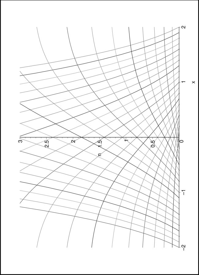
In Figure 5 x ( t , s ) , n ( t , s ) 𝑥 𝑡 𝑠 𝑛 𝑡 𝑠
x(t,s),n(t,s) s ∈ [ − 2..2 ] . 𝑠 delimited-[] 2..2 s\in\left[-2..2\right].
Figure 5: A plot of the rays x ( t , s ) , n ( t , s ) 𝑥 𝑡 𝑠 𝑛 𝑡 𝑠
x(t,s),n(t,s) s ∈ [ − 2..2 ] . 𝑠 delimited-[] 2..2 s\in\left[-2..2\right].
Using (51 47
d f d t 𝑑 𝑓 𝑑 𝑡 \displaystyle\frac{df}{dt} = π 2 s exp ( s 2 2 ) ( t + s ) [ erf ( t + s 2 ) − erf ( s 2 ) ] absent 𝜋 2 𝑠 superscript 𝑠 2 2 𝑡 𝑠 delimited-[] erf 𝑡 𝑠 2 erf 𝑠 2 \displaystyle=\sqrt{\frac{\pi}{2}}s\exp\left(\frac{s^{2}}{2}\right)\left(t+s\right)\left[\operatorname{erf}\left(\frac{t+s}{\sqrt{2}}\right)-\operatorname{erf}\left(\frac{s}{\sqrt{2}}\right)\right] (52)
+ s [ 1 + 1 2 t 2 + s t − ln ( s ) ] exp ( − 1 2 t 2 − s t ) − ( t + s ) . 𝑠 delimited-[] 1 1 2 superscript 𝑡 2 𝑠 𝑡 𝑠 1 2 superscript 𝑡 2 𝑠 𝑡 𝑡 𝑠 \displaystyle+s\left[1+\frac{1}{2}t^{2}+st-\ln\left(s\right)\right]\exp\left(-\frac{1}{2}t^{2}-st\right)-\left(t+s\right).
Using (49 44
f ( 0 , s ) = f 0 , 𝑓 0 𝑠 subscript 𝑓 0 f(0,s)=f_{0}, (53)
and solving (52 53
f ( t , s ) 𝑓 𝑡 𝑠 \displaystyle f(t,s) = π 2 exp ( s 2 2 ) [ erf ( t + s 2 ) − erf ( s 2 ) ] absent 𝜋 2 superscript 𝑠 2 2 delimited-[] erf 𝑡 𝑠 2 erf 𝑠 2 \displaystyle=\sqrt{\frac{\pi}{2}}\exp\left(\frac{s^{2}}{2}\right)\left[\operatorname{erf}\left(\frac{t+s}{\sqrt{2}}\right)-\operatorname{erf}\left(\frac{s}{\sqrt{2}}\right)\right] (54)
× s [ 1 + 1 2 t 2 + s t − ln ( s ) ] − ( 1 2 t 2 + s t ) + f 0 absent 𝑠 delimited-[] 1 1 2 superscript 𝑡 2 𝑠 𝑡 𝑠 1 2 superscript 𝑡 2 𝑠 𝑡 subscript 𝑓 0 \displaystyle\times s\left[1+\frac{1}{2}t^{2}+st-\ln\left(s\right)\right]-\left(\frac{1}{2}t^{2}+st\right)+f_{0}
or, using (5
f = [ ln ( s ) − 1 ] n + 1 2 ( s 2 − x 2 ) ( n + 1 ) + f 0 . 𝑓 delimited-[] 𝑠 1 𝑛 1 2 superscript 𝑠 2 superscript 𝑥 2 𝑛 1 subscript 𝑓 0 f=\left[\ln\left(s\right)-1\right]n+\frac{1}{2}\left(s^{2}-x^{2}\right)\left(n+1\right)+f_{0}. (55)
To solve the transport equation (42 ∂ 2 f ∂ n 2 , ∂ g ∂ n superscript 2 𝑓 superscript 𝑛 2 𝑔 𝑛
\frac{\partial^{2}f}{\partial n^{2}},\frac{\partial g}{\partial n} ∂ g ∂ x 𝑔 𝑥 \frac{\partial g}{\partial x} t 𝑡 t s . 𝑠 s.
[ ∂ x ∂ t ∂ x ∂ s ∂ n ∂ t ∂ n ∂ s ] [ ∂ t ∂ x ∂ t ∂ n ∂ s ∂ x ∂ s ∂ n ] = [ 1 0 0 1 ] matrix 𝑥 𝑡 𝑥 𝑠 𝑛 𝑡 𝑛 𝑠 matrix 𝑡 𝑥 𝑡 𝑛 𝑠 𝑥 𝑠 𝑛 matrix 1 0 0 1 \begin{bmatrix}\frac{\partial x}{\partial t}&\frac{\partial x}{\partial s}\\
\frac{\partial n}{\partial t}&\frac{\partial n}{\partial s}\end{bmatrix}\begin{bmatrix}\frac{\partial t}{\partial x}&\frac{\partial t}{\partial n}\\
\frac{\partial s}{\partial x}&\frac{\partial s}{\partial n}\end{bmatrix}=\begin{bmatrix}1&0\\
0&1\end{bmatrix}
and hence,
[ ∂ t ∂ x ∂ t ∂ n ∂ s ∂ x ∂ s ∂ n ] = 1 J ( t , s ) [ ∂ n ∂ s − ∂ x ∂ s − ∂ n ∂ t ∂ x ∂ t ] , matrix 𝑡 𝑥 𝑡 𝑛 𝑠 𝑥 𝑠 𝑛 1 𝐽 𝑡 𝑠 matrix 𝑛 𝑠 𝑥 𝑠 𝑛 𝑡 𝑥 𝑡 \begin{bmatrix}\frac{\partial t}{\partial x}&\frac{\partial t}{\partial n}\\
\frac{\partial s}{\partial x}&\frac{\partial s}{\partial n}\end{bmatrix}=\frac{1}{J(t,s)}\begin{bmatrix}\frac{\partial n}{\partial s}&-\frac{\partial x}{\partial s}\\
-\frac{\partial n}{\partial t}&\frac{\partial x}{\partial t}\end{bmatrix}, (56)
where the Jacobian J ( t , s ) 𝐽 𝑡 𝑠 J(t,s)
J ( t , s ) = ∂ x ∂ t ∂ n ∂ s − ∂ x ∂ s ∂ n ∂ t = ∂ n ∂ s − ∂ n ∂ t . 𝐽 𝑡 𝑠 𝑥 𝑡 𝑛 𝑠 𝑥 𝑠 𝑛 𝑡 𝑛 𝑠 𝑛 𝑡 J\left(t,s\right)=\frac{\partial x}{\partial t}\frac{\partial n}{\partial s}-\frac{\partial x}{\partial s}\frac{\partial n}{\partial t}=\frac{\partial n}{\partial s}-\frac{\partial n}{\partial t}. (57)
Using (5
J = ( s + 1 s ) n + s . 𝐽 𝑠 1 𝑠 𝑛 𝑠 J=\left(s+\frac{1}{s}\right)n+s. (58)
Using q = ∂ f ∂ n 𝑞 𝑓 𝑛 q=\frac{\partial f}{\partial n} 42
1 2 ∂ q ∂ n + ∂ g ∂ n − ∂ g ∂ x e − q = 0 1 2 𝑞 𝑛 𝑔 𝑛 𝑔 𝑥 superscript 𝑒 𝑞 0 \frac{1}{2}\frac{\partial q}{\partial n}+\frac{\partial g}{\partial n}-\frac{\partial g}{\partial x}e^{-q}=0
or
∂ ∂ n ( 1 2 e q ) = ∂ g ∂ x − ∂ g ∂ n e q 𝑛 1 2 superscript 𝑒 𝑞 𝑔 𝑥 𝑔 𝑛 superscript 𝑒 𝑞 \frac{\partial}{\partial n}\left(\frac{1}{2}e^{q}\right)=\frac{\partial g}{\partial x}-\frac{\partial g}{\partial n}e^{q}
and using (46
∂ ∂ n ( 1 2 e q ) = ∂ g ∂ x ∂ x ∂ t + ∂ g ∂ n ∂ n ∂ t = ∂ g ∂ t . 𝑛 1 2 superscript 𝑒 𝑞 𝑔 𝑥 𝑥 𝑡 𝑔 𝑛 𝑛 𝑡 𝑔 𝑡 \frac{\partial}{\partial n}\left(\frac{1}{2}e^{q}\right)=\frac{\partial g}{\partial x}\frac{\partial x}{\partial t}+\frac{\partial g}{\partial n}\frac{\partial n}{\partial t}=\frac{\partial g}{\partial t}.
Since − e q = ∂ n ∂ t , superscript 𝑒 𝑞 𝑛 𝑡 -e^{q}=\frac{\partial n}{\partial t},
∂ ∂ n ( 1 2 e q ) = − 1 2 ∂ ∂ n ( ∂ n ∂ t ) = − 1 2 ( ∂ 2 n ∂ t 2 ∂ t ∂ n + ∂ 2 n ∂ t ∂ s ∂ s ∂ n ) 𝑛 1 2 superscript 𝑒 𝑞 1 2 𝑛 𝑛 𝑡 1 2 superscript 2 𝑛 superscript 𝑡 2 𝑡 𝑛 superscript 2 𝑛 𝑡 𝑠 𝑠 𝑛 \displaystyle\frac{\partial}{\partial n}\left(\frac{1}{2}e^{q}\right)=-\frac{1}{2}\frac{\partial}{\partial n}\left(\frac{\partial n}{\partial t}\right)=-\frac{1}{2}\left(\frac{\partial^{2}n}{\partial t^{2}}\frac{\partial t}{\partial n}+\frac{\partial^{2}n}{\partial t\partial s}\frac{\partial s}{\partial n}\right)
= − 1 2 J ( − ∂ 2 n ∂ t 2 ∂ x ∂ s + ∂ 2 n ∂ t ∂ s ∂ x ∂ t ) = − 1 2 J ( − ∂ 2 n ∂ t 2 + ∂ 2 n ∂ t ∂ s ) absent 1 2 𝐽 superscript 2 𝑛 superscript 𝑡 2 𝑥 𝑠 superscript 2 𝑛 𝑡 𝑠 𝑥 𝑡 1 2 𝐽 superscript 2 𝑛 superscript 𝑡 2 superscript 2 𝑛 𝑡 𝑠 \displaystyle=-\frac{1}{2J}\left(-\frac{\partial^{2}n}{\partial t^{2}}\frac{\partial x}{\partial s}+\frac{\partial^{2}n}{\partial t\partial s}\frac{\partial x}{\partial t}\right)=-\frac{1}{2J}\left(-\frac{\partial^{2}n}{\partial t^{2}}+\frac{\partial^{2}n}{\partial t\partial s}\right)
= − 1 2 J ∂ ∂ t ( ∂ n ∂ s − ∂ n ∂ t ) = − 1 2 J ∂ J ∂ t , absent 1 2 𝐽 𝑡 𝑛 𝑠 𝑛 𝑡 1 2 𝐽 𝐽 𝑡 \displaystyle=-\frac{1}{2J}\frac{\partial}{\partial t}\left(\frac{\partial n}{\partial s}-\frac{\partial n}{\partial t}\right)=-\frac{1}{2J}\frac{\partial J}{\partial t},
where we have used (56 57
∂ g ∂ t = − 1 2 J ∂ J ∂ t 𝑔 𝑡 1 2 𝐽 𝐽 𝑡 \frac{\partial g}{\partial t}=-\frac{1}{2J}\frac{\partial J}{\partial t}
and therefore
g ( t , s ) = − 1 2 ln ( J ) + C ( s ) 𝑔 𝑡 𝑠 1 2 𝐽 𝐶 𝑠 g(t,s)=-\frac{1}{2}\ln(J)+C(s)
for some function C ( s ) . 𝐶 𝑠 C(s). 39 g ( 0 , s ) = 0 , 𝑔 0 𝑠 0 g(0,s)=0, 58 J ( 0 , s ) = s , 𝐽 0 𝑠 𝑠 J(0,s)=s, C ( s ) = 1 2 ln ( s ) 𝐶 𝑠 1 2 𝑠 C(s)=\frac{1}{2}\ln(s)
g ( t , s ) = 1 2 ln [ s J ( t , s ) ] . 𝑔 𝑡 𝑠 1 2 𝑠 𝐽 𝑡 𝑠 g(t,s)=\frac{1}{2}\ln\left[\frac{s}{J(t,s)}\right]. (59)
Using (58 59
g = 1 2 ln [ s 2 ( n + 1 ) s 2 + n ] . 𝑔 1 2 superscript 𝑠 2 𝑛 1 superscript 𝑠 2 𝑛 g=\frac{1}{2}\ln\left[\frac{s^{2}}{\left(n+1\right)s^{2}+n}\right]. (60)
Replacing f 𝑓 f g 𝑔 g 38 55 60 P n ( x ) ∼ Φ ( x , n ; s ) similar-to subscript 𝑃 𝑛 𝑥 Φ 𝑥 𝑛 𝑠 P_{n}(x)\sim\Phi\left(x,n;s\right) n → ∞ , → 𝑛 n\rightarrow\infty,
Φ ( x , n ; s ) = κ exp [ 1 2 ( s 2 − x 2 ) ( n + 1 ) − n ] s n n + 1 + n s − 2 , Φ 𝑥 𝑛 𝑠 𝜅 1 2 superscript 𝑠 2 superscript 𝑥 2 𝑛 1 𝑛 superscript 𝑠 𝑛 𝑛 1 𝑛 superscript 𝑠 2 \Phi\left(x,n;s\right)=\kappa\exp\left[\frac{1}{2}\left(s^{2}-x^{2}\right)\left(n+1\right)-n\right]\frac{s^{n}}{\sqrt{n+1+ns^{-2}}}, (61)
where κ = e f 0 𝜅 superscript 𝑒 subscript 𝑓 0 \kappa=e^{f_{0}}
Eliminating t 𝑡 t 5
n + π 2 s exp ( s 2 2 ) [ erf ( x 2 ) − erf ( s 2 ) ] = 0 , 𝑛 𝜋 2 𝑠 superscript 𝑠 2 2 delimited-[] erf 𝑥 2 erf 𝑠 2 0 n+\sqrt{\frac{\pi}{2}}s\exp\left(\frac{s^{2}}{2}\right)\left[\operatorname{erf}\left(\frac{x}{\sqrt{2}}\right)-\operatorname{erf}\left(\frac{s}{\sqrt{2}}\right)\right]=0, (62)
which defines s ( x , n ) 𝑠 𝑥 𝑛 s(x,n) n > 0 𝑛 0 n>0 S m ( x , n ) < 0 subscript 𝑆 𝑚 𝑥 𝑛 0 S_{m}(x,n)<0 S p ( x , n ) > 0 subscript 𝑆 𝑝 𝑥 𝑛 0 S_{p}(x,n)>0 62 erf ( x ) erf 𝑥 \operatorname{erf}(x)
S m ( x , n ) = − S p ( − x , n ) . subscript 𝑆 𝑚 𝑥 𝑛 subscript 𝑆 𝑝 𝑥 𝑛 S_{m}(x,n)=-S_{p}(-x,n). (63)
Although we have P n ( x ) ∼ Φ [ x , n ; S m ( x , n ) ] similar-to subscript 𝑃 𝑛 𝑥 Φ 𝑥 𝑛 subscript 𝑆 𝑚 𝑥 𝑛
P_{n}(x)\sim\Phi\left[x,n;S_{m}(x,n)\right] x ≪ − 1 much-less-than 𝑥 1 x\ll-1 P n ( x ) ∼ Φ [ x , n ; S p ( x , n ) ] similar-to subscript 𝑃 𝑛 𝑥 Φ 𝑥 𝑛 subscript 𝑆 𝑝 𝑥 𝑛
P_{n}(x)\sim\Phi\left[x,n;S_{p}(x,n)\right] x ≫ 1 , much-greater-than 𝑥 1 x\gg 1, x 𝑥 x
We shall now find the constant κ 𝜅 \kappa 61 7 62
s 2 exp ( s 2 ) = n 2 [ ∫ s x exp ( − θ 2 2 ) 𝑑 θ ] − 2 superscript 𝑠 2 superscript 𝑠 2 superscript 𝑛 2 superscript delimited-[] superscript subscript 𝑠 𝑥 superscript 𝜃 2 2 differential-d 𝜃 2 s^{2}\exp\left(s^{2}\right)=n^{2}\left[\int\limits_{s}^{x}\exp\left(-\frac{\theta^{2}}{2}\right)d\theta\right]^{-2} (64)
and for a fixed value of n , 𝑛 n, x → ∞ . → 𝑥 x\rightarrow\infty. 64 S p ( x , n ) ∼ x similar-to subscript 𝑆 𝑝 𝑥 𝑛 𝑥 S_{p}(x,n)\sim x
S p ( x , n ) ∼ x + s 0 + s 1 x − 1 + s 2 x − 2 + s 3 x − 3 , x → ∞ . formulae-sequence similar-to subscript 𝑆 𝑝 𝑥 𝑛 𝑥 subscript 𝑠 0 subscript 𝑠 1 superscript 𝑥 1 subscript 𝑠 2 superscript 𝑥 2 subscript 𝑠 3 superscript 𝑥 3 → 𝑥 S_{p}(x,n)\sim x+s_{0}+s_{1}x^{-1}+s_{2}x^{-2}+s_{3}x^{-3},\quad x\rightarrow\infty. (65)
Using (65 64
s 0 subscript 𝑠 0 \displaystyle s_{0} = s 2 = 0 , s 1 = ln ( n + 1 ) , formulae-sequence absent subscript 𝑠 2 0 subscript 𝑠 1 𝑛 1 \displaystyle=s_{2}=0,\quad s_{1}=\ln\left(n+1\right),
s 3 subscript 𝑠 3 \displaystyle\quad s_{3} = 1 − ln ( n + 1 ) − ln 2 ( n + 1 ) 2 − 1 n + 1 absent 1 𝑛 1 superscript 2 𝑛 1 2 1 𝑛 1 \displaystyle=1-\ln\left(n+1\right)-\frac{\ln^{2}\left(n+1\right)}{2}-\frac{1}{n+1}
and therefore
s 2 exp ( s 2 ) ∼ ( n + 1 ) 2 x 2 e x 2 , x → ∞ . formulae-sequence similar-to superscript 𝑠 2 superscript 𝑠 2 superscript 𝑛 1 2 superscript 𝑥 2 superscript 𝑒 superscript 𝑥 2 → 𝑥 s^{2}\exp\left(s^{2}\right)\sim\left(n+1\right)^{2}x^{2}e^{x^{2}},\quad x\rightarrow\infty. (66)
Solving (66
S p ( x , n ) ∼ W [ ( n + 1 ) 2 x 2 e x 2 ] , x → ∞ , formulae-sequence similar-to subscript 𝑆 𝑝 𝑥 𝑛 W superscript 𝑛 1 2 superscript 𝑥 2 superscript 𝑒 superscript 𝑥 2 → 𝑥 S_{p}(x,n)\sim\sqrt{\operatorname*{W}\left[\left(n+1\right)^{2}x^{2}e^{x^{2}}\right]},\quad x\rightarrow\infty, (67)
where W ( z ) W 𝑧 \operatorname*{W}\left(z\right) [3 ]
W ( z ) exp [ W ( z ) ] = z , ∀ z ∈ ℂ formulae-sequence W 𝑧 W 𝑧 𝑧 for-all 𝑧 ℂ \operatorname*{W}\left(z\right)\exp\left[\operatorname*{W}\left(z\right)\right]=z,\quad\forall z\in\mathbb{C}
and having the asymptotic behavior
W ( z ) = ln ( z ) − ln ln ( z ) + ln ln ( z ) ln ( z ) + O ( [ ln ln ( z ) ln ( z ) ] 2 ) , z → ∞ . formulae-sequence W 𝑧 𝑧 𝑧 𝑧 𝑧 𝑂 superscript delimited-[] 𝑧 𝑧 2 → 𝑧 \operatorname*{W}\left(z\right)=\ln(z)-\ln\ln\left(z\right)+\frac{\ln\ln(z)}{\ln(z)}+O\left(\left[\frac{\ln\ln(z)}{\ln(z)}\right]^{2}\right),\quad z\rightarrow\infty. (68)
Using (67 68 61
Φ ( x , n ; s ) ∼ κ ( n + 1 ) n + 1 2 e − n x n , x → ∞ . formulae-sequence similar-to Φ 𝑥 𝑛 𝑠 𝜅 superscript 𝑛 1 𝑛 1 2 superscript 𝑒 𝑛 superscript 𝑥 𝑛 → 𝑥 \Phi\left(x,n;s\right)\sim\kappa\left(n+1\right)^{n+\frac{1}{2}}e^{-n}x^{n},\quad x\rightarrow\infty.
From Stirling’s formula
n ! = [ 2 π n + O ( n − 1 2 ) ] n n e − n , n → ∞ , formulae-sequence 𝑛 delimited-[] 2 𝜋 𝑛 𝑂 superscript 𝑛 1 2 superscript 𝑛 𝑛 superscript 𝑒 𝑛 → 𝑛 n!=\left[\sqrt{2\pi n}+O\left(n^{-\frac{1}{2}}\right)\right]n^{n}e^{-n},\quad n\rightarrow\infty, (69)
and
( n + 1 ) n + 1 2 = [ e n + O ( n − 1 2 ) ] n n , n → ∞ , formulae-sequence superscript 𝑛 1 𝑛 1 2 delimited-[] 𝑒 𝑛 𝑂 superscript 𝑛 1 2 superscript 𝑛 𝑛 → 𝑛 \left(n+1\right)^{n+\frac{1}{2}}=\left[e\sqrt{n}+O\left(n^{-\frac{1}{2}}\right)\right]n^{n},\quad n\rightarrow\infty,
we conclude that
κ = e − 1 2 π 𝜅 superscript 𝑒 1 2 𝜋 \kappa=e^{-1}\sqrt{2\pi}
and thus
Φ ( x , n ; s ) = s n exp [ 1 2 ( s 2 − x 2 − 2 ) ( n + 1 ) ] 2 π s 2 ( n + 1 ) s 2 + n . Φ 𝑥 𝑛 𝑠 superscript 𝑠 𝑛 1 2 superscript 𝑠 2 superscript 𝑥 2 2 𝑛 1 2 𝜋 superscript 𝑠 2 𝑛 1 superscript 𝑠 2 𝑛 \Phi\left(x,n;s\right)=s^{n}\exp\left[\frac{1}{2}\left(s^{2}-x^{2}-2\right)\left(n+1\right)\right]\sqrt{\frac{2\pi s^{2}}{\left(n+1\right)s^{2}+n}}. (70)
Using (63 P n ( x ) ∼ Ψ 4 ( x , n ) similar-to subscript 𝑃 𝑛 𝑥 subscript Ψ 4 𝑥 𝑛 P_{n}(x)\sim\Psi_{4}(x,n) n → ∞ , → 𝑛 n\rightarrow\infty,
Ψ 4 ( x , n ) = Φ [ x , n ; S p ( x , n ) ] + Φ [ x , n ; − S p ( − x , n ) ] , n → ∞ . formulae-sequence subscript Ψ 4 𝑥 𝑛 Φ 𝑥 𝑛 subscript 𝑆 𝑝 𝑥 𝑛
Φ 𝑥 𝑛 subscript 𝑆 𝑝 𝑥 𝑛
→ 𝑛 \Psi_{4}(x,n)=\Phi\left[x,n;S_{p}(x,n)\right]+\Phi\left[x,n;-S_{p}(-x,n)\right],\quad n\rightarrow\infty. (71)
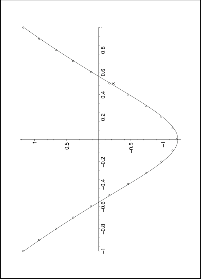
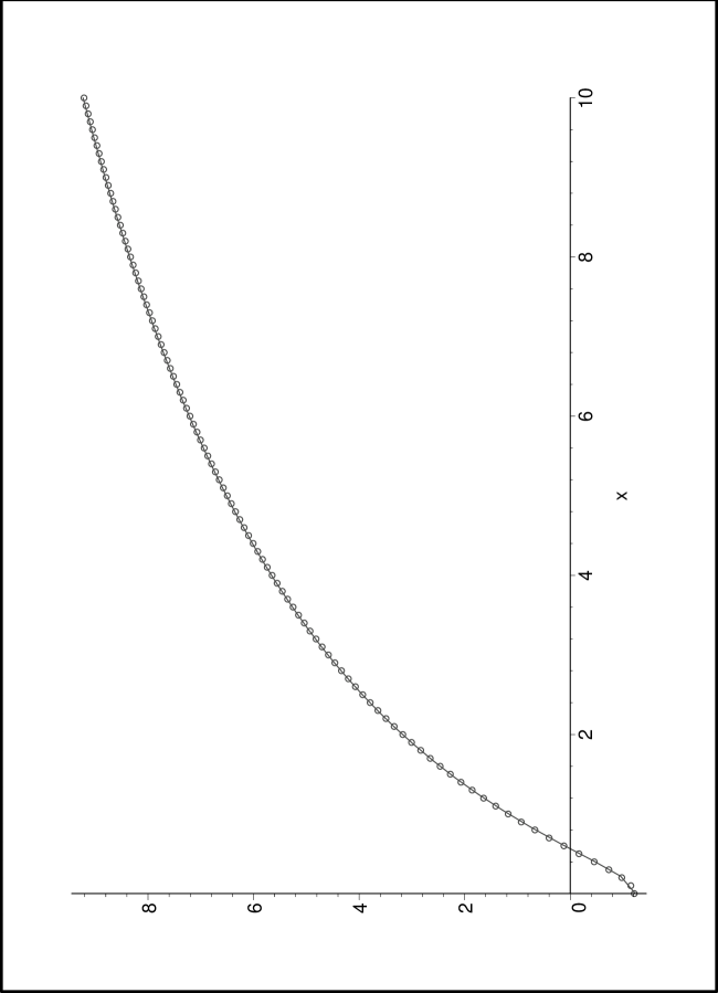
In Figure 6 ln [ P 4 ( x ) / 4 ! ] subscript 𝑃 4 𝑥 4 \ln\left[P_{4}(x)/4!\right] ln [ Ψ 4 ( x , 4 ) / 4 ! ] subscript Ψ 4 𝑥 4 4 \ln\left[\Psi_{4}(x,4)/4!\right] 0 < x < 10 0 𝑥 10 0<x<10 7 − 1 < x < 1 . 1 𝑥 1 -1<x<1. 71 14 18 20 S p ( x , n ) subscript 𝑆 𝑝 𝑥 𝑛 S_{p}(x,n)
Figure 6: A plot of ln [ P 4 ( x ) / 4 ! ] subscript 𝑃 4 𝑥 4 \ln\left[P_{4}(x)/4!\right] ln [ Ψ 4 ( x , 4 ) / 4 ! ] subscript Ψ 4 𝑥 4 4 \ln\left[\Psi_{4}(x,4)/4!\right]
Figure 7: A plot of ln [ P 4 ( x ) / 4 ! ] subscript 𝑃 4 𝑥 4 \ln\left[P_{4}(x)/4!\right] ln [ Ψ 4 ( x , 4 ) / 4 ! ] subscript Ψ 4 𝑥 4 4 \ln\left[\Psi_{4}(x,4)/4!\right]
Next, we compare the results of this section with those in the previous two
sections. We first consider x > 0 , 𝑥 0 x>0, x = O ( 1 ) 𝑥 𝑂 1 x=O(1) n → ∞ . → 𝑛 n\rightarrow\infty. 62
S p ( x , n ) ∼ W [ ( n + 1 ) 2 ζ 2 ( x ) ] , similar-to subscript 𝑆 𝑝 𝑥 𝑛 W superscript 𝑛 1 2 superscript 𝜁 2 𝑥 S_{p}(x,n)\sim\sqrt{\operatorname*{W}\left[\frac{\left(n+1\right)^{2}}{\zeta^{2}(x)}\right]}, (72)
where ζ ( x ) 𝜁 𝑥 \zeta(x) 15 72 68 70
P n ( x ) ∼ n n e − n n π ln ( n ) [ e − x 2 / 2 ζ ( x ) ] n + 1 , similar-to subscript 𝑃 𝑛 𝑥 superscript 𝑛 𝑛 superscript 𝑒 𝑛 𝑛 𝜋 𝑛 superscript delimited-[] superscript 𝑒 superscript 𝑥 2 2 𝜁 𝑥 𝑛 1 P_{n}(x)\sim n^{n}e^{-n}\sqrt{\frac{n\pi}{\ln\left(n\right)}}\left[\frac{e^{-x^{2}/2}}{\zeta(x)}\right]^{n+1},
which agrees with (14 69
Now we consider the limit n → ∞ , → 𝑛 n\rightarrow\infty, x = y / n 𝑥 𝑦 𝑛 x=y/n y = O ( 1 ) . 𝑦 𝑂 1 y=O(1). 62
S p ( y / n , n ) ∼ W ( 2 n 2 π ) + ( 1 + 2 π y ) 1 W ( 2 n 2 π ) n . similar-to subscript 𝑆 𝑝 𝑦 𝑛 𝑛 W 2 superscript 𝑛 2 𝜋 1 2 𝜋 𝑦 1 W 2 superscript 𝑛 2 𝜋 𝑛 S_{p}\left(y/n,n\right)\sim\sqrt{\operatorname*{W}\left(\frac{2n^{2}}{\pi}\right)}+\left(1+\sqrt{\frac{2}{\pi}}y\right)\frac{1}{\sqrt{\operatorname*{W}\left(\frac{2n^{2}}{\pi}\right)}n}. (73)
Using (73 63 68 70
Φ ( y / n , n ; S p ) Φ 𝑦 𝑛 𝑛 subscript 𝑆 𝑝 \displaystyle\Phi\left(y/n,n;S_{p}\right) ∼ n n e − n 2 n ln ( n ) ( 2 π ) n exp ( 2 π y ) , similar-to absent superscript 𝑛 𝑛 superscript 𝑒 𝑛 2 𝑛 𝑛 superscript 2 𝜋 𝑛 2 𝜋 𝑦 \displaystyle\sim n^{n}e^{-n}\sqrt{\frac{2n}{\ln(n)}}\left(\sqrt{\frac{2}{\pi}}\right)^{n}\exp\left(\sqrt{\frac{2}{\pi}}y\right),
Φ ( y / n , n ; S m ) Φ 𝑦 𝑛 𝑛 subscript 𝑆 𝑚 \displaystyle\Phi\left(y/n,n;S_{m}\right) ∼ ( − 1 ) n n n e − n 2 n ln ( n ) ( 2 π ) n exp ( − 2 π y ) similar-to absent superscript 1 𝑛 superscript 𝑛 𝑛 superscript 𝑒 𝑛 2 𝑛 𝑛 superscript 2 𝜋 𝑛 2 𝜋 𝑦 \displaystyle\sim\left(-1\right)^{n}n^{n}e^{-n}\sqrt{\frac{2n}{\ln(n)}}\left(\sqrt{\frac{2}{\pi}}\right)^{n}\exp\left(-\sqrt{\frac{2}{\pi}}y\right)
and therefore
P n ( x ) ∼ n n e − n 2 n ln ( n ) ( 2 π ) n [ exp ( 2 π y ) + ( − 1 ) n exp ( − 2 π y ) ] similar-to subscript 𝑃 𝑛 𝑥 superscript 𝑛 𝑛 superscript 𝑒 𝑛 2 𝑛 𝑛 superscript 2 𝜋 𝑛 delimited-[] 2 𝜋 𝑦 superscript 1 𝑛 2 𝜋 𝑦 P_{n}(x)\sim n^{n}e^{-n}\sqrt{\frac{2n}{\ln(n)}}\left(\sqrt{\frac{2}{\pi}}\right)^{n}\left[\exp\left(\sqrt{\frac{2}{\pi}}y\right)+\left(-1\right)^{n}\exp\left(-\sqrt{\frac{2}{\pi}}y\right)\right]
agreeing with (18
Finally, we consider the limit n → ∞ → 𝑛 n\rightarrow\infty x = u ln ( n ) , 𝑥 𝑢 𝑛 x=u\sqrt{\ln\left(n\right)}, u = O ( 1 ) , 𝑢 𝑂 1 u=O(1), u > 0 . 𝑢 0 u>0. 62
S p ( u ln ( n ) , n ) ∼ W [ ( n + 1 ) 2 u 2 n u 2 ln ( n ) ] . similar-to subscript 𝑆 𝑝 𝑢 𝑛 𝑛 W superscript 𝑛 1 2 superscript 𝑢 2 superscript 𝑛 superscript 𝑢 2 𝑛 S_{p}\left(u\sqrt{\ln\left(n\right)},n\right)\sim\sqrt{\operatorname*{W}\left[\left(n+1\right)^{2}u^{2}n^{u^{2}}\ln(n)\right]}. (74)
Using (74 68 70
P n ( u ln ( n ) ) ∼ n n e − n 2 π n u n + 1 u 2 + 2 ( ln ( n ) ) n , n → ∞ , formulae-sequence similar-to subscript 𝑃 𝑛 𝑢 𝑛 superscript 𝑛 𝑛 superscript 𝑒 𝑛 2 𝜋 𝑛 superscript 𝑢 𝑛 1 superscript 𝑢 2 2 superscript 𝑛 𝑛 → 𝑛 P_{n}\left(u\sqrt{\ln\left(n\right)}\right)\sim n^{n}e^{-n}\sqrt{2\pi n}\frac{u^{n+1}}{\sqrt{u^{2}+2}}\left(\sqrt{\ln\left(n\right)}\right)^{n},\quad n\rightarrow\infty,
which agrees with (20
Acknowledgement 1
The work of D. Dominici was supported by a Humboldt Research Fellowship for
Experienced Researchers from the Alexander von Humboldt Foundation.
The work of C. Knessl was supported by the grants NSF 05-03745 and NSA H 98230-08-1-0102.