Primordial non-Gaussianities in the Intergalactic Medium

Abstract

We present results from the first high-resolution hydrodynamical simulations of non-Gaussian cosmological models. We focus on the statistical properties of the transmitted Lyman-$\alpha$ flux in the high redshift intergalactic medium. Imprints of non-Gaussianity are present and are larger at high redshifts. Differences larger than 20% at $z>3$ in the flux probability distribution function for high transmissivity regions (voids) are expected for values of the non linearity parameter $f_{\rm NL}=\pm 100$ when compared to a standard $\Lambda$CDM cosmology with $f_{\rm NL}=0$. We investigate also the one-dimensional flux bispectrum: at the largest scales (corresponding to tens of Mpc) we expect deviations in the flux bispectrum up to 20% at $z\sim 4$ (for $f_{\rm NL}=\pm 100$), significantly larger than deviations of $\sim 3\%$ in the flux power spectrum. We briefly discuss possible systematic errors that can contaminate the signal. Although challenging, a detection of non-Gaussianities in the interesting regime of scales and redshifts probed by the Lyman-$\alpha$ forest, could be possible with future data sets.

1 Introduction

According to the standard gravitational instability picture present-day cosmic structures have evolved from tiny initial fluctuations in the mass density field that obey Gaussian statistics. However, departures from Gaussianity inevitably arise at some level during the inflationary epoch. The various mechanisms that produce primordial non-Gaussianity during inflation have been thoroughly investigated by Bartolo et al. (2004) (and references therein). A convenient way of modeling non-Gaussianity is to include quadratic correction in the Bardeen’s gauge-invariant potential $\Phi$:

$$\Phi=\Phi_{\rm L}+f_{\rm{\rm NL}}\left(\Phi_{\rm L}^{2}-\langle\Phi_{\rm L}^{2}\rangle\right)\;,$$ (1)

where $\Phi_{\rm L}$ represents a Gaussian random field and the dimensionless parameter $f_{\rm{\rm NL}}$ quantifies the amplitude of the corrections to the curvature perturbations. The above definition in which the term $-f_{\rm{\rm NL}}\,\langle\Phi_{\rm L}^{2}\rangle$ is small guarantees that $<\Phi>=<\Phi_{\rm L}>=0$. Although the quadratic model quantifies the level of primordial non-Gaussianity predicted by a large number of scenarios for the generation of the initial seeds for structure formation (including standard single-field and multi-field inflation, the curvaton and the inhomogeneous reheating scenarios), one should keep in mind that there are different ways for a density field to be non-Gaussian (NG) and that different observational tests capable of going beyond second order statistics should be used to fully characterize the nature of non-Gaussianity.

To date, the strongest observational constraint for NG models are provided by the recent analysis of the WMAP 5-year temperature fluctuation maps (Komatsu et al., 2008) according to which $-9<f_{\rm NL}<111$ at the 95 % confidence level in the local model. The large scale structure (LSS) provides alternative observational constraints which are, in principle, more stringent than the cosmic microwave background (CMB) since they carry information on the 3D primordial fluctuation fields, rather than on a 2D temperature map. Moreover, if the level of primordial non-Gaussianity depends on scale then CMB and LSS provide independent constraints since they probe different scales. For this reason, the WMAP 5-year limits on $f_{\rm{\rm NL}}$ need not to apply on the smaller scales probed by the LSS and the NG models that we consider in this work, which have $|f_{\rm NL}|$ as large as 200, are thus not in conflict with the CMB on the scales which are relevant for our analysis.

A very promising way to constrain departures from Gaussianity is to measure the various properties of massive virialized structures like their abundance (Matarrese et al., 2000; Verde et al., 2001; Lo Verde et al., 2008), clustering and their biasing (Grinstein & Wise, 1986; Matarrese et al., 1986; Matarrese & Verde, 2008; Dalal et al., 2008; Carbone et al., 2008; Seljak, 2008; Matarrese & Verde, 2008). Indeed, the best constraints on non-Gaussianity from the LSS have been obtained by Slosar et al. (2008) including the observed scale-dependent bias of the spectroscopic sample SDSS luminous red galaxies and the photometric quasar sample. The resulting limits of $-29<f_{\rm NL}<70$ (95 % confidence level) are remarkably close to those obtained from the CMB analysis alone and, according to Seljak (2008), could be further improved by looking for scale dependency in the relative biasing of two different population of objects. Alternatively, one can consider the topology of the mass density field (Matsubara, 2003), and higher-order clustering statistics like the bispectrum (Hikage et al., 2006). The ability of these techniques to detect the imprint of the primordial non-Gaussianity on the LSS has been tested with N-body experiments (Messina et al., 1990; Moscardini et al., 1991; Weinberg & Cole, 1992; Mathis et al., 2004; Kang et al., 2007; Grossi et al., 2007; Dalal et al., 2008; Hikage et al., 2008). N-body simulations are of paramount importance in the study of NG models, since one needs to disentangle primordial non-Gaussianity from late non-Gaussianity induced by the non-linear growth of density perturbations that can only be properly accounted for by numerical experiments.

Recently, Grossi et al. (2007, 2008) have carried out cosmological N-body simulations of NG models to study the evolution of the probability distribution function (PDF) of the density fluctuations. They found that the imprint of primordial non-Gaussianity, which is evident in the negative tail of the PDF at high redshifts, is preserved throughout the subsequent evolution and out to the present epoch. This result suggests that void statistics may be a promising effective tool for detecting primordial non-Gaussianity (Kamionkowski et al. (2008); Song & Lee (2008)) and that can be applied to different types of observations over a large range of cosmic epochs. Taking advantage of the recent theoretical efforts for standardizing the appropriate statistical tools (Colberg, 2008) one could apply void-finding algorithms to quantify the properties of the underdense regions observed in the spatial distribution of galaxies. Unfortunately, current galaxy redshift surveys are probably too small for void-based statistics to appreciate deviations from the Gaussian case at the level required. The situation will change in a not too distant future, when next generation all-sky surveys like ADEPT or EUCLID will allow to measure the position of $\sim 5\times 10^{7}$ galaxies over a large range of redshifts out to $z=2$. Alternatively, one can analyze high-resolution spectra of distant quasars to characterize the properties of the underlying mass density field at $z>3$ (e.g. Viel et al. (2003); Viel et al. (2004); Viel et al. (2004b); Lesgourgues et al. (2007)). In particular, since we expect that underdense regions are characterized by a low neutral hydrogen (HI) abundance, one can infer the presence of voids and quantify their statistical properties from voids in the transmitted flux, defined as the connected regions in the spectral flux distribution above the mean flux level. The connection between voids and spectral regions characterized by negligible HI absorption has been recently studied by Viel et al. (2008) using hydrodynamical simulations where a link at $z\sim 2$ between the flux and matter properties is provided.

In this work we perform, for the first time, high-resolution hydrodynamical simulations of NG models to check whether one can use the intergalactic medium (see Meiksin (2007) for a recent review) to detect non-Gaussian features in the Lyman-$\alpha$ flux statistics like the PDF, flux power and the bispectrum. The layout of the paper is as follows. In Section  2 we describe the hydrodynamical simulations and we show an example of simulated Lyman-$\alpha$ quasar (QSO) spectrum. In Section  3 we present the results of the various flux statistics. In Section  4 we address the role of systematic and statistical errors that could contaminate the NG signal. We conclude in Section  5.

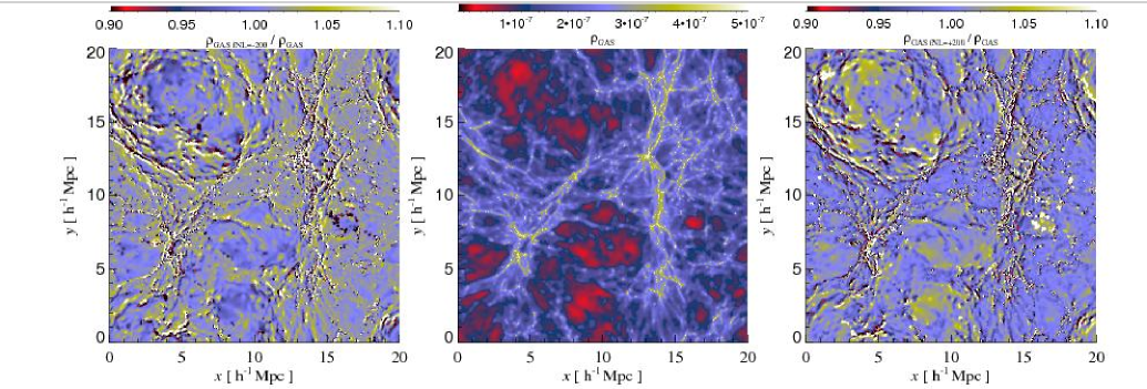
Figure 1: Gas (projected) density distribution in the hydrodynamical simulations at $z=3$ in the Gaussian case (middle panel) and residuals in the gas distribution for non-Gaussian models with $f_{\rm NL}=-200$ (left panel) and $f_{\rm NL}=+200$ (right panel). The simulated box has a linear size of 20 comoving Mpc$/h$ and the thickness of the slice shown is 1.5 comoving Mpc$/h$. The cosmic web that gives rise to Lyman-$\alpha$ absorption is visible and the tendency for regions below the mean density to be underdense (overdense) in models with negative (positive) values of $f_{\rm NL}$ is clear.

2 Non-Gaussian hydrodynamical simulations

We rely on simulations run with the parallel hydrodynamical (TreeSPH) code GADGET-2 based on the conservative ‘entropy-formulation’ of SPH (Springel, 2005). They consist of a cosmological volume with periodic boundary conditions filled with an equal number of dark matter and gas particles. Radiative cooling and heating processes were followed for a primordial mix of hydrogen and helium. We assumed a mean Ultraviolet Background similar to that propesed by Haardt & Madau (1996) produced by quasars and galaxies as given by with helium heating rates multiplied by a factor 3.3 in order to better fit observational constraints on the temperature evolution of the IGM (e.g. Schaye et al. (2000); Ricotti et al. (2000)). This background gives naturally a hydrogen ionization rate $\Gamma_{-12}\sim 1$ at the redshifts of interest here (e.g. Bolton et al. (2005); Faucher-Giguère et al. (2008)). The star formation criterion is a very simple one that converts in collisionless stars all the gas particles whose temperature falls below $10^{5}$ K and whose density contrast is larger than 1000 (it has been shown that the star formation criterion has a negligible impact on flux statistics). More details can be found in (Viel et al., 2004).

The cosmological reference model corresponds to a ‘fiducial’ $\Lambda$CDM Universe with parameters, at $z=0$, $\Omega_{\rm m}=0.26,\ \Omega_{\rm\Lambda}=0.74,\ \Omega_{\rm b}=0.0463$, $n_{\rm s}=0.95$, and $H_{0}=72$ km s^-1 Mpc^-1 and $\sigma_{8}=0.85$ (the B2 series of Viel et al. (2004)). We have used $2\times 384^{3}$ dark matter and gas particles in a $60\ h^{-1}$ comoving Mpc box for the flux power and bispectrum, to better sample the large scales. For the flux probability distribution function we relied instead on $2\times 256^{3}$ dark matter and gas particles in a $20\ h^{-1}$ comoving Mpc, since below and around $z=3$ this seems to be the appropriate resolution the get numerical convergence. The gravitational softening was set to 2.5 and 5 $h^{-1}$ kpc in comoving units for all particles for the 20 and 60 comoving Mpc/$h$ boxes, respectively. The mass per gas particle is $6.12\times 10^{6}$M${}_{\odot}/h$ for the small boxes and $4.9\times 10^{7}$M${}_{\odot}/h$ for the large boxes, while the high resolution run for the small box has a mass per gas particle of $1.8\times 10^{6}$M${}_{\odot}/h$ (this refers to a (20,384) simulation that was performed in order to check for numerical convergence of the flux PDF). In the following, the different simulations will be indicated by two numbers, $(N_{1},N_{2})$: $N_{1}$ is the size of the box in comoving Mpc$/h$ and $N_{2}$ is the cubic root of the total number of gas particles in the simulation. NG are produced in the initial conditions at $z=99$ using the same method as in Grossi et al. (2007) that we briefly summarize here. Initial NG conditions are generated without modifying the linear matter power spectrum using the Zel’dovich approximation: a Gaussian gravitational potential is generated in Fourier space from a power-law power spectrum of the form $P(k)\propto k^{-3}$ and inverse Fourier transformed in real space to produce $\phi_{\rm L}$. The final $\Phi$ is obtained using eq. (1). Finally, back in Fourier space, we modulate the power-law spectrum using the transfer functions of the $\Lambda$CDM model.

We also run some other simulations at higher resolutions to check for numerical convergence. In particular we have performed a $(20,384)$ simulation run to analyse the flux PDF. For the $(20,256)$ models the flux probability distribution function has numerically converged only below $z=3$ (see Bolton et al. (2008)). However, since our results will always be quoted in comparison with the $f_{\rm NL}=0$ case (i.e. as a ratio of two different quantities) we expect the resolution errors to be unimportant (i.e. we assume the same resolution corrections should be applied to all the models, even though this assumption should be explicitly checked).

A projected density slice of the gas (IGM) distribution for the (20,256) simulation of thickness 1.5 comoving Mpc/$h$ is shown in Figure 1. We focus on this simulation because at $z=3$ the flux probability distribution function has numerically converged. In the middle panel we plot the gas density in the Gaussian case, while residuals in the two models with $f_{\rm NL}=-200$ and f${}_{\rm NL}=+200$ are shown in the left and right panel, respectively. On average regions of the cosmic web below the mean density appear to be $\sim 10\%$ less (more) dense in the negative (positive) $f_{\rm NL}$ case. This trend is apparent not only near the centre of these regions but also in the matter surrounding them (see for example the void at $(x=17;y=8)$ comoving Mpc$/h$). The same qualitative behavior can be observed in the distribution of the dark matter particles (see Figure 2 of Grossi et al. (2008)).

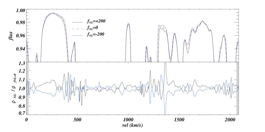
Figure 2: Simulated noiseless Lyman-$\alpha$ flux (only regions at high transmissivity are shown) at $z=3$ in the upper panel. Models with positive and negative values of $f_{\rm NL}$ bracket the Gaussian case with $f_{\rm NL}=0$. Although difficult to see on a pixel-by-pixel basis, differences among the models can be appreciated in a statistical sense when many spectra are considered (see text). The bottom panel shows the ratio of non-Gaussian models to the Gaussian one for the one-dimensional gas density along the line-of-sight (in real space). On average differences of the order 10% are present.

In the NG models considered here the growth of structures in terms of density PDF is different. As discussed in Grossi et al. (2008), the maps of residuals in the non-Gaussian cases reflect the differences in the primordial PDF of the mass overdensity. As shown in Figures 1 and 5 of Grossi et al. (2008) the mass PDF is skewed towards positive (negative) overdensities in the non-Gaussian models with positive (negative) $f_{\rm NL}$ values, compared to the Gaussian case. As a consequence, since the gas traces well the underlying mass distribution at these redshifts, voids look emptier in the $f_{\rm NL}=-200$ case (map on the left) while denser environments like filaments and knots look more prominent in the $f_{\rm NL}=+200$ case (map on the right) with respect to the Gaussian case. These differences in the tails of the density PDF also impact on the filaments at around the mean density that surround the voids. In fact the size of the voids is slightly different in the negative and positive NG models: for negative $f_{\rm NL}$ values the emptier voids grow in size faster than for the Gaussian case and even faster than for positive $f_{\rm NL}$ values, displacing the filaments at around the mean densities at different positions in the three cases and giving rise to the filamentary pattern of residuals of the panels.

To perform our analysis we have extracted several mock QSO absorption spectra from the simulation box. All spectra are drawn in redshift space taking into account the effect of the IGM peculiar velocities along the line-of-sight $v_{\rm pec,\parallel}$. Basically, the simulated flux at the redshift-space coordinate $u$ (in km/s) is $F(u)=\exp[-\tau(u)]$ with:

$$\tau(u)={\sigma_{0,\alpha}~{}c\over H(z)}\int_{-\infty}^{\infty}dx\,n_{\rm HI}(x)~{}{\cal G}\left[u-x-v_{pec,\parallel}^{\rm IGM}(x),\,b(x)\right]dx\;,$$ (2)

where $\sigma_{0,\alpha}=4.45\times 10^{-18}$ cm² is the hydrogen Lyman-$\alpha$ cross-section, $H(z)$ is the Hubble constant at redshift $z$, $x$ is the real-space coordinate (in km s^-1), $b=(2k_{B}T/mc^{2})^{1/2}$ is the velocity dispersion in units of $c$, ${\cal G}=(\sqrt{\pi}b)^{-1}\exp[-(u-y-v_{\rm pec,\parallel}^{\rm IGM}(y))^{2}/b^{2}]$ is the Gaussian profile that well approximates the Voigt profile in the regime considered here. The neutral hydrogen density in real-space, that enters the equation above, could be related to the underlying gas density by the following expression (e.g. Hui & Gnedin (1997); Schaye (2001)):

$$n_{\rm HI}({\bf x},z) \approx 10^{-5}~{}{\overline{n}}_{\rm IGM}(z)\left({\Omega_{0b}h^{2}\over 0.019}\right)\left({\Gamma_{-12}\over 0.5}\right)^{-1}\times$$ (3)

$$\left(T({\bf x},z)\over 10^{4}{\rm K}\right)^{-0.7}\left({1+z\over 4}\right)^{3}\left(1+\delta_{\rm IGM}({\bf x},z)\right)^{2}\;,$$

with $\Gamma_{-12}$ is the hydrogen photoionization rate in units of $s^{-1}$, $T$ is the IGM temperature, and $\overline{n}_{\rm IGM}(z)$ is the mean IGM density at that redshift. However, this equation is not explicitly used since the neutral hydrogen fraction is computed self-consistently for each gas particles during the simulation run. The integral in eq. (2) to obtain the Lyman-$\alpha$ optical depth along each simulated line-of-sight is thus performed using the relevant hydrodynamical quantities from the numerical simulations: $\delta_{\rm IGM},T,v_{\rm pec},n_{\rm HI}$. More details on how to extract a mock QSO spectrum from an hydrodynamical simulation using the SPH formalism can be found in Theuns et al. (1998).

An example of line-of-sight is shown in the top panel of Figure 2, while the bottom panel shows the ratio of the gas density along the line-of-sight of NG and Gaussian models (in real space) In the following we will focus on high transmissivity in which the transmitted flux is close to unity (upper panel). Three QSO spectra are shown with different line styles and correspond to the Gaussian case (dashed, red line), and to $f_{\rm NL}=\pm 200$ (solid black and solid blue, respectively). The transmitted flux (no noise is added in this case) is almost identical for the two NG models in magnitude but not in sign, as expected. One can better appreciate the differences among the models by looking at the gas density (bottom panel). On average differences are of the order 10%, even if in some cases they can rise above 30-40%. The fact that the corresponding variations in the flux are comparatively smaller (usually less than few percent) is somehow expected, since differences in the gas density are exponentially suppressed by the non-linear transformation between flux and matter (and by other non-linear effects as well). However, despite their small amplitude, the differences in the transmitted flux are large enough to be appreciated through appropriate statistical analyses of many independent lines-of-sight, as we will see in the following sections. Global statistics will be usually shown for samples of 1000 lines-of-sight extracted along random directions within the simulated volume.

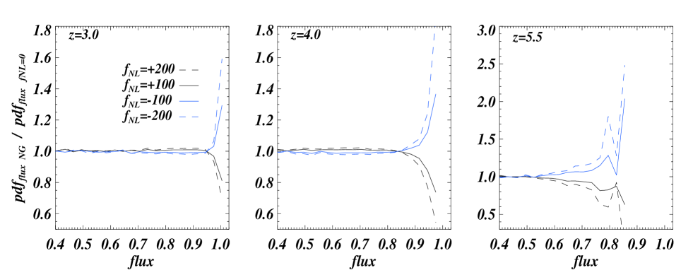
Figure 3: Ratio between the simulated flux probability distribution function of four different $(20,256)$ models with $f_{\rm NL}=-200,-100,+100,+200$ and $f_{\rm NL}=0$, represented by the blue dashed, blue continuous, black continuous and black dashed lines, respectively. Results are shown at $z=3,4,5.5$ in the left, middle and right panels. (Note the different scale in the right panel).

3 Results

3.1 The Lyman-$\alpha$ flux probability distribution function

In Figure 3 we show results for the flux probability distribution function at $z=3,4\ {\rm and}\ 5.5$ using the (20,256) simulations, in the left, middle and right panel, respectively. The mock QSO spectra have been normalized to reproduce the same (observed) mean flux level. The scaling factor is usually different by less than 2% to the standard non-Gaussian case (more precisely the differences are below 1% at z=3, around 1% at z=4.0 and around 2% at z=5.5 between the Gaussian and the $f_{\rm NL}=\pm 200$ cases). Differences between the non-Gaussian case and the Gaussian one are appreciable only in regions of high transmissivity (flux $\sim$ 1), that are typically associated to connected regions below mean density (voids) in the matter distribution. At $z=3$ (left panel) the differences can be of the order of 20% (40%) for models with $f_{\rm NL}=\pm\,100(\pm\,200)$. Models with negative (positive) values of $f_{\rm NL}$ produce less (more) absorption. This reflects the fact that voids in models with negative $f_{\rm NL}$ are emptier of neutral hydrogen than in the Gaussian case. The opposite holds true for models with positive $f_{\rm NL}$. This is analogous to the effect discussed by Grossi et al. (2008) on the dark matter density field and characterized in terms of the probability distribution function of density fluctuations. In that case for negative values of $f_{\rm NL}$ the low density tail of the dark matter density PDF is more prominent. In our case what is more prominent is the high flux tail of the Lyman-$\alpha$ flux PDF. The amplitude of the effect increases with the redshift. At $z=4$ (middle panel) differences w.r.t. the Gaussian case are as large as 30 %-60 % (for $f_{\rm NL}=\pm 100$ and $\pm 200$, respectively) and at $z=5.5$ (right panel) the differences are of the order of $\sim 100\,\%-150\%$ (for $f_{\rm NL}=\pm 100$ and $\pm 200$, respectively). Note that in the latter ($z=5.5$) case we have used a different scale for the $y-$axis.

From an observational viewpoint, it should be noted that the Lyman-$\alpha$ flux PDF has been measured with great accuracy using high-resolution spectra taking into account the metal contaminations and continuum fitting errors at $z=2.07,2.54,2.94$ by Kim et al. (2007). On the contrary, continuum fitting errors and the metal contaminations are somewhat harder to estimate in the measurements at higher redshifts ($z=4.5$ and $z=5.5$) by Becker et al. (2007). We will come back to this point in Section 4.

3.2 The Lyman-$\alpha$ flux void distribution function

A different, although not completely unrelated statistics is represented by the probability distribution function of the voids of given comoving size $R$. Searching for voids in the Lyman-$\alpha$ forest of observed QSO spectra has a long dating history (see for example Carswell & Rees (1987); Crotts (1987); Duncan et al. (1989); Ostriker et al. (1988); Dobrzycki & Bechtold (1991); Rauch et al. (1992)) but in this paper we focus on the impact of non-Gaussianities on their statistical properties.

We define flux voids as in Viel et al. (2008): connected one-dimensional regions along the QSO spectrum whose transmitted flux is above the mean flux level at that redshift. In Fig. 4 we show the ratio between the probability distribution functions of the NG and Gaussian cases at $z=3.0$. For this plot we have used the (60,384) that have the largest box size. Although the size of the largest voids (R$\sim 20$ comoving Mpc$/h$) is comparable to that of the box the corresponding differences in the probability distribution are rather mild and of the order of 10-15%.

The differences are as expected for voids of sizes larger than 20 comving Mpc$/h$ (while for smaller ones the differences are negligible): negative values of $f_{\rm NL}$ result in voids that are emptier compared to the standard Gaussian case and thereby the typical sizes could be larger; while the opposite trend can be seen for the positive values of $f_{\rm NL}$. The effect, even for $f_{\rm NL}=\pm 200$, is however somewhat smaller than the effects that can be induced by changing other cosmological or astrophysical parameters (see the relevant plots in Viel et al. (2008)). Furthermore, the uncertainty in the mean flux level at $z=3$, which enters the definition of a void in the flux, produces an effect that is still larger than the NG signal sought.

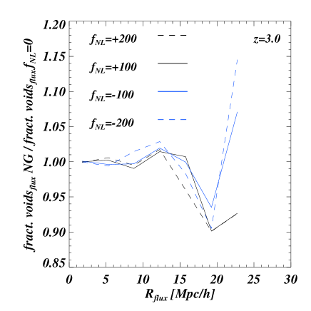
Figure 4: Ratio of the fraction of voids in the flux distribution between NG models and the corresponding Gaussian one at $z=3$ as a function of void size in comoving Mpc$/h$. The models with $f_{\rm NL}=-200,-100,+100,+200$ are represented by the blue dashed, blue continuous, black continuous and black dashed lines, respectively.

3.3 The Lyman-$\alpha$ flux power spectrum

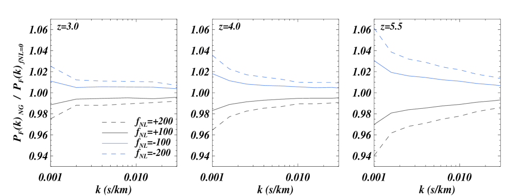
Figure 5: Ratio between the simulated 1D flux power spectrum of four different $(60,384)$ models with $f_{\rm NL}=-200,-100,+100,+200$ and $f_{\rm NL}=0$, represented by the blue dashed, blue continuous, black continuous and black dashed lines, respectively. Results are shown at at $z=3,4\ {\rm and}\ 5.5$ in the left, middle and right panels, respectively.

Primordial non-Gaussianity affects the evolution of density perturbation, particularly at the epochs and scales in which they enter the non-linear regime. Deviations from the Gaussian case are larger at high redshift, since at late times nonlinear dynamical effects become dominant. However, the contribution non-Gaussianity implied by $f_{\rm NL}=\pm 100$ is always within a few percent of the total gravitational potential and should not appreciably affect the linear matter power spectrum. Consequently, we also expect the effect on the 1D flux power spectrum to be small.

To quantify the effect we have plotted in Figure 5 the 1D flux power spectrum for the Gaussian and non-Gaussian cases at $z=3,4,\ {\rm and}\ 5.5$, in the left, middle and right panels respectively. Even in this case the QSO spectra have been normalized to reproduce the same mean flux. Differences to the Gaussian case are of the order of 2%, 3% and 5% at the redshifts considered here and manifest themselves as an overall plateau with slightly more power at the largest scales (a factor two larger than at the smallest scales probed). As expected, the effect of primordial non-Gaussianity on the flux power spectrum is small and the effect decreases with time.

In principle this effect on the flux power is degenerate only with a change in the mean flux level (see for example Figure 3 of Viel & Haehnelt (2006) or Figure 13 of McDonald et al. (2005)): this means that other changes in cosmological parameters and/or astrophysics produce a different $k$-dependent change in the flux power than the one produced by non-Gaussianities. However, the magnitude of this effect is quite small and probably not detectable with present data sets.

3.4 The Lyman-$\alpha$ flux bispectrum

Unlike the power spectrum, the bispectrum on large scales is sensitive to the statistical properties of primordial fluctuations like a primordial non-Gaussianity (Fry, 1994; Verde, 2002; Sefusatti & Komatsu, 2007). Therefore, the 1D flux bispectrum looks like a very promising statistics to search for non-Gaussianities in the IGM. The Lyman-$\alpha$ flux bispectrum has been calculated for the first time using high-resolution QSO spectra by Viel et al. (2004b). Here, we use the same definition i.e. the real part of the three point function in $k-$space $,D_{F}={\rm Re}(\delta_{F}(k_{1})\,\delta_{F}(k_{2})\,\delta_{F}(k_{3}))$, for closed triangles $k_{1}+k_{2}+k_{3}=0$. $\delta_{F}(k)$ is the Fourier transform of $\delta F$. $D_{F}$ is related to the bispectrum of the flux $B_{F}(k_{1},k_{2},k_{3})$

$$\langle D_{F}\rangle=2\,\pi\,B_{F}(k_{1},k_{2},k_{3})\,\delta^{D}(k_{1}+k_{2}+k_{3})\;.$$ (4)

$\delta^{D}(k)$ is the one-dimensional Dirac delta function and $\langle\cdot\rangle$ indicates the ensemble average. Since we compute the one-dimensional bispectrum our triangles are degenerate and we choose two configurations: $i)$ the flattened configurations for which $k_{1}=k_{2}$ and $k_{3}=-2\,k_{1}$; $ii)$ the squeezed configuration for which $k_{1}=k-k_{\rm min}$, $k_{2}=-k-k_{\rm min}$ and $k_{3}=2\,k_{\rm min}$, with $k_{\rm min}=2\pi/L$ (L the linear size of the box in km/s). In the following we will always show the flux bispectrum as a function of the wavenumber $k=k_{1}$. In Viel et al. (2004b) a numerical calculation of the flux bispectrum was compared to analytical estimates obtained through an expansion at second order of the fluctuating Gunn-Peterson approximation (Gunn & Peterson (1965)): while the overall amplitude of the bispectrum was not matched by the theory, the shape, at least at large scales, was well reproduced. However, the theoretical expression for the flux bispectrum contained only the gravitational terms. Here we extend this work by computing the flux bispectrum for NG Gaussian models using the numerical hydrodynamical simulations performed.

In Figure 6 we plot our findings in terms of ratios between the Gaussian and non-Gaussian models in the squeezed (top panels) and flattened (bottom panels) configurations. Due to the intrinsic noisy nature of the bispectrum, we have binned the values in $k-$space, in the same way as the flux power of the previous subsection.

One can see that while at $z=3$ the differences are very small and usually less than 3-4%, they become much larger and of the order of 30-40% at $z=4$. At $z=5.5$ the differences become again smaller and with different wavenumber dependence. It is possible to interpret this trend in the framework of the second order perturbation theory as done in Viel et al. (2004b): the overall amplitude and shape of the flux bispectrum could not be smooth and strongly depend (in a non-trivial way) on the redshift evolution of the coefficients that describe the evolution of the mean flux level and of the IGM temperature-density.

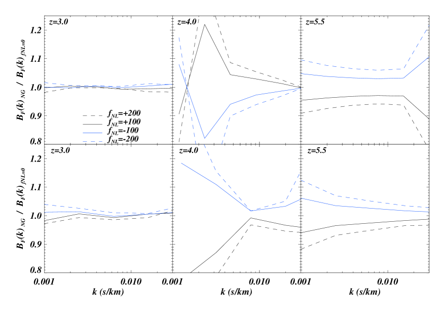
Figure 6: Ratio between the simulated 1D flux bispectrum in the flattened $(k,k,-2k)$ (bottom row) and squeezed configuration (top row) $(k-k_{min},-k-k_{min},2k_{min})$ with $k_{min}=2\pi/L$ (and with $L$ the linear size of the box in km/s) of four different $(60,384)$ models with $f_{\rm NL}=-200,-100,+100,+200$ and $f_{\rm NL}=0$, represented by the blue dashed, blue continuous, black continuous and black dashed lines, respectively. Results are shown at $z=3,4,5.5$ in the left, middle and right panel, respectively.

4 Discussion

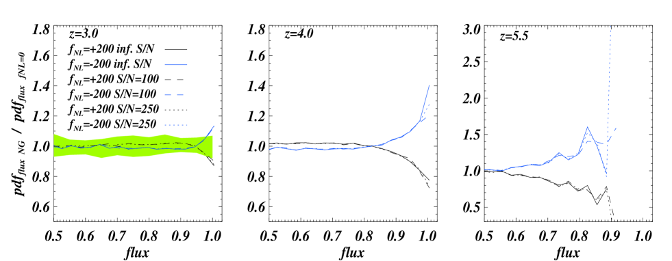
Figure 7: Ratio between the simulated flux probability distribution function of two different $(20,256)$ models with $f_{\rm NL}=-200,+200$ and the gaussian model with $f_{\rm NL}=0$, represented by the blue and black lines, respectively. The continuous lines are for an infinite signal-to-noise ratio, while dashed and dotted are for signal-to-noise ratios of 100 and 250. Results are shown at $z=3,4,5$ in the left, middle and right panels. The continuum errors are modelled as described in the text and are of the order 2% at $z=3$ and 10% at $z=4,5.5$. In the left panel we report as a filled area the statistical error bars of the flux PDF at $z=2.94$, as found in (Kim et al., 2007).

Among the different flux statistics that we have explored, the flux PDF seems the most promising in order to detect primordial non-Gaussiantity. However, to assess whether such information can actually be extracted from the real datasets one needs to compare the expected signal with the amplitude of the known errors. The present statistical uncertainties in the flux PDF at $z<3$ derived from high-resolution high signal-to-noise spectra is below 4-5%. This number was derived using jack-knife estimators from a suite of high-resolution high signal-to-noise ($>50$ and usually around 100) QSO spectra by Kim et al. (2007). This is smaller than the effect we are seeking and possibly the NG signature is degenerate with other effects such as a change in the temperature evolution of the IGM.

In Figure 7 we show in a quantitative way the effect of the observational errors on the flux PDF, at $z=3,4\ {\rm and}\ 5.5$. We use a realistic (observed) array of signal-to-noise values taken from Kim et al. (2007) at $z=2.94$. The signal-to-noise depends on the transmitted flux, and the average signal-to-noise value for the noise array taken turned out to be $\sim 100$.

The various curves in these plots are the same as in Fig. 3 for the $f_{\rm NL}=\pm 200$ cases only. The dashed refers to the realistic errors of Kim et al. (2007) corresponding to an average $S/N=100$. We also plot the case of a more favorable case with $S/N=250$ (dotted curve), while the infinite signal-to-noise error is represented by the continuous line. A second source of uncertainty is represented by continuum fitting errors that we have modelled in a statistical way that produces a $\pm 2\%$, $\pm 6\%$ and $\pm 10\%$ displacement of the continuum level at $z=3$ and at $z=4$ and $z=5.5$, respectively. These numbers have been derived by the estimates of Kim et al. (2007) and Becker et al. (2007) based on the analysis of high resolution and high signal-to-noise QSO spectra. To account for these errors we have adjusted the simulated continuum of the transmitted flux along every line-of-sight by factor $1\pm G$, where $G$ is a number drawn from Gaussian distributions with width 0.02, 0.06 and 0.1 at $z=3,4$ and $z=5.5$. This should provide a reasonable estimate of the continuum fitting errors effects on the flux PDF as long as these errors are Gaussian.

Of course, taking into account realistic signal-to-noise values and the continuum fitting errors reduces the significance of the NG signal. We find that for a signal-to-noise ratio of 100 (250) it is reduced by   40 % (20%) at $z=3$, in the same way at higher redshifts, where the NG signal is higher, we find similar values. The continuum fitting errors are somewhat more important and reduce the significance of the NG signal on the flux PDF for $f_{\rm NL}=\pm 200$ by $\sim 40\%$ at $z=3$. However, adding the two sources of errors at the same time as shown in Figure 7 decreases the NG signal by 45 %, 40% and 80% at $z=3,4,5.5$ for the $f_{\rm NL}=\pm 200$ cases, respectively.

The statistical errors estimated by Kim et al. (2007) are represented by the shaded area in the leftmost panel and refers to $z=2.94$. Ideally, one would like the NG signal to be larger than the statistical errors once all the systematic errors have been taken into account. At $z=3$ we are indeed in this case, but only marginally so. We find that the effect of including continuum uncertainties at $z=3$ has the same quantitative effect of dealing with a signal-to-noise ratio of 250 instead of an infinite one, and when these two errors are added together the effect on the flux PDF is of the same order of the NG signal for $f_{\rm NL}=\pm 200$. At higher redshifts the situation becomes slightly better. However, despite the reduction of the NG signal, its signature is still large enough to be detected, especially at $z>3$, and a higher significance could be of course reached once all the Lyman-$\alpha$ flux statistics (PDF, flux power and bispectrum) will be fitted at the same time.

We stress that our quantitative arguments do not include the possible degeneracies on the flux PDF of NG with other cosmological and astrophysical parameters as addressed in Bolton et al. (2008). It is however intriguing that a better fit to the PDF data presented there at $F>0.8$ would require emptier voids and thus negative values of $f_{\rm NL}$.

5 Conclusions and perspectives

In this work we have explored the possibility of constraining primordial non Gaussianity through the statistical properties of Lyman-$\alpha$ forest QSO spectra at $z\geq 3$. For this purpose, and for the first time, we have performed a suite of high resolution non-Gaussian hydrodynamical simulations. Although recent analyses have provided convincing evidence that the most stringent constraints to primordial non-Gaussianity will be likely provided by the large scale biasing properties of rare, massive objects (e.g. Slosar et al. (2008)), the analysis of the Lyman-$\alpha$ forest has to be regarded as complementary since it would probe non-Gaussianity on smaller scales and at intermediate epochs between other LSS probes and the CMB.

The main results of this study can be summarized as follows:

(i) the differences between the Gaussian and non-Gaussian scenarios are more evident in regions of high flux transmissivity associated to low density environments in the gas distribution;

(ii) deviations from the Gaussian case are best seen in the high flux tail of the 1D flux PDF: differences are of the order of 20-30 % and $z=3$ and increase up to $\sim 100$ % at $z=5.5$;

(iii) differences in the void distribution function are comparatively smaller, indicating that the PDF is a better statistics to spot primordial non-Gaussianity;

(iv) the 1D flux power spectrum is little affected by non-Gaussianity, as expected by the analogy with the matter power spectrum: the measured differences are of the order of a few per cent and increase at higher redshifts;

(v) the flux bispectrum represents a much more powerful statistics and potentially could provide strong constraints;

(vi) the significance of the non-Gaussian signal is highly reduced when one accounts for realistic signal-to-noise values in the measured flux PDF and continuum fitting errors at high redshifts; nevertheless, significant constraints on the non-Gaussianity can still be extracted from the analysis of the high flux tail of the flux PDF.

The statistical error bars on the flux power as measured using the SDSS data release 3 by McDonald (2006) are usually in the range 3-10 % (going from the small scales 0.01 s/km to the largest 0.001 s/km) in the range $z=2-4$, so the NG signal in this case is smaller than the statistical error (even though combining all the data points the error will be of the order on the power spectrum amplitude will become 0.6% and on its slope of $\pm$ 0.005). The SDSS data release 3 is based on a sample of 3035, increasing the number of observed QSO spectra will reduce further the statistical error by a factor $\sqrt{N_{QSO}}$ making the NG signature more evident, once the degeneracies with all the other cosmological and astrophysical parameters will be properly addressed.

Regarding the flux bispectrum, the present statistical error bars at $z\sim 2$ are of the order 50% Viel et al. (2004b), as derived from high-resolution spectra, a value that is much larger than what is expected from a non-Gaussian signal at that redshift, while this value is comparable to what could be seen at $z\sim 4$. Even in this case, in order to study in a precise way putative NG signatures in the flux bispectrum, more work is needed to address numerical convergence of the flux bispectrum and to incorporate the relevant physical processes that can affect its shape and amplitude down to smaller scales than those probed by the flux power.

The statistical error bars derived from present data sets of QSO spectra at high resolution in the flux PDF function are usually below 5% for high transmissivity regions. This value is basically determined by the signal-to-noise ratio of the spectra and, at least potentially, higher signal-to-noise ratios can be achieved and beat down this statistical error. This statistics seems promising due to the large number of QSO spectra available and to the better understanding of systematics. Among the possible systematics the most important is the uncertainty due to the continuum fitting errors which however could probably be significantly reduced at high redshifts with a better understanding and removal of the QSO continuum.

References

- Bartolo et al. (2004) Bartolo N., Komatsu E., Matarrese S., Riotto A., 2004, Phys. Rep., 402, 103
- Becker et al. (2007) Becker G. D., Rauch M., Sargent W. L. W., 2007, ApJ, 662, 72
- Bolton et al. (2005) Bolton J. S., Haehnelt M. G., Viel M., Springel V., 2005, MNRAS, 357, 1178
- Bolton et al. (2008) Bolton J. S., Viel M., Kim T.-S., Haehnelt M. G., Carswell R. F., 2008, MNRAS, 386, 1131
- Carbone et al. (2008) Carbone C., Verde L., Matarrese S., 2008, ArXiv e-prints, 806
- Carswell & Rees (1987) Carswell R. F., Rees M. J., 1987, MNRAS, 224, 13P
- Colberg (2008) Colberg J. M. e. a., 2008, MNRAS, 387, 933
- Crotts (1987) Crotts A. P. S., 1987, MNRAS, 228, 41P
- Dalal et al. (2008) Dalal N., Doré O., Huterer D., Shirokov A., 2008, Phys. Rev. D, 77, 123514
- Dobrzycki & Bechtold (1991) Dobrzycki A., Bechtold J., 1991, ApJ, 377, L69
- Duncan et al. (1989) Duncan R. C., Ostriker J. P., Bajtlik S., 1989, ApJ, 345, 39
- Faucher-Giguère et al. (2008) Faucher-Giguère C.-A., Lidz A., Hernquist L., Zaldarriaga M., 2008, ApJ, 688, 85
- Fry (1994) Fry J. N., 1994, Physical Review Letters, 73, 215
- Grinstein & Wise (1986) Grinstein B., Wise M. B., 1986, ApJ, 310, 19
- Grossi et al. (2008) Grossi M., Branchini E., Dolag K., Matarrese S., Moscardini L., 2008, MNRAS, 390, 438
- Grossi et al. (2007) Grossi M., Dolag K., Branchini E., Matarrese S., Moscardini L., 2007, MNRAS, 382, 1261
- Gunn & Peterson (1965) Gunn J. E., Peterson B. A., 1965, ApJ, 142, 1633
- Haardt & Madau (1996) Haardt F., Madau P., 1996, ApJ, 461, 20
- Hikage et al. (2008) Hikage C., Coles P., Grossi M., Moscardini L., Dolag K., Branchini E., Matarrese S., 2008, MNRAS, 385, 1613
- Hikage et al. (2006) Hikage C., Komatsu E., Matsubara T., 2006, ApJ, 653, 11
- Hui & Gnedin (1997) Hui L., Gnedin N. Y., 1997, MNRAS, 292, 27
- Kamionkowski et al. (2008) Kamionkowski M., Verde L., Jimenez R., 2008, ArXiv e-prints
- Kang et al. (2007) Kang X., Norberg P., Silk J., 2007, MNRAS, 376, 343
- Kim et al. (2007) Kim T. ., Bolton J. S., Viel M., Haehnelt M. G., Carswell R. F., 2007, MNRAS, 382, 1657
- Komatsu et al. (2008) Komatsu E., Dunkley J., Nolta M. R., Bennett C. L., Gold B., Hinshaw G., Jarosik N., Larson D., Limon M., Page L., Spergel D. N., Halpern M., Hill R. S., Kogut A., Meyer S. S., Tucker G. S., Weiland J. L., Wollack E., Wright E. L., 2008, ArXiv e-prints, 803
- Lesgourgues et al. (2007) Lesgourgues J., Viel M., Haehnelt M. G., Massey R., 2007, Journal of Cosmology and Astro-Particle Physics, 11, 8
- Lo Verde et al. (2008) Lo Verde M., Miller A., Shandera S., Verde L., 2008, Journal of Cosmology and Astro-Particle Physics, 4, 14
- Matarrese et al. (1986) Matarrese S., Lucchin F., Bonometto S. A., 1986, ApJ, 310, L21
- Matarrese & Verde (2008) Matarrese S., Verde L., 2008, ApJ, 677, L77
- Matarrese et al. (2000) Matarrese S., Verde L., Jimenez R., 2000, ApJ, 541, 10
- Mathis et al. (2004) Mathis H., Diego J. M., Silk J., 2004, MNRAS, 353, 681
- Matsubara (2003) Matsubara T., 2003, ApJ, 584, 1
- McDonald et al. (2005) McDonald P., Seljak U., Cen R., Shih D., Weinberg D. H., Burles S., Schneider D. P., Schlegel D. J., Bahcall N. A., Briggs J. W., Brinkmann J., Fukugita M., Ivezić Ž., Kent S., Vanden Berk D. E., 2005, ApJ, 635, 761
- McDonald (2006) McDonald P. e. a., 2006, ApJS, 163, 80
- Meiksin (2007) Meiksin A. A., 2007, ArXiv e-prints
- Messina et al. (1990) Messina A., Moscardini L., Lucchin F., Matarrese S., 1990, MNRAS, 245, 244
- Moscardini et al. (1991) Moscardini L., Matarrese S., Lucchin F., Messina A., 1991, MNRAS, 248, 424
- Ostriker et al. (1988) Ostriker J. P., Bajtlik S., Duncan R. C., 1988, ApJ, 327, L35
- Rauch et al. (1992) Rauch M., Carswell R. F., Chaffee F. H., Foltz C. B., Webb J. K., Weymann R. J., Bechtold J., Green R. F., 1992, ApJ, 390, 387
- Ricotti et al. (2000) Ricotti M., Gnedin N. Y., Shull J. M., 2000, ApJ, 534, 41
- Schaye (2001) Schaye J., 2001, ApJ, 559, 507
- Schaye et al. (2000) Schaye J., Theuns T., Rauch M., Efstathiou G., Sargent W. L. W., 2000, MNRAS, 318, 817
- Sefusatti & Komatsu (2007) Sefusatti E., Komatsu E., 2007, Phys. Rev. D, 76, 083004
- Seljak (2008) Seljak U., 2008, ArXiv e-prints, 807
- Slosar et al. (2008) Slosar A., Hirata C., Seljak U., Ho S., Padmanabhan N., 2008, Journal of Cosmology and Astro-Particle Physics, 8, 31
- Song & Lee (2008) Song H., Lee J., 2008, ArXiv e-prints
- Springel (2005) Springel V., 2005, MNRAS, 364, 1105
- Theuns et al. (1998) Theuns T., Leonard A., Efstathiou G., Pearce F. R., Thomas P. A., 1998, MNRAS, 301, 478
- Verde et al. (2001) Verde L., Jimenez R., Kamionkowski M., Matarrese S., 2001, MNRAS, 325, 412
- Verde (2002) Verde L. e. a., 2002, MNRAS, 335, 432
- Viel et al. (2008) Viel M., Colberg J. M., Kim T.-S., 2008, MNRAS, 386, 1285
- Viel & Haehnelt (2006) Viel M., Haehnelt M. G., 2006, MNRAS, 365, 231
- Viel et al. (2004) Viel M., Haehnelt M. G., Springel V., 2004, MNRAS, 354, 684
- Viel et al. (2004b) Viel M., Matarrese S., Heavens A., Haehnelt M. G., Kim T.-S., Springel V., Hernquist L., 2004b, MNRAS, 347, L26
- Viel et al. (2003) Viel M., Matarrese S., Theuns T., Munshi D., Wang Y., 2003, MNRAS, 340, L47
- Weinberg & Cole (1992) Weinberg D. H., Cole S., 1992, MNRAS, 259, 652