Abstract

One observes that a considerable level of confusion remains about some of those aspects of irreversibility, entropy generation and ‘the arrow of time’ which actually are well understood. This demands that great care must be taken in any discussion of irreversibility to use clear-cut notions and precise language in order to be definite about which property follows from which assumption. In this work, a novel toy model of ‘algebraic mechanics’ is presented that elucidates specific key aspects of entropy generation in a system with extremely simple reversible fundamental dynamics. It is argued why insights gained through a detailed quantitative study of this toy model also have to be taken into account for any realistic model of microscopic dynamics, classical or quantum alike. As irreversibility also touches upon the quantum mechanical measurement process (through the ‘proof’ of the ‘H-Theorem’), a simple way to address the tenacious question ‘when (and how) the wave function collapses’ is offered.

1 Introduction

One of the most fundamental observations is that most processes we experience daily are intrinsically irreversible (‘one cannot make grain from beer’). On the other hand, the fundamental laws governing the physics of the building blocks of our world – most importantly, gravity and quantum electrodynamics – feature time reversal symmetry. So, how can reversible microscopic behaviour give rise to irreversible collective macrophysical phenomena? When discussing this question, the situation is actually obscured by the interplay of a number of very different facets: for one, we know that the standard model of particle physics contains exotic CP-violating processes which (due to the CPT-theorem) must also violate time reversal symmetry, most notably the decay of neutral K-mesons. While these processes must have played an important role in the early Universe, in particular to establish the matter/antimatter asymmetry – if God would switch them off right at this instant by pressing a button, we would not expect this to have any consequence whatsoever anymore towards the observed asymmetry between ‘forward in time’ and ‘backward in time’. Another important aspect is that the expanding Universe has a dense, hot past, reaching back to the Big Bang, while it does not seem to have a corresponding fate in the future.

Important as it is to consider cosmological and field theoretic facets of the question of the nature of time asymmetry, this must not obscure that a number of crucial insights already can be obtained by studying properties of simple physical toy models: if some general observation can be shown to already follow from very simplistic assumptions, then the corresponding mechanisms also have to be taken into account when discussing irreversibility in the context of more realistic physical models. Furthermore, misconceptions about fundamental issues can easily give rise to serious misunderstandings in more involved situations.

2 Algebraic Mechanics

A toy model used to study aspects of irreversibility in systems with reversible microscopic physics should have a number of highly desirable characteristics:

• It should be governed by very simple fundamental processes that are manifestly time-reversal-symmetric.

• It should be possible to easily simulate the evolution of the system on a computer at no loss of accuracy due to discretisation errors or similar technological restrictions.

• It should be feasible to simulate a potentially large number of time steps with constant memory requirements.

• The number of states of the system should be large, but finite, and ideally, entropy computations should not involve any mathematics more advanced than high school level.

• The system must provide some model for the identification of macroscopic properties from microscopic configurations.

One system that nicely satisfies all these conditions is a lattice gas model of discernible particles in which the fundamental interaction is scattering between particles. This model furthermore is made exactly tractable numerically (i.e. free of accumulating rounding errors) by taking particle positions and velocities not to be real numbers, but elements of the finite field $\mathbb{F}_{p}$, with $p$ being a prime. For all the examples in the rest of this work, we will specifically choose $p=19$. While this trick simultaneously makes the number of microstates of the system finite, the resulting model then unfortunately only retains a formal resemblance to real world physics. Still, once the important insights have been established utilizing this model as a tool, one easily convinces oneself that many relevant properties can be lifted directly e.g. to a model of the dynamics of hard spheres. Major technical restrictions are that numerical computations then have to be done with ridiculously high precision, which also will depend on the length of the interval of time to be simulated. On the conceptual side, going to hard spheres will require replacing the simple counting of states (i.e. combinatorics) with more advanced measure theory.

These three rules provide an axiomatic specification of the behaviour of the ‘algebraic mechanics’ model:

• (Arithmetics) All arithmetics is to be done in the field $\mathbb{F}_{p}$, i.e. modulo the prime $p$. In the following, these arithmetic operations will be denoted by $+_{p},-_{p},\cdot_{p}$, etc.

• (World) The system consists of finitely many labeled (i.e. discernible) particles living on the cells of a two-dimensional $p\times p$ board. Their physical degrees of freedom hence consist of two position coordinates $(x,y)\in\mathbb{F}_{p}\times\mathbb{F}_{p}$ as well as two velocity coordinates $(v_{x},v_{y})\in\mathbb{F}_{p}\times\mathbb{F}_{p}$. Multiple particles may occupy the same site on the lattice.

• (Dynamics) Time advances in discrete steps. A single step consists of $p$ subsequent stages, where each stage consists of three subsequent phases: Motion, Scattering, Motion. In a ‘Motion’ phase, every particle’s coordinates are increased according to the particle’s velocities: $(x_{(n)}^{\prime},y_{(n)}^{\prime})=(x_{(n)}+_{p}v_{x,(n)},y_{(n)}+_{p}v_{y,(n)})$. In a ‘Scattering’ phase, particles’ positions are not updated, but whenever multiple particles occupy the same cell, their average velocity $\bar{v}$ is determined (using $\mathbb{F}_{p}$ arithmetics), and the velocity $v_{(n)}=\bar{v}+_{p}\Delta v_{(n)}$ of every particle in that cell is then replaced by $v_{(n)}^{\prime}=\bar{v}-_{p}\Delta v_{(n)}$. If $p$ or more particles occupy the same cell, no scattering happens in that cell (i.e. velocities are not changed).

One immediately notices that:

• A scattering phase does not change the average velocity of all particles occupying the same cell, hence ‘total momentum is conserved’.

• A stage is made up in such a way of phases that it (a) is inherently time-reversal-symmetric, and (b) involves changes to both positions and velocities.

• The rule to exclude scattering for cells containing $p$ or more particles manages to make the dynamics well-defined in every situation and retains interesting nontrivial scattering properties as long as the number of particles is not far larger than the number of cells.

• Systems which have been set up in such a way that scattering events do not take place – e.g. one particle per row, all of them moving horizontally only – return to their initial configuration after $p$ stages, i.e. one time step. Hence, under these rules, the time evolution of the system is governed by two- and multiparticle scattering processes.

The rules given here are simple enough to be easily implemented in Emacs Lisp, so that everybody’s favorite text editor can be used to study the behaviour of the system. A short piece of program code that implements a complete simulation framework is shown in appendix Appendix A:.

When starting from a very specific initial condition, such as a number of particles arranged as a compact block, with random initial velocities, one finds that for small block sizes, scattering processes are so rare that not much interesting happens on reasonable time scales. For our choice $p=19$, a $9\times 9$ block appears to be just of the right size to show interesting dynamics, as demonstrated in figure 1.

       T= 0                  T= 1                 T= 2
111111111..........  1111..1.1..........  1111.1111...1......
111111111..........  111.11111..........  111.11111........1.
111111111..........  111211111..........  11111111...........
111111111..........  1111.111...........  .111111............
111111111..........  11111111...........  111111111..........
111111111..........  11.111211..........  11.1.11.1..........
111111111..........  1...1.121..........  111.1..1...........
111111111..........  1.211.11...........  11111.11...........
111111111..........  .11111111..........  .1.111111..........
...................  ..............1....  ...................
...................  ....11.............  .....2.............
...................  .1.................  .1...........1....1
...................  ...................  .........1.........
...................  .1...............1.  ...................
...................  ...................  .................1.
...................  1...............1..  1..................
...................  ....1.......1......  ....1........1.....
...................  .............1.....  1............1....1
...................  ..................1  ............1.....1

        T= 5                 T=10                 T=20Ψ
1111.11.1.1........  1.1..1..1.1...1....  ..1..11.........1..
111.21111..........  121.111.1..1.......  ..11...21..1......1
11.111.11..........  1..1...1........1..  ......1.1...2...2..
.1.1.111...........  ..1...1........1.1.  ....2.2..........1.
.1111111...........  ..221111...........  ..1..11....1.......
11.111211..........  111.111.1..........  1....2..1..........
11....12...........  .1..11.............  .1.......11......1.
1.111.11...........  1.111.1.1.........1  1..1.........11....
.11111111..1.......  ..111.1....1....1..  ..11......1......1.
...................  1....1............1  ...........1.2....1
....11...........1.  ...1.1.............  ........1........1.
.1..........1......  .1........1.......1  .1..1.1...1....1...
.............1.....  ......1.1....1.....  11.....1..1..2...1.
.1.................  .1................1  1..................
..............11...  ........1.......11.  .1...............1.
1...............1..  .1...........11....  ...12...1....1.....
....1..............  .......1..21.1..1..  .1.....1..1.11.....
.............1....1  ....1..............  ...1...1....1..1...
.......1..........1  ............1......  1..............3...

Figure 1: Time evolution of a $9\times 9$ block of particles (example). Numbers denote the number of particles in a given cell, a dot denotes an empty cell.

In systems in which the ergodic hypothesis holds (or at least a weakened version thereof which claims that the system will trace out a substantial fraction of the accessible configuration space in an ‘effectively chaotic’ manner), asking the question what microstate the system is in at individual points in ‘macroscopic time’ (i.e. the scale of time differences is considerably larger than the time scale of microscopic processes) is equivalent to obtaining data from an uncorrelated source of randomness (such as a perfect die). Then, the Shannon entropy of such a random process just corresponds to the Boltzmann entropy of the physical system (up to a dimensionful proportionality constant required to match the statistical interpretation with the phenomenology of macroscopic thermodynamics).

Unfortunately, in a number of situations, the ergodic hypothesis is much more attractive than justifiable. In particular, we can consider ourselves lucky that the solar system does not seem to trace out all the mechanically possible configurations that would be allowed taking only the classical conservation laws into account. At first, this observation seems to be a major hurdle for the construction of a general theory explaining macroscopic phenomena in terms of microscopic processes. We will see, however, that the desirable link between Shannon and Boltzmann entropy can still be maintained even without invoking the ergodic hypothesis, if one is willing to pay a price in the form of a modified interpretation of macroscopic entropy.

2.1 The entropy of a source of randomness

If one had to define entropy in but a single sentence, then the statement that ‘Entropy is a linearly additive measure of the size of a space of possibilities’ presumably would be a strong contender: while being simple enough to be directly applied to a number of systems that can even be studied at school level – such as casting the die – it still contains all the relevant essence necessary to evolve the analytic formula for entropy both in coding theory and statistical mechanics, applying not much more than simple consistency considerations as well as quite elementary mathematics. In particular, Shannon’s entropy formula [1] is easily derived from consequent application of the three ideas that ‘rolling two perfect die produces twice as much randomness in every step as rolling just one dice’, ‘rolling five perfect die produces slightly less randomness than throwing thirteen perfect coins’, and ‘an imperfect dice that only rolls 1 and 2, with 50% probability each, is as a source of randomness equivalent to a perfect coin’. In particular, the entropy associated to some specific outcome is proportional to the logarithm of its rarity (inverse probability), and has to be weighted with the probability. Here, the logarithm ensures that entropy is additive when composing two independent systems, where the space of possible configurations grows multiplicatively. A useful choice of normalization is to associate an entropy of 1 to a perfect coin, denoting this amount of entropy a ‘bit’. This boils down to using the logarithmus dualis (base-2 logarithm) $\log{}_{2}={{\rm ld}\,{}}$ when defining entropy:

$$S=\sum_{i}p_{i}\,{{\rm ld}\,{1}}/p_{i}=\sum_{i}-p_{i}\,{{\rm ld}\,{p}}_{i}$$ (1)

One of the beauties of the ‘algebraic mechanics’ model is that we can easily compute the entropy as the logarithm of the number of microstate configurations that belong to a macrostate.

Considering a collection of $9\times 9=81$ labeled (i.e. discernible) particles moving on a $19\times 19$ lattice, the most generic macrostate description, which does not provide any additional constraints beyond this, can be realized through $\left(p^{4}\right)^{81}$ different microstates, as every particle can have arbitrary position and momentum, both being a pair of mod-p integers. The base-2 logarithm of this number gives the entropy of this macrostate, which is for $p=19$ just $4\cdot 81\cdot{{\rm ld}\,{1}}9\approx 1376.328514\,{\rm bit}$.

It is extremely important to note here that every constraint on the configuration of the particles can be translated to a set of microstates satisfying that constraint, so entropy is a property of a macroscopic description of a system, not the system itself! This means that different observers, which speak about the same system (i.e. microstate), but have a different degree of information about it, will associate different entropy to it. To make this point explicitly clear, let us consider the simple geometric pattern underlying the $T=0$ ‘initial’ configuration in figure 1. We will call this configuration $C_{0}$. Descriptions of $C_{0}$ of different level of detail correspond to different macrostates, hence different associated entropies:

• (MS1) A ‘blind’ observer who does not know anything about this configuration – except that “it contains 81 labeled particles” – will associate an entropy of $81\cdot 4\cdot{{\rm ld}\,{19}}\approx 1376.33\,{\rm bit}$ to it.

• (MS2) An observer who describes this configuration as “81 particles arranged in a regular $9\times 9$ pattern in the top left corner of the lattice, with unspecified velocities”, will associate to it an entropy of $81\cdot 2\cdot{{\rm ld}\,{19}}+{{\rm ld}\,{81!}}\approx 1089.33\,{\rm bit}$.

• (MS3) An observer describing the configuration as “all 81 particles being located somewhere in the top left $9\times 9$ corner of the lattice, with unspecified velocities” would associate to this description an entropy of $81\cdot 2\cdot{{\rm ld}\,{19}}+81\cdot 2\cdot{{\rm ld}\,{9}}\approx 1201.69\,{\rm bit}$.

• (MS4) An observer possessing detailed knowledge that “the first particle goes into the top-left corner, the second into column 2 in the first row, etc., but with unspecified velocities”, would associate to his description of the system the entropy $81\cdot 2\cdot{{\rm ld}\,{19}}\approx 688.16\,{\rm bit}$.

• (MS5) An observer having “detailed knowledge of the position and velocity (i.e. ‘as specified in the example program’) of each individual particle ” would associate to this description an entropy of $0\,{\rm bit}$.

• (MS6) An observer using data-reducing measuring devices that probe spatially averaged properties, such as in particular cumulative particle numbers in $3\times 3$ blocks (resp. $1\times 3$, $3\times 1$, $1\times 1$ blocks for the last row and column in the $19\times 19$ lattice), would see “nine particles in each of the $3\times 3$ top left blocks, and none in other positions”. Such a description would be associated to an entropy of $81\cdot 2\cdot{{\rm ld}\,{19}}+{{\rm ld}\,{\left(\left(9^{9}\right)^{9}\frac{81!}{9!^{9}}\right)}}\approx 1179.87\,{\rm bit}$.

It is especially this last case we will from now on be most concerned with.

2.2 Entropy generation over time

Starting from a configuration such as the one named config-a0 in the code example in the appendix, scattering processes will soon eradicate all visible structure. However, fundamental laws being explicitly time symmetric, we can always ‘respool’ the dynamics by just reversing all velocities. As there is a $1{:}1$ mapping between microstates at $T=0$ and microstates at any other time $T=T_{n}$ provided by time evolution, all that happens in this model is that easily visible spatial correlation is shifted to and mixed into more complicated correlations which are completely non-obvious to the human eye (not to speak of the fact that half the relevant information is missing in plots that do not show velocities). Experimenting with algebraic mechanics, one finds that – while we see perfect reversibility of time evolution – recurrence phenomena that reproduce initial configurations after an unexpectedly small number of time evolution steps (say, $\leq 1000$) nevertheless do not seem to occur (according to computer experiments).

When going from the time $T=T_{0}$ to any other time $T=T_{n}$, fully reversible microscopic dynamics guarantees that the macrostate (MS2) – as a set of $8.34\cdot 10^{327}$ microstates – evolves into another set of precisely the same number of microstates. Hence, entropy does not change with time in this process. This situation is completely analogous to the situation in classical mechanics, where Liouville’s theorem ensures the conservation of phase space volume. As there is a very terse textual description of the macrostate (MS2) at $T=0$, is there a similarly compact ‘articulated’ description of the macrostate which we get from (MS2) by time evolution? The best we can do is:

(MS2_(n)) A configuration which evolved out of a configuration that contained 81 particles in a regular $9\times 9$ pattern in the top left corner of the lattice, with unspecified velocities, by going from $T=0$ to $T=T_{n}$.

This linguistic trick demonstrates the actual conceptual idea underlying the mathematical proofs of entropy conservation in both classical as well as quantum systems whose dynamics is given by the Liouville-von Neumann equation. It should be noted that so far, our reasoning did not depend on whether $T_{n}$ lies in the future or in the past of $T_{0}$.

The kind of partial information which we have about any specific macroscopic system depends on the way our measuring devices work. From this perspective, we will almost exclusively encounter macrostates such as (MS6) when studying real systems: The way our measuring devices work strongly favors some macrostate descriptions over others. It is useful to introduce a special notion here: we want to call a macrostate whose description corresponds to information obtained(/in principle obtainable) about a set of microstates by applying some measuring apparatus $A$ an $A$-observed(/observable) macrostate. This idea allows us to define an entropy function $S_{A}$ that maps information obtained with the apparatus $A$ (say, a digital camera, or a thermometer, or both combined, a pair of human eyes, etc.) to the entropy of the macrostate description of all the microstates compatible with that observation.

Sticking with the example (MS6), the (specific) measuring apparatus $A$ that produces data of such form would embed the $19\times 19$ lattice into a $21\times 21$ lattice by adding two extra rows and columns to the right and bottom for bookkeeping purposes only – i.e. particles are forbidden to go there – and measure the number of particles in each of the $7\times 7$ blocks of size $3\times 3$ in the enlarged lattice. All information about particle identity as well as velocity is omitted, only locally averaged information about spatial distribution is determined. Explicitly, the number of microstates corresponding to a measurement that gave $N_{j}$ particles in the $3\times 3$ block $b_{j}$ is:

$$N=19^{2\cdot 81}\left(\prod_{j=1}^{7\times 7}|b_{j}|^{N_{j}}\right)\cdot\frac{81!}{\prod_{k=1}^{7\times 7}N_{k}!}$$ (2)

where $|b_{j}|$ is the number of real cells in the block $b_{j}$, normally 9, but for blocks that contain ‘padding cells’ this may be $3$ or $1$.

Time evolution from $T_{0}$ to $T_{n}$ maps the configuration (microstate) $C_{0}$ to some specific other configuration $C_{n}$. The evolution of entropy $S_{A}(C_{n})$ as measured by the apparatus $A$ with time is displayed in figure 2, both for evolution towards the future as well as evolution towards the past.

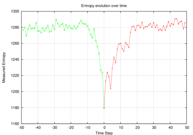
Figure 2: Time evolution of the $A$-observed macrostate entropy.

Here, it must be pointed out that, while $C_{0}$ is a very special configuration amongst all those microstates that belong to the macrostate (MS6), the behaviour observed is essentially the same for a generic microstate that belongs to (MS6): entropy increases both towards the past as well as the future, and also fluctuates. This claim is easily checked by using the function random-microstate-compatible-with-macrostate from the code given in the appendix. This produces a random, hence (usually) generic, microstate corresponding to a given $A$-observed macrostate.

2.3 Interpretation

The three crucial ingredients that produce the behaviour shown in figure 2 are:

• A collection of macrostates that are linked to the behaviour of a ‘data-reducing’ measuring device, which reports some kind of reduced information about the microstate configuration the system is in.

• Microscopic dynamics that is not aligned (i.e. does not respect) the data reduction associated with the measuring device.

• An initial state which, from the perspective of the measuring device, belongs to a macrostate which is special in the sense that its observed properties constrain the number of associated microstates relative to the number of microstates associated to a generic (again with respect to the measuring device) macrostate.

In real systems where the number of degrees of freedom usually is ridiculously large, the first condition is satisfied automatically by any conceivable measuring device. Usually, both omission and averaging over degrees of freedom are involved here. The second condition also is rather generic.

So, whenever reversible microscopic dynamics does not care about the macroscopic notions we use to describe the processes it causes at macroscopic, ‘averaged’ scales (which practically always is the case), we expect to encounter the situation that time evolution does not change the entropy of the macrostate, but finding a new description of the evolved macrostate in terms that are discernible by the measuring device does. It is this process of ‘re-articulation’ in which information about the macrostate is lost, and hence entropy increases. The information lost is precisely that part of the original knowledge about the system (in this example: averaged positional information) which – by the dynamics – was mixed into more complicated correlations not detected by the measuring apparatus.

Simply stated, entropy increases whenever we apply dynamics to partial knowledge about a system and eventually project back onto the same class of partial system descriptions used initially, unless these descriptions are compatible with the microscopic dynamics. As there is no intrinsic reason why they should be, this is normally the case – but with this criterion in mind, it also is easy to construct counter-examples (a trivial one being translational motion of a single solid body). In particular, entropy also increases when we go from the ‘present’ to the ‘past’: Just as it is difficult to draw conclusions about the future by studying the present, it is also difficult to draw conclusions about the past. Generally speaking, if the situation were so simple that the idea that ‘entropy increases with time’ described everything there is to know, we should not have much difficulty answering a question such as ‘where does the moon come from’? While a description of a system’s past may well correspond to a low entropy macrostate, we can still easily encounter the situation that, for a given system, the totality of all conceivable pasts (each of which may well have low entropy) that are compatible with our knowledge is a macrostate of higher entropy than the one describing the present situation.

In this toy system, the magnitude of entropy increase is just a measure of the amount of information lost by going from a description such as ‘evolved out of a system characterized by macroscopic parameters $P_{0}$ at time $T_{0}$’ to a description ‘characterized by macroscopic parameters $P_{n}$ at time $T_{n}$’. Evidently, the latter macrostate cannot contain fewer microstates than the former: perfect traceability would mean that we can identify the image of each microstate under the one-to-one mapping of time evolution. Less-than-perfect traceability means that the number of possibilities increases. This is analogous to the very basic observation that, when adding the numbers 3 and 5, and keeping the result while forgetting the summands, the number 8 ‘does not know how it was produced’ – it may also have been the result of adding 6 to 2. So, in this ‘irreversible addition’, we ‘produced entropy’.

The observed ‘fluctuations’ on top of the gradual increase in entropy (which may lead to transient decreases in entropy) correspond to those situations where the association of macrostates to subsequent microstates happened to produce a ‘comparatively small’ macrostate following a larger one. When investigating the dynamics of a single microstate only, such processes are a priori not excluded, and certainly expected to determine the behaviour of the system at times far away from $T_{0}$. If we started instead from an uniformly weighted collection of all microstates that represent a given macrostate $M$, then re-articulation after time evolution would produce a weighted collection of new $A$-observed macrostates. As a weighted collection of macrostates again is a macrostate (but usually not an $A$-observable one), and as this re-articulated description contains extra microstates in addition to the time-evolution images of the microstates in $M$, the entropy of this less stringent description is larger than the entropy of $M$: the re-articulation projection loses information about the time-evolved system. In this sense, the increase in entropy is inevitable. If we started from any macrostate that is projected onto a specific $A$-observable macrostate, but contains less microstates (e.g. only a single one), then there is hidden information about the system: its state could be known more accurately than how it is described by the corresponding $A$-observable macrostate. The dynamics will mix this hidden information to a varying degree with those parameters the measuring device $A$ is sensitive to, hence giving rise to entropy fluctuations. Considerations on ‘Maxwell’s Daemon’ show that the magnitude of these fluctuations gives a lower bound on the minimal effort any physical realization of the measuring device $A$ must make.

2.4 Additional remarks

Putting insights gained by studying the ‘algebraic mechanics’ toy model into proper physical context requires a few additional remarks.

2.4.1 Quantum Mechanics, the measurement process, and the ‘H-Theorem’

Computing the rate of change of entropy by applying the Liouville-von Neumann equation to the quantum mechanical expression for entropy ($S=-k_{B}{{\rm tr}\,{\rho\,\ln\rho}}$) gives the result that entropy is conserved. This situation is analogous to the situation encountered in the toy model when omitting the step of ‘re-articulation’. One easily convinces oneself (e.g. by means of an example) that the quantum mechanical density matrix reduction associated with the measurement process changes (increases) entropy. This again is associated to an information-lossy projection, usually called a ‘quantum jump’. Just as with the question about entropy generation, there is substantial confusion about the question ‘when (and how) the wave function collapses’ (e.g. whether this is a ‘faster-than-light’ process). As ‘quantum jumps’ lead to an increase of entropy, some relevant aspects are actually linked, and so are explanations. Considering a combined system consisting of a ‘quantum device’ Q (e.g. an excited atom) and a ‘measuring device’ D (e.g. a detector), the quantum states of the combined system are elements of the tensor product Hilbert space $\mathcal{H}_{Q}\otimes\mathcal{H}_{D}$. Due to the interaction between Q and D, the ‘initial time’ quantum states of the form $|q,d\rangle_{-}$ evolve into entangled linear combinations. In other words, the final quantum states $|q,d\rangle_{+}$ we would like to use to describe the system with after the interaction give us a different basis (in the Heisenberg picture) than that of the initial quantum states. As one all too often thinks of these quantum states in terms of position space probability amplitudes, where they look the same, it is deceptively easy to get confused by failing to discern between elements of the ‘initial’ Hilbert space $\mathcal{H}_{-}$ and the ‘final’ Hilbert space $\mathcal{H}_{+}$ (which are isomorphic). Evidently, every description of a measurement process will at some point have to make the transition from using quantum states in $\mathcal{H}_{-}$ to using quantum states in $\mathcal{H}_{+}$. It is precisely at this point in the description of the process where this transition happens that ‘the wave function collapses’, if it is done in such a way that phase correlation information is lost through projection. Regardless of whether this step is consciously articulated or not, it will have to happen somewhere in every description of a measurement process. Consequently, the confusion of conceptual levels associated with the question ‘whether the collapse of the wave function is a faster-than-light process’ is of the same kind as the confusion demonstrated by the question-answer combination ‘why the maid in Shakespeare’s poem A Lover’s Complaint is pale’ / ‘because it rhymes with tale’: Here, the question was posed at the level of content, while the answer was given at the level of description.

This has to be taken into account when using quantum jumps and Fermi’s Golden Rule to justify a Markov model as a basis for a proof of the quantum mechanical version of Boltzmann’s ‘H-Theorem’ [3]. (Essentially, this then amounts to proving entropy generation by assuming entropy generating irreversible fundamental processes.)

2.4.2 Physical relevance of the toy model

The key property of the ‘algebraic mechanics’ model is its perfect computational traceability without losses related to numerical limitations. While this helps to simplify a number of arguments, the relevant reasoning can be lifted naturally to more realistic descriptions of microscopic physics that cannot avoid the problem of limited numerical precision. This basically means to wrap up most statements in constructions such as ‘If one demands numerical precision X on initial states, then for the given amount of time to pass, the following holds within numerical precision Y: …’ where the precision-related errors can be made small. Apart from complicating the discussion, this does not introduce qualitatively new features. Therefore, the value of the toy model lies in helping to isolate relevant aspects that lead to important insights from irrelevant ones.

Additionally, while this is not the subject of this work, there are situations where information about the behaviour of a ‘continuous’ system can be gained by studying its behaviour in modulo-$p$ arithmetics. Presumably the most famous example of such a situation is given by the Grothendieck-Katz conjecture [4].

3 Conclusion

The ‘algebraic mechanics’ toy model introduced here is both simple and powerful enough to elucidate some key aspects of the phenomenon of the thermodynamic arrow of time in terms accessible to a broad audience. Other toy models that demonstrate entropy generation based on reversible microscopic dynamics exist, such as the Kac ring model [5] (also see [6]). The conceptual advantage of the very simple ‘algebraic mechanics’ toy model is that model unifies exact computational traceability with formal similarity to mechanics. It demonstrates entropy generation with respect to time evolution towards the future as well as towards the past, and gives interpretations of this phenomenon through the notion of ‘re-articulation’.

Any ‘measurement’ involves data reduction. In fact, considering the situation in quantum computing, it may be appropriate to define ‘a measurement’ as ‘a data-reducing projection’. If the microscopic dynamics does not respect (i.e. is agnostic about) the eigenspaces of this projection, then time evolution followed by re-articulation will lead to an inevitable loss of information contained in the system’s description. Hence, as soon as we use dynamics to extract useful information about a system at any other time than the present, we see an increase in entropy, regardless of whether time evolution was performed towards the future or towards the past. When asking questions about the future, we will hence observe entropy to increase towards the future. When doing forensic analysis, we observe the opposite phenomenon: Extracting information about how precisely an accident happened gets increasingly difficult the more time has passed since.

When discussing entropy generation (and also the quantum mechanical measurement process), great care has to be taken to discern between concepts that refer to two different levels: the ‘fundamental dynamics level’ and the ‘description level’. While conclusions that can be obtained by studying this toy model leave open many important questions about the physical ‘arrow of time’ (e.g. why the universe has a hot past), it is important to first understand what aspects of entropy generation already follow from very basic general features – before more advanced physics can be discussed.

Strictly speaking, this work says nothing new about physical processes (e.g. fundamental dynamics). Furthermore, it does not offer new descriptions of physical processes (i.e. thermodynamics). It does, however, address some occasionally discussed issues concerning the descriptions of descriptions of physical processes.

Philosophical aspects

One important source of confusion in the discussion of the ‘arrow of time’ is the philosophical question of determinism: is the future determined by the past? Stated differently, if all information about the world were contained in a spatial slice, and ‘dynamics’ were nothing else but some invented funny mathematics on top of such an initial configuration that meaninglessly maps it to other configurations, why should e.g. some form of ‘dynamical laws’ be more ‘real’ than another possible imagined choice? Physically speaking, asking ‘whether the world is deterministic or not’ a priori is as much a non-question as is the question ‘why anything exists at all’: As it is impossible to perform experiments on ‘the whole world’, the toolbox of physics cannot give an answer – the only way to come up with an answer is to first find out how the question one had in mind should have been phrased accurately. Evidently, we can ask whether some specific process in a system we can isolate and experiment with is ‘deterministic’. If a key property of all experiments is the separation of the system measurements are performed on from ‘something else’, then the question whether ‘the world is deterministic’ is nonphysical in precisely the same way as the question ‘what happens if an unstoppable force meets an unmoveable object’, due to a fundamental contradiction in the assumptions. Certainly, as abolishing relevant prejudice is an important prerequisite for gaining insight by means of the scientific method, discussing the ‘arrow of time’ mandates overcoming all prejudice on determinism first. While this work demonstrates that the phenomenon of ‘observed entropy generation’ already happens in an extremely simple completely deterministic toy model, and reasons that the underlying mechanisms are basic enough to generalize to virtually all more realistical physical models, this does not at all touch the question whether some particular fundamental physics actually follows deterministic laws or not.

Acknowledgments

The original incentive for this work came from a request to explain in more detail the physical aspects of a popular talk on the ‘thermodynamic arrow of time’ given by the author at the interdisciplinary MinD Congress on ‘Time’ in Nuremberg (Nürnberg), Germany, 02.10. – 05.10.2008. The ‘algebraic mechanics’ model was developed subsequently in an effort to construct a maximally simple easily traceable quantitative explanation of a key phenomenon underlying entropy generation. It hence is a pleasure to thank Martin Dresler for asking the right question – namely for asking for a simple quantitative explanation of entropy generation also accessible to non-physicists.

Appendix Appendix A: Appendix: Emacs Lisp Code

This piece of code, when loaded into the (X)Emacs editor with:
(byte-compile-and-load-file "amech.el")
allows the simulation of the ‘algebraic mechanics’ toy system:

(require ’cl)

(defun v-init (n f)
  (let ((v (make-vector n nil)))
    (dotimes (j n) (setf (aref v j) (funcall f j)))
    v))

(defmacro xlambda (args &rest body)
  ‘(lambda ,args
     (lexical-let ,(mapcar (lambda (n) (list n n)) args) . ,body)))

(defconst amech-prime 19)

(setf amech-div-table
  (v-init amech-prime
          (xlambda (n)
                   (let ((vn (v-init amech-prime
                                     (xlambda (x) (mod (* x n) amech-prime)))))
                     (position 1 vn)))))

(defun a+ (x y) (mod (+ x y) amech-prime))
(defun a- (x y) (mod (- x y) amech-prime))
(defun a* (x y) (mod (* x y) amech-prime))
(defun a/ (x y) (mod (* x (aref amech-div-table y)) amech-prime))
(defun va+ (vx vy) (cons (a+ (car vx) (car vy)) (a+ (cdr vx) (cdr vy))))
(defun va- (vx vy) (cons (a- (car vx) (car vy)) (a- (cdr vx) (cdr vy))))
(defun va/ (vx n)  (cons (a/ (car vx) n) (a/ (cdr vx) n)))

(defun advance-time (config &optional nr-steps)
  (dotimes (step (or nr-steps 1) config)
    (let* ((v00 ’(0 . 0))
           (advance (lambda (p) (cons (va+ (car p) (cdr p)) (cdr p))))
           (new-config-1
            (let* ((c (mapcar advance config))
                   (ht-by-pos (make-hash-table :test ’equal)))
              (dolist (np c)
                (push np (gethash (car np) ht-by-pos nil)))
              (maphash
               (lambda (pos particles)
                 (when (< (length particles) amech-prime)
                   (let* ((v-avg (va/ (reduce #’va+ particles
                                              :initial-value v00 :key #’cdr)
                                      (length particles)
                                      )))
                     (dolist (p particles)
                       (setf (cdr p) (va- v-avg (va- (cdr p) v-avg)))))))
               ht-by-pos)
              c))
           (new-config-2 (mapcar advance new-config-1)))
      (setf config new-config-2))))

(defun reverse-velocities (config)
  (mapcar (lambda (p) (cons (car p) (va- ’(0 . 0) (cdr p)))) config))

(defun display-config (config)
  (macrolet ((ic (spec)
                 ‘(let (($x ,spec))
                    (setf ,spec (if (eql $x ?.) ?1
                                  (int-char (+ 1 (char-int $x))))))))
    (let ((board (v-init amech-prime
                         (lambda (n) (make-string amech-prime ?.)))))
      (dolist (particle config)
        (ic (aref (aref board (cdar particle)) (caar particle))))
      (dotimes (j amech-prime)
        (insert (format "\n%s" (aref board j))))))
  (insert "\n") t)

(defun log2-fakt (n)
  (if (= n 0) 0.0
    (+ (/ (log n) (log 2.0)) (log2-fakt (- n 1)))))

(defun config-entropy (config)
  ;; "Measuring" entropy with the device model described in the main text
  (let* ((nr-blocks (ceiling (/ amech-prime 3.0)))
         (boundary (mod amech-prime 3)) ; never =0!
         (b-sizes
          (let ((v (make-vector (* nr-blocks nr-blocks) 9)))
            (dotimes (j nr-blocks)
              (setf (aref v (+ (* nr-blocks j) nr-blocks -1))
                    (* boundary
                       (/ (aref v (+ (* nr-blocks j) nr-blocks -1)) 3))))
            v))
         (counts (make-vector 49 0)))
    (dolist (p config)
      (let* ((xpos (floor (caar p) 3))
             (ypos (floor (cdar p) 3))
             (nr-cell (+ (* ypos 7) xpos)))
        (incf (aref counts nr-cell))))
    (labels
        ((entropy (nr-cell sum)
           (if (= nr-cell 49)
               (reduce (lambda (sf x) (- sf (log2-fakt x)))
                       counts :initial-value (+ sum (log2-fakt 81)))
             (entropy (+ 1 nr-cell)
                      (+ sum (* (aref counts nr-cell)
                                (/ (log (aref b-sizes nr-cell))
                                   (log 2.0))))))))
      (+ (entropy 0 0.0)
         (* 81 2 (/ (log 19) (log 2)))))))

(defun random-microstate-compatible-with-macrostate (n-per-3x3)
  (let ((config nil) (size (length n-per-3x3)))
    (dotimes (j size)
      (dotimes (k size)
        (let ((n (aref (aref n-per-3x3 j) k)))
          (dotimes (m n)
            (push
             ‘((,(+ (* 3 j) (random (min 3 (- amech-prime (* 3 j))))) .
                ,(+ (* 3 k) (random (min 3 (- amech-prime (* 3 k))))))
               . (,(random amech-prime) . ,(random amech-prime)))
             config)))))
    config))

(defconst config-a0
  (if nil
      ;; roll the die to produce a random configuration:
      (let ((k 9))
        (coerce (v-init (* k k)
                        (lambda (n) ‘((,(floor (/ n k)) .
                                       ,(mod n k)) . (,(random amech-prime) .
                                                      ,(random amech-prime)))))
                ’list))
    ;; Use a definite initial configuration:
    ’(((0 . 0) 14 . 15) ((0 . 1) 0 . 10) ((0 . 2) 6 . 8) ((0 . 3) 0 . 7)
      ((0 . 4) 10 . 18) ((0 . 5) 16 . 4) ((0 . 6) 13 . 7) ((0 . 7) 12 . 13)
      ((0 . 8) 17 . 1) ((1 . 0) 8 . 9) ((1 . 1) 9 . 8) ((1 . 2) 4 . 17)
      ((1 . 3) 1 . 5) ((1 . 4) 14 . 9) ((1 . 5) 16 . 15)  ((1 . 6) 9 . 12)
      ((1 . 7) 11 . 10) ((1 . 8) 3 . 17) ((2 . 0) 18 . 3) ((2 . 1) 6 . 10)
      ((2 . 2) 2 . 4) ((2 . 3) 15 . 16) ((2 . 4) 11 . 8) ((2 . 5) 10 . 10)
      ((2 . 6) 10 . 18) ((2 . 7) 1 . 0) ((2 . 8) 8 . 6) ((3 . 0) 18 . 9)
      ((3 . 1) 11 . 13) ((3 . 2) 18 . 9) ((3 . 3) 10 . 9) ((3 . 4) 2 . 2)
      ((3 . 5) 0 . 5) ((3 . 6) 0 . 0) ((3 . 7) 9 . 7) ((3 . 8) 10 . 11)
      ((4 . 0) 11 . 6) ((4 . 1) 9 . 4) ((4 . 2) 15 . 1) ((4 . 3) 14 . 6)
      ((4 . 4) 0 . 15) ((4 . 5) 6 . 9) ((4 . 6) 2 . 6) ((4 . 7) 18 . 14)
      ((4 . 8) 0 . 18) ((5 . 0) 4 . 10) ((5 . 1) 9 . 6) ((5 . 2) 13 . 10)
      ((5 . 3) 11 . 14) ((5 . 4) 10 . 1) ((5 . 5) 2 . 2) ((5 . 6) 13 . 14)
      ((5 . 7) 8 . 4) ((5 . 8) 18 . 5) ((6 . 0) 5 . 13) ((6 . 1) 11 . 5)
      ((6 . 2) 10 . 17) ((6 . 3) 15 . 13) ((6 . 4) 5 . 15) ((6 . 5) 8 . 6)
      ((6 . 6) 14 . 12) ((6 . 7) 17 . 5) ((6 . 8) 0 . 11) ((7 . 0) 15 . 12)
      ((7 . 1) 6 . 7) ((7 . 2) 14 . 9) ((7 . 3) 9 . 8) ((7 . 4) 4 . 18)
      ((7 . 5) 12 . 4) ((7 . 6) 4 . 17) ((7 . 7) 17 . 15) ((7 . 8) 4 . 9)
      ((8 . 0) 14 . 0) ((8 . 1) 3 . 0) ((8 . 2) 16 . 11) ((8 . 3) 7 . 11)
      ((8 . 4) 5 . 5) ((8 . 5) 17 . 6) ((8 . 6) 16 . 13) ((8 . 7) 18 . 4)
      ((8 . 8) 2 . 13))))

(defconst config-a1
   ;; use this to check the claim of the genericity of entropy evolution
   ;; over time
  (if nil
    (random-microstate-compatible-with-macrostate
     [[9 9 9 0 0 0 0] [9 9 9 0 0 0 0] [9 9 9 0 0 0 0]
      [0 0 0 0 0 0 0] [0 0 0 0 0 0 0] [0 0 0 0 0 0 0]
      [0 0 0 0 0 0 0]])
  ’(((8 . 6) 11 . 1) ((6 . 6) 8 . 12) ((6 . 6) 17 . 0) ((6 . 6) 11 . 3)
    ((8 . 8) 3 . 5) ((8 . 6) 16 . 11) ((8 . 8) 9 . 5) ((6 . 6) 16 . 6)
    ((7 . 8) 12 . 18) ((8 . 5) 3 . 8) ((6 . 5) 11 . 14) ((7 . 3) 0 . 6)
    ((8 . 4) 1 . 10) ((7 . 3) 12 . 11) ((6 . 4) 16 . 2) ((7 . 4) 12 . 17)
    ((7 . 4) 11 . 3) ((8 . 5) 6 . 7) ((8 . 2) 17 . 4) ((8 . 2) 3 . 8)
    ((6 . 1) 18 . 8) ((8 . 2) 6 . 10) ((7 . 2) 18 . 18) ((7 . 2) 14 . 8)
    ((7 . 1) 4 . 4) ((7 . 2) 1 . 1) ((7 . 2) 11 . 8) ((3 . 7) 0 . 13)
    ((4 . 7) 2 . 7) ((4 . 6) 15 . 7) ((5 . 7) 2 . 9) ((4 . 6) 13 . 9)
    ((4 . 7) 10 . 2) ((5 . 7) 7 . 11) ((4 . 6) 15 . 16) ((5 . 8) 4 . 11)
    ((5 . 4) 12 . 14) ((4 . 5) 17 . 6) ((5 . 5) 15 . 11) ((4 . 5) 9 . 10)
    ((5 . 5) 4 . 17) ((4 . 5) 16 . 10) ((5 . 5) 17 . 3) ((5 . 3) 2 . 9)
    ((5 . 5) 12 . 5) ((4 . 2) 3 . 6) ((3 . 0) 5 . 4) ((3 . 1) 13 . 10)
    ((3 . 0) 1 . 13) ((4 . 2) 15 . 12) ((4 . 1) 9 . 7) ((4 . 0) 10 . 16)
    ((5 . 2) 13 . 5) ((3 . 1) 10 . 17) ((1 . 7) 5 . 14) ((1 . 6) 10 . 0)
    ((0 . 7) 4 . 7) ((2 . 8) 3 . 7) ((0 . 7) 2 . 12) ((1 . 8) 5 . 4)
    ((1 . 6) 4 . 14) ((1 . 8) 6 . 15) ((1 . 6) 15 . 5) ((0 . 3) 17 . 3)
    ((1 . 4) 4 . 15) ((1 . 3) 11 . 9) ((1 . 4) 5 . 16) ((0 . 4) 10 . 10)
    ((1 . 5) 13 . 8) ((2 . 3) 0 . 1) ((0 . 4) 5 . 12) ((0 . 4) 16 . 1)
    ((0 . 1) 18 . 13) ((0 . 0) 16 . 13) ((1 . 0) 14 . 14) ((2 . 1) 17 . 2)
    ((0 . 0) 13 . 12) ((1 . 1) 15 . 7) ((2 . 1) 9 . 3) ((1 . 2) 9 . 2)
    ((1 . 2) 11 . 5))))


(defun show-evolution (config &optional n tag offset)
  (dotimes (j (or n 10) t)
    (insert (format "\n====== %3s %3d %8.3f ======"
                    (or tag "T") j (config-entropy config)))
    (display-config config)
    (setf config (advance-time config amech-prime)))
  config)

(defun amech-demo (&optional config n)
  (let ((start-config (or config config-a0))
        (nsteps (or n 50))
        (config-at nil) (config-rat nil) (config-a00 nil))
    (setf config-at (show-evolution start-config nsteps "T+"))
    (setf config-rat (reverse-velocities config-at))
    (insert (format "\n[*****************]"))
    (display-config config-rat)
    (insert (format "[*****************]\n"))
    (setf config-a00 (show-evolution config-rat (+ 1 nsteps) "T-" 1))
    (equal config-a00 start-config)))

(amech-demo)

References

- [1] C. Shannon, ‘A mathematical theory of communication’, reprinted in: ACM SIGMOBILE Mobile Computing and Communications Review, Volume 5, Issue 1 (January 2001), 3-55.
- [2] S. Meretzky, ‘Leather Goddesses of Phobos’, Infocom, 1986 (Commodore 64). Cf. http://infocom.elsewhere.org/gallery/leather/leather.html
- [3] L. Boltzmann, ‘Weitere Studien über das Wärmegleichgewicht unter Gasmolekülen’, Wien. Ber. 66 (1872), 275-380.
- [4] N. Katz, ‘A conjecture in the arithmetic theory of differential equations’, Bull. Soc. Math. de France, 110 (1982), 203-239.
- [5] M. Kac, ‘Probability and Related Topics in the Physical Sciences’, Interscience Pub., New York, 1959.
- [6] J. Bricmont, ‘Science of Chaos or Chaos in Science?’, Annals of the New York Academy of Sciences, 1996 - Blackwell Synergy, arXiv: chao-dyn/9603009