Quantum entanglement in a non-commutative system

S. Adhikari satyabrata@bose.res.in S. N. Bose National Centre for Basic Sciences, Salt Lake, Kolkata 700 098, India    B. Chakraborty biswajit@bose.res.in S. N. Bose National Centre for Basic Sciences, Salt Lake, Kolkata 700 098, India    A. S. Majumdar archan@bose.res.in S. N. Bose National Centre for Basic Sciences, Salt Lake, Kolkata 700 098, India    S. Vaidya vaidya@cts.iisc.ernet.in Centre For High Energy Physics, Indian Institute of Science, Bangalore 560012, India
Abstract

We explore the effect of two-dimensional position-space non-commutativity on the bipartite entanglement of continuous variable systems. We first extend the standard symplectic framework for studying entanglement of Gaussian states of commutative systems to the case of non-commutative systems residing in two dimensions. Using the positive partial transpose criterion for separability of bipartite states we derive a new condition on the separability of a non-commutative system that is dependent on the noncommutative parameter θ𝜃\theta. We then consider the specific example of a bipartite Gaussian state and show the quantitative reduction of entanglement originating from non-commutative dynamics. We show that such a reduction of entanglement for a non-commutative system arising from the modification of the variances of the phase space variables (uncertainty relations) is clearly manifested between two particles that are separated by small distances.

pacs:
11.10.Nx,03.65.Ud

I Introduction

It is a common expectation that spacetime may not retain its smooth continuous structure at very short distances, and hence can have important consequences for physics at very high energies, like quantum gravity. Moyal deformation of ordinary spacetime is an example of a specific algebraic realization of this expectation dfr . Clarification of the role of underlying spacetime symmetries Chaichian:2004za ; aschieri is crucial for formulating quantum dynamics on such spaces bmpv ; replyto ; scgv . However, it is not only for considerations of quantum gravity that the study of non-commutative spacetime is relevant: non-commutative coordinates also arise in low-energy situations as well, like in the Quantum Hall Effectqhe . In the presence of a magnetic field, the guiding centre coordinates of the electron become non-commutative. Understanding the formulation of quantum theory on such a space is important to address basic conceptual issues like the behavior of many-particle systems, notion of identity of particles bmpv ; replyto , and connection between spin and statistics.

While it is not entirely surprising that spacetime non-commutativity may lead to non-locality at short distances, we wish to address another novel aspect of non-commutative quantum mechanics here. How are notions of entanglement and information affected ? Quantum entanglement is the key ingredient for the storage and distribution of quantum information among the fundamental constituents of the quantum world peres1 . The first nontrivial consequence of entanglement on quantum ontology was noticed many years ago within the context of position-momentum continuous variable systemsEPR . In recent times there has been a rapid development of the theory of entanglement for such systemsreviews . Several interesting information processing applications such as quantum teleportationbennett1 , dense-codingdenscod and cryptographycrypto have been extended to the domain of continuous variable entangled statesteleport ; cvcrypt .

Understanding the physical origin of entanglement in quantum systems has been a key goal of information theory, which is expected to lead to insights on a vast range of diverse phenomena such as phase transitions in condensed matter systemscondmat and black hole physicsbhinf . Such a goal is unlikely to be completely realized unless the role of the symplectic structure of the underlying phase space on the information capacity or entropy of quantum systems is clearly elicited. It seems likely that any modification to this structure, as brought about by position-space non-commutativity at a fundamental scale could impact the correlations of quantum systems. There indeed should exist a deep-rooted connection between non-commutative dynamics and the phenomenon of entanglement of quantum states. Our motivation for this work is to initiate a systematic investigation on the role of position-space noncommutativity on entanglement. In the present study we restrict ourself to the entanglement of bipartite Gaussian states for which the standard symplectic formalismsimon ; simon1 ; duan is readily available and well-established in the commutative limit.

The plan of this paper is as follows. In Section IIA we briefly review the standard symplectic formalism for determining the separability of bipartite Gaussian states in a single spatial dimension. In Section IIB we first motivate the need for considering dynamics on a two-dimensional plane relevant for non-commutative systems and then show how the variances are modified under the effect of non-commutativity leading to θ𝜃\theta-dependent uncertainty relations. In Section IIC we extend the usual commutative one-dimensional (spatial) formalism for application of the positive partial transposeperes ; horodecki separability criterion for Gaussian statessimon1 to the case of a bipartite system in two (spatial) dimensions. Using the symplectic formalism we derive the modified (θ𝜃\theta-dependent) condition for the physicality of states on a non-commutative plane which leads to a corresponding modification of the entanglement condition. We then consider various examples of Gaussian states. In Section IIIA the entanglement of a commutative bipartite system in one (spatial) dimension is computed. In Section IIIB a single particle on the two-dimensional noncommutative plane is studied showing that the underlying non-commutativity does not impact the a priori separability of the modes in this case. In Section IIIC an example of a bipartite state in two dimensions obeying the usual commutative dynamics is considered in order to illustrate the validity of the symplectic formalism in two spatial dimensions. We finally investigate a bipartite Gaussian state on a two-dimensional non-commutative plane in Section IIID. We show that the θ𝜃\theta-dependendent entanglement criterion leads to a reduction of the magnitude of entanglement. We conclude with a summary of our results in Section IV.

II Effect of non-commutative dynamics on entanglement of Gaussian states: formalism

II.1 Separability condition for a bipartite system

To begin with, we will first review the symplectic formalism for observing entanglement of a bipartite Gaussian statesimon ; simon1 ; duan where the usual position space commutativity is maintained. This analysis is in order not only to make the paper self-contained, but will be useful as a ready reference when we extend it to incorporate non-commutativity in a subsequent section. Let us consider a composite wave function ΨΨ\Psi describing the bipartite state of two particles (in momentum space) as

Ψ(p1,p2)=N1[ψ1(p1)ψ2(p2)+ψ2(p1)ψ1(p2)]Ψsubscript𝑝1subscript𝑝2subscript𝑁1delimited-[]tensor-productsubscript𝜓1subscript𝑝1subscript𝜓2subscript𝑝2tensor-productsubscript𝜓2subscript𝑝1subscript𝜓1subscript𝑝2\displaystyle\Psi(p_{1},p_{2})=N_{1}[\psi_{1}(p_{1})\otimes\psi_{2}(p_{2})+\psi_{2}(p_{1})\otimes\psi_{1}(p_{2})] (1)

where N1subscript𝑁1N_{1} is a normalization constant.

We have to first construct the variance matrix for the composite wave function ΨΨ\Psi. We can then apply the positive partial transpose (PPT) separability criterion. The PPT criterion is a necessary condition for separability of quantum states of arbitrary dimensionsperes . It is also a sufficient condition for bipartite 22tensor-product222\otimes 2 and 23tensor-product232\otimes 3 systems. Here we use the generalization of the PPT criterion for Gaussian statessimon1 ; duan based on the smallest symplectic eigenvalue of the partially transposed variance matrix. The variance matrix elements are calculated from the variances and covariances of the phase-space operators x^1,p^1,x^2,p^2subscript^𝑥1subscript^𝑝1subscript^𝑥2subscript^𝑝2\hat{x}_{1},\hat{p}_{1},\hat{x}_{2},\hat{p}_{2} in the state Ψ(p)Ψ𝑝\Psi(p). The ordering of the phase-space variables in the variance matrix for the state Ψ(p)Ψ𝑝\Psi(p) is chosen to be ξ^T=(x^1,p^1,x^2,p^2)superscript^𝜉𝑇subscript^𝑥1subscript^𝑝1subscript^𝑥2subscript^𝑝2\hat{\xi}^{T}=(\hat{x}_{1},\hat{p}_{1},\hat{x}_{2},\hat{p}_{2}). The 4×4444\times 4 matrix formed by the set of bilinears ξ^μξ^νsuperscript^𝜉𝜇superscript^𝜉𝜈\hat{\xi}^{\mu}\hat{\xi}^{\nu} transforms under symplectic transformation as

{ξ^μξ^ν}{ξ^μξ^ν}={SαμSβνξ^αξ^β}=S{ξ^αξ^β}ST,SSp(4,R)formulae-sequencesuperscript^𝜉𝜇superscript^𝜉𝜈superscript^𝜉𝜇superscript^𝜉𝜈subscriptsuperscript𝑆𝜇𝛼subscriptsuperscript𝑆𝜈𝛽superscript^𝜉𝛼superscript^𝜉𝛽𝑆superscript^𝜉𝛼superscript^𝜉𝛽superscript𝑆𝑇𝑆𝑆𝑝4𝑅\displaystyle\{\hat{\xi}^{\mu}\hat{\xi}^{\nu}\}\to\{\hat{\xi}^{\prime\mu}\hat{\xi}^{\prime\nu}\}=\{S^{\mu}_{\alpha}S^{\nu}_{\beta}\hat{\xi}^{\alpha}\hat{\xi}^{\beta}\}=S\{\hat{\xi}^{\alpha}\hat{\xi}^{\beta}\}S^{T},~{}~{}~{}~{}S\in Sp(4,R) (2)

where the indices μ,ν,α,β𝜇𝜈𝛼𝛽\mu,\nu,\alpha,\beta range from 111 to 444. A general element of the operator matrix can be written in terms of the commutator and anti-commutator as

(ξ^ξ^T)μνsuperscript^𝜉superscript^𝜉𝑇𝜇𝜈\displaystyle(\hat{\xi}\hat{\xi}^{T})^{\mu\nu} =\displaystyle= ξ^μξ^νsuperscript^𝜉𝜇superscript^𝜉𝜈\displaystyle\hat{\xi}^{\mu}\hat{\xi}^{\nu} (3)
=\displaystyle= 12{ξ^μ,ξ^ν}+12[ξ^μ,ξ^ν]12superscript^𝜉𝜇superscript^𝜉𝜈12superscript^𝜉𝜇superscript^𝜉𝜈\displaystyle\frac{1}{2}\{\hat{\xi}^{\mu},\hat{\xi}^{\nu}\}+\frac{1}{2}[\hat{\xi}^{\mu},\hat{\xi}^{\nu}]

where the real variance matrix V𝑉V for the state ρ𝜌\rho is defined by

ξ^ξ^Tdelimited-⟨⟩^𝜉superscript^𝜉𝑇\displaystyle\langle\hat{\xi}\hat{\xi}^{T}\rangle =\displaystyle= Tr(ρξ^ξ^T)Tr𝜌^𝜉superscript^𝜉𝑇\displaystyle{\rm Tr}(\rho\hat{\xi}\hat{\xi}^{T}) (4)
=\displaystyle= V+iΩ𝑉𝑖Ω\displaystyle V+i\Omega

where

V={vμν12Tr(ρ{ξ^μ,ξ^ν})}𝑉superscript𝑣𝜇𝜈12𝑇𝑟𝜌superscript^𝜉𝜇superscript^𝜉𝜈\displaystyle V=\{v^{\mu\nu}\equiv\frac{1}{2}Tr(\rho\{\hat{\xi}^{\mu},\hat{\xi}^{\nu}\})\} (5)

can be identified as the variance matrix and the matrix

iΩ={iΩμν12[ξ^μ,ξ^ν]}(Trρ=1)\displaystyle i\Omega=\{i\Omega^{\mu\nu}\equiv\frac{1}{2}[\hat{\xi}^{\mu},\hat{\xi}^{\nu}]\}~{}~{}~{}~{}~{}~{}~{}(\because\textrm{Tr}\rho=1) (6)

is the symplectic matrix. For a single mode system the variance matrix is given by

V=[x^212{x^,p^}12{x^,p^}p^2]𝑉delimited-[]matrixdelimited-⟨⟩superscript^𝑥212delimited-⟨⟩^𝑥^𝑝12delimited-⟨⟩^𝑥^𝑝delimited-⟨⟩superscript^𝑝2\displaystyle V=\left[\matrix{\langle\hat{x}^{2}\rangle&\frac{1}{2}\langle\{\hat{x},\hat{p}\}\rangle\cr\frac{1}{2}\langle\{\hat{x},\hat{p}\}\rangle&\langle\hat{p}^{2}\rangle}\right] (7)

For any matrix to be physically realizable (respecting the uncertainty condition) one requires that

detV=x^2p^2[12{x^,p^}]214𝑉delimited-⟨⟩superscript^𝑥2delimited-⟨⟩superscript^𝑝2superscriptdelimited-[]12delimited-⟨⟩^𝑥^𝑝214\displaystyle\det V=\langle\hat{x}^{2}\rangle\langle\hat{p}^{2}\rangle-[\frac{1}{2}\langle\{\hat{x},\hat{p}\}\rangle]^{2}\geq\frac{1}{4} (8)

(in units of =1Planck-constant-over-2-pi1\hbar=1). This is the symplectic invariant form of the Heisenberg uncertainty relation Δx^Δp^1/2Δ^𝑥Δ^𝑝12\Delta\hat{x}\Delta\hat{p}\geq 1/2, where we have assumed without loss of generality that x^=0=p^delimited-⟨⟩^𝑥0delimited-⟨⟩^𝑝\langle\hat{x}\rangle=0=\langle\hat{p}\rangle by suitable translation in phase space, so that x^2=(Δx^)2delimited-⟨⟩superscript^𝑥2superscriptΔ^𝑥2\langle\hat{x}^{2}\rangle=(\Delta\hat{x})^{2} and p^2=(Δp^)2delimited-⟨⟩superscript^𝑝2superscriptΔ^𝑝2\langle\hat{p}^{2}\rangle=(\Delta\hat{p})^{2}. Otherwise, the entries of the variance matrix will take the form V={vμν12(ξ^μξ^ν+ξ^νξ^μ)ξ^μξ^ν}𝑉superscript𝑣𝜇𝜈12delimited-⟨⟩superscript^𝜉𝜇superscript^𝜉𝜈superscript^𝜉𝜈superscript^𝜉𝜇delimited-⟨⟩superscript^𝜉𝜇delimited-⟨⟩superscript^𝜉𝜈V=\{v^{\mu\nu}\equiv\frac{1}{2}\langle(\hat{\xi}^{\mu}\hat{\xi}^{\nu}+\hat{\xi}^{\nu}\hat{\xi}^{\mu})\rangle-\langle\hat{\xi}^{\mu}\rangle\langle\hat{\xi}^{\nu}\rangle\}, which are clearly invariant under phase space translations. The variance matrix V𝑉V can be diagonalized by suitable symplectic transformations to the form V=diag{ν/2,ν/2}𝑉𝑑𝑖𝑎𝑔𝜈2𝜈2V=diag\{\nu/2,\nu/2\}. The physicality condition then takes the form

ν21superscript𝜈21\displaystyle\nu^{2}\geq 1 (9)

For an n𝑛n-mode system, let us consider the state ρ^(s)=U^(s)ρ^U^(s)^𝜌𝑠^𝑈𝑠^𝜌superscript^𝑈𝑠\hat{\rho}(s)=\hat{U}(s)\hat{\rho}\hat{U}^{\dagger}(s), where U^^𝑈\hat{U} is a unitary operator implementing the symplectic transformation SSp(2n,R)𝑆𝑆𝑝2𝑛𝑅S\in Sp(2n,R). It then follows that simon

V+iΩ=SVST+iΩsuperscript𝑉𝑖Ω𝑆𝑉superscript𝑆𝑇𝑖Ω\displaystyle V^{\prime}+i\Omega=SVS^{T}+i\Omega (10)

It is clear that if V𝑉V is a physically realizable state, so is its symplectic transformation Vsuperscript𝑉V^{\prime} for every SSp(2n,R)𝑆𝑆𝑝2𝑛𝑅S\in Sp(2n,R). Further, using Williamson’s theoremwilliam , it is possible to transform the variance matrix V𝑉V using symplectic transformations to the canonical scaled diagonal form, up to the ordering of νjsubscript𝜈𝑗\nu_{j}, given by

V=SVST=diag(ν1/2,ν2/2,,νn/2,ν1/2,ν2/2,,νn/2)superscript𝑉𝑆𝑉superscript𝑆𝑇𝑑𝑖𝑎𝑔subscript𝜈12subscript𝜈22subscript𝜈𝑛2subscript𝜈12subscript𝜈22subscript𝜈𝑛2\displaystyle V^{\prime}=SVS^{T}=diag(\nu_{1}/2,\nu_{2}/2,\cdots,\nu_{n}/2,\nu_{1}/2,\nu_{2}/2,\cdots,\nu_{n}/2) (11)

This set of eigenvalues {νj}subscript𝜈𝑗\{\nu_{j}\} which are at least doubly degenerate, forms the symplectic spectrum of V𝑉V and can be obtained alternatively by computing the ordinary eigenvalues of |2iΩV|2𝑖Ω𝑉|2i\Omega V|. One can then treat the n𝑛n-mode system simply as n𝑛n copies of the one-mode system, whereby Vsuperscript𝑉V^{\prime} and V𝑉V are bona fide (respecting the uncertainty relation) variance matrices, if and only if (iff)

νj21,j=1,2,.nformulae-sequenceformulae-sequencesuperscriptsubscript𝜈𝑗21𝑗12𝑛\displaystyle\nu_{j}^{2}\geq 1,\>\>j=1,2,....n (12)

The matrix given by V+iΩsuperscript𝑉𝑖ΩV^{\prime}+i\Omega has a spectrum of eigenvalues (usual eigenvalues, not symplectic eigenvalues) (νj±1)/2plus-or-minussubscript𝜈𝑗12(\nu_{j}\pm 1)/2 for j=1,2n𝑗12𝑛j=1,2...n. It follows that the physicality condition (12) amounts to demanding that V+iΩ0superscript𝑉𝑖Ω0V^{\prime}+i\Omega\geq 0. The symplectic transformation

V+iΩ=S(V+iΩ)STsuperscript𝑉𝑖Ω𝑆𝑉𝑖Ωsuperscript𝑆𝑇\displaystyle V^{\prime}+i\Omega=S(V+i\Omega)S^{T} (13)

connecting the two matrices (V+iΩ)𝑉𝑖Ω(V+i\Omega) and (V+iΩ)superscript𝑉𝑖Ω(V^{\prime}+i\Omega) preserves the condition of positive semi-definiteness, i.e.,

V+iΩ0𝑉𝑖Ω0\displaystyle V+i\Omega\geq 0 (14)

In order to use the PPT criteria (as applied for continuous variable systemssimon1 ; duan ) for a two-particle state, the variance matrix V𝑉V is transformed into V~~𝑉\tilde{V} by applying time-reversal symmetry on the second particle (partial transposition). Equivalently, this is obtained by flipping the sign of the momentum of the second particle so that the variance matrix V𝑉V undergoes the following transformation

VV~=ΛVΛ𝑉~𝑉Λ𝑉Λ\displaystyle V\rightarrow\tilde{V}=\Lambda V\Lambda (15)

where Λ=diag(1,1,1,1)Λ𝑑𝑖𝑎𝑔1111\Lambda=diag(1,1,1,-1). We then again find the eigenvalues νi~~subscript𝜈𝑖\tilde{\nu_{i}} of the matrix |2iΩV~|2𝑖Ω~𝑉|2i\Omega\tilde{V}|, which form the symplectic spectrum of the variance matrix V~~𝑉\tilde{V}, where Ωω,ω(0110)formulae-sequenceΩdirect-sum𝜔𝜔matrix0110\Omega\equiv\oplus~{}\omega,~{}~{}\omega\equiv\left(\matrix{0&1\cr-1&0}\right). For separability of the state, the PPT criterion reduces to a simple inequality satisfied by the smallest symplectic eigenvalue ν~subscript~𝜈\tilde{\nu}_{-} of the partially transposed statereviews

ν~21superscriptsubscript~𝜈21\displaystyle\tilde{\nu}_{-}^{2}\geq 1 (16)

Any two-mode Gaussian state is separable if and only if the above inequality holds, otherwise it is entangled.

The magnitude of entanglement can be estimated through the logarithmic negativitylogneg defined as

E=max[0,log2(ν~)]𝐸max0subscriptlog2subscript~𝜈\displaystyle E=\mathrm{max}[0,-\mathrm{log}_{2}(\tilde{\nu}_{-})] (17)

II.2 Kinematics on a non-commutative plane

The algebra satisfied by the operator-valued coordinates x¯^μsuperscript^¯𝑥𝜇\hat{\bar{x}}^{\mu} in the simplest form of non-commutative space is given by

[x¯^μ,x¯^ν]=iθμν,superscript^¯𝑥𝜇superscript^¯𝑥𝜈𝑖superscript𝜃𝜇𝜈\displaystyle[\hat{\bar{x}}^{\mu},\hat{\bar{x}}^{\nu}]=i\theta^{\mu\nu}, (18)

where θμνsuperscript𝜃𝜇𝜈\theta^{\mu\nu} is usually taken to be the non-transforming entries of the constant antisymmetric matrix Θ={θμν}Θsuperscript𝜃𝜇𝜈\Theta=\{\theta^{\mu\nu}\}. In the usual 3+1313+1 dimensional spacetime, the introduction of invariant length scales through ΘΘ\Theta, however creates problem regarding Lorentz symmetry, which can be restored only in a twisted framework in a Hopf-algebraic setting Chaichian:2004za . However, as it can be easily seen that for the special case of a 2+1212+1 dimensional spacetime, with time t𝑡t taken to be a commuting variable,

[x¯^1,x¯^2]=iθ,[t^,x¯^1]=[t^,x¯^2]=0formulae-sequencesubscript^¯𝑥1subscript^¯𝑥2𝑖𝜃^𝑡subscript^¯𝑥1^𝑡subscript^¯𝑥20\displaystyle[\hat{\bar{x}}_{1},\hat{\bar{x}}_{2}]=i\theta,~{}~{}~{}~{}[\hat{t},\hat{\bar{x}}_{1}]=[\hat{t},\hat{\bar{x}}_{2}]=0 (19)

The entire set can be written covariantly (under SO(2)𝑆𝑂2SO(2)) as

[x¯^i,x¯^j]=iθϵij=iθij,[t^,x¯^i]=0fori,j=1,2formulae-sequencesubscript^¯𝑥𝑖subscript^¯𝑥𝑗𝑖𝜃subscriptitalic-ϵ𝑖𝑗𝑖subscript𝜃𝑖𝑗formulae-sequence^𝑡subscript^¯𝑥𝑖0𝑓𝑜𝑟𝑖𝑗12\displaystyle[\hat{\bar{x}}_{i},\hat{\bar{x}}_{j}]=i\theta\epsilon_{ij}=i\theta_{ij},~{}~{}~{}~{}[\hat{t},\hat{\bar{x}}_{i}]=0~{}~{}~{}~{}~{}~{}for~{}~{}i,j=1,2 (20)

where θij=θϵijsubscript𝜃𝑖𝑗𝜃subscriptitalic-ϵ𝑖𝑗\theta_{ij}=\theta\epsilon_{ij}, (ϵijsubscriptitalic-ϵ𝑖𝑗\epsilon_{ij} is the Levi-Civita alternating tensor with ϵ12=+1subscriptitalic-ϵ121\epsilon_{12}=+1) representing the spatial parts of the matrix ΘΘ\Theta, transforms as a scalar under SO(2)𝑆𝑂2SO(2). The space part of this 2+1212+1 dimensional spacetime will henceforth be referred as non-commutative plane, for which θ𝜃\theta is the single non-commutative parameter footnote1 .

Our basic commutation relation therefore is

[x¯^i,x¯^j]=iθij=iθϵij.subscript^¯𝑥𝑖subscript^¯𝑥𝑗𝑖subscript𝜃𝑖𝑗𝑖𝜃subscriptitalic-ϵ𝑖𝑗[\hat{\overline{x}}_{i},\hat{\overline{x}}_{j}]=i\theta_{ij}=i\theta\epsilon_{ij}. (21)

Instead of working with operators x¯^isubscript^¯𝑥𝑖\hat{\bar{x}}_{i}, one can work with c-number valued coordinates x¯isubscript¯𝑥𝑖\bar{x}_{i}, provided one replaces operator products with Moyal star multiplication, which is defined for a pair of generic functions f(x¯i)𝑓subscript¯𝑥𝑖f(\bar{x}_{i}) and g(x¯i)𝑔subscript¯𝑥𝑖g(\bar{x}_{i}) belonging to Schwarz class szabo

f(x¯)g(x¯)=f(x¯)exp(i2θϵiji¯i¯)g(x¯),i¯x¯iformulae-sequence𝑓¯𝑥𝑔¯𝑥𝑓¯𝑥𝑖2𝜃subscriptitalic-ϵ𝑖𝑗¯subscript𝑖¯subscript𝑖𝑔¯𝑥¯subscript𝑖subscript¯𝑥𝑖\displaystyle f(\bar{x})\star g(\bar{x})=f(\bar{x})\exp(\frac{i}{2}\theta\epsilon_{ij}\overleftarrow{\bar{\partial_{i}}}\overrightarrow{\bar{\partial_{i}}})g(\bar{x}),\quad\bar{\partial_{i}}\equiv\frac{\partial}{\partial\bar{x}_{i}} (22)

This can be expressed alternatively as

f(x¯)g(x¯)=mθ(f(x¯)g(x¯))=m0(F^θf(x¯)g(x¯))𝑓¯𝑥𝑔¯𝑥subscript𝑚𝜃tensor-product𝑓¯𝑥𝑔¯𝑥subscript𝑚0tensor-productsubscript^𝐹𝜃𝑓¯𝑥𝑔¯𝑥\displaystyle f(\bar{x})\star g(\bar{x})=m_{\theta}(f(\bar{x})\otimes g(\bar{x}))=m_{0}(\hat{F}_{\theta}f(\bar{x})\otimes g(\bar{x})) (23)

where F^θ=exp(i2θϵijp^ip^j)subscript^𝐹𝜃tensor-product𝑖2𝜃subscriptitalic-ϵ𝑖𝑗subscript^𝑝𝑖subscript^𝑝𝑗\hat{F}_{\theta}=\exp(\frac{-i}{2}\theta\epsilon_{ij}\hat{p}_{i}\otimes\hat{p}_{j}) is the Drinfeld twist operator and m0subscript𝑚0m_{0} represents pointwise multiplication i.e. m0(f(x¯)g(x¯))=f(x¯)g(x¯)subscript𝑚0tensor-product𝑓¯𝑥𝑔¯𝑥𝑓¯𝑥𝑔¯𝑥m_{0}(f(\bar{x})\otimes g(\bar{x}))=f(\bar{x})g(\bar{x}). With this, the Moyal bracket

[x¯i,x¯j]=x¯ix¯jx¯jx¯i=iθϵijsubscriptsubscript¯𝑥𝑖subscript¯𝑥𝑗subscript¯𝑥𝑖subscript¯𝑥𝑗subscript¯𝑥𝑗subscript¯𝑥𝑖𝑖𝜃subscriptitalic-ϵ𝑖𝑗\displaystyle[\bar{x}_{i},\bar{x}_{j}]_{\star}=\bar{x}_{i}\star\bar{x}_{j}-\bar{x}_{j}\star\bar{x}_{i}=i\theta\epsilon_{ij} (24)

becomes isomorphic to Eq.(21). This generates the non-commutative algebra 𝒜θ(2)subscript𝒜𝜃superscript2{\cal A}_{\theta}({\mathbb{R}}^{2}) and represents a deformation of the corresponding commutative algebra 𝒜0(2)subscript𝒜0superscript2{\cal A}_{0}({\mathbb{R}}^{2}) where the functions are composed through point-wise multiplication. Because of this commutation relation, making boxes in noncommutative space is tricky at best, so we will avoid this route. Instead, we work directly with wave packets, characterized by its widths and average momenta/locations. But before doing so, we must first understand how to do quantum mechanics on the non-commutative plane.

In usual quantum theory, the ithsuperscript𝑖𝑡i^{th} coordinate position is represented by an operator x^isubscript^𝑥𝑖\hat{x}_{i}: it acts on a wavefunction ψ(x)𝜓𝑥\psi(x) in the position representation by multiplying ψ(x)𝜓𝑥\psi(x) by xisubscript𝑥𝑖x_{i}:

x^iψ(x)=xiψ(x).subscript^𝑥𝑖𝜓𝑥subscript𝑥𝑖𝜓𝑥\hat{x}_{i}\psi(x)=x_{i}\psi(x). (25)

For the non-commutative plane, we need to distinguish between left - and right-multiplication operators:

x¯^iLψ(x¯)subscriptsuperscript^¯𝑥𝐿𝑖𝜓¯𝑥\displaystyle\hat{\overline{x}}^{L}_{i}\psi(\bar{x}) =\displaystyle= x¯iψ(x¯),subscript¯𝑥𝑖𝜓¯𝑥\displaystyle\overline{x}_{i}\star\psi(\bar{x}), (26)
x¯^iRψ(x¯)subscriptsuperscript^¯𝑥𝑅𝑖𝜓¯𝑥\displaystyle\hat{\overline{x}}^{R}_{i}\psi(\bar{x}) =\displaystyle= ψ(x¯)x¯i.𝜓¯𝑥subscript¯𝑥𝑖\displaystyle\psi(\bar{x})\star\overline{x}_{i}. (27)

For concreteness, we shall henceforth choose x¯^iLsubscriptsuperscript^¯𝑥𝐿𝑖\hat{\overline{x}}^{L}_{i} as operators corresponding to coordinate observables x¯isubscript¯𝑥𝑖\overline{x}_{i}.

Our basic quantum mechanical commutation relations are:

[x¯^iL,x¯^jL]subscriptsuperscript^¯𝑥𝐿𝑖subscriptsuperscript^¯𝑥𝐿𝑗\displaystyle[\hat{\overline{x}}^{L}_{i},\hat{\overline{x}}^{L}_{j}] =\displaystyle= iθϵij=[x¯^iR,x¯^jR],𝑖𝜃subscriptitalic-ϵ𝑖𝑗subscriptsuperscript^¯𝑥𝑅𝑖subscriptsuperscript^¯𝑥𝑅𝑗\displaystyle i\theta\epsilon_{ij}=-[\hat{\overline{x}}^{R}_{i},\hat{\overline{x}}^{R}_{j}],
[x¯^iL,p^j]subscriptsuperscript^¯𝑥𝐿𝑖subscript^𝑝𝑗\displaystyle{[}\hat{\overline{x}}^{L}_{i},\hat{p}_{j}] =\displaystyle= iδij,𝑖subscript𝛿𝑖𝑗\displaystyle i\delta_{ij},
[p^i,p^j]subscript^𝑝𝑖subscript^𝑝𝑗\displaystyle{[}\hat{p}_{i},\hat{p}_{j}] =\displaystyle= 0=[x¯^iL,x¯^jR].0subscriptsuperscript^¯𝑥𝐿𝑖subscriptsuperscript^¯𝑥𝑅𝑗\displaystyle 0=[\hat{\overline{x}}^{L}_{i},\hat{\overline{x}}^{R}_{j}]. (28)

It is easy to check that

p^k=1θϵkm(x¯^mLx¯^mR)subscript^𝑝𝑘1𝜃subscriptitalic-ϵ𝑘𝑚subscriptsuperscript^¯𝑥𝐿𝑚subscriptsuperscript^¯𝑥𝑅𝑚\hat{p}_{k}=\frac{1}{\theta}\epsilon_{km}(\hat{\overline{x}}^{L}_{m}-\hat{\overline{x}}^{R}_{m}) (29)

satisfies the above commutation relations. In fact, p^kψ(x¯)=i¯kψ(x¯)subscript^𝑝𝑘𝜓¯𝑥𝑖subscript¯𝑘𝜓¯𝑥\hat{p}_{k}\psi(\overline{x})=-i\overline{\partial}_{k}\psi(\overline{x}). Note that this is the same as the adjoint action of momentum introduced at the level of operators in scgv .

Notice that

x^ix¯^iL+x¯^iR2subscript^𝑥𝑖subscriptsuperscript^¯𝑥𝐿𝑖subscriptsuperscript^¯𝑥𝑅𝑖2\hat{x}_{i}\equiv\frac{\hat{\overline{x}}^{L}_{i}+\hat{\overline{x}}^{R}_{i}}{2} (30)

form a commutative quantum algebra: [x^i,x^j]=0subscript^𝑥𝑖subscript^𝑥𝑗0[\hat{x}_{i},\hat{x}_{j}]=0. So the quantum operators x^isubscript^𝑥𝑖\hat{x}_{i} can be simultaneously diagonalized, and their simultaneous eigenvalues generate the commutative algebra 𝒜0(2)subscript𝒜0superscript2{\cal A}_{0}({\mathbb{R}}^{2}).

Also, one can easily check that [x^i,p^j]=iδijsubscript^𝑥𝑖subscript^𝑝𝑗𝑖subscript𝛿𝑖𝑗[\hat{x}_{i},\hat{p}_{j}]=i\delta_{ij}, so x^isubscript^𝑥𝑖\hat{x}_{i} and p^jsubscript^𝑝𝑗\hat{p}_{j} generate the usual Heisenberg-Weyl (HW) algebra.

x^iψ(x)subscript^𝑥𝑖𝜓𝑥\displaystyle\hat{x}_{i}\psi(x) =\displaystyle= xiψ(x)(nostar!),subscript𝑥𝑖𝜓𝑥nostar\displaystyle x_{i}\psi(x)\quad(\rm no\,\,star\,!), (31)
p^iψ(x)subscript^𝑝𝑖𝜓𝑥\displaystyle\hat{p}_{i}\psi(x) =\displaystyle= 1θϵim(x¯^mLx¯^mR)ψ(x)=i¯iψ(x).1𝜃subscriptitalic-ϵ𝑖𝑚subscriptsuperscript^¯𝑥𝐿𝑚subscriptsuperscript^¯𝑥𝑅𝑚𝜓𝑥𝑖subscript¯𝑖𝜓𝑥\displaystyle\frac{1}{\theta}\epsilon_{im}(\hat{\overline{x}}^{L}_{m}-\hat{\overline{x}}^{R}_{m})\psi(x)=-i\overline{\partial}_{i}\psi(x). (32)

Let ξ¯={ξ¯}α=(x¯1,x¯2,p1,p2)T\overrightarrow{\overline{\xi}}=\{\overline{\xi}~{}^{\alpha}\}=(\bar{x}_{1},\bar{x}_{2},p_{1},p_{2})^{T} be the corresponding phase-space coordinates. The complete NC Heisenberg algebra is obtained by augmenting Eq.(21) by the following additional commutators

[x¯^i,p^j]=iδij,[p^i,p^j]=0formulae-sequencesubscript^¯𝑥𝑖subscript^𝑝𝑗𝑖subscript𝛿𝑖𝑗subscript^𝑝𝑖subscript^𝑝𝑗0\displaystyle[\hat{\bar{x}}_{i},\hat{p}_{j}]=i\delta_{ij},~{}~{}~{}~{}~{}~{}~{}~{}[\hat{p}_{i},\hat{p}_{j}]=0 (33)

Let the corresponding underlying commutative structure be described by the phase-space coordinates ξ={ξμ}=(x1,x2,p1,p2)T𝜉superscript𝜉𝜇superscriptsubscript𝑥1subscript𝑥2subscript𝑝1subscript𝑝2𝑇\overrightarrow{\xi}=\{\xi^{\mu}\}=(x_{1},x_{2},p_{1},p_{2})^{T} which satisfies the usual (commutative) Heisenberg algebra, i.e., for which θ=0𝜃0\theta=0 in Eq.(21). These phase-space coordinates ξμsuperscript𝜉𝜇\xi^{\mu} and ξ¯αsuperscript¯𝜉𝛼\overline{\xi}^{\alpha} are related by the following linear transformation

ξμ=Mμξ¯ααsuperscript𝜉𝜇superscript𝑀𝜇subscriptsuperscript¯𝜉𝛼𝛼\displaystyle\xi^{\mu}=M^{\mu}~{}~{}_{\alpha}\overline{\xi}^{\alpha} (34)

where the matrix M𝑀M is given by

M={Mμ}α=(100θ201θ2000100001)\displaystyle M=\{M^{\mu}~{}~{}_{\alpha}\}=\left(\matrix{1&0&0&\frac{\theta}{2}\cr 0&1&\frac{-\theta}{2}&0\cr 0&0&1&0\cr 0&0&0&1}\right) (35)

Clearly, their NC counter-parts V¯¯𝑉\overline{V} and Ω¯¯Ω\overline{\Omega} are related to V and ΩΩ\Omega by

V=MV¯MTandΩ=MΩ¯MTformulae-sequence𝑉𝑀¯𝑉superscript𝑀𝑇andΩ𝑀¯Ωsuperscript𝑀𝑇\displaystyle V=M\overline{V}M^{T}~{}~{}~{}~{}~{}~{}~{}\textrm{and}~{}~{}~{}~{}~{}~{}\Omega=M\overline{\Omega}M^{T} (36)

Let us now consider the following wave packet in momentum space:

ψ(p;a,p0,α)=1παe(12α(pp02)2ipb)𝜓𝑝𝑎subscript𝑝0𝛼1𝜋𝛼superscript𝑒12𝛼superscript𝑝subscript𝑝022𝑖𝑝𝑏\displaystyle\psi(\vec{p};\vec{a},\vec{p}_{0},\alpha)=\frac{1}{\sqrt{\pi\alpha}}e^{(-\frac{1}{2\alpha}(\vec{p}-\frac{\vec{p}_{0}}{2})^{2}-i\vec{p}\cdot\vec{b})} (37)

where bi=ai+θϵikp0k4subscript𝑏𝑖subscript𝑎𝑖𝜃subscriptitalic-ϵ𝑖𝑘subscript𝑝0𝑘4b_{i}=a_{i}+\frac{\theta\epsilon_{ik}p_{0k}}{4}. The reason for this particular choice of the form of b𝑏\vec{b} will become clear subsequently. The representation of x¯^isubscript^¯𝑥𝑖\hat{\overline{x}}_{i} in the momentum space is given by

x¯^iψ(p;a,p0,α)(ipiθϵijpj2)ψ(p;a,p0,α)subscript^¯𝑥𝑖𝜓𝑝𝑎subscript𝑝0𝛼𝑖subscriptsubscript𝑝𝑖𝜃subscriptitalic-ϵ𝑖𝑗subscript𝑝𝑗2𝜓𝑝𝑎subscript𝑝0𝛼\displaystyle\hat{\bar{x}}_{i}\psi(\vec{p};\vec{a},\vec{p_{0}},\alpha)\equiv(i\partial_{p_{i}}-\frac{\theta\epsilon_{ij}p_{j}}{2})\psi(\vec{p};\vec{a},\vec{p}_{0},\alpha) (38)

We would now like to calculate the spreads in Δx¯^1,Δx¯^2,Δp^1,Δp^2Δsubscript^¯𝑥1Δsubscript^¯𝑥2Δsubscript^𝑝1Δsubscript^𝑝2\Delta\hat{\bar{x}}_{1},\Delta\hat{\bar{x}}_{2},\Delta\hat{p}_{1},\Delta\hat{p}_{2} in the state |ψket𝜓|\psi\rangle given by Eq.. (37). From general arguments one expects that

(Δx¯^1)(Δx¯^2)θ2Δsubscript^¯𝑥1Δsubscript^¯𝑥2𝜃2\displaystyle(\Delta\hat{\bar{x}}_{1})(\Delta\hat{\bar{x}}_{2})\geq\frac{\theta}{2} (39)
(Δx¯^1)(Δp^1)12Δsubscript^¯𝑥1Δsubscript^𝑝112\displaystyle(\Delta\hat{\bar{x}}_{1})(\Delta\hat{p}_{1})\geq\frac{1}{2} (40)
(Δx¯^2)(Δp^2)12Δsubscript^¯𝑥2Δsubscript^𝑝212\displaystyle(\Delta\hat{\bar{x}}_{2})(\Delta\hat{p}_{2})\geq\frac{1}{2} (41)

To derive the uncertainty relations, we proceed with the variance matrix approach. The elements of the variance matrix in the basis of the phase-space variables ξ¯^μ{x^1,x^2,p^1,p^2}superscript^¯𝜉𝜇subscript^𝑥1subscript^𝑥2subscript^𝑝1subscript^𝑝2\hat{\bar{\xi}}^{\mu}\equiv\{\hat{x}_{1},\hat{x}_{2},\hat{p}_{1},\hat{p}_{2}\} in the non-commutative plane is obtained as footnote3

VNC1=(θ2α8+12α00θα40θ2α8+12αθα400θα4α20θα400α2)superscriptsubscript𝑉𝑁𝐶1matrixsuperscript𝜃2𝛼812𝛼00𝜃𝛼40superscript𝜃2𝛼812𝛼𝜃𝛼400𝜃𝛼4𝛼20𝜃𝛼400𝛼2\displaystyle V_{NC}^{1}=\left(\matrix{\frac{\theta^{2}\alpha}{8}+\frac{1}{2\alpha}&0&0&\frac{-\theta\alpha}{4}\cr 0&\frac{\theta^{2}\alpha}{8}+\frac{1}{2\alpha}&\frac{\theta\alpha}{4}&0\cr 0&\frac{\theta\alpha}{4}&\frac{\alpha}{2}&0\cr\frac{-\theta\alpha}{4}&0&0&\frac{\alpha}{2}}\right) (42)

where

VNC(1)={(ξ¯^μξ¯^ν+ξ¯^μξ¯^ν)2ψξ¯^μψξ¯^νψ}asξ¯^μψ0,ξ¯^μformulae-sequencesuperscriptsubscript𝑉𝑁𝐶1subscriptdelimited-⟨⟩superscript^¯𝜉𝜇superscript^¯𝜉𝜈superscript^¯𝜉𝜇superscript^¯𝜉𝜈2𝜓subscriptdelimited-⟨⟩superscript^¯𝜉𝜇𝜓subscriptdelimited-⟨⟩superscript^¯𝜉𝜈𝜓𝑎𝑠subscriptdelimited-⟨⟩superscript^¯𝜉𝜇𝜓0for-allsuperscript^¯𝜉𝜇\displaystyle V_{NC}^{(1)}=\{\langle\frac{(\hat{\bar{\xi}}^{\mu}\hat{\bar{\xi}}^{\nu}+\hat{\bar{\xi}}^{\mu}\hat{\bar{\xi}}^{\nu})}{2}\rangle_{\psi}-\langle\hat{\bar{\xi}}^{\mu}\rangle_{\psi}\langle\hat{\bar{\xi}}^{\nu}\rangle_{\psi}\}~{}~{}~{}~{}as~{}~{}\langle\hat{\bar{\xi}}^{\mu}\rangle_{\psi}\neq 0,~{}~{}\forall~{}\hat{\bar{\xi}}^{\mu} (43)

For example, it turns out that x¯^ψ=asubscriptdelimited-⟨⟩^¯𝑥𝜓𝑎\langle\hat{\vec{\overline{x}}}\rangle_{\psi}=\vec{a}, p^ψ=p02subscriptdelimited-⟨⟩^𝑝𝜓subscript𝑝02\langle\hat{\vec{p}}\rangle_{\psi}=\frac{\vec{p}_{0}}{2}, indicating that the particle represents by packet (37) is located at a𝑎\vec{a} and has a mean momentum p02subscript𝑝02\frac{\vec{p}_{0}}{2}. These simple forms for the mean position and momentum explains the choice of the particular form of b𝑏\vec{b} in Eq.(37).

From the above variance matrix, we have

Δx¯^1=Δx¯^2=θ2α8+12α,Δp^1=Δp^2=α2formulae-sequenceΔsubscript^¯𝑥1Δsubscript^¯𝑥2superscript𝜃2𝛼812𝛼Δsubscript^𝑝1Δsubscript^𝑝2𝛼2\displaystyle\Delta\hat{\bar{x}}_{1}=\Delta\hat{\bar{x}}_{2}=\sqrt{\frac{\theta^{2}\alpha}{8}+\frac{1}{2\alpha}},\quad\Delta\hat{p}_{1}=\Delta\hat{p}_{2}=\sqrt{\frac{\alpha}{2}} (44)

Therefore, the ”space-space” uncertainty in the state ψ(p;a,p0,α)𝜓𝑝𝑎subscript𝑝0𝛼\psi(\vec{p};\vec{a},\vec{p}_{0},\alpha) is given by

Δx¯^1Δx¯^2=θ2α8+12αΔsubscript^¯𝑥1Δsubscript^¯𝑥2superscript𝜃2𝛼812𝛼\displaystyle\Delta\hat{\bar{x}}_{1}\Delta\hat{\bar{x}}_{2}=\frac{\theta^{2}\alpha}{8}+\frac{1}{2\alpha} (45)

This uncertainty is minimized when α=α0=2θ𝛼subscript𝛼02𝜃\alpha=\alpha_{0}=\frac{2}{\theta}, and

(Δx¯^1Δx¯^2)min=θ2subscriptΔsubscript^¯𝑥1Δsubscript^¯𝑥2𝑚𝑖𝑛𝜃2\displaystyle(\Delta\hat{\bar{x}}_{1}\Delta\hat{\bar{x}}_{2})_{min}=\frac{\theta}{2} (46)

It follows that the minimum space-space uncertainty cannot be arbitrarily reduced below the value given by Eq.(46). This is different from the case of the standard commutative dynamics (θ=0𝜃0\theta=0) where by increasing α𝛼\alpha (the spread of the wave packet in momentum space), one can measure the observables x^1,x^2subscript^𝑥1subscript^𝑥2\hat{x}_{1},\hat{x}_{2} to arbitrary precision. Similarly, the ”phase-space” uncertainties in the state ψ(p;a,p0,α)𝜓𝑝𝑎subscript𝑝0𝛼\psi(\vec{p};\vec{a},\vec{p}_{0},\alpha) is given by

Δx¯^1Δp^1=Δx¯^2Δp^2=θ2α216+14Δsubscript^¯𝑥1Δsubscript^𝑝1Δsubscript^¯𝑥2Δsubscript^𝑝2superscript𝜃2superscript𝛼21614\displaystyle\Delta\hat{\bar{x}}_{1}\Delta\hat{p}_{1}=\Delta\hat{\bar{x}}_{2}\Delta\hat{p}_{2}=\sqrt{\frac{\theta^{2}\alpha^{2}}{16}+\frac{1}{4}} (47)

For α=α0𝛼subscript𝛼0\alpha=\alpha_{0}, the “phase-space” uncertainties reduce to Δx¯^1Δp^2=Δx¯^2Δp^2=12Δsubscript^¯𝑥1Δsubscript^𝑝2Δsubscript^¯𝑥2Δsubscript^𝑝212\Delta\hat{\bar{x}}_{1}\Delta\hat{p}_{2}=\Delta\hat{\bar{x}}_{2}\Delta\hat{p}_{2}=\frac{1}{\sqrt{2}}. The above equations (45) and (47) determine the space-space and phase-space uncertainties under the effect of non-commutative dynamics. For instance, the variances are clearly enhanced in the non-commutative case (θ0𝜃0\theta\neq 0). This suggests that by increasing the uncertainty, i.e., the fuzziness of the unit cells in phase space, the effect of non-commutativity is to decrease the available degrees of freedom (the total number of unit cells) if the overall volume of the phase space is held fixed. The number of allowed states in a noncommutative system is essentially Aθsimilar-toabsent𝐴𝜃\sim\frac{A}{\theta} for a planar system of large but finite area A𝐴A. The fact that this number is reduced in presence of non-commutativity, was utilized to address the issue of fractional Quantum Hall Effect in Ref.fqhe2 in a fermionic system involving electrons, where the entropy gets reduced generically, which also displays non-extensive behaviour scholtz . One therefore expects a similar reduction in entropy in the bosonic case also, just on the basis of enhanced phase-space uncertainity (47), which in turn is expected to play a vital role in the entanglement property as well. The consequences on the entanglement of two particles will be evident later when we present explicit computations of the entanglement of bipartite systems in the presence of non-commutative dynamics.

Note that the commutative θ0𝜃0\theta\rightarrow 0 limit of the variance matrix VNC1superscriptsubscript𝑉𝑁𝐶1V_{NC}^{1} reduces to VC1=diag(12α,12α,α2,α2)superscriptsubscript𝑉𝐶1𝑑𝑖𝑎𝑔12𝛼12𝛼𝛼2𝛼2V_{C}^{1}=diag(\frac{1}{2\alpha},\frac{1}{2\alpha},\frac{\alpha}{2},\frac{\alpha}{2}). The same form of this commutative variance matrix VC1superscriptsubscript𝑉𝐶1V_{C}^{1} can also be obtained alternatively from VNC1superscriptsubscript𝑉𝑁𝐶1V_{NC}^{1} by making use of the linear transformation (36) to express it in terms of the commutative coordinates. The various uncertainty relations can now be read off from this as

Δx^1Δx^2=12α,Δx^1Δp^1=Δx^2Δp^2=12formulae-sequenceΔsubscript^𝑥1Δsubscript^𝑥212𝛼Δsubscript^𝑥1Δsubscript^𝑝1Δsubscript^𝑥2Δsubscript^𝑝212\displaystyle\Delta\hat{x}_{1}\Delta\hat{x}_{2}=\frac{1}{2\alpha},~{}~{}\Delta\hat{x}_{1}\Delta\hat{p}_{1}=\Delta\hat{x}_{2}\Delta\hat{p}_{2}=\frac{1}{2} (48)

Clearly, by taking the spread α𝛼\alpha of the momentum space Gaussian wave packets arbitrarily large α𝛼\alpha\rightarrow\infty, we can find (Δx^1Δx^2)min=0subscriptΔsubscript^𝑥1Δsubscript^𝑥2𝑚𝑖𝑛0(\Delta\hat{x}_{1}\Delta\hat{x}_{2})_{min}=0. This disappearance of the θdependence𝜃𝑑𝑒𝑝𝑒𝑛𝑑𝑒𝑛𝑐𝑒\theta-dependence from VC1superscriptsubscript𝑉𝐶1V_{C}^{1}, or the various uncertainty relations following from it, is a reflection of the fact that one does not expect to observe any non-commutative effect at the single particle level, if the commuting variables are used. We shall see subsequently that this feature does not persist in the presence of two or more particles, as the symplectic eigenvalues of the effective commutative variance matrix will start displaying θ𝜃\theta-dependence (non-commutative effect), thus inheriting the original non-commutative features. However, in the limit of α𝛼\alpha\rightarrow\infty, the space-space uncertainty relations involving non-commutative coordinates diverges (45): (Δx¯^1Δx¯^2)Δsubscript^¯𝑥1Δsubscript^¯𝑥2(\Delta\hat{\overline{x}}_{1}\Delta\hat{\overline{x}}_{2})\rightarrow\infty, which is minimized only at α0=2θsubscript𝛼02𝜃\alpha_{0}=\frac{2}{\theta} as we have seen earlier.

II.3 Entanglement of two particles on a non-commutative plane

For a commutative system the correlation properties of the two-dimensional Gaussian state is completely determined by an 8×8888\times 8 real symmetric variance matrix V𝑉V. To study the correlation properties it is convenient to transform the variance matrix V𝑉V to some standard form through symplectic transformations. Let us choose the basis vector for the phase space variables to be ξ=(x1(1),p1(1),x2(1),p2(1),x1(2),p1(2),x2(2),p2(2))𝜉superscriptsubscript𝑥11superscriptsubscript𝑝11superscriptsubscript𝑥21superscriptsubscript𝑝21superscriptsubscript𝑥12superscriptsubscript𝑝12superscriptsubscript𝑥22superscriptsubscript𝑝22\vec{\xi}=(x_{1}^{(1)},p_{1}^{(1)},x_{2}^{(1)},p_{2}^{(1)},x_{1}^{(2)},p_{1}^{(2)},x_{2}^{(2)},p_{2}^{(2)}), where the subscripts 111 and 222 refer to the x𝑥x and y𝑦y components, respectively, and the superscripts 111 and 222 (within parenthesis) refer to the first and second particle, respectively. Any variance matrix can be written in terms of 4×4444\times 4 block matrices α𝛼\alphaβ𝛽\beta and γ𝛾\gamma as

V=(αγγTβ)8×8Vsubscriptmatrix𝛼𝛾superscript𝛾𝑇𝛽88\displaystyle\textsl{V}=\left(\matrix{\alpha&\gamma\cr\gamma^{T}&\beta}\right)_{8\times 8} (49)

where

α=(A11B11A12B12B11E11B21E12A12B21A22B22B12E12B22E22),β=(A11B11A12B12B11E11B21E12A12B21A22B22B12E12B22E22)formulae-sequence𝛼matrixsubscript𝐴11subscript𝐵11subscript𝐴12subscript𝐵12subscript𝐵11subscript𝐸11subscript𝐵21subscript𝐸12subscript𝐴12subscript𝐵21subscript𝐴22subscript𝐵22subscript𝐵12subscript𝐸12subscript𝐵22subscript𝐸22𝛽matrixsubscriptsuperscript𝐴11subscriptsuperscript𝐵11subscriptsuperscript𝐴12subscriptsuperscript𝐵12subscriptsuperscript𝐵11subscriptsuperscript𝐸11subscriptsuperscript𝐵21subscriptsuperscript𝐸12subscriptsuperscript𝐴12subscriptsuperscript𝐵21subscriptsuperscript𝐴22subscriptsuperscript𝐵22subscriptsuperscript𝐵12subscriptsuperscript𝐸12subscriptsuperscript𝐵22subscriptsuperscript𝐸22\displaystyle\alpha=\left(\matrix{A_{11}&B_{11}&A_{12}&B_{12}\cr B_{11}&E_{11}&B_{21}&E_{12}\cr A_{12}&B_{21}&A_{22}&B_{22}\cr B_{12}&E_{12}&B_{22}&E_{22}}\right),~{}~{}~{}~{}\beta=\left(\matrix{A^{\prime}_{11}&B^{\prime}_{11}&A^{\prime}_{12}&B^{\prime}_{12}\cr B^{\prime}_{11}&E^{\prime}_{11}&B^{\prime}_{21}&E^{\prime}_{12}\cr A^{\prime}_{12}&B^{\prime}_{21}&A^{\prime}_{22}&B^{\prime}_{22}\cr B^{\prime}_{12}&E^{\prime}_{12}&B^{\prime}_{22}&E^{\prime}_{22}}\right) (50)

represent the single particle (co-)variances for the first and second particle, respectively, and

γ=(C11D11C12D12D11G11D21G12C12D21C22D22D12G12D22G22)𝛾matrixsubscript𝐶11subscript𝐷11subscript𝐶12subscript𝐷12subscript𝐷11subscript𝐺11subscript𝐷21subscript𝐺12subscript𝐶12subscript𝐷21subscript𝐶22subscript𝐷22subscript𝐷12subscript𝐺12subscript𝐷22subscript𝐺22\displaystyle\gamma=\left(\matrix{C_{11}&D_{11}&C_{12}&D_{12}\cr D_{11}&G_{11}&D_{21}&G_{12}\cr C_{12}&D_{21}&C_{22}&D_{22}\cr D_{12}&G_{12}&D_{22}&G_{22}}\right) (51)

represents the correlations between the two particles.

We now extend the procedure presented in Ref.duan to the case of a (spatial) two-dimensional system to transform any general variance matrix (49) to a standard symplectic invariant form. (Refer to Appendix I for details of this procedure). The standard form of the variance matrix is given by

V=(ga000ma0qa00ga000mc0qb00gb0qa0mb0000gb0qb0mdma0qa0gc0000mc0qb0gc00qa0mb000gd00qb0md000gd)8×8Vsubscriptmatrixsubscript𝑔𝑎000subscript𝑚𝑎0subscript𝑞𝑎00subscript𝑔𝑎000subscript𝑚𝑐0subscript𝑞𝑏00subscript𝑔𝑏0subscript𝑞𝑎0subscript𝑚𝑏0000subscript𝑔𝑏0subscript𝑞𝑏0subscript𝑚𝑑subscript𝑚𝑎0subscript𝑞𝑎0subscript𝑔𝑐0000subscript𝑚𝑐0subscript𝑞𝑏0subscript𝑔𝑐00subscript𝑞𝑎0subscript𝑚𝑏000subscript𝑔𝑑00subscript𝑞𝑏0subscript𝑚𝑑000subscript𝑔𝑑88\displaystyle\textsl{V}=\left(\matrix{g_{a}&0&0&0&m_{a}&0&q_{a}&0\cr 0&g_{a}&0&0&0&m_{c}&0&q_{b}\cr 0&0&g_{b}&0&q_{a}&0&m_{b}&0\cr 0&0&0&g_{b}&0&q_{b}&0&m_{d}\cr m_{a}&0&q_{a}&0&g_{c}&0&0&0\cr 0&m_{c}&0&q_{b}&0&g_{c}&0&0\cr q_{a}&0&m_{b}&0&0&0&g_{d}&0\cr 0&q_{b}&0&m_{d}&0&0&0&g_{d}}\right)_{8\times 8} (52)

A Gaussian state described by the variance matrix V𝑉V is physical if the smallest symplectic eigenvalue νC1superscriptsubscript𝜈𝐶1\nu_{-}^{C}\geq 1 with the constraint V0𝑉0V\geq 0simon1 ; duan ; reviews .

The stage is now set to formulate our prescription for studying the entanglement of a non-commutative system. To discuss the entanglement properties of two identical particles in two-dimensional non-commutative space, we must first define such states appropriately. We briefly recall here the arguments provided in bmpv ; replyto that give the correct construction.

In noncommutative spacetime, generators of symmetry transformations act differently, because this action has to be compatible with the star-product. The correct implementation of, say, the rotation operator J^^𝐽\hat{J} requires that J^^𝐽\hat{J} act on a two-particle state not via the usual product Δ^0(J^)=𝟏^J^+J^𝟏^subscript^Δ0^𝐽tensor-product^1^𝐽tensor-product^𝐽^1\hat{\Delta}_{0}(\hat{J})={\bf\hat{1}}\otimes\hat{J}+\hat{J}\otimes{\bf\hat{1}} but through the deformed co-product defined as, Δ^θ(J^)=F^θ1Δ^0(J^)F^θsubscript^Δ𝜃^𝐽superscriptsubscript^𝐹𝜃1subscript^Δ0^𝐽subscript^𝐹𝜃\hat{\Delta}_{\theta}(\hat{J})=\hat{F}_{\theta}^{-1}\hat{\Delta}_{0}(\hat{J})\hat{F}_{\theta}, where F^θ1=exp[(iθij2)(p^ip^j)]superscriptsubscript^𝐹𝜃1𝑖subscript𝜃𝑖𝑗2tensor-productsubscript^𝑝𝑖subscript^𝑝𝑗\hat{F}_{\theta}^{-1}=\exp[(\frac{i\theta_{ij}}{2})(\hat{p}_{i}\otimes\hat{p}_{j})] is the inverse of the twist operator.

In usual quantum mechanics of identical particles, all observables commute with the statistics (or flip) operator τ^0subscript^𝜏0\hat{\tau}_{0} that exchanges the two particles: τ^0subscript^𝜏0\hat{\tau}_{0} is superselected. The twisted two-particle rotation operator Δ^θ(J^)subscript^Δ𝜃^𝐽\hat{\Delta}_{\theta}(\hat{J}) does not commute with τ^0subscript^𝜏0\hat{\tau}_{0}, but does so with the twisted flip operator τ^θ=F^θ1τ^0F^θ=F^θ2τ^0subscript^𝜏𝜃subscriptsuperscript^𝐹1𝜃subscript^𝜏0subscript^𝐹𝜃subscriptsuperscript^𝐹2𝜃subscript^𝜏0\hat{\tau}_{\theta}=\hat{F}^{-1}_{\theta}\hat{\tau}_{0}\hat{F}_{\theta}=\hat{F}^{-2}_{\theta}\hat{\tau}_{0} (An easy way to verify the second equality is to look at the action of τ^θsubscript^𝜏𝜃\hat{\tau}_{\theta} on, say, plane waves).

To ensure that statistics remains superselected, we therefore require that the two-particle wave function be

Ψ=N(ψ1ψ2+F^θ2(ψ2ψ1))Ψ𝑁tensor-productsubscript𝜓1subscript𝜓2superscriptsubscript^𝐹𝜃2tensor-productsubscript𝜓2subscript𝜓1\Psi=N(\psi_{1}\otimes\psi_{2}+\hat{F}_{\theta}^{-2}(\psi_{2}\otimes\psi_{1})) (53)

where N𝑁N is the normalization constant. Such a wavefunction transforms correctly under the action of spacetime symmetries (roughly speaking, the wavefunction remains twist symmetric in all reference frames).

It has been shown recently that these twisted particles can have some non-trivial consequences like violation of Pauli principle pp and energy shift in the system of degenerate electron gas elgas . Though θij=θϵijsubscript𝜃𝑖𝑗𝜃subscriptitalic-ϵ𝑖𝑗\theta_{ij}=\theta\epsilon_{ij} turns out to be an SO(2)𝑆𝑂2SO(2) scalar as mentioned earlier and the technique of twist symmetrization is motivated by its generalizability to higher dimensions. Indeed, general arguments coming from diffeomorphism invariance bgk and quantum integrability sv support this.

How does one generalize the phase space operators to the two-particle sector? In standard quantum mechanics, the position operator in the two-particle sector is Δ^0(x^)=x^𝟏^+𝟏^x^subscript^Δ0^𝑥tensor-product^𝑥^1tensor-product^1^𝑥\hat{\Delta}_{0}(\hat{x})=\hat{x}\otimes{\bf\hat{1}}+{\bf\hat{1}}\otimes\hat{x}, of which we intuitively identify the first piece x^𝟏^tensor-product^𝑥^1\hat{x}\otimes{\bf\hat{1}} as the ”position of the first particle”. This identification is strengthened by the observation that on applying the flip operator τ^0subscript^𝜏0\hat{\tau}_{0} to this, we get 𝟏^x^tensor-product^1^𝑥{\bf\hat{1}}\otimes\hat{x}, which is the ”position of the second particle”. In the noncommutative case, the phase space operators are the exact analogues of these: they are given by F^θ1(𝟏^ξ¯^μ)F^θsuperscriptsubscript^𝐹𝜃1tensor-product^1superscript^¯𝜉𝜇subscript^𝐹𝜃\hat{F}_{\theta}^{-1}({\bf\hat{1}}\otimes\hat{\overline{\xi}}^{\mu})\hat{F}_{\theta} and F^θ1(ξ¯^μ𝟏^)F^θsuperscriptsubscript^𝐹𝜃1tensor-productsuperscript^¯𝜉𝜇^1subscript^𝐹𝜃\hat{F}_{\theta}^{-1}(\hat{\overline{\xi}}^{\mu}\otimes{\bf\hat{1}})\hat{F}_{\theta}, as one can be obtained from the other by applying τ^θsubscript^𝜏𝜃\hat{\tau}_{\theta}.

For notational convenience, one can formally divide the (8×8)88(8\times 8) matrix into four blocks, i.e.,

V¯=((V¯1I)4×4(mixedterms)4×4(mixedterms)4×4(IV¯1)4×4)8×8¯𝑉subscriptmatrixsubscripttensor-productsubscript¯𝑉1𝐼44subscript𝑚𝑖𝑥𝑒𝑑𝑡𝑒𝑟𝑚𝑠44subscript𝑚𝑖𝑥𝑒𝑑𝑡𝑒𝑟𝑚𝑠44subscripttensor-product𝐼subscript¯𝑉14488\displaystyle{\overline{V}}=\left(\matrix{(\overline{V}_{1}\otimes I)_{4\times 4}&(mixed~{}~{}terms)_{4\times 4}\cr(mixed~{}~{}terms)_{4\times 4}&(I\otimes\overline{V}_{1})_{4\times 4}}\right)_{8\times 8} (54)

The left-hand upper corner block and the right hand lower corner block contains the elements of V¯1Itensor-productsubscript¯𝑉1𝐼\overline{V}_{1}\otimes I and IV¯1tensor-product𝐼subscript¯𝑉1I\otimes\overline{V}_{1}, respectively. The other two symmetric blocks contains the mixed terms. The above matrix V𝑉{V} is obtained from the symmetric part of the matrix F^θ1ξ^ξ^TF^θdelimited-⟨⟩superscriptsubscript^𝐹𝜃1^𝜉superscript^𝜉𝑇subscript^𝐹𝜃\langle\hat{F}_{\theta}^{-1}{\hat{\xi}\hat{\xi}^{T}}\hat{F}_{\theta}\rangle, where ξ^T=(x¯^1I,x¯^2I,p^1I,p^2I,Ix¯^1,Ix¯^2,Ip^1,Ip^2)superscript^𝜉𝑇tensor-productsubscript^¯𝑥1𝐼tensor-productsubscript^¯𝑥2𝐼tensor-productsubscript^𝑝1𝐼tensor-productsubscript^𝑝2𝐼tensor-product𝐼subscript^¯𝑥1tensor-product𝐼subscript^¯𝑥2tensor-product𝐼subscript^𝑝1tensor-product𝐼subscript^𝑝2\hat{\xi}^{T}=(\hat{\bar{x}}_{1}\otimes I,\hat{\bar{x}}_{2}\otimes I,\hat{p}_{1}\otimes I,\hat{p}_{2}\otimes I,I\otimes\hat{\bar{x}}_{1},I\otimes\hat{\bar{x}}_{2},I\otimes\hat{p}_{1},I\otimes\hat{p}_{2}).

The important condition of positive semi-definiteness that is preserved under symplectic transformations for commutative systems (13), however does not generally hold true for non-commutative systems. This is because Ω¯¯Ω\overline{\Omega} is preserved only by the matrix S¯=M21SM2¯𝑆superscriptsubscript𝑀21𝑆subscript𝑀2\overline{S}=M_{2}^{-1}SM_{2}, i.e.,

Ω¯=S¯Ω¯S¯T¯Ω¯𝑆¯Ωsuperscript¯𝑆𝑇\displaystyle\overline{\Omega}=\overline{S}~{}\overline{\Omega}~{}\overline{S}^{T} (55)

where M2subscript𝑀2M_{2} is given by

(MI00IM)matrixtensor-product𝑀𝐼00tensor-product𝐼𝑀\displaystyle\left(\matrix{M\otimes I&0\cr 0&I\otimes M}\right) (56)

with M𝑀M is defined in Eq.(35) footnote4 . Thus, the strategy employed here will be to transform the variance matrix V¯¯𝑉\overline{V}, to the effective commutative variance matrix V𝑉V using Eq.(36), which also corresponds to the (co-)variances in terms of observables, as discussed earlier in Section IIB. The rest of the analysis parallels the one used for commutative systems, discussed in Section IIA. As a result of the transformation the non-commutative parameter θ𝜃\theta enters into the effective commutative variance matrix elements. Our prescription will be to first transform a general form of the noncommutative variance matrix to an effective commutative variance matrix, and then use the standard form for the latter to compute its symplectic eigenvalues (see Eqs.(88)–(97) below). In general, any non-commutative variance matrix of two particles when transformed to the effective commutative plane will acquire θ𝜃\theta-dependence.

It follows from Williamson’s theoremwilliam that the effective commutative variance matrix V𝑉V can be transformed by symplectic transformations to the canonical scaled diagonal form where one can separate out the θ𝜃\theta-dependence of the various terms. Thus, one can write

Vsuperscript𝑉\displaystyle V^{\prime} =\displaystyle= SVST=S(V(θ=0)+δV(θ))ST𝑆𝑉superscript𝑆𝑇𝑆𝑉𝜃0𝛿𝑉𝜃superscript𝑆𝑇\displaystyle SVS^{T}=S(V(\theta=0)+\delta V(\theta))S^{T} (57)
=\displaystyle= diag(ν1(θ=0)+δν1(θ),,ν4(θ=0)+δν4(θ),ν1(θ=0)+δν1(θ),,ν4(θ=0)+δν4(θ))𝑑𝑖𝑎𝑔subscript𝜈1𝜃0𝛿subscript𝜈1𝜃subscript𝜈4𝜃0𝛿subscript𝜈4𝜃subscript𝜈1𝜃0𝛿subscript𝜈1𝜃subscript𝜈4𝜃0𝛿subscript𝜈4𝜃\displaystyle diag(\nu_{1}(\theta=0)+\delta\nu_{1}(\theta),\cdots,\nu_{4}(\theta=0)+\delta\nu_{4}(\theta),\nu_{1}(\theta=0)+\delta\nu_{1}(\theta),\cdots,\nu_{4}(\theta=0)+\delta\nu_{4}(\theta))

In the commutative limit (θ=0𝜃0\theta=0), the uncertainty relation imposes the condition νj2(θ=0)1superscriptsubscript𝜈𝑗2𝜃01\nu_{j}^{2}(\theta=0)\geq 1 on the eigenvalues (see, section IIA). It thus follows, that the effective variance matrix V𝑉V is physical if and only if (νj(θ=0)+δνj(θ))21+(δνj(θ))2+2νj(θ=0).δνj(θ)formulae-sequencesuperscriptsubscript𝜈𝑗𝜃0𝛿subscript𝜈𝑗𝜃21superscript𝛿subscript𝜈𝑗𝜃22subscript𝜈𝑗𝜃0𝛿subscript𝜈𝑗𝜃(\nu_{j}(\theta=0)+\delta\nu_{j}(\theta))^{2}\geq 1+(\delta\nu_{j}(\theta))^{2}+2\nu_{j}(\theta=0).\delta\nu_{j}(\theta) Now, consider the matrix V+iΩsuperscript𝑉𝑖ΩV^{\prime}+i\Omega. It can be shown that this matrix has a spectrum of eigenvalues given by [νj(θ=0)+δνj(θ)±1]/2delimited-[]plus-or-minussubscript𝜈𝑗𝜃0𝛿subscript𝜈𝑗𝜃12[\nu_{j}(\theta=0)+\delta\nu_{j}(\theta)\pm 1]/2, for j=1,2,3,4𝑗1234j=1,2,3,4. Since the matrices V+iΩsuperscript𝑉𝑖ΩV^{\prime}+i\Omega and V+iΩ𝑉𝑖ΩV+i\Omega are related through a symplectic transformation, it follows that the positivity condition is preserved, i.e.,

V+iΩ0𝑉𝑖Ω0\displaystyle V+i\Omega\geq 0 (58)

if δνj(θ)>0𝛿subscript𝜈𝑗𝜃0\delta\nu_{j}(\theta)>0 which turns out to be true in the example we are considering here.

We therefore transform the non-commutative variance matrix into the effective commutative variance matrix using the relations (36). We then proceed in the same way as for the commutative system. Due to the θ𝜃\theta-dependence of the symplectic eigenvalues of the effective commutative variance matrix, the condition analogous to the physicality condition (12) for the commutative case is modified to a θ𝜃\theta-dependent relation here, given by

(νNC)2(νNC(θ))min2superscriptsuperscriptsubscript𝜈𝑁𝐶2subscriptsuperscriptsuperscriptsubscript𝜈𝑁𝐶𝜃2𝑚𝑖𝑛\displaystyle(\nu_{-}^{NC})^{2}\geq(\nu_{-}^{NC}(\theta))^{2}_{min} (59)

where (νNC(θ))minsubscriptsuperscriptsubscript𝜈𝑁𝐶𝜃𝑚𝑖𝑛(\nu_{-}^{NC}(\theta))_{min} is the lowest symplectic eigenvalue of the effective commutative variance matrix when the space-space uncertainty Δx^1Δx^2(θ)Δsubscript^𝑥1Δsubscript^𝑥2𝜃\Delta\hat{x}_{1}\Delta\hat{x}_{2}(\theta) is minimized. Note that (νNC)min=1subscriptsuperscriptsubscript𝜈𝑁𝐶𝑚𝑖𝑛1(\nu_{-}^{NC})_{min}=1 when θ=0𝜃0\theta=0 (since Δx^1Δx^2=0Δsubscript^𝑥1Δsubscript^𝑥20\Delta\hat{x}_{1}\Delta\hat{x}_{2}=0 in this case), i.e., for the commutative case, one recovers back the usual physicality condition for commutative systems. As a result the similar condition on the smallest symplectic eigenvalue of the partially transposed variance matrix (PPT criterion) also gets modified, showing that the entanglement criterion for noncommutative systems

(ν~NC)2<(νNC(θ))min2superscriptsuperscriptsubscript~𝜈𝑁𝐶2subscriptsuperscriptsuperscriptsubscript𝜈𝑁𝐶𝜃2𝑚𝑖𝑛\displaystyle(\tilde{\nu}_{-}^{NC})^{2}<(\nu_{-}^{NC}(\theta))^{2}_{min} (60)

also acquires a θ𝜃\theta-dependence We will derive the explicit form for (νNC(θ))minsubscriptsuperscriptsubscript𝜈𝑁𝐶𝜃𝑚𝑖𝑛(\nu_{-}^{NC}(\theta))_{min} in the context of the example that we will study in Section IIID.

III Computation of entanglement: some examples of Gaussian states

In this section we will provide examples of specific Gaussian states for which bipartite entanglement will be computed using the formalism presented in the previous section. Though our ultimate goal is to study the effect of non-commutativity on the entanglement of two particles, we will proceed towards this direction step-by-step. Hence, following the sequence of the previous section, we will proceed by considering examples of entanglement in usual commutative dynamics in one and two dimensions, before launching into the non-commutative computations. This is in order to illustrate systematically the formalism provided in the previous section.

III.1 Two particles in one dimension obeying usual commutative dynamics

Let us consider two particles in one dimension described by the two normalized wave functions ψ1subscript𝜓1\psi_{1} and ψ2subscript𝜓2\psi_{2} given respectively, by

ψ1(p)subscript𝜓1𝑝\displaystyle\psi_{1}(p) =\displaystyle= 1(πα)14exp((pp0/2)22α),1superscript𝜋𝛼14superscript𝑝subscript𝑝0222𝛼\displaystyle\frac{1}{(\pi\alpha)^{\frac{1}{4}}}\exp(\frac{-(p-p_{0}/2)^{2}}{2\alpha}), (61)
ψ2(p)subscript𝜓2𝑝\displaystyle\psi_{2}(p) =\displaystyle= 1(πβ)14exp((p+p0/2)22β)1superscript𝜋𝛽14superscript𝑝subscript𝑝0222𝛽\displaystyle\frac{1}{(\pi\beta)^{\frac{1}{4}}}\exp(\frac{-(p+p_{0}/2)^{2}}{2\beta}) (62)

where α𝛼\alpha and β𝛽\beta denote respectively the spread of the two wave packets. If we now construct a joint two-particle state given by Eq.(1), with N12=[2(1+2αβexp(p02α+β)α+β)]1superscriptsubscript𝑁12superscriptdelimited-[]212𝛼𝛽superscriptsubscript𝑝02𝛼𝛽𝛼𝛽1N_{1}^{2}=[2(1+\frac{2\sqrt{\alpha\beta}\exp(\frac{-p_{0}^{2}}{\alpha+\beta})}{\alpha+\beta})]^{-1} as the normalization constant, one can observe that this Ψ(p1,p2)Ψsubscript𝑝1subscript𝑝2\Psi(p_{1},p_{2}) two-particle state cannot be written as a product of two wave functions of the single particle states unless the parameters α𝛼\alpha and β𝛽\beta are equal and p0=0subscript𝑝00\vec{p_{0}}=0. Therefore the state Ψ(p1,p2)Ψsubscript𝑝1subscript𝑝2\Psi(p_{1},p_{2}) is entangled when αβ𝛼𝛽\alpha\neq\beta or when α=β𝛼𝛽\alpha=\beta and p00subscript𝑝00p_{0}\neq 0.

Explicitly the variance matrix for two particles in the state Ψ(p1,p2)Ψsubscript𝑝1subscript𝑝2\Psi(p_{1},p_{2}) in Eq.(1) is obtained as

V=(v11v12v13v14v12v22v23v24v13v23v33v34v14v24v34v44)(αγγTβ)𝑉matrixsubscript𝑣11subscript𝑣12subscript𝑣13subscript𝑣14subscript𝑣12subscript𝑣22subscript𝑣23subscript𝑣24subscript𝑣13subscript𝑣23subscript𝑣33subscript𝑣34subscript𝑣14subscript𝑣24subscript𝑣34subscript𝑣44matrixsuperscript𝛼superscript𝛾superscript𝛾𝑇superscript𝛽\displaystyle V=\left(\matrix{v_{11}&v_{12}&v_{13}&v_{14}\cr v_{12}&v_{22}&v_{23}&v_{24}\cr v_{13}&v_{23}&v_{33}&v_{34}\cr v_{14}&v_{24}&v_{34}&v_{44}}\right)\equiv\left(\matrix{\alpha^{\prime}&\gamma^{\prime}\cr\gamma^{\prime T}&\beta^{\prime}}\right) (63)

where α,β,γsuperscript𝛼superscript𝛽superscript𝛾\alpha^{\prime},\beta^{\prime},\gamma^{\prime} are 2×2222\times 2 block matrices. Using the tensor product notation for ξ^T=(x^I,p^I,Ix^,Ip^)superscript^𝜉𝑇tensor-product^𝑥𝐼tensor-product^𝑝𝐼tensor-product𝐼^𝑥tensor-product𝐼^𝑝\hat{\xi}^{T}=(\hat{x}\otimes I,\hat{p}\otimes I,I\otimes\hat{x},I\otimes\hat{p}), one gets

v11=v33=x^2IΨ=Ix^2Ψ=N12(α+β2αβ+4αβexp(p02α+β)(α+β)2(1p02α+β))subscript𝑣11subscript𝑣33subscriptdelimited-⟨⟩tensor-productsuperscript^𝑥2𝐼Ψsubscriptdelimited-⟨⟩tensor-product𝐼superscript^𝑥2Ψsuperscriptsubscript𝑁12𝛼𝛽2𝛼𝛽4𝛼𝛽superscriptsubscript𝑝02𝛼𝛽superscript𝛼𝛽21superscriptsubscript𝑝02𝛼𝛽\displaystyle v_{11}=v_{33}=\langle\hat{x}^{2}\otimes I\rangle_{\Psi}=\langle I\otimes\hat{x}^{2}\rangle_{\Psi}=N_{1}^{2}\left(\frac{\alpha+\beta}{2\alpha\beta}+\frac{4\sqrt{\alpha\beta}\exp(\frac{-p_{0}^{2}}{\alpha+\beta})}{(\alpha+\beta)^{2}}(1-\frac{p_{0}^{2}}{\alpha+\beta})\right){}
v12=v34=(x^p^+p^x^)/2IΨ=I(x^p^+p^x^)/2Ψ=0subscript𝑣12subscript𝑣34subscriptdelimited-⟨⟩tensor-product^𝑥^𝑝^𝑝^𝑥2𝐼Ψsubscriptdelimited-⟨⟩tensor-product𝐼^𝑥^𝑝^𝑝^𝑥2Ψ0\displaystyle v_{12}=v_{34}=\langle(\hat{x}~{}\hat{p}+\hat{p}~{}\hat{x})/2\otimes I\rangle_{\Psi}=\langle I\otimes(\hat{x}~{}\hat{p}+\hat{p}~{}\hat{x})/2\rangle_{\Psi}=0{}
v13=x^x^Ψ=N12(4p02αβexp(p02α+β)αβ(α+β)3)subscript𝑣13subscriptdelimited-⟨⟩tensor-product^𝑥^𝑥Ψsuperscriptsubscript𝑁124superscriptsubscript𝑝02𝛼𝛽superscriptsubscript𝑝02𝛼𝛽𝛼𝛽superscript𝛼𝛽3\displaystyle v_{13}=\langle\hat{x}\otimes\hat{x}\rangle_{\Psi}=N_{1}^{2}\left(\frac{4p_{0}^{2}\alpha\beta\exp(\frac{-p_{0}^{2}}{\alpha+\beta})}{\sqrt{\alpha\beta}(\alpha+\beta)^{3}}\right){}
v14=v23=x^p^Ψ=p^x^Ψ=0subscript𝑣14subscript𝑣23subscriptdelimited-⟨⟩tensor-product^𝑥^𝑝Ψsubscriptdelimited-⟨⟩tensor-product^𝑝^𝑥Ψ0\displaystyle v_{14}=v_{23}=\langle\hat{x}\otimes\hat{p}\rangle_{\Psi}=\langle\hat{p}\otimes\hat{x}\rangle_{\Psi}=0{}
v22=v44=p^2IΨ=Ip^2Ψ=N12(α+β2+p022+4αβexp(p02α+β)α+β(αβα+β+p02(βα)24(α+β)2))subscript𝑣22subscript𝑣44subscriptdelimited-⟨⟩tensor-productsuperscript^𝑝2𝐼Ψsubscriptdelimited-⟨⟩tensor-product𝐼superscript^𝑝2Ψsuperscriptsubscript𝑁12𝛼𝛽2superscriptsubscript𝑝0224𝛼𝛽superscriptsubscript𝑝02𝛼𝛽𝛼𝛽𝛼𝛽𝛼𝛽superscriptsubscript𝑝02superscript𝛽𝛼24superscript𝛼𝛽2\displaystyle v_{22}=v_{44}=\langle\hat{p}^{2}\otimes I\rangle_{\Psi}=\langle I\otimes\hat{p}^{2}\rangle_{\Psi}=N_{1}^{2}\left(\frac{\alpha+\beta}{2}+\frac{p_{0}^{2}}{2}+\frac{4\sqrt{\alpha\beta}\exp(\frac{-p_{0}^{2}}{\alpha+\beta})}{\alpha+\beta}(\frac{\alpha\beta}{\alpha+\beta}+\frac{p_{0}^{2}(\beta-\alpha)^{2}}{4(\alpha+\beta)^{2}})\right){}
v24=p^p^Ψ=N12(p022+p02αβ(βα)2exp(p02α+β)(α+β)3)subscript𝑣24subscriptdelimited-⟨⟩tensor-product^𝑝^𝑝Ψsuperscriptsubscript𝑁12superscriptsubscript𝑝022superscriptsubscript𝑝02𝛼𝛽superscript𝛽𝛼2superscriptsubscript𝑝02𝛼𝛽superscript𝛼𝛽3\displaystyle v_{24}=\langle\hat{p}\otimes\hat{p}\rangle_{\Psi}=N_{1}^{2}\left(\frac{-p_{0}^{2}}{2}+\frac{p_{0}^{2}\sqrt{\alpha\beta}(\beta-\alpha)^{2}\exp(\frac{-p_{0}^{2}}{\alpha+\beta})}{(\alpha+\beta)^{3}}\right) (64)

Needless to say, the above variance matrix (63) corresponds to a physical state, and it can be easily verified that the eigenvalues of V𝑉V satisfy the physicality condition νj1subscript𝜈𝑗1\nu_{j}\geq 1.

In order to study the entanglement of the state described by the variance matrix V𝑉V, we now perform a partial transposition of V𝑉V defined by Eq.(15). The symplectic eigenvalues ν~~𝜈\tilde{\nu} of V~~𝑉\tilde{V} (the ordinary eigenvalues of the matrix |2iΩV~|2𝑖Ω~𝑉|2i\Omega\tilde{V}|) can be expressed in terms of the symplectic invariants detαsuperscript𝛼\det\alpha^{\prime}, detβsuperscript𝛽\det\beta^{\prime} and detγsuperscript𝛾\det\gamma^{\prime} of V~~𝑉\tilde{V}, and are given by

ν~=±2(ΔV~±(ΔV~)24det(V~))=±2(v11v13)(v22±v24)~𝜈plus-or-minus2plus-or-minusΔ~𝑉superscriptΔ~𝑉24~𝑉plus-or-minus2minus-or-plussubscript𝑣11subscript𝑣13plus-or-minussubscript𝑣22subscript𝑣24\displaystyle\tilde{\nu}=\pm\sqrt{2(\Delta\tilde{V}\pm\sqrt{(\Delta\tilde{V})^{2}-4\det(\tilde{V})})}=\pm 2\sqrt{(v_{11}\mp v_{13})(v_{22}\pm v_{24})} (65)

where ΔV~=detα+detβ2detγΔ~𝑉superscript𝛼superscript𝛽2superscript𝛾\Delta\tilde{V}=\det\alpha^{\prime}+\det\beta^{\prime}-2\det\gamma^{\prime}, and the matrix elements v11,v13,v22,v24subscript𝑣11subscript𝑣13subscript𝑣22subscript𝑣24v_{11},v_{13},v_{22},v_{24} are given in Eq.(64). The smallest symplectic eigenvalue of the partial transposed variance matrix V~~𝑉\tilde{V} is found out to be

ν~subscript~𝜈\displaystyle\tilde{\nu}_{-} =\displaystyle= 2(v11v13)(v22+v24)2subscript𝑣11subscript𝑣13subscript𝑣22subscript𝑣24\displaystyle 2\sqrt{(v_{11}-v_{13})(v_{22}+v_{24})}{} (66)
=\displaystyle= (1+η1+η+2ηexp(ζ1+η))1+η2η+4η(1+η2ζ)exp(ζ1+η)(1+η)3×\displaystyle(\frac{1+\eta}{1+\eta+2\sqrt{\eta}\exp(\frac{-\zeta}{1+\eta})})\sqrt{\frac{1+\eta}{2\eta}+\frac{4\sqrt{\eta}(1+\eta-2\zeta)\exp(\frac{-\zeta}{1+\eta})}{(1+\eta)^{3}}}\times{}
1+η2+η(2ζ(1η)2+4η(1+η))exp(ζ/(1+η))(1+η)31𝜂2𝜂2𝜁superscript1𝜂24𝜂1𝜂𝜁1𝜂superscript1𝜂3\displaystyle\sqrt{\frac{1+\eta}{2}+\frac{\sqrt{\eta}(2\zeta(1-\eta)^{2}+4\eta(1+\eta))\exp(-\zeta/(1+\eta))}{(1+\eta)^{3}}}

where η=αβ𝜂𝛼𝛽\eta=\frac{\alpha}{\beta} and ζ=p02β𝜁superscriptsubscript𝑝02𝛽\zeta=\frac{p_{0}^{2}}{\beta}.

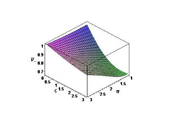
Refer to caption
Figure 1: (Coloronline) The smallest symplectic eigen value ν~subscript~𝜈\tilde{\nu}_{-} is plotted versus the dimensionless parameters η=αβ𝜂𝛼𝛽\eta=\frac{\alpha}{\beta} and ζ=p02β𝜁superscriptsubscript𝑝02𝛽\zeta=\frac{p_{0}^{2}}{\beta}.

In Fig.1 we plot ν~subscript~𝜈\tilde{\nu}_{-} versus the two parameters η=αβ𝜂𝛼𝛽\eta=\frac{\alpha}{\beta} and ζ=p02β𝜁superscriptsubscript𝑝02𝛽\zeta=\frac{p_{0}^{2}}{\beta}. From the graph it is clear that the two-particle state is separable ν~=1subscript~𝜈1\tilde{\nu}_{-}=1 when p0=0subscript𝑝00p_{0}=0 and α=β𝛼𝛽\alpha=\beta. As expected, the state is entangled for all other values of these parameters.

III.2 Single particle on a non-commutative plane

Let us now inspect the wave function given by Eq.(37) for any possible role of the underlying non-commutativity on its separability property. A single particle in two-dimensions can also be viewed (if the issue of statistics is disregarded), as two particles (or modes) in one-dimension, so that the wave function (37) can be regarded as the direct product of two particles on a line. On the basis of this argument, we can study the separability or inseparability of the two-particle state described by the effective commutative variance matrix VC1superscriptsubscript𝑉𝐶1V_{C}^{1} in the para above Eq.(48) in Section IIB. Here our task is to find the smallest symplectic eigenvalue ν~subscript~𝜈\tilde{\nu}_{-} of the partially transposed state described by the transposed variance matrix (V~C1)superscriptsubscript~𝑉𝐶1(\tilde{V}_{C}^{1}) obtained again from the variance matrix VC1superscriptsubscript𝑉𝐶1V_{C}^{1} using the transformation (15). The smallest symplectic eigenvalue is found out to be 111, i.e., ν~=1subscript~𝜈1\tilde{\nu}_{-}=1, which does not depend on the non-commutative parameter θ𝜃\theta. Therefore, using the PPT criterion we can conclude that the two-mode state described by the variance matrix (43) is separable for any non-commutative parameter θ𝜃\theta, since as expected, non-commutativity does not play any role at the single-particle level.

III.3 Two particles moving on a two-dimensional commutative plane

Let us consider two particles moving on a two dimensional plane described by the wave functions

ψ1(p1)subscript𝜓1subscript𝑝1\displaystyle\psi_{1}(\vec{p}_{1}) =\displaystyle= 1(πα)12exp(p122αip1a),1superscript𝜋𝛼12superscriptsubscript𝑝122𝛼𝑖subscript𝑝1𝑎\displaystyle\frac{1}{(\pi\alpha)^{\frac{1}{2}}}\exp\left(-\frac{\vec{p}_{1}^{2}}{2\alpha}-i\vec{p}_{1}\cdot\vec{a}\right), (67)
ψ2(p2)subscript𝜓2subscript𝑝2\displaystyle\psi_{2}(\vec{p}_{2}) =\displaystyle= 1(πα)12exp(p222α+ip2a)1superscript𝜋𝛼12superscriptsubscript𝑝222𝛼𝑖subscript𝑝2𝑎\displaystyle\frac{1}{(\pi\alpha)^{\frac{1}{2}}}\exp\left(-\frac{\vec{p}_{2}^{2}}{2\alpha}+i\vec{p}_{2}\cdot\vec{a}\right) (68)

The composite wave function for the two particles is constructed to be

Ψ(p1,p2)=N2[ψ1(p1)ψ2(p2)+ψ2(p1)ψ1(p2)]Ψsubscript𝑝1subscript𝑝2subscript𝑁2delimited-[]tensor-productsubscript𝜓1subscript𝑝1subscript𝜓2subscript𝑝2tensor-productsubscript𝜓2subscript𝑝1subscript𝜓1subscript𝑝2\displaystyle\Psi(\vec{p_{1}},\vec{p_{2}})=N_{2}[\psi_{1}(\vec{p_{1}})\otimes\psi_{2}(\vec{p_{2}})+\psi_{2}(\vec{p_{1}})\otimes\psi_{1}(\vec{p_{2}})] (69)

where N22=12(1+exp(2α|a|2))superscriptsubscript𝑁221212𝛼superscript𝑎2N_{2}^{2}=\frac{1}{2(1+\exp(-2\alpha|\vec{a}|^{2}))} is the normalization constant.

The variance matrix can be written in the covariant form as

V(2)=(AijBijCijDijBjiEijDjiGijCijDijAijBijDjiGijBjiEij)8×8superscript𝑉2subscriptmatrixsubscript𝐴𝑖𝑗subscript𝐵𝑖𝑗subscript𝐶𝑖𝑗subscript𝐷𝑖𝑗subscript𝐵𝑗𝑖subscript𝐸𝑖𝑗subscript𝐷𝑗𝑖subscript𝐺𝑖𝑗subscript𝐶𝑖𝑗subscript𝐷𝑖𝑗subscript𝐴𝑖𝑗subscript𝐵𝑖𝑗subscript𝐷𝑗𝑖subscript𝐺𝑖𝑗subscript𝐵𝑗𝑖subscript𝐸𝑖𝑗88\displaystyle V^{(2)}=\left(\matrix{A_{ij}&B_{ij}&C_{ij}&D_{ij}\cr B_{ji}&E_{ij}&D_{ji}&G_{ij}\cr C_{ij}&D_{ij}&A_{ij}&B_{ij}\cr D_{ji}&G_{ij}&B_{ji}&E_{ij}}\right)_{8\times 8} (70)

where Aijsubscript𝐴𝑖𝑗A_{ij},Bijsubscript𝐵𝑖𝑗B_{ij},Cijsubscript𝐶𝑖𝑗C_{ij},Dijsubscript𝐷𝑖𝑗D_{ij},Eijsubscript𝐸𝑖𝑗E_{ij} and Gijsubscript𝐺𝑖𝑗G_{ij} are 2×2222\times 2 block matrices given by

Aijsubscript𝐴𝑖𝑗\displaystyle A_{ij} =\displaystyle= x^ix^jIΨ(x^iI)Ψ(x^jI)Ψsubscriptdelimited-⟨⟩tensor-productsubscript^𝑥𝑖subscript^𝑥𝑗𝐼Ψsubscriptdelimited-⟨⟩tensor-productsubscript^𝑥𝑖𝐼Ψsubscriptdelimited-⟨⟩tensor-productsubscript^𝑥𝑗𝐼Ψ\displaystyle\langle\hat{x}_{i}~{}\hat{x}_{j}\otimes I\rangle_{\Psi}-\langle(\hat{x}_{i}\otimes I)\rangle_{\Psi}\langle(\hat{x}_{j}\otimes I)\rangle_{\Psi}{} (71)
=\displaystyle= Ix^ix^jΨ(Ix^i)Ψ(Ix^j)Ψsubscriptdelimited-⟨⟩tensor-product𝐼subscript^𝑥𝑖subscript^𝑥𝑗Ψsubscriptdelimited-⟨⟩tensor-product𝐼subscript^𝑥𝑖Ψsubscriptdelimited-⟨⟩tensor-product𝐼subscript^𝑥𝑗Ψ\displaystyle\langle I\otimes\hat{x}_{i}~{}\hat{x}_{j}\rangle_{\Psi}-\langle(I\otimes\hat{x}_{i})\rangle_{\Psi}\langle(I\otimes\hat{x}_{j})\rangle_{\Psi}{}
=\displaystyle= N22[2aiaj+δijα+δijαexp(2α|a|2)],superscriptsubscript𝑁22delimited-[]2subscript𝑎𝑖subscript𝑎𝑗subscript𝛿𝑖𝑗𝛼subscript𝛿𝑖𝑗𝛼2𝛼superscript𝑎2\displaystyle N_{2}^{2}[2a_{i}a_{j}+\frac{\delta_{ij}}{\alpha}+\frac{\delta_{ij}}{\alpha}\exp(-2\alpha|\vec{a}|^{2})],
Bijsubscript𝐵𝑖𝑗\displaystyle B_{ij} =\displaystyle= ((x^ip^j+p^jx^i)2I)Ψ(x^iI)Ψp^jIΨsubscriptdelimited-⟨⟩tensor-productsubscript^𝑥𝑖subscript^𝑝𝑗subscript^𝑝𝑗subscript^𝑥𝑖2𝐼Ψsubscriptdelimited-⟨⟩tensor-productsubscript^𝑥𝑖𝐼Ψsubscriptdelimited-⟨⟩tensor-productsubscript^𝑝𝑗𝐼Ψ\displaystyle\langle(\frac{(\hat{x}_{i}\hat{p}_{j}+\hat{p}_{j}\hat{x}_{i})}{2}\otimes I)\rangle_{\Psi}-\langle(\hat{x}_{i}\otimes I)\rangle_{\Psi}\langle\hat{p}_{j}\otimes I\rangle_{\Psi}{} (72)
=\displaystyle= (I(x^ip^j+p^jx^i)2)Ψ(Ix^i)ΨIp^jΨsubscriptdelimited-⟨⟩tensor-product𝐼subscript^𝑥𝑖subscript^𝑝𝑗subscript^𝑝𝑗subscript^𝑥𝑖2Ψsubscriptdelimited-⟨⟩tensor-product𝐼subscript^𝑥𝑖Ψsubscriptdelimited-⟨⟩tensor-product𝐼subscript^𝑝𝑗Ψ\displaystyle\langle(I\otimes\frac{(\hat{x}_{i}\hat{p}_{j}+\hat{p}_{j}\hat{x}_{i})}{2})\rangle_{\Psi}-\langle(I\otimes\hat{x}_{i})\rangle_{\Psi}\langle I\otimes\hat{p}_{j}\rangle_{\Psi}{}
=\displaystyle= 0,0\displaystyle 0,
Cijsubscript𝐶𝑖𝑗\displaystyle C_{ij} =\displaystyle= x^ix^jΨ(x^iI)Ψ(Ix^j)Ψ=2N22aiaj,subscriptdelimited-⟨⟩tensor-productsubscript^𝑥𝑖subscript^𝑥𝑗Ψsubscriptdelimited-⟨⟩tensor-productsubscript^𝑥𝑖𝐼Ψsubscriptdelimited-⟨⟩tensor-product𝐼subscript^𝑥𝑗Ψ2superscriptsubscript𝑁22subscript𝑎𝑖subscript𝑎𝑗\displaystyle\langle\hat{x}_{i}\otimes\hat{x}_{j}\rangle_{\Psi}-\langle(\hat{x}_{i}\otimes I)\rangle_{\Psi}\langle(I\otimes\hat{x}_{j})\rangle_{\Psi}=-2N_{2}^{2}a_{i}a_{j}, (73)
Dijsubscript𝐷𝑖𝑗\displaystyle D_{ij} =\displaystyle= x^ip^j)Ψx^iI)ΨIp^jΨ=0,\displaystyle\langle\hat{x}_{i}\otimes\hat{p}_{j})\rangle_{\Psi}-\langle\hat{x}_{i}\otimes I)\rangle_{\Psi}\langle I\otimes\hat{p}_{j}\rangle_{\Psi}=0, (74)
Eijsubscript𝐸𝑖𝑗\displaystyle E_{ij} =\displaystyle= p^ip^jIΨp^iIΨp^jIΨ=Ip^ip^jΨIp^i)ΨIp^jΨ\displaystyle\langle\hat{p}_{i}\hat{p}_{j}\otimes I\rangle_{\Psi}-\langle\hat{p}_{i}\otimes I\rangle_{\Psi}\langle\hat{p}_{j}\otimes I\rangle_{\Psi}=\langle I\otimes\hat{p}_{i}\hat{p}_{j}\rangle_{\Psi}-\langle I\otimes\hat{p}_{i})\rangle_{\Psi}\langle I\otimes\hat{p}_{j}\rangle_{\Psi}{} (75)
=\displaystyle= N22[αδij+(αδij2aiajα2)exp(2α|a|2)],superscriptsubscript𝑁22delimited-[]𝛼subscript𝛿𝑖𝑗𝛼subscript𝛿𝑖𝑗2subscript𝑎𝑖subscript𝑎𝑗superscript𝛼22𝛼superscript𝑎2\displaystyle N_{2}^{2}[\alpha\delta_{ij}+(\alpha\delta_{ij}-2a_{i}a_{j}\alpha^{2})\exp(-2\alpha|\vec{a}|^{2})],
Gijsubscript𝐺𝑖𝑗\displaystyle G_{ij} =\displaystyle= p^ip^j)Ψp^iIΨIp^jΨ=2N22aiajα2exp(2α|a|2)\displaystyle\langle\hat{p}_{i}\otimes\hat{p}_{j})\rangle_{\Psi}-\langle\hat{p}_{i}\otimes I\rangle_{\Psi}\langle I\otimes\hat{p}_{j}\rangle_{\Psi}=2N_{2}^{2}a_{i}a_{j}\alpha^{2}\exp(-2\alpha|\vec{a}|^{2}) (76)

To simplify the calculations and without any loss of generality we can take a2=0subscript𝑎20a_{2}=0. The 2×2222\times 2 and 4×4444\times 4 submatrices whose determinants are invariant under symplectic transformation are as follows:

αa=βa=(A11B11B11E11)2×2,αb=βb=(A22B22B22E22)2×2,γa=(C11D11D11G11)2×2,formulae-sequencesubscript𝛼𝑎subscript𝛽𝑎subscriptmatrixsubscript𝐴11subscript𝐵11subscript𝐵11subscript𝐸1122subscript𝛼𝑏subscript𝛽𝑏subscriptmatrixsubscript𝐴22subscript𝐵22subscript𝐵22subscript𝐸2222subscript𝛾𝑎subscriptmatrixsubscript𝐶11subscript𝐷11subscript𝐷11subscript𝐺1122\displaystyle\alpha_{a}=\beta_{a}=\left(\matrix{A_{11}&B_{11}\cr B_{11}&E_{11}}\right)_{2\times 2},\alpha_{b}=\beta_{b}=\left(\matrix{A_{22}&B_{22}\cr B_{22}&E_{22}}\right)_{2\times 2},\gamma_{a}=\left(\matrix{C_{11}&D_{11}\cr D_{11}&G_{11}}\right)_{2\times 2},{}
γb=(C22D22D22G22)2×2,δa=(αaγaγaTβa)4×4,δb=(αbγbγbTβb)4×4formulae-sequencesubscript𝛾𝑏subscriptmatrixsubscript𝐶22subscript𝐷22subscript𝐷22subscript𝐺2222formulae-sequencesubscript𝛿𝑎subscriptmatrixsubscript𝛼𝑎subscript𝛾𝑎superscriptsubscript𝛾𝑎𝑇subscript𝛽𝑎44subscript𝛿𝑏subscriptmatrixsubscript𝛼𝑏subscript𝛾𝑏superscriptsubscript𝛾𝑏𝑇subscript𝛽𝑏44\displaystyle\gamma_{b}=\left(\matrix{C_{22}&D_{22}\cr D_{22}&G_{22}}\right)_{2\times 2},\delta_{a}=\left(\matrix{\alpha_{a}&\gamma_{a}\cr\gamma_{a}^{T}&\beta_{a}}\right)_{4\times 4},\delta_{b}=\left(\matrix{\alpha_{b}&\gamma_{b}\cr\gamma_{b}^{T}&\beta_{b}}\right)_{4\times 4} (77)

The matrix elements ga,gb,gc,gd,ma,mb,mc,mdsubscript𝑔𝑎subscript𝑔𝑏subscript𝑔𝑐subscript𝑔𝑑subscript𝑚𝑎subscript𝑚𝑏subscript𝑚𝑐subscript𝑚𝑑g_{a},g_{b},g_{c},g_{d},m_{a},m_{b},m_{c},m_{d} of the standard form of the matrix (52) are determined by the symplectic invariants det(αa)=det(βa)=ga2=gc2subscript𝛼𝑎subscript𝛽𝑎superscriptsubscript𝑔𝑎2superscriptsubscript𝑔𝑐2\det(\alpha_{a})=\det(\beta_{a})=g_{a}^{2}=g_{c}^{2}, det(αb)=det(βb)=gb2=gd2subscript𝛼𝑏subscript𝛽𝑏superscriptsubscript𝑔𝑏2superscriptsubscript𝑔𝑑2\det(\alpha_{b})=\det(\beta_{b})=g_{b}^{2}=g_{d}^{2}, det(γa)=mamcsubscript𝛾𝑎subscript𝑚𝑎subscript𝑚𝑐\det(\gamma_{a})=m_{a}m_{c}, det(γb)=mbmdsubscript𝛾𝑏subscript𝑚𝑏subscript𝑚𝑑\det(\gamma_{b})=m_{b}m_{d} and det(V)=det(δa).det(δb)formulae-sequence𝑉subscript𝛿𝑎subscript𝛿𝑏\det(V)=\det(\delta_{a}).\det(\delta_{b}).

Our task is to calculate the symplectic eigenvalues of the matrix V𝑉V. The eigenvalues of the matrix |2iΩV|2𝑖Ω𝑉|2i\Omega V| are invariant under the action of symplectic transformation on the matrix V𝑉V. Therefore, the symplectic eigenvalues νisubscript𝜈𝑖\nu_{i}’s can be expressed in terms of symplectic invariant quantities detαasubscript𝛼𝑎\alpha_{a}, detαbsubscript𝛼𝑏\alpha_{b}, detβasubscript𝛽𝑎\beta_{a}, detβbsubscript𝛽𝑏\beta_{b}, detγasubscript𝛾𝑎\gamma_{a}, detγbsubscript𝛾𝑏\gamma_{b}, detδasubscript𝛿𝑎\delta_{a}, detδbsubscript𝛿𝑏\delta_{b} and are given by

νxsubscript𝜈𝑥\displaystyle\nu_{x} =\displaystyle= ±2Δx(V)±2(Δx(V))24detδa,plus-or-minusplus-or-minus2subscriptΔ𝑥𝑉2superscriptsubscriptΔ𝑥𝑉24subscript𝛿𝑎\displaystyle\pm\sqrt{2\Delta_{x}(V)\pm 2\sqrt{(\Delta_{x}(V))^{2}-4\det\delta_{a}}}, (78)
νysubscript𝜈𝑦\displaystyle\nu_{y} =\displaystyle= ±2Δy(V)±2(Δy(V))24detδbplus-or-minusplus-or-minus2subscriptΔ𝑦𝑉2superscriptsubscriptΔ𝑦𝑉24subscript𝛿𝑏\displaystyle\pm\sqrt{2\Delta_{y}(V)\pm 2\sqrt{(\Delta_{y}(V))^{2}-4\det\delta_{b}}} (79)

where Δx(V)=detαa+detβa+2detγasubscriptΔ𝑥𝑉subscript𝛼𝑎subscript𝛽𝑎2subscript𝛾𝑎\Delta_{x}(V)=\det\alpha_{a}+\det\beta_{a}+2\det\gamma_{a} and Δy(V)=detαb+detβb+2detγbsubscriptΔ𝑦𝑉subscript𝛼𝑏subscript𝛽𝑏2subscript𝛾𝑏\Delta_{y}(V)=\det\alpha_{b}+\det\beta_{b}+2\det\gamma_{b}. The smallest symplectic eigenvalue for the commutative system is given by

νC=min(νxC,νyC)superscriptsubscript𝜈𝐶𝑚𝑖𝑛superscriptsubscript𝜈subscript𝑥𝐶superscriptsubscript𝜈subscript𝑦𝐶\nu_{-}^{C}=min(\nu_{x_{-}}^{C},\nu_{y_{-}}^{C}) (80)

where

νxCsuperscriptsubscript𝜈subscript𝑥𝐶\displaystyle\nu_{x_{-}}^{C} =\displaystyle= 2Δx(V)2(Δx(V))24detδa,2subscriptΔ𝑥𝑉2superscriptsubscriptΔ𝑥𝑉24subscript𝛿𝑎\displaystyle\sqrt{2\Delta_{x}(V)-2\sqrt{(\Delta_{x}(V))^{2}-4\det\delta_{a}}}, (81)
νyCsuperscriptsubscript𝜈subscript𝑦𝐶\displaystyle\nu_{y_{-}}^{C} =\displaystyle= 2Δy(V)2(Δy(V))24detδb2subscriptΔ𝑦𝑉2superscriptsubscriptΔ𝑦𝑉24subscript𝛿𝑏\displaystyle\sqrt{2\Delta_{y}(V)-2\sqrt{(\Delta_{y}(V))^{2}-4\det\delta_{b}}} (82)

After taking partial transpose of the variance matrix V(2)superscript𝑉2V^{(2)}, The smallest symplectic eigenvalue is given by

ν~C=min(ν~xC,ν~yC)superscriptsubscript~𝜈𝐶𝑚𝑖𝑛superscriptsubscript~𝜈subscript𝑥𝐶superscriptsubscript~𝜈subscript𝑦𝐶\displaystyle\tilde{\nu}_{-}^{C}=min(\tilde{\nu}_{x_{-}}^{C},\tilde{\nu}_{y_{-}}^{C}) (83)

where

ν~xCsuperscriptsubscript~𝜈subscript𝑥𝐶\displaystyle\tilde{\nu}_{x_{-}}^{C} =\displaystyle= 2(A11+C11)(E11G11)2subscript𝐴11subscript𝐶11subscript𝐸11subscript𝐺11\displaystyle 2\sqrt{(A_{11}+C_{11})(E_{11}-G_{11})}{} (84)
=\displaystyle= 1(1+exp(2αa12))(1+exp(2αa12))(1+(14αa12)exp(2αa12)),112𝛼superscriptsubscript𝑎1212𝛼superscriptsubscript𝑎12114𝛼superscriptsubscript𝑎12𝑒𝑥𝑝2𝛼superscriptsubscript𝑎12\displaystyle\frac{1}{(1+\exp(-2\alpha a_{1}^{2}))}\sqrt{(1+\exp(-2\alpha a_{1}^{2}))(1+(1-4\alpha a_{1}^{2})exp(-2\alpha a_{1}^{2}))},
ν~yCsuperscriptsubscript~𝜈subscript𝑦𝐶\displaystyle\tilde{\nu}_{y_{-}}^{C} =\displaystyle= 2A22E22=12subscript𝐴22subscript𝐸221\displaystyle 2\sqrt{A_{22}E_{22}}=1 (85)
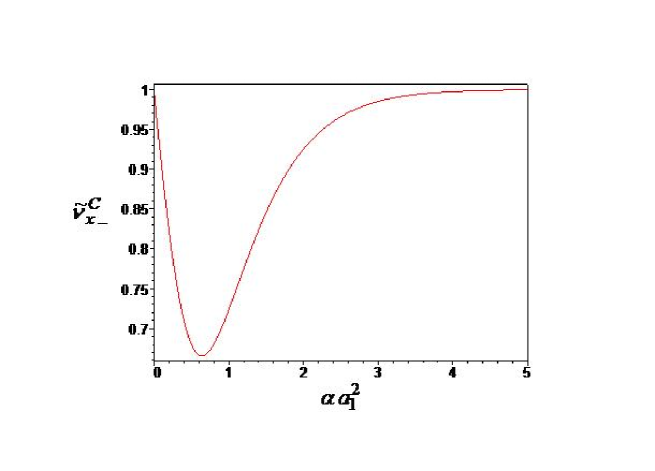
Refer to caption
Figure 2: (Coloronline) The symplectic eigenvalue ν~xCsuperscriptsubscript~𝜈subscript𝑥𝐶\tilde{\nu}_{x_{-}}^{C} is plotted versus αa12𝛼superscriptsubscript𝑎12\alpha a_{1}^{2}.

It is clear from Fig.2 that the smallest symplectic eigenvalue ν~Csuperscriptsubscript~𝜈𝐶\tilde{\nu}_{-}^{C} is less than 111 except at a1=0subscript𝑎10a_{1}=0 and a1subscript𝑎1a_{1}\rightarrow\infty. For these two cases the smallest symplectic eigenvalue takes the value 111 and hence the state Ψ(p)Ψ𝑝\Psi(\vec{p}) given in Eq. (69) is separable. For all other cases the state is entangled, as is evident also from the structure of the wave function in Eq.(69).

III.4 Two particles on a non-commutative plane

Let us finally consider the two particle state ΨΨ\Psi relevant to study the non-commutative dynamics on a two-dimensional plane:

Ψ=N(ψ1ψ2+F^θ2(ψ2ψ1))Ψ𝑁tensor-productsubscript𝜓1subscript𝜓2superscriptsubscript^𝐹𝜃2tensor-productsubscript𝜓2subscript𝜓1\displaystyle\Psi=N(\psi_{1}\otimes\psi_{2}+\hat{F}_{\theta}^{-2}(\psi_{2}\otimes\psi_{1})) (86)

where F^θ1=exp((iθij2)(p^ip^j))superscriptsubscript^𝐹𝜃1𝑖subscript𝜃𝑖𝑗2tensor-productsubscript^𝑝𝑖subscript^𝑝𝑗\hat{F}_{\theta}^{-1}=\exp\left((\frac{i\theta_{ij}}{2})(\hat{p}_{i}\otimes\hat{p}_{j})\right) is the (inverse) twist operator, as defined earlier in Section II, and N𝑁N is a normalization constant. ψ1subscript𝜓1\psi_{1} and ψ2subscript𝜓2\psi_{2} are given by

ψ1=ψ1(p;a,p0,α)=1παexp((12α)(pp02)2ipaiθijpip0j4)subscript𝜓1subscript𝜓1𝑝𝑎subscript𝑝0𝛼1𝜋𝛼12𝛼superscript𝑝subscript𝑝022𝑖𝑝𝑎𝑖subscript𝜃𝑖𝑗subscript𝑝𝑖subscript𝑝0𝑗4\displaystyle\psi_{1}=\psi_{1}(\vec{p};\vec{a},\vec{p}_{0},\alpha)=\frac{1}{\sqrt{\pi\alpha}}\exp((\frac{-1}{2\alpha})(\vec{p}-\frac{\vec{p}_{0}}{2})^{2}-i\vec{p}\cdot\vec{a}-\frac{i\theta_{ij}p_{i}p_{0j}}{4}) (87)

and ψ2=ψ1(p;a,p0,α)subscript𝜓2subscript𝜓1𝑝𝑎subscript𝑝0𝛼\psi_{2}=\psi_{1}(\vec{p};-\vec{a},-\vec{p}_{0},\alpha).

The variance matrix can be obtained after a long but straightforward computation (see Appendix II and III) in the covariant form and is given by

V¯=(A¯ijB¯ijC¯ijD¯ijB¯jiE¯ijD¯jiG¯ijC¯ijD¯ijA¯ijB¯ijD¯jiG¯ijB¯jiE¯ij)8×8¯𝑉subscriptmatrixsubscript¯𝐴𝑖𝑗subscript¯𝐵𝑖𝑗subscript¯𝐶𝑖𝑗subscript¯𝐷𝑖𝑗subscript¯𝐵𝑗𝑖subscript¯𝐸𝑖𝑗subscript¯𝐷𝑗𝑖subscript¯𝐺𝑖𝑗subscript¯𝐶𝑖𝑗subscript¯𝐷𝑖𝑗subscript¯𝐴𝑖𝑗subscript¯𝐵𝑖𝑗subscript¯𝐷𝑗𝑖subscript¯𝐺𝑖𝑗subscript¯𝐵𝑗𝑖subscript¯𝐸𝑖𝑗88\displaystyle\bar{V}=\left(\matrix{\bar{A}_{ij}&\bar{B}_{ij}&\bar{C}_{ij}&\bar{D}_{ij}\cr\bar{B}_{ji}&\bar{E}_{ij}&\bar{D}_{ji}&\bar{G}_{ij}\cr\bar{C}_{ij}&\bar{D}_{ij}&\bar{A}_{ij}&\bar{B}_{ij}\cr\bar{D}_{ji}&\bar{G}_{ij}&\bar{B}_{ji}&\bar{E}_{ij}}\right)_{8\times 8} (88)

in the basis ξ=(x¯1(1),x¯2(1),p1(1),p2(1),x¯1(2),x¯2(2),p1(2),p2(2))𝜉superscriptsubscript¯𝑥11superscriptsubscript¯𝑥21superscriptsubscript𝑝11superscriptsubscript𝑝21superscriptsubscript¯𝑥12superscriptsubscript¯𝑥22superscriptsubscript𝑝12superscriptsubscript𝑝22\vec{\xi}=(\bar{x}_{1}^{(1)},\bar{x}_{2}^{(1)},p_{1}^{(1)},p_{2}^{(1)},\bar{x}_{1}^{(2)},\bar{x}_{2}^{(2)},p_{1}^{(2)},p_{2}^{(2)}), where A¯ijsubscript¯𝐴𝑖𝑗\bar{A}_{ij}, B¯ijsubscript¯𝐵𝑖𝑗\bar{B}_{ij}, C¯ijsubscript¯𝐶𝑖𝑗\bar{C}_{ij}, D¯ijsubscript¯𝐷𝑖𝑗\bar{D}_{ij}, E¯ijsubscript¯𝐸𝑖𝑗\bar{E}_{ij} and G¯ijsubscript¯𝐺𝑖𝑗\bar{G}_{ij} are 2×2222\times 2 block matrices whose explicit forms are given in Appendix II.

In order to investigate the presence of entanglement in the two-particle state ΨΨ\Psi, described by the variance matrix (88), we have to again use the transformation (34) which transforms the variance matrix for the state in the non-commutative plane to the effective variance matrix (corresponding to the variance of commutative observables) in the commutative plane. Thereafter, we can apply the partial transposition to detect the entanglement in the state ΨΨ\Psi using the PPT criterion. Now, the transformed variance matrix in the commutative plane is given by

V=(AijBijCijDijBjiEijDjiGijCijDijAijBijDjiGijBjiEij)8×8𝑉subscriptmatrixsubscript𝐴𝑖𝑗subscript𝐵𝑖𝑗subscript𝐶𝑖𝑗subscript𝐷𝑖𝑗subscript𝐵𝑗𝑖subscript𝐸𝑖𝑗subscript𝐷𝑗𝑖subscript𝐺𝑖𝑗subscript𝐶𝑖𝑗subscript𝐷𝑖𝑗subscript𝐴𝑖𝑗subscript𝐵𝑖𝑗subscript𝐷𝑗𝑖subscript𝐺𝑖𝑗subscript𝐵𝑗𝑖subscript𝐸𝑖𝑗88\displaystyle V=\left(\matrix{A_{ij}&B_{ij}&C_{ij}&D_{ij}\cr B_{ji}&E_{ij}&D_{ji}&G_{ij}\cr C_{ij}&D_{ij}&A_{ij}&B_{ij}\cr D_{ji}&G_{ij}&B_{ji}&E_{ij}}\right)_{8\times 8} (89)

where Aijsubscript𝐴𝑖𝑗A_{ij}, Bijsubscript𝐵𝑖𝑗B_{ij}, Cijsubscript𝐶𝑖𝑗C_{ij}, Dijsubscript𝐷𝑖𝑗D_{ij}, Eijsubscript𝐸𝑖𝑗E_{ij} and Gijsubscript𝐺𝑖𝑗G_{ij} are 2×2222\times 2 block matrices related to the earlier (barred) matrices as follows:

Aij=A¯ij+θ2(ϵjkB¯ik+ϵikB¯jk)+θ24ϵikϵjlE¯klsubscript𝐴𝑖𝑗subscript¯𝐴𝑖𝑗𝜃2subscriptitalic-ϵ𝑗𝑘subscript¯𝐵𝑖𝑘subscriptitalic-ϵ𝑖𝑘subscript¯𝐵𝑗𝑘superscript𝜃24subscriptitalic-ϵ𝑖𝑘subscriptitalic-ϵ𝑗𝑙subscript¯𝐸𝑘𝑙\displaystyle A_{ij}=\bar{A}_{ij}+\frac{\theta}{2}(\epsilon_{jk}\bar{B}_{ik}+\epsilon_{ik}\bar{B}_{jk})+\frac{\theta^{2}}{4}\epsilon_{ik}\epsilon_{jl}\bar{E}_{kl} (90)
Bij=B¯ij+θ2ϵikE¯kjsubscript𝐵𝑖𝑗subscript¯𝐵𝑖𝑗𝜃2subscriptitalic-ϵ𝑖𝑘subscript¯𝐸𝑘𝑗\displaystyle B_{ij}=\bar{B}_{ij}+\frac{\theta}{2}\epsilon_{ik}\bar{E}_{kj} (91)
Cij=C¯ij+θ2(ϵjkD¯ik+ϵikD¯kj)+θ24ϵikϵjlG¯klsubscript𝐶𝑖𝑗subscript¯𝐶𝑖𝑗𝜃2subscriptitalic-ϵ𝑗𝑘subscript¯𝐷𝑖𝑘subscriptitalic-ϵ𝑖𝑘subscript¯𝐷𝑘𝑗superscript𝜃24subscriptitalic-ϵ𝑖𝑘subscriptitalic-ϵ𝑗𝑙subscript¯𝐺𝑘𝑙\displaystyle C_{ij}=\bar{C}_{ij}+\frac{\theta}{2}(\epsilon_{jk}\bar{D}_{ik}+\epsilon_{ik}\bar{D}_{kj})+\frac{\theta^{2}}{4}\epsilon_{ik}\epsilon_{jl}\bar{G}_{kl} (92)
Dij=D¯ij+θ2ϵikG¯kjsubscript𝐷𝑖𝑗subscript¯𝐷𝑖𝑗𝜃2subscriptitalic-ϵ𝑖𝑘subscript¯𝐺𝑘𝑗\displaystyle D_{ij}=\bar{D}_{ij}+\frac{\theta}{2}\epsilon_{ik}\bar{G}_{kj} (93)
Gij=G¯ijsubscript𝐺𝑖𝑗subscript¯𝐺𝑖𝑗\displaystyle G_{ij}=\bar{G}_{ij} (94)
Eij=E¯ijsubscript𝐸𝑖𝑗subscript¯𝐸𝑖𝑗\displaystyle E_{ij}=\bar{E}_{ij} (95)

We first determine the physicality condition for the variance matrix (89), and then perform the partial transposition of it. Finally, we compute its symplectic eigenvalues. For a straightforward illustration of the effect of non-commutativity on entanglement, let us consider the following case. We assume that the two particles described by the wave functions ψ1subscript𝜓1\psi_{1} and ψ2subscript𝜓2\psi_{2} are in a static position with respect to each other, i.e., p0=0subscript𝑝00\vec{p}_{0}=0 and that one of the components of b𝑏\vec{b} (defined as bi=ai+θijp0j=aisubscript𝑏𝑖subscript𝑎𝑖subscript𝜃𝑖𝑗subscript𝑝0𝑗subscript𝑎𝑖b_{i}=a_{i}+\theta_{ij}p_{0j}=a_{i}) is zero, (say, b2=0subscript𝑏20b_{2}=0). With the above assumptions, the symplectic eigenvalues νxNCsuperscriptsubscript𝜈subscript𝑥𝑁𝐶\nu_{x_{-}}^{NC} and νyNCsuperscriptsubscript𝜈subscript𝑦𝑁𝐶\nu_{y_{-}}^{NC} are obtained to be

νxNCsuperscriptsubscript𝜈subscript𝑥𝑁𝐶\displaystyle\nu_{x_{-}}^{NC} =\displaystyle= 2(A11C11)(E11G11)=2((A¯11C¯11)+θ24(E¯22G¯22))(E¯11G¯11)2subscript𝐴11subscript𝐶11subscript𝐸11subscript𝐺112subscript¯𝐴11subscript¯𝐶11superscript𝜃24subscript¯𝐸22subscript¯𝐺22subscript¯𝐸11subscript¯𝐺11\displaystyle 2\sqrt{(A_{11}-C_{11})(E_{11}-G_{11})}=2\sqrt{((\bar{A}_{11}-\bar{C}_{11})+\frac{\theta^{2}}{4}(\bar{E}_{22}-\bar{G}_{22}))(\bar{E}_{11}-\bar{G}_{11})}{} (96)
=\displaystyle= 2N21+3θ2α24+4b12α+4(3α2θ2+4)exp(8αb12(α2θ2+4))(α2θ2+4)2×\displaystyle 2N^{2}\sqrt{1+\frac{3\theta^{2}\alpha^{2}}{4}+4b_{1}^{2}\alpha+\frac{4(3\alpha^{2}\theta^{2}+4)\exp(\frac{-8\alpha b_{1}^{2}}{(\alpha^{2}\theta^{2}+4)})}{(\alpha^{2}\theta^{2}+4)^{2}}}\times{}
1+16exp(8αb12(α2θ2+4))(α2θ2+4)3(θ2α216αb12+4),1168𝛼superscriptsubscript𝑏12superscript𝛼2superscript𝜃24superscriptsuperscript𝛼2superscript𝜃243superscript𝜃2superscript𝛼216𝛼superscriptsubscript𝑏124\displaystyle\sqrt{1+\frac{16\exp(\frac{-8\alpha b_{1}^{2}}{(\alpha^{2}\theta^{2}+4)})}{(\alpha^{2}\theta^{2}+4)^{3}}(\theta^{2}\alpha^{2}-16\alpha b_{1}^{2}+4)},
νyNCsuperscriptsubscript𝜈subscript𝑦𝑁𝐶\displaystyle\nu_{y_{-}}^{NC} =\displaystyle= 2(A22C22)(E22G22)=2(A¯22C¯22+θ24(E¯11G¯11))(E¯22G¯22)2subscript𝐴22subscript𝐶22subscript𝐸22subscript𝐺222subscript¯𝐴22subscript¯𝐶22superscript𝜃24subscript¯𝐸11subscript¯𝐺11subscript¯𝐸22subscript¯𝐺22\displaystyle 2\sqrt{(A_{22}-C_{22})(E_{22}-G_{22})}=2\sqrt{(\bar{A}_{22}-\bar{C}_{22}+\frac{\theta^{2}}{4}(\bar{E}_{11}-\bar{G}_{11}))(\bar{E}_{22}-\bar{G}_{22})}{} (97)
=\displaystyle= 2N21+3θ2α24+4exp(8αb12(α2θ2+4))(α2θ2+4)3(3θ4α4+16α2θ2+1632θ2α3b12)×\displaystyle 2N^{2}\sqrt{1+\frac{3\theta^{2}\alpha^{2}}{4}+\frac{4\exp(\frac{-8\alpha b_{1}^{2}}{(\alpha^{2}\theta^{2}+4)})}{(\alpha^{2}\theta^{2}+4)^{3}}(3\theta^{4}\alpha^{4}+16\alpha^{2}\theta^{2}+16-32\theta^{2}\alpha^{3}b_{1}^{2})}\times{}
1+16exp(8αb12(α2θ2+4))(α2θ2+4)21168𝛼superscriptsubscript𝑏12superscript𝛼2superscript𝜃24superscriptsuperscript𝛼2superscript𝜃242\displaystyle\sqrt{1+\frac{16\exp(\frac{-8\alpha b_{1}^{2}}{(\alpha^{2}\theta^{2}+4)})}{(\alpha^{2}\theta^{2}+4)^{2}}}

The variance matrix (89) represents the physical state if it satisfies the appropriate physicality condition for a non-commutative system explained in section IIC, viz.

(νNC)2=min((νxNC)2,(νyNC)2)(νNC(θ))min2superscriptsuperscriptsubscript𝜈𝑁𝐶2𝑚𝑖𝑛superscriptsuperscriptsubscript𝜈subscript𝑥𝑁𝐶2superscriptsuperscriptsubscript𝜈subscript𝑦𝑁𝐶2subscriptsuperscriptsuperscriptsubscript𝜈𝑁𝐶𝜃2𝑚𝑖𝑛\displaystyle(\nu_{-}^{NC})^{2}=min((\nu_{x_{-}}^{NC})^{2},(\nu_{y_{-}}^{NC})^{2})\geq(\nu_{-}^{NC}(\theta))^{2}_{min} (98)

In order to extract the θ𝜃\theta-dependence in the physicality condition, we have to first obtain the minimum uncertainty state for which the function Δx^1Δx^2(θ)Δsubscript^𝑥1Δsubscript^𝑥2𝜃\Delta\hat{x}_{1}\Delta\hat{x}_{2}(\theta) is minimized. The above function can be read off from the elements of the effective commutative variance matrix (89), and is given by A11A22subscript𝐴11subscript𝐴22A_{11}A_{22} in terms of parameters defined in Eq.(90). Note that (νNC(θ))minsubscriptsuperscriptsubscript𝜈𝑁𝐶𝜃𝑚𝑖𝑛(\nu_{-}^{NC}(\theta))_{min} depends also on the state parameters α𝛼\alpha and b1subscript𝑏1b_{1}. For the present computation we minimize Δx^1Δx^2(θ)Δsubscript^𝑥1Δsubscript^𝑥2𝜃\Delta\hat{x}_{1}\Delta\hat{x}_{2}(\theta) with respect to the spread α𝛼\alpha for various values of the particle separation a1=b1subscript𝑎1subscript𝑏1a_{1}=b_{1}. Or in other words, choosing a particular state corresponding to a specific value of b1subscript𝑏1b_{1}, we compute the value of α𝛼\alpha (say, αminsubscript𝛼𝑚𝑖𝑛\alpha_{min}) for which the uncertainty Δx^1Δx^2(θ)Δsubscript^𝑥1Δsubscript^𝑥2𝜃\Delta\hat{x}_{1}\Delta\hat{x}_{2}(\theta) is minimized. Next, we find the minimum symplectic eigenvalue (νNC(θ))minsubscriptsuperscriptsubscript𝜈𝑁𝐶𝜃𝑚𝑖𝑛(\nu_{-}^{NC}(\theta))_{min} by substituting the values of αminsubscript𝛼𝑚𝑖𝑛\alpha_{min} and b1subscript𝑏1b_{1} in Eqs.(96) and (97). We then repeat this computation for other values of b1subscript𝑏1b_{1}. We find that the value of αminsubscript𝛼𝑚𝑖𝑛\alpha_{min} minimizing the position-position uncertainty stays constant for a specific range of the parameter b1subscript𝑏1b_{1}, and then again acquires a different contant value for another range of b1subscript𝑏1b_{1}. In this way we obtain the physicality condition for ranges of states parametrized by various values of particle separation b1subscript𝑏1b_{1}. The values of (νNC(θ))minsubscriptsuperscriptsubscript𝜈𝑁𝐶𝜃𝑚𝑖𝑛(\nu_{-}^{NC}(\theta))_{min} corresponding to three different ranges of values for the parameter b1subscript𝑏1b_{1} are plotted in Figs.3, 4 and 5, with the respective minimum uncertainty conditions, i.e., αmin1.4/θsimilar-to-or-equalssubscript𝛼𝑚𝑖𝑛1.4𝜃\alpha_{min}\simeq 1.4/\theta, αmin1.6/θsimilar-to-or-equalssubscript𝛼𝑚𝑖𝑛1.6𝜃\alpha_{min}\simeq 1.6/\theta and αmin1.8/θsimilar-to-or-equalssubscript𝛼𝑚𝑖𝑛1.8𝜃\alpha_{min}\simeq 1.8/\theta displayed respectively on the figures.
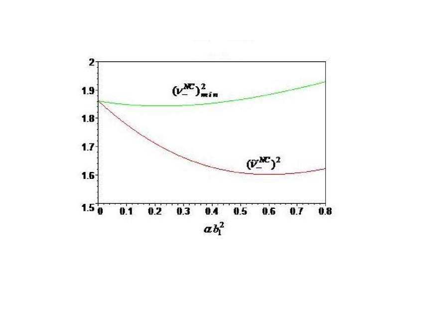
Refer to caption
Figure 3: (Coloronline) The smallest symplectic eigenvalue (ν~xNC)2superscriptsuperscriptsubscript~𝜈subscript𝑥𝑁𝐶2(\tilde{\nu}_{x_{-}}^{NC})^{2} of the partially transformed variance matrix V~~𝑉\tilde{V} and the function (νNC(θ))minsubscriptsuperscriptsubscript𝜈𝑁𝐶𝜃𝑚𝑖𝑛(\nu_{-}^{NC}(\theta))_{min} representing the entanglement criterion are plotted versus αb12𝛼superscriptsubscript𝑏12\alpha b_{1}^{2}. Here αmin1.4/θsimilar-to-or-equalssubscript𝛼𝑚𝑖𝑛1.4𝜃\alpha_{min}\simeq 1.4/\theta. The state is entangled since (ν~xNC)2<(νNC(θ))min2superscriptsuperscriptsubscript~𝜈subscript𝑥𝑁𝐶2subscriptsuperscriptsuperscriptsubscript𝜈𝑁𝐶𝜃2𝑚𝑖𝑛(\tilde{\nu}_{x_{-}}^{NC})^{2}<(\nu_{-}^{NC}(\theta))^{2}_{min} for all values in the parameter space.
Refer to caption
Figure 4: (Coloronline) The smallest symplectic eigenvalue (ν~xNC)2superscriptsuperscriptsubscript~𝜈subscript𝑥𝑁𝐶2(\tilde{\nu}_{x_{-}}^{NC})^{2} of the partially transformed variance matrix V~~𝑉\tilde{V} and the function (νNC(θ))minsubscriptsuperscriptsubscript𝜈𝑁𝐶𝜃𝑚𝑖𝑛(\nu_{-}^{NC}(\theta))_{min} representing the entanglement criterion are plotted versus αb12𝛼superscriptsubscript𝑏12\alpha b_{1}^{2}. Here αmin1.6/θsimilar-to-or-equalssubscript𝛼𝑚𝑖𝑛1.6𝜃\alpha_{min}\simeq 1.6/\theta. The state is entangled since (ν~xNC)2<(νNC(θ))min2superscriptsuperscriptsubscript~𝜈subscript𝑥𝑁𝐶2subscriptsuperscriptsuperscriptsubscript𝜈𝑁𝐶𝜃2𝑚𝑖𝑛(\tilde{\nu}_{x_{-}}^{NC})^{2}<(\nu_{-}^{NC}(\theta))^{2}_{min} for all values in the parameter space.
Refer to caption
Figure 5: (Coloronline) The smallest symplectic eigenvalue (ν~xNC)2superscriptsuperscriptsubscript~𝜈subscript𝑥𝑁𝐶2(\tilde{\nu}_{x_{-}}^{NC})^{2} of the partially transformed variance matrix V~~𝑉\tilde{V} and the function (νNC(θ))minsubscriptsuperscriptsubscript𝜈𝑁𝐶𝜃𝑚𝑖𝑛(\nu_{-}^{NC}(\theta))_{min} representing the entanglement criterion are plotted versus αb12𝛼superscriptsubscript𝑏12\alpha b_{1}^{2}. Here αmin1.8/θsimilar-to-or-equalssubscript𝛼𝑚𝑖𝑛1.8𝜃\alpha_{min}\simeq 1.8/\theta. The state is entangled since (ν~xNC)2<(νNC(θ))min2superscriptsuperscriptsubscript~𝜈subscript𝑥𝑁𝐶2subscriptsuperscriptsuperscriptsubscript𝜈𝑁𝐶𝜃2𝑚𝑖𝑛(\tilde{\nu}_{x_{-}}^{NC})^{2}<(\nu_{-}^{NC}(\theta))^{2}_{min} for all values in the parameter space.

Next, in order to apply the PPT entanglement criterion, we perform partial transposition of the variance matrix, which corresponds to time reversal, or in terms of continuous variables, sign change of momentum variables. Thus, when we take the partial transpose, we have to change the sign of all the components of the momentum variables of one of the particles. Therefore, the variance matrix V𝑉V transforms under partial transposition as

VV~=ΛVΛ𝑉~𝑉Λ𝑉Λ\displaystyle V\rightarrow\tilde{V}=\Lambda V\Lambda (99)

where Λ=diag(1,1,1,1,1,1,1,1)Λ𝑑𝑖𝑎𝑔11111111\Lambda=diag(1,1,1,1,1,1,-1,-1). After performing partial transposition operation, we compute the eigenvalues ν~subscript~𝜈\tilde{\nu}_{-} of the matrix |2iΩV~|2𝑖Ω~𝑉|2i\Omega\tilde{V}|. Due to the partial transposition operation, the symplectic invariant quantities detγa𝑑𝑒𝑡subscript𝛾𝑎det\gamma_{a} and detγb𝑑𝑒𝑡subscript𝛾𝑏det\gamma_{b} just flip their sign. Hence, the expression for the smallest symplectic eigenvalue can be written as

ν~NC=min(ν~xNC,ν~yNC)superscriptsubscript~𝜈𝑁𝐶𝑚𝑖𝑛superscriptsubscript~𝜈subscript𝑥𝑁𝐶superscriptsubscript~𝜈subscript𝑦𝑁𝐶\displaystyle\tilde{\nu}_{-}^{NC}=min(\tilde{\nu}_{x_{-}}^{NC},\tilde{\nu}_{y_{-}}^{NC}) (100)

where

ν~xNCsuperscriptsubscript~𝜈subscript𝑥𝑁𝐶\displaystyle\tilde{\nu}_{x_{-}}^{NC} =\displaystyle= 2Δx(V~)2(Δx(V~))24detδa,Δx(V~)=detαa+detβa2detγa,2subscriptΔ𝑥~𝑉2superscriptsubscriptΔ𝑥~𝑉24subscript𝛿𝑎subscriptΔ𝑥~𝑉subscript𝛼𝑎subscript𝛽𝑎2subscript𝛾𝑎\displaystyle\sqrt{2\Delta_{x}(\tilde{V})-2\sqrt{(\Delta_{x}(\tilde{V}))^{2}-4\det\delta_{a}}},\quad\Delta_{x}(\tilde{V})=\det\alpha_{a}+\det\beta_{a}-2\det\gamma_{a}, (101)
ν~yNCsuperscriptsubscript~𝜈subscript𝑦𝑁𝐶\displaystyle\tilde{\nu}_{y_{-}}^{NC} =\displaystyle= 2Δy(V~)2(Δy(V~))24detδb,Δy(V~)=detαb+detβb2detγb2subscriptΔ𝑦~𝑉2superscriptsubscriptΔ𝑦~𝑉24subscript𝛿𝑏subscriptΔ𝑦~𝑉subscript𝛼𝑏subscript𝛽𝑏2subscript𝛾𝑏\displaystyle\sqrt{2\Delta_{y}(\tilde{V})-2\sqrt{(\Delta_{y}(\tilde{V}))^{2}-4\det\delta_{b}}},\quad\Delta_{y}(\tilde{V})=\det\alpha_{b}+\det\beta_{b}-2\det\gamma_{b} (102)

For a non-commutative system the state is entangled when the smallest symplectic eigenvalue ν~ν~NCsubscript~𝜈superscriptsubscript~𝜈𝑁𝐶\tilde{\nu}_{-}\equiv\tilde{\nu}_{-}^{NC} given in Eq.(100) satisfies the condition (following from Eq.(59))

(ν~NC)2<(νNC(θ))min2superscriptsuperscript~subscript𝜈𝑁𝐶2subscriptsuperscriptsuperscriptsubscript𝜈𝑁𝐶𝜃2𝑚𝑖𝑛\displaystyle(\tilde{\nu_{-}}^{NC})^{2}<(\nu_{-}^{NC}(\theta))^{2}_{min} (103)

We now perform the partial transposition of the variance matrix (89) and compute the symplectic eigenvalues ν~xNCsuperscriptsubscript~𝜈subscript𝑥𝑁𝐶\tilde{\nu}_{x_{-}}^{NC} and ν~yNCsuperscriptsubscript~𝜈subscript𝑦𝑁𝐶\tilde{\nu}_{y_{-}}^{NC} of the partially transposed matrix with the help of Eqs.(101) and (102). These are given by

(ν~xNC)2superscriptsuperscriptsubscript~𝜈subscript𝑥𝑁𝐶2\displaystyle(\tilde{\nu}_{x_{-}}^{NC})^{2} =4N4[1+3θ2α24+4(8θ4α5b12+3θ4α4+16θ2α2+16)exp(8αb12(α2θ2+4))(α2θ2+4)3\displaystyle=4N^{4}[1+\frac{3\theta^{2}\alpha^{2}}{4}+\frac{4(8\theta^{4}\alpha^{5}b_{1}^{2}+3\theta^{4}\alpha^{4}+16\theta^{2}\alpha^{2}+16)exp(\frac{-8\alpha b_{1}^{2}}{(\alpha^{2}\theta^{2}+4)})}{(\alpha^{2}\theta^{2}+4)^{3}}{} (104)
256N2θ4α5b12exp(16αb12(α2θ2+4))(α2θ2+4)4][1+16(α2θ216αb12+4)exp(8αb12((α2θ2+4))(α2θ2+4)3],\displaystyle-\frac{256N^{2}\theta^{4}\alpha^{5}b_{1}^{2}exp(\frac{-16\alpha b_{1}^{2}}{(\alpha^{2}\theta^{2}+4)})}{(\alpha^{2}\theta^{2}+4)^{4}}][1+\frac{16(\alpha^{2}\theta^{2}-16\alpha b_{1}^{2}+4)exp(\frac{-8\alpha b_{1}^{2}}{((\alpha^{2}\theta^{2}+4)})}{(\alpha^{2}\theta^{2}+4)^{3}}],
(ν~yNC)2superscriptsuperscriptsubscript~𝜈subscript𝑦𝑁𝐶2\displaystyle(\tilde{\nu}_{y_{-}}^{NC})^{2} =4N4[1+3θ2α24+4(3θ2α2+4)exp(8αb12(α2θ2+4))(α2θ2+4)2][1+16exp(8αb12((α2θ2+4))(α2θ2+4)2]\displaystyle=4N^{4}[1+\frac{3\theta^{2}\alpha^{2}}{4}+\frac{4(3\theta^{2}\alpha^{2}+4)exp(\frac{-8\alpha b_{1}^{2}}{(\alpha^{2}\theta^{2}+4)})}{(\alpha^{2}\theta^{2}+4)^{2}}][1+\frac{16exp(\frac{-8\alpha b_{1}^{2}}{((\alpha^{2}\theta^{2}+4)})}{(\alpha^{2}\theta^{2}+4)^{2}}] (105)

where N2=12(1+4/5exp(8αb12/5))superscript𝑁2121458𝛼superscriptsubscript𝑏125N^{2}=\frac{1}{2(1+4/5\exp(-8\alpha b_{1}^{2}/5))}. The state is entangled if the smallest symplectic eigenvalue satisfies the condition (103).

The smallest symplectic eigenvalue (ν~xNC)2superscriptsuperscriptsubscript~𝜈subscript𝑥𝑁𝐶2(\tilde{\nu}_{x_{-}}^{NC})^{2} is plotted versus αb12𝛼superscriptsubscript𝑏12\alpha b_{1}^{2} in Figs. 3, 4 and 5 respectively for different ranges of the parameter b1subscript𝑏1b_{1} corresponding to the respective displayed values of αminsubscript𝛼𝑚𝑖𝑛\alpha_{min}. From the figures it can be seen that ν~xNCsuperscriptsubscript~𝜈subscript𝑥𝑁𝐶\tilde{\nu}_{x_{-}}^{NC} satisfies the condition (103), for a range of parameter values thus showing that the state is entangled for these parameter values.

Now we are in a position to compare the amount of entanglement in the commutative (i.e.,taking the θ=0𝜃0\theta=0 limit in the composite state ΨΨ\Psi of Eq.(53)) and non-commutative (i.e.,θ0𝜃0~{}\theta\neq 0) case, respectively. The respective magnitudes of entanglement can be quantified using the logarithmic negativitylogneg . The two expressions can be formally written as

ECsuperscript𝐸𝐶\displaystyle E^{C} =\displaystyle= max[0,12log2(ν~C)2],𝑚𝑎𝑥012𝑙𝑜subscript𝑔2superscriptsuperscriptsubscript~𝜈𝐶2\displaystyle max[0,-\frac{1}{2}log_{2}(\tilde{\nu}_{-}^{C})^{2}], (106)
ENCsuperscript𝐸𝑁𝐶\displaystyle E^{NC} =\displaystyle= max[0,12log2(ν~)2]𝑚𝑎𝑥012𝑙𝑜subscript𝑔2superscriptsubscript~𝜈2\displaystyle max[0,-\frac{1}{2}log_{2}(\tilde{\nu}_{-})^{2}] (107)

where ν~2=(ν~NC)2(νNC(θ))min2+1superscriptsubscript~𝜈2superscriptsuperscriptsubscript~𝜈𝑁𝐶2superscriptsubscriptsuperscriptsubscript𝜈𝑁𝐶𝜃𝑚𝑖𝑛21\tilde{\nu}_{-}^{2}=(\tilde{\nu}_{-}^{NC})^{2}-(\nu_{-}^{NC}(\theta))_{min}^{2}+1, and the smallest symplectic eigenvalues ν~Csuperscriptsubscript~𝜈𝐶\tilde{\nu}_{-}^{C} and ν~NCsuperscriptsubscript~𝜈𝑁𝐶\tilde{\nu}_{-}^{NC} are obtained from Eqs.(83) and (100), respectively.
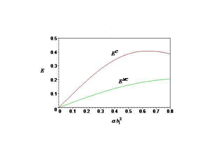
Refer to caption
Figure 6: (Coloronline) The logarithmic negativity ECsuperscript𝐸𝐶E^{C} and ENCsuperscript𝐸𝑁𝐶E^{NC} are plotted versus αb12𝛼superscriptsubscript𝑏12\alpha b_{1}^{2} respectively for the commutative and non-commutative systems. Here αmin1.4/θsimilar-to-or-equalssubscript𝛼𝑚𝑖𝑛1.4𝜃\alpha_{min}\simeq 1.4/\theta.
Refer to caption
Figure 7: (Coloronline) The logarithmic negativity ECsuperscript𝐸𝐶E^{C} and ENCsuperscript𝐸𝑁𝐶E^{NC} are plotted versus αb12𝛼superscriptsubscript𝑏12\alpha b_{1}^{2} respectively for the commutative and non-commutative systems. Here αmin1.6/θsimilar-to-or-equalssubscript𝛼𝑚𝑖𝑛1.6𝜃\alpha_{min}\simeq 1.6/\theta.
Refer to caption
Figure 8: (Coloronline) The logarithmic negativity ECsuperscript𝐸𝐶E^{C} and ENCsuperscript𝐸𝑁𝐶E^{NC} are plotted versus αb12𝛼superscriptsubscript𝑏12\alpha b_{1}^{2} respectively for the commutative and non-commutative systems. Here αmin1.8/θsimilar-to-or-equalssubscript𝛼𝑚𝑖𝑛1.8𝜃\alpha_{min}\simeq 1.8/\theta.

In Figs. 6, 7 and 8 the magnitude of entanglement E𝐸E is plotted versus αb12𝛼superscriptsubscript𝑏12\alpha b_{1}^{2} respectively for different ranges of b1subscript𝑏1b_{1} (corresponding to the appropriate values of αminsubscript𝛼𝑚𝑖𝑛\alpha_{min} for the respective ranges of b1subscript𝑏1b_{1}) for the commutative as well as the non-commutative case separately. One can see that the underlying non-commutativity leads to a reduction of entanglement in all the cases. This feature is most prominent, i.e., the difference in the magnitute of entanglement between the commutative and the non-commutative system is maximum, when αb12O(1)similar-to𝛼superscriptsubscript𝑏12𝑂1\alpha b_{1}^{2}\sim O(1). For larger separation of the two particles (b1=a1subscript𝑏1subscript𝑎1b_{1}=a_{1} for the case we have studied), this difference tends to decrease, and the state becomes separable for asymptotically large values of b1subscript𝑏1b_{1} in the commutative as well as the non-commutative case. This clear manifestation of non-commutativity hindering the entanglement of two particles at small distances, could presumably be correlated to the enhanced variances of the physical observables coming from the modified space-space and phase-space uncertainty relations (45) and (47) in non-commutative space.

IV Summary and Conclusions

In this paper we have investigated the role of position-space noncommutativity on the entanglement of bipartite systems. We focus on Gaussian states in the continuous variable position-momentum phase space, where the formalism for detecting and quantifying bipartite entanglement is well-established simon1 ; duan ; reviews . We have first extended the symplectic formalism for studying entanglement for a bipartite Gaussian state residing on a two- (spatial) dimensional plane. The validity of this formulation is illustrated with the help of an example of a two-particle state which is shown to exhibit expected entanglement properties. We then prescribe our formulation for extending the PPT criterion for entanglement of non-commutative systems. The θ𝜃\theta-dependence of the entanglement criterion is derived. As an off-shoot we show that for a single particle on the two-dimensional noncommutative plane, whose state may be viewed as a composite state of two one-dimensional modes, the underlying non-commutativity does not impact the a priori separability of the modes. We have finally presented an example of a non-commutative state of two particles. This represents a pure state and is manifestly entangled in the commutative (θ=0𝜃0\theta=0) limit. As a striking feature of our formalism, we are able to show that the magnitude of entanglement reduces under the effect of non-commutative dynamics for a whole range of physically allowed parameter values.

A notable consequence of this study has been our result of how the criterion of entanglement itself is modified in the presence of non-commutativity. Our goal in this paper has been not to regard entanglement as a resource for performing information processing tasks, but rather to study the impact of noncommutativity on entanglement itself. Indeed, the role of (anti-)symmetrization associated with the statistics of indistinguishable particles on their entanglement is itself not yet well-understood, and any entanglement resulting from such (anti-) symmetrization might not be amenable for use as resourceeckert . It may be relevant to observe here that quantum entanglement is difficult to preserve under the interactions of the system with the environment. Decoherencezurek is an effective phenomenon where one is practically unable to monitor the huge number of degrees of freedom of the environment. It remains an open question whether the loss (or reduction) of quantum coherence could be an intrinsic feature of the dynamics of individual systems, instead of being a purely effective one. There are indeed some models such as gravity induced state vector reductionpenrose and continuous spontaneous localizationcsl , that produce quantum decoherence as an ingredient of the basic quantum dynamics itself, though these schemes are yet to be verified experimentally. On the other hand, the idea of space-space noncommutativity is well-inspired at the fundamental level, and is certainly an off-shoot of the physics in strong gravitational fields in the presence of event horizons of black holesdfr . Non-commutative dynamics being able to restrict the entanglement of two particles at short distances is a remarkable consequence of the analysis presented in this paper. Such an effect of non-commutativity is expected to have interesting consequences on the entanglement of quantum states and related information capacities wherever position-space noncommutativity is effective.


Acknowledgments: We would like to thank Subhash Chaturvedi and Frederik G. Scholtz for discussions, and Soumen Mandal for help using Mathematica to compute the integrals for the non-commutative variance matrix elements. ASM would like to acknowledge support from a project funded by DST, India.

Appendix I: Standard form of the variance matrix

By the following steps one can bring a variance matrix into the standard form from which its symplectic eigen values could be easily obtained. Step-I: The variance matrix can be expressed in the basis (x1(1),p1(1),x2(1),p2(1),x1(2),p1(2),,x2(2),p2(2))(x_{1}^{(1)},p_{1}^{(1)},x_{2}^{(1)},p_{2}^{(1)},x_{1}^{(2)},p_{1}^{(2)},,x_{2}^{(2)},p_{2}^{(2)}) in terms of 2×2222\times 2 block matrices as:

V=(αx(1)αx,y(1)γx(1,2)γx,y(1,2)αx,y(1)αy(1)(γx,y(1,2))Tγy(1,2)(γx(1,2))Tγx,y(1,2)βx(2)βx,y(2)(γx,y(1,2))T(γy(1,2))Tβx,y(2)βy(2))8×8Vsubscriptmatrixsuperscriptsubscript𝛼𝑥1superscriptsubscript𝛼𝑥𝑦1superscriptsubscript𝛾𝑥12superscriptsubscript𝛾𝑥𝑦12superscriptsubscript𝛼𝑥𝑦1superscriptsubscript𝛼𝑦1superscriptsuperscriptsubscript𝛾𝑥𝑦12𝑇superscriptsubscript𝛾𝑦12superscriptsuperscriptsubscript𝛾𝑥12𝑇superscriptsubscript𝛾𝑥𝑦12superscriptsubscript𝛽𝑥2superscriptsubscript𝛽𝑥𝑦2superscriptsuperscriptsubscript𝛾𝑥𝑦12𝑇superscriptsuperscriptsubscript𝛾𝑦12𝑇superscriptsubscript𝛽𝑥𝑦2superscriptsubscript𝛽𝑦288\displaystyle\textsl{V}=\left(\matrix{\alpha_{x}^{(1)}&\alpha_{x,y}^{(1)}&\gamma_{x}^{(1,2)}&\gamma_{x,y}^{(1,2)}\cr\alpha_{x,y}^{(1)}&\alpha_{y}^{(1)}&(\gamma_{x,y}^{(1,2)})^{T}&\gamma_{y}^{(1,2)}\cr(\gamma_{x}^{(1,2)})^{T}&\gamma_{x,y}^{(1,2)}&\beta_{x}^{(2)}&\beta_{x,y}^{(2)}\cr(\gamma_{x,y}^{(1,2)})^{T}&(\gamma_{y}^{(1,2)})^{T}&\beta_{x,y}^{(2)}&\beta_{y}^{(2)}}\right)_{8\times 8} (108)

The superscripts 111 and 222 refer to the first and second particle, respectively, and subscripts x1subscript𝑥1x_{1} and x2subscript𝑥2x_{2} refer to the two perpendicular axes x𝑥x and y𝑦y, respectively. Using Williamson’s theorem william , we can choose two local symplectic transformations S1,S2Sp(4,R)subscript𝑆1subscript𝑆2𝑆𝑝4𝑅S_{1},S_{2}\in Sp(4,R) which transform

V(S1S2)V(S1TS2T)=V(gaI0(γx(1,2))(γx,y(1,2))0gbI((γx,y(1,2)))T(γy(1,2))((γx(1,2)))T(γx,y(1,2))gcI0((γx,y(1,2)))T((γy(1,2)))T0gdI)𝑉tensor-productsubscript𝑆1subscript𝑆2𝑉tensor-productsuperscriptsubscript𝑆1𝑇superscriptsubscript𝑆2𝑇superscript𝑉matrixsubscript𝑔𝑎𝐼0superscriptsuperscriptsubscript𝛾𝑥12superscriptsuperscriptsubscript𝛾𝑥𝑦120subscript𝑔𝑏𝐼superscriptsuperscriptsuperscriptsubscript𝛾𝑥𝑦12𝑇superscriptsuperscriptsubscript𝛾𝑦12superscriptsuperscriptsuperscriptsubscript𝛾𝑥12𝑇superscriptsuperscriptsubscript𝛾𝑥𝑦12subscript𝑔𝑐𝐼0superscriptsuperscriptsuperscriptsubscript𝛾𝑥𝑦12𝑇superscriptsuperscriptsuperscriptsubscript𝛾𝑦12𝑇0subscript𝑔𝑑𝐼\displaystyle V\rightarrow(S_{1}\otimes S_{2})V(S_{1}^{T}\otimes S_{2}^{T})=V^{\prime}\equiv\left(\matrix{g_{a}I&0&(\gamma_{x}^{(1,2)})^{\prime}&(\gamma_{x,y}^{(1,2)})^{\prime}\cr 0&g_{b}I&((\gamma_{x,y}^{(1,2)})^{\prime})^{T}&(\gamma_{y}^{(1,2)})^{\prime}\cr((\gamma_{x}^{(1,2)})^{\prime})^{T}&(\gamma_{x,y}^{(1,2)})^{\prime}&g_{c}I&0\cr((\gamma_{x,y}^{(1,2)})^{\prime})^{T}&((\gamma_{y}^{(1,2)})^{\prime})^{T}&0&g_{d}I}\right) (109)

where I𝐼I denotes the 2×2222\times 2 identity matrix and 00 denotes the 2×2222\times 2 null matrix. As a result of the transformation, the cross-correlation block matrices are modified, and they are denoted with prime.

Step-II: There exist symplectic transformations S3,S4Sp(2,R)subscript𝑆3subscript𝑆4𝑆𝑝2𝑅S_{3},S_{4}\in Sp(2,R) which transform the variance matrix Vsuperscript𝑉V^{\prime} as:

V(S30000S40000S30000S4)V(S3T0000S4T0000S3T0000S4T)superscript𝑉matrixsubscript𝑆30000subscript𝑆40000subscript𝑆30000subscript𝑆4superscript𝑉matrixsuperscriptsubscript𝑆3𝑇0000superscriptsubscript𝑆4𝑇0000superscriptsubscript𝑆3𝑇0000superscriptsubscript𝑆4𝑇\displaystyle V^{\prime}\rightarrow\left(\matrix{S_{3}&0&0&0\cr 0&S_{4}&0&0\cr 0&0&S_{3}&0\cr 0&0&0&S_{4}}\right)V^{\prime}\left(\matrix{S_{3}^{T}&0&0&0\cr 0&S_{4}^{T}&0&0\cr 0&0&S_{3}^{T}&0\cr 0&0&0&S_{4}^{T}}\right) (110)

The transformation brings the 2×2222\times 2 block matrices into diagonal form as follows:

(γx(1,2))S3(γx(1,2))S3T=(ma00mc)superscriptsuperscriptsubscript𝛾𝑥12subscript𝑆3superscriptsuperscriptsubscript𝛾𝑥12superscriptsubscript𝑆3𝑇matrixsubscript𝑚𝑎00subscript𝑚𝑐\displaystyle(\gamma_{x}^{(1,2)})^{\prime}\rightarrow S_{3}(\gamma_{x}^{(1,2)})^{\prime}S_{3}^{T}=\left(\matrix{m_{a}&0\cr 0&m_{c}}\right){}
(γx,y(1,2))S3(γx,y(1,2))S4T=(qa00qb)superscriptsuperscriptsubscript𝛾𝑥𝑦12subscript𝑆3superscriptsuperscriptsubscript𝛾𝑥𝑦12superscriptsubscript𝑆4𝑇matrixsubscript𝑞𝑎00subscript𝑞𝑏\displaystyle(\gamma_{x,y}^{(1,2)})^{\prime}\rightarrow S_{3}(\gamma_{x,y}^{(1,2)})^{\prime}S_{4}^{T}=\left(\matrix{q_{a}&0\cr 0&q_{b}}\right){}
(γy(1,2))S4(γy(1,2))S4T=(mb00md)superscriptsuperscriptsubscript𝛾𝑦12subscript𝑆4superscriptsuperscriptsubscript𝛾𝑦12superscriptsubscript𝑆4𝑇matrixsubscript𝑚𝑏00subscript𝑚𝑑\displaystyle(\gamma_{y}^{(1,2)})^{\prime}\rightarrow S_{4}(\gamma_{y}^{(1,2)})^{\prime}S_{4}^{T}=\left(\matrix{m_{b}&0\cr 0&m_{d}}\right) (111)

Further, the transformation does not effect the 2×2222\times 2 block matrices of the type (gi00gi)(i=a,b,c,d)matrixsubscript𝑔𝑖00subscript𝑔𝑖𝑖𝑎𝑏𝑐𝑑\left(\matrix{g_{i}&0\cr 0&g_{i}}\right)~{}(i=a,b,c,d) since they are proportional to the identity matrix.

After performing these steps, the standard form of the variance matrix can be expressed in the form

V=(ga000ma0qa00ga000mc0qb00gb0qa0mb0000gb0qb0mdma0qa0gc0000mc0qb0gc00qa0mb000gd00qb0md000gd)8×8Vsubscriptmatrixsubscript𝑔𝑎000subscript𝑚𝑎0subscript𝑞𝑎00subscript𝑔𝑎000subscript𝑚𝑐0subscript𝑞𝑏00subscript𝑔𝑏0subscript𝑞𝑎0subscript𝑚𝑏0000subscript𝑔𝑏0subscript𝑞𝑏0subscript𝑚𝑑subscript𝑚𝑎0subscript𝑞𝑎0subscript𝑔𝑐0000subscript𝑚𝑐0subscript𝑞𝑏0subscript𝑔𝑐00subscript𝑞𝑎0subscript𝑚𝑏000subscript𝑔𝑑00subscript𝑞𝑏0subscript𝑚𝑑000subscript𝑔𝑑88\displaystyle\textsl{V}=\left(\matrix{g_{a}&0&0&0&m_{a}&0&q_{a}&0\cr 0&g_{a}&0&0&0&m_{c}&0&q_{b}\cr 0&0&g_{b}&0&q_{a}&0&m_{b}&0\cr 0&0&0&g_{b}&0&q_{b}&0&m_{d}\cr m_{a}&0&q_{a}&0&g_{c}&0&0&0\cr 0&m_{c}&0&q_{b}&0&g_{c}&0&0\cr q_{a}&0&m_{b}&0&0&0&g_{d}&0\cr 0&q_{b}&0&m_{d}&0&0&0&g_{d}}\right)_{8\times 8} (112)

Appendix II: Non-Commutative variance matrix elements

The entries of the variance matrix V¯¯𝑉\overline{V} for the non-commutative case are obtained from computing the following relevant expectation values:

F^θ1(x¯^ix¯^j+x¯^jx¯^i2I)F^θΨ=N2[x¯^ix¯^j+x¯^jx¯^i2ψ1+x¯^ix¯^j+x¯^jx¯^i2ψ2+\displaystyle\langle\hat{F}_{\theta}^{-1}(\frac{\hat{\bar{x}}_{i}\hat{\bar{x}}_{j}+\hat{\bar{x}}_{j}\hat{\bar{x}}_{i}}{2}\otimes I)\hat{F}_{\theta}\rangle_{\Psi}=N^{2}[\langle\frac{\hat{\bar{x}}_{i}\hat{\bar{x}}_{j}+\hat{\bar{x}}_{j}\hat{\bar{x}}_{i}}{2}\rangle_{\psi_{1}}+\langle\frac{\hat{\bar{x}}_{i}\hat{\bar{x}}_{j}+\hat{\bar{x}}_{j}\hat{\bar{x}}_{i}}{2}\rangle_{\psi_{2}}+{}
θ2(x¯^iψ1ϵjlp^lψ2+x¯^jψ1ϵikp^kψ2ϵjkp^kψ1x¯^iψ2ϵikp^kψ1x¯^jψ2)𝜃2subscriptdelimited-⟨⟩subscript^¯𝑥𝑖subscript𝜓1subscriptdelimited-⟨⟩subscriptitalic-ϵ𝑗𝑙subscript^𝑝𝑙subscript𝜓2subscriptdelimited-⟨⟩subscript^¯𝑥𝑗subscript𝜓1subscriptdelimited-⟨⟩subscriptitalic-ϵ𝑖𝑘subscript^𝑝𝑘subscript𝜓2subscriptdelimited-⟨⟩subscriptitalic-ϵ𝑗𝑘subscript^𝑝𝑘subscript𝜓1subscriptdelimited-⟨⟩subscript^¯𝑥𝑖subscript𝜓2subscriptdelimited-⟨⟩subscriptitalic-ϵ𝑖𝑘subscript^𝑝𝑘subscript𝜓1subscriptdelimited-⟨⟩subscript^¯𝑥𝑗subscript𝜓2\displaystyle\frac{\theta}{2}(\langle\hat{\bar{x}}_{i}\rangle_{\psi_{1}}\langle\epsilon_{jl}\hat{p}_{l}\rangle_{\psi_{2}}+\langle\hat{\bar{x}}_{j}\rangle_{\psi_{1}}\langle\epsilon_{ik}\hat{p}_{k}\rangle_{\psi_{2}}-\langle\epsilon_{jk}\hat{p}_{k}\rangle_{\psi_{1}}\langle\hat{\bar{x}}_{i}\rangle_{\psi_{2}}-\langle\epsilon_{ik}\hat{p}_{k}\rangle_{\psi_{1}}\langle\hat{\bar{x}}_{j}\rangle_{\psi_{2}}){}
+θ24(ϵikp^kϵjlp^lψ1+ϵikp^kϵjlp^lψ2)+2Re(x¯^ix¯^j+x¯^jx¯^i2I)F^θ2τ^0ψ1ψ2superscript𝜃24subscriptdelimited-⟨⟩subscriptitalic-ϵ𝑖𝑘subscript^𝑝𝑘subscriptitalic-ϵ𝑗𝑙subscript^𝑝𝑙subscript𝜓1subscriptdelimited-⟨⟩subscriptitalic-ϵ𝑖𝑘subscript^𝑝𝑘subscriptitalic-ϵ𝑗𝑙subscript^𝑝𝑙subscript𝜓22𝑅𝑒subscriptdelimited-⟨⟩tensor-productsubscript^¯𝑥𝑖subscript^¯𝑥𝑗subscript^¯𝑥𝑗subscript^¯𝑥𝑖2𝐼superscriptsubscript^𝐹𝜃2subscript^𝜏0tensor-productsubscript𝜓1subscript𝜓2\displaystyle+\frac{\theta^{2}}{4}(\langle\epsilon_{ik}\hat{p}_{k}\epsilon_{jl}\hat{p}_{l}\rangle_{\psi_{1}}+\langle\epsilon_{ik}\hat{p}_{k}\epsilon_{jl}\hat{p}_{l}\rangle_{\psi_{2}})+2Re\langle(\frac{\hat{\bar{x}}_{i}\hat{\bar{x}}_{j}+\hat{\bar{x}}_{j}\hat{\bar{x}}_{i}}{2}\otimes I)\hat{F}_{\theta}^{-2}\hat{\tau}_{0}\rangle_{\psi_{1}\otimes\psi_{2}}{}
+θ22Re(Iϵikp^kϵjlp^l)F^θ2τ^0ψ1ψ2+θRe(x¯^iϵjlp^l)F^θ2τ^0ψ1ψ2superscript𝜃22𝑅𝑒subscriptdelimited-⟨⟩tensor-product𝐼subscriptitalic-ϵ𝑖𝑘subscript^𝑝𝑘subscriptitalic-ϵ𝑗𝑙subscript^𝑝𝑙superscriptsubscript^𝐹𝜃2subscript^𝜏0tensor-productsubscript𝜓1subscript𝜓2𝜃𝑅𝑒subscriptdelimited-⟨⟩tensor-productsubscript^¯𝑥𝑖subscriptitalic-ϵ𝑗𝑙subscript^𝑝𝑙superscriptsubscript^𝐹𝜃2subscript^𝜏0tensor-productsubscript𝜓1subscript𝜓2\displaystyle+\frac{\theta^{2}}{2}Re\langle(I\otimes\epsilon_{ik}\hat{p}_{k}\epsilon_{jl}\hat{p}_{l})\hat{F}_{\theta}^{-2}\hat{\tau}_{0}\rangle_{\psi_{1}\otimes\psi_{2}}+\theta Re\langle(\hat{\bar{x}}_{i}\otimes\epsilon_{jl}\hat{p}_{l})\hat{F}_{\theta}^{-2}\hat{\tau}_{0}\rangle_{\psi_{1}\otimes\psi_{2}}{}
+θRe(x¯^jϵikp^k)F^θ2τ^0ψ1ψ2],\displaystyle+\theta Re\langle(\hat{\bar{x}}_{j}\otimes\epsilon_{ik}\hat{p}_{k})\hat{F}_{\theta}^{-2}\hat{\tau}_{0}\rangle_{\psi_{1}\otimes\psi_{2}}], (113)
F^θ1(x¯^ip^j+p^jx¯^i2I)F^θΨ=N2[x¯^ip^j+p^jx¯^i2ψ1+x¯^ip^j+p^jx¯^i2ψ2+\displaystyle\langle\hat{F}_{\theta}^{-1}(\frac{\hat{\bar{x}}_{i}\hat{p}_{j}+\hat{p}_{j}\hat{\bar{x}}_{i}}{2}\otimes I)\hat{F}_{\theta}\rangle_{\Psi}=N^{2}[\langle\frac{\hat{\bar{x}}_{i}\hat{p}_{j}+\hat{p}_{j}\hat{\bar{x}}_{i}}{2}\rangle_{\psi_{1}}+\langle\frac{\hat{\bar{x}}_{i}\hat{p}_{j}+\hat{p}_{j}\hat{\bar{x}}_{i}}{2}\rangle_{\psi_{2}}+{}
θ2(p^jψ1ϵikp^kψ2ϵikp^kψ1p^jψ2)+2Re(x¯^ip^j+p^jx¯^i2I)F^θ2τ^0ψ1ψ2𝜃2subscriptdelimited-⟨⟩subscript^𝑝𝑗subscript𝜓1subscriptdelimited-⟨⟩subscriptitalic-ϵ𝑖𝑘subscript^𝑝𝑘subscript𝜓2subscriptdelimited-⟨⟩subscriptitalic-ϵ𝑖𝑘subscript^𝑝𝑘subscript𝜓1subscriptdelimited-⟨⟩subscript^𝑝𝑗subscript𝜓22𝑅𝑒subscriptdelimited-⟨⟩tensor-productsubscript^¯𝑥𝑖subscript^𝑝𝑗subscript^𝑝𝑗subscript^¯𝑥𝑖2𝐼superscriptsubscript^𝐹𝜃2subscript^𝜏0tensor-productsubscript𝜓1subscript𝜓2\displaystyle\frac{\theta}{2}(\langle\hat{p}_{j}\rangle_{\psi_{1}}\langle\epsilon_{ik}\hat{p}_{k}\rangle_{\psi_{2}}-\langle\epsilon_{ik}\hat{p}_{k}\rangle_{\psi_{1}}\langle\hat{p}_{j}\rangle_{\psi_{2}})+2Re\langle(\frac{\hat{\bar{x}}_{i}\hat{p}_{j}+\hat{p}_{j}\hat{\bar{x}}_{i}}{2}\otimes I)\hat{F}_{\theta}^{-2}\hat{\tau}_{0}\rangle_{\psi_{1}\otimes\psi_{2}}{}
+θRe(p^jϵilp^l)F^θ2τ^0ψ1ψ2]\displaystyle+\theta Re\langle(\hat{p}_{j}\otimes\epsilon_{il}\hat{p}_{l})\hat{F}_{\theta}^{-2}\hat{\tau}_{0}\rangle_{\psi_{1}\otimes\psi_{2}}] (114)
F^θ1(p^ip^jI)F^θΨ=N2[p^ip^jψ1+p^ip^jψ2\displaystyle\langle\hat{F}_{\theta}^{-1}(\hat{p}_{i}\hat{p}_{j}\otimes I)\hat{F}_{\theta}\rangle_{\Psi}=N^{2}[\langle\hat{p}_{i}\hat{p}_{j}\rangle_{\psi_{1}}+\langle\hat{p}_{i}\hat{p}_{j}\rangle_{\psi_{2}}{}
+2Re(p^ip^jI)F^θ2τ^0ψ1ψ2]\displaystyle+2Re\langle(\hat{p}_{i}\hat{p}_{j}\otimes I)\hat{F}_{\theta}^{-2}\hat{\tau}_{0}\rangle_{\psi_{1}\otimes\psi_{2}}] (115)
F^θ1(Ix¯^ix¯^j+x¯^jx¯^i2)F^θΨ=N2[x¯^ix¯^j+x¯^jx¯^i2ψ1+x¯^ix¯^j+x¯^jx¯^i2ψ2+\displaystyle\langle\hat{F}_{\theta}^{-1}(I\otimes\frac{\hat{\bar{x}}_{i}\hat{\bar{x}}_{j}+\hat{\bar{x}}_{j}\hat{\bar{x}}_{i}}{2})\hat{F}_{\theta}\rangle_{\Psi}=N^{2}[\langle\frac{\hat{\bar{x}}_{i}\hat{\bar{x}}_{j}+\hat{\bar{x}}_{j}\hat{\bar{x}}_{i}}{2}\rangle_{\psi_{1}}+\langle\frac{\hat{\bar{x}}_{i}\hat{\bar{x}}_{j}+\hat{\bar{x}}_{j}\hat{\bar{x}}_{i}}{2}\rangle_{\psi_{2}}+{}
θ2(x¯^iψ1ϵjlp^lψ2+x¯^jψ1ϵikp^kψ2ϵjkp^kψ1x¯^iψ2ϵikp^kψ1x¯^jψ2)𝜃2subscriptdelimited-⟨⟩subscript^¯𝑥𝑖subscript𝜓1subscriptdelimited-⟨⟩subscriptitalic-ϵ𝑗𝑙subscript^𝑝𝑙subscript𝜓2subscriptdelimited-⟨⟩subscript^¯𝑥𝑗subscript𝜓1subscriptdelimited-⟨⟩subscriptitalic-ϵ𝑖𝑘subscript^𝑝𝑘subscript𝜓2subscriptdelimited-⟨⟩subscriptitalic-ϵ𝑗𝑘subscript^𝑝𝑘subscript𝜓1subscriptdelimited-⟨⟩subscript^¯𝑥𝑖subscript𝜓2subscriptdelimited-⟨⟩subscriptitalic-ϵ𝑖𝑘subscript^𝑝𝑘subscript𝜓1subscriptdelimited-⟨⟩subscript^¯𝑥𝑗subscript𝜓2\displaystyle\frac{\theta}{2}(\langle\hat{\bar{x}}_{i}\rangle_{\psi_{1}}\langle\epsilon_{jl}\hat{p}_{l}\rangle_{\psi_{2}}+\langle\hat{\bar{x}}_{j}\rangle_{\psi_{1}}\langle\epsilon_{ik}\hat{p}_{k}\rangle_{\psi_{2}}-\langle\epsilon_{jk}\hat{p}_{k}\rangle_{\psi_{1}}\langle\hat{\bar{x}}_{i}\rangle_{\psi_{2}}-\langle\epsilon_{ik}\hat{p}_{k}\rangle_{\psi_{1}}\langle\hat{\bar{x}}_{j}\rangle_{\psi_{2}}){}
+θ24(ϵikp^kϵjlp^lψ1+ϵikp^kϵjlp^lψ2)+2Re(Ix¯^ix¯^j+x¯^jx¯^i2)F^θ2τ^0ψ1ψ2superscript𝜃24subscriptdelimited-⟨⟩subscriptitalic-ϵ𝑖𝑘subscript^𝑝𝑘subscriptitalic-ϵ𝑗𝑙subscript^𝑝𝑙subscript𝜓1subscriptdelimited-⟨⟩subscriptitalic-ϵ𝑖𝑘subscript^𝑝𝑘subscriptitalic-ϵ𝑗𝑙subscript^𝑝𝑙subscript𝜓22𝑅𝑒subscriptdelimited-⟨⟩tensor-product𝐼subscript^¯𝑥𝑖subscript^¯𝑥𝑗subscript^¯𝑥𝑗subscript^¯𝑥𝑖2superscriptsubscript^𝐹𝜃2subscript^𝜏0tensor-productsubscript𝜓1subscript𝜓2\displaystyle+\frac{\theta^{2}}{4}(\langle\epsilon_{ik}\hat{p}_{k}\epsilon_{jl}\hat{p}_{l}\rangle_{\psi_{1}}+\langle\epsilon_{ik}\hat{p}_{k}\epsilon_{jl}\hat{p}_{l}\rangle_{\psi_{2}})+2Re\langle(I\otimes\frac{\hat{\bar{x}}_{i}\hat{\bar{x}}_{j}+\hat{\bar{x}}_{j}\hat{\bar{x}}_{i}}{2})\hat{F}_{\theta}^{-2}\hat{\tau}_{0}\rangle_{\psi_{1}\otimes\psi_{2}}{}
+θ22Re(ϵikp^kϵjlp^lI)F^θ2τ^0ψ1ψ2θRe(ϵikp^kx¯^j)F^θ2τ^0ψ1ψ2superscript𝜃22𝑅𝑒subscriptdelimited-⟨⟩tensor-productsubscriptitalic-ϵ𝑖𝑘subscript^𝑝𝑘subscriptitalic-ϵ𝑗𝑙subscript^𝑝𝑙𝐼superscriptsubscript^𝐹𝜃2subscript^𝜏0tensor-productsubscript𝜓1subscript𝜓2𝜃𝑅𝑒subscriptdelimited-⟨⟩tensor-productsubscriptitalic-ϵ𝑖𝑘subscript^𝑝𝑘subscript^¯𝑥𝑗superscriptsubscript^𝐹𝜃2subscript^𝜏0tensor-productsubscript𝜓1subscript𝜓2\displaystyle+\frac{\theta^{2}}{2}Re\langle(\epsilon_{ik}\hat{p}_{k}\epsilon_{jl}\hat{p}_{l}\otimes I)\hat{F}_{\theta}^{-2}\hat{\tau}_{0}\rangle_{\psi_{1}\otimes\psi_{2}}-\theta Re\langle(\epsilon_{ik}\hat{p}_{k}\otimes\hat{\bar{x}}_{j})\hat{F}_{\theta}^{-2}\hat{\tau}_{0}\rangle_{\psi_{1}\otimes\psi_{2}}{}
θRe(ϵjlp^lx¯^i)F^θ2τ^0ψ1ψ2]\displaystyle-\theta Re\langle(\epsilon_{jl}\hat{p}_{l}\otimes\hat{\bar{x}}_{i})\hat{F}_{\theta}^{-2}\hat{\tau}_{0}\rangle_{\psi_{1}\otimes\psi_{2}}] (116)
F^θ1(Ix¯^ip^j+p^jx¯^i2)F^θΨ=N2[x¯^ip^j+p^jx¯^i2ψ1+x¯^ip^j+p^jx¯^i2ψ2+\displaystyle\langle\hat{F}_{\theta}^{-1}(I\otimes\frac{\hat{\bar{x}}_{i}\hat{p}_{j}+\hat{p}_{j}\hat{\bar{x}}_{i}}{2})\hat{F}_{\theta}\rangle_{\Psi}=N^{2}[\langle\frac{\hat{\bar{x}}_{i}\hat{p}_{j}+\hat{p}_{j}\hat{\bar{x}}_{i}}{2}\rangle_{\psi_{1}}+\langle\frac{\hat{\bar{x}}_{i}\hat{p}_{j}+\hat{p}_{j}\hat{\bar{x}}_{i}}{2}\rangle_{\psi_{2}}+{}
θ2(p^jψ1ϵikp^kψ2ϵikp^kψ1p^jψ2)+2Re(Ix¯^ip^j+p^jx¯^i2)F^θ2τ^0ψ1ψ2𝜃2subscriptdelimited-⟨⟩subscript^𝑝𝑗subscript𝜓1subscriptdelimited-⟨⟩subscriptitalic-ϵ𝑖𝑘subscript^𝑝𝑘subscript𝜓2subscriptdelimited-⟨⟩subscriptitalic-ϵ𝑖𝑘subscript^𝑝𝑘subscript𝜓1subscriptdelimited-⟨⟩subscript^𝑝𝑗subscript𝜓22𝑅𝑒subscriptdelimited-⟨⟩tensor-product𝐼subscript^¯𝑥𝑖subscript^𝑝𝑗subscript^𝑝𝑗subscript^¯𝑥𝑖2superscriptsubscript^𝐹𝜃2subscript^𝜏0tensor-productsubscript𝜓1subscript𝜓2\displaystyle\frac{\theta}{2}(\langle\hat{p}_{j}\rangle_{\psi_{1}}\langle\epsilon_{ik}\hat{p}_{k}\rangle_{\psi_{2}}-\langle\epsilon_{ik}\hat{p}_{k}\rangle_{\psi_{1}}\langle\hat{p}_{j}\rangle_{\psi_{2}})+2Re\langle(I\otimes\frac{\hat{\bar{x}}_{i}\hat{p}_{j}+\hat{p}_{j}\hat{\bar{x}}_{i}}{2})\hat{F}_{\theta}^{-2}\hat{\tau}_{0}\rangle_{\psi_{1}\otimes\psi_{2}}{}
θRe(ϵikp^kp^j)F^θ2τ^0ψ1ψ2]\displaystyle-\theta Re\langle(\epsilon_{ik}\hat{p}_{k}\otimes\hat{p}_{j})\hat{F}_{\theta}^{-2}\hat{\tau}_{0}\rangle_{\psi_{1}\otimes\psi_{2}}] (117)
F^θ1(Ip^ip^j)F^θΨ=N2[p^ip^jψ1+p^ip^jψ2\displaystyle\langle\hat{F}_{\theta}^{-1}(I\otimes\hat{p}_{i}\hat{p}_{j})\hat{F}_{\theta}\rangle_{\Psi}=N^{2}[\langle\hat{p}_{i}\hat{p}_{j}\rangle_{\psi_{1}}+\langle\hat{p}_{i}\hat{p}_{j}\rangle_{\psi_{2}}{}
+2Re(Ip^ip^j)F^θ2τ^0ψ1ψ2]\displaystyle+2Re\langle(I\otimes\hat{p}_{i}\hat{p}_{j})\hat{F}_{\theta}^{-2}\hat{\tau}_{0}\rangle_{\psi_{1}\otimes\psi_{2}}] (118)
F^θ1(x¯^ix¯^j)F^θΨ=N2[x¯^iψ1x¯^jψ2+x¯^jψ1x¯^iψ2+θ2(x¯^iϵjkp^kψ1\displaystyle\langle\hat{F}_{\theta}^{-1}(\hat{\bar{x}}_{i}\otimes\hat{\bar{x}}_{j})\hat{F}_{\theta}\rangle_{\Psi}=N^{2}[\langle\hat{\bar{x}}_{i}\rangle_{\psi_{1}}\langle\hat{\bar{x}}_{j}\rangle_{\psi_{2}}+\langle\hat{\bar{x}}_{j}\rangle_{\psi_{1}}\langle\hat{\bar{x}}_{i}\rangle_{\psi_{2}}+\frac{\theta}{2}(-\langle\hat{\bar{x}}_{i}\epsilon_{jk}\hat{p}_{k}\rangle_{\psi_{1}}-{}
x¯^jϵikp^kψ1)+x¯^iϵjkp^kψ2+x¯^jϵikp^kψ2)+θ24(p^iψ1p^jψ2p^jψ1p^iψ2)\displaystyle\langle\hat{\bar{x}}_{j}\epsilon_{ik}\hat{p}_{k}\rangle_{\psi_{1}})+\langle\hat{\bar{x}}_{i}\epsilon_{jk}\hat{p}_{k}\rangle_{\psi_{2}}+\langle\hat{\bar{x}}_{j}\epsilon_{ik}\hat{p}_{k}\rangle_{\psi_{2}})+\frac{\theta^{2}}{4}(\langle\hat{p}_{i}\rangle_{\psi_{1}}\langle\hat{p}_{j}\rangle_{\psi_{2}}-\langle\hat{p}_{j}\rangle_{\psi_{1}}\langle\hat{p}_{i}\rangle_{\psi_{2}}){}
+2Re(x¯^ix¯^j)F^θ2τ^0ψ1ψ2+θRe(Iϵikp^kx¯^j)F^θ2τ^0ψ1ψ22𝑅𝑒subscriptdelimited-⟨⟩tensor-productsubscript^¯𝑥𝑖subscript^¯𝑥𝑗superscriptsubscript^𝐹𝜃2subscript^𝜏0tensor-productsubscript𝜓1subscript𝜓2𝜃𝑅𝑒subscriptdelimited-⟨⟩tensor-product𝐼subscriptitalic-ϵ𝑖𝑘subscript^𝑝𝑘subscript^¯𝑥𝑗superscriptsubscript^𝐹𝜃2subscript^𝜏0tensor-productsubscript𝜓1subscript𝜓2\displaystyle+2Re\langle(\hat{\bar{x}}_{i}\otimes\hat{\bar{x}}_{j})\hat{F}_{\theta}^{-2}\hat{\tau}_{0}\rangle_{\psi_{1}\otimes\psi_{2}}+\theta Re\langle(I\otimes\epsilon_{ik}\hat{p}_{k}\hat{\bar{x}}_{j})\hat{F}_{\theta}^{-2}\hat{\tau}_{0}\rangle_{\psi_{1}\otimes\psi_{2}}{}
θRe(x¯^iϵjkp^kI)F^θ2τ^0ψ1ψ2+θ22Re(p^ip^j)F^θ2τ^0ψ1ψ2]\displaystyle-\theta Re\langle(\hat{\bar{x}}_{i}\epsilon_{jk}\hat{p}_{k}\otimes I)\hat{F}_{\theta}^{-2}\hat{\tau}_{0}\rangle_{\psi_{1}\otimes\psi_{2}}+\frac{\theta^{2}}{2}Re\langle(\hat{p}_{i}\otimes\hat{p}_{j})\hat{F}_{\theta}^{-2}\hat{\tau}_{0}\rangle_{\psi_{1}\otimes\psi_{2}}] (119)
F^θ1(x¯^ip^j)F^θΨ=N2[x¯^iψ1p^jψ2+p^jψ1x¯^iψ2θ2(ϵikp^kp^jψ1\displaystyle\langle\hat{F}_{\theta}^{-1}(\hat{\bar{x}}_{i}\otimes\hat{p}_{j})\hat{F}_{\theta}\rangle_{\Psi}=N^{2}[\langle\hat{\bar{x}}_{i}\rangle_{\psi_{1}}\langle\hat{p}_{j}\rangle_{\psi_{2}}+\langle\hat{p}_{j}\rangle_{\psi_{1}}\langle\hat{\bar{x}}_{i}\rangle_{\psi_{2}}-\frac{\theta}{2}(\langle\epsilon_{ik}\hat{p}_{k}\hat{p}_{j}\rangle_{\psi_{1}}-{}
ϵikp^kp^jψ2)+2Re(x¯^ip^j)F^θ2τ^0ψ1ψ2+θRe(Iϵikp^kp^j)F^θ2τ^0ψ1ψ2]\displaystyle\langle\epsilon_{ik}\hat{p}_{k}\hat{p}_{j}\rangle_{\psi_{2}})+2Re\langle(\hat{\bar{x}}_{i}\otimes\hat{p}_{j})\hat{F}_{\theta}^{-2}\hat{\tau}_{0}\rangle_{\psi_{1}\otimes\psi_{2}}+\theta Re\langle(I\otimes\epsilon_{ik}\hat{p}_{k}\hat{p}_{j})\hat{F}_{\theta}^{-2}\hat{\tau}_{0}\rangle_{\psi_{1}\otimes\psi_{2}}] (120)
F^θ1(p^ix¯^j)F^θΨ=N2[x¯^jψ1p^iψ2+p^iψ1x¯^jψ2θ2(ϵjkp^kp^iψ1\displaystyle\langle\hat{F}_{\theta}^{-1}(\hat{p}_{i}\otimes\hat{\bar{x}}_{j})\hat{F}_{\theta}\rangle_{\Psi}=N^{2}[\langle\hat{\bar{x}}_{j}\rangle_{\psi_{1}}\langle\hat{p}_{i}\rangle_{\psi_{2}}+\langle\hat{p}_{i}\rangle_{\psi_{1}}\langle\hat{\bar{x}}_{j}\rangle_{\psi_{2}}-\frac{\theta}{2}(\langle\epsilon_{jk}\hat{p}_{k}\hat{p}_{i}\rangle_{\psi_{1}}-{}
ϵjkp^kp^iψ2)+2Re(p^ix¯^j)F^θ2τ^0ψ1ψ2θRe(ϵjkp^kp^iI)F^θ2τ^0ψ1ψ2]\displaystyle\langle\epsilon_{jk}\hat{p}_{k}\hat{p}_{i}\rangle_{\psi_{2}})+2Re\langle(\hat{p}_{i}\otimes\hat{\bar{x}}_{j})\hat{F}_{\theta}^{-2}\hat{\tau}_{0}\rangle_{\psi_{1}\otimes\psi_{2}}-\theta Re\langle(\epsilon_{jk}\hat{p}_{k}\hat{p}_{i}\otimes I)\hat{F}_{\theta}^{-2}\hat{\tau}_{0}\rangle_{\psi_{1}\otimes\psi_{2}}] (121)
F^θ1(p^ip^j)F^θΨ=N2[p^iψ1p^jψ2+p^jψ1p^iψ2\displaystyle\langle\hat{F}_{\theta}^{-1}(\hat{p}_{i}\otimes\hat{p}_{j})\hat{F}_{\theta}\rangle_{\Psi}=N^{2}[\langle\hat{p}_{i}\rangle_{\psi_{1}}\langle\hat{p}_{j}\rangle_{\psi_{2}}+\langle\hat{p}_{j}\rangle_{\psi_{1}}\langle\hat{p}_{i}\rangle_{\psi_{2}}{}
+2Re(p^ip^j)F^θ2τ^0ψ1ψ2]\displaystyle+2Re\langle(\hat{p}_{i}\otimes\hat{p}_{j})\hat{F}_{\theta}^{-2}\hat{\tau}_{0}\rangle_{\psi_{1}\otimes\psi_{2}}] (122)

Using the above relations the elements of the CM given by Eq.(88) are obtained to be

A¯ijsubscript¯𝐴𝑖𝑗\displaystyle\bar{A}_{ij} =\displaystyle= F^θ1((xi¯^xj¯^+xj¯^xi¯^)2I)F^θΨF^θ1(x¯i^I)F^θΨF^θ1(x¯j^I)F^θΨsubscriptdelimited-⟨⟩superscriptsubscript^𝐹𝜃1tensor-product^¯subscript𝑥𝑖^¯subscript𝑥𝑗^¯subscript𝑥𝑗^¯subscript𝑥𝑖2𝐼subscript^𝐹𝜃Ψsubscriptdelimited-⟨⟩superscriptsubscript^𝐹𝜃1tensor-product^subscript¯𝑥𝑖𝐼subscript^𝐹𝜃Ψsubscriptdelimited-⟨⟩superscriptsubscript^𝐹𝜃1tensor-product^subscript¯𝑥𝑗𝐼subscript^𝐹𝜃Ψ\displaystyle\langle\hat{F}_{\theta}^{-1}(\frac{(\hat{\overline{x_{i}}}~{}\hat{\overline{x_{j}}}+\hat{\overline{x_{j}}}~{}\hat{\overline{x_{i}}})}{2}\otimes I)\hat{F}_{\theta}\rangle_{\Psi}-\langle\hat{F}_{\theta}^{-1}(\hat{\overline{x}_{i}}\otimes I)\hat{F}_{\theta}\rangle_{\Psi}\langle\hat{F}_{\theta}^{-1}(\hat{\overline{x}_{j}}\otimes I)\hat{F}_{\theta}\rangle_{\Psi}{} (123)
=\displaystyle= F^θ1(I(xi¯^xj¯^+xj¯^xi¯^)2)F^θΨF^θ1(Ix¯i^)F^θΨF^θ1(Ix¯j^)F^θΨsubscriptdelimited-⟨⟩superscriptsubscript^𝐹𝜃1tensor-product𝐼^¯subscript𝑥𝑖^¯subscript𝑥𝑗^¯subscript𝑥𝑗^¯subscript𝑥𝑖2subscript^𝐹𝜃Ψsubscriptdelimited-⟨⟩superscriptsubscript^𝐹𝜃1tensor-product𝐼^subscript¯𝑥𝑖subscript^𝐹𝜃Ψsubscriptdelimited-⟨⟩superscriptsubscript^𝐹𝜃1tensor-product𝐼^subscript¯𝑥𝑗subscript^𝐹𝜃Ψ\displaystyle\langle\hat{F}_{\theta}^{-1}(I\otimes\frac{(\hat{\overline{x_{i}}}\hat{\overline{x_{j}}}+\hat{\overline{x_{j}}}\hat{\overline{x_{i}}})}{2})\hat{F}_{\theta}\rangle_{\Psi}-\langle\hat{F}_{\theta}^{-1}(I\otimes\hat{\overline{x}_{i}})\hat{F}_{\theta}\rangle_{\Psi}\langle\hat{F}_{\theta}^{-1}(I\otimes\hat{\overline{x}_{j}})\hat{F}_{\theta}\rangle_{\Psi}{}
=\displaystyle= N2[θ24(ϵikp0kϵjlp0l+2αδij)θ2(ϵjkp0kbi+ϵikp0kbj)+2bibj+δijα+\displaystyle N^{2}[\frac{\theta^{2}}{4}(\epsilon_{ik}p_{0k}\epsilon_{jl}p_{0l}+2\alpha\delta_{ij})-\frac{\theta}{2}(\epsilon_{jk}p_{0k}b_{i}+\epsilon_{ik}p_{0k}b_{j})+2b_{i}b_{j}+\frac{\delta_{ij}}{\alpha}+{}
2exp((p012+p022)2α)exp(8α(b12+b22)(α2θ2+4))[{θ4α4(p0ip0j+4α2bibj+4αδij)\displaystyle 2\exp(\frac{-(p_{01}^{2}+p_{02}^{2})}{2\alpha})\exp(\frac{-8\alpha(b_{1}^{2}+b_{2}^{2})}{(\alpha^{2}\theta^{2}+4)})[\{\theta^{4}\alpha^{4}(-p_{0i}p_{0j}+4\alpha^{2}b_{i}b_{j}+4\alpha\delta_{ij})-{}
4θ3α4(ϵjkbkp0i+ϵikbkp0j)8θ2α2(p0ip0j+2α2ϵikbkϵjlbl3αδij)4superscript𝜃3superscript𝛼4subscriptitalic-ϵ𝑗𝑘subscript𝑏𝑘subscript𝑝0𝑖subscriptitalic-ϵ𝑖𝑘subscript𝑏𝑘subscript𝑝0𝑗limit-from8superscript𝜃2superscript𝛼2subscript𝑝0𝑖subscript𝑝0𝑗2superscript𝛼2subscriptitalic-ϵ𝑖𝑘subscript𝑏𝑘subscriptitalic-ϵ𝑗𝑙subscript𝑏𝑙3𝛼subscript𝛿𝑖𝑗\displaystyle 4\theta^{3}\alpha^{4}(\epsilon_{jk}b_{k}p_{0i}+\epsilon_{ik}b_{k}p_{0j})-8\theta^{2}\alpha^{2}(p_{0i}p_{0j}+2\alpha^{2}\epsilon_{ik}b_{k}\epsilon_{jl}b_{l}-3\alpha\delta_{ij})-{}
16α2θ(ϵjkbkp0i+ϵikbkp0j)16p0ip0j+32αδij}{α2(α2θ2+4)3}]\displaystyle 16\alpha^{2}\theta(\epsilon_{jk}b_{k}p_{0i}+\epsilon_{ik}b_{k}p_{0j})-16p_{0i}p_{0j}+32\alpha\delta_{ij}\}\{\alpha^{-2}(\alpha^{2}\theta^{2}+4)^{-3}\}]-{}
N2(θ2ϵikp0k+8α2θ2bi(α2θ2+4)2exp((p012+p022)2α)exp(8α(b12+b22)(α2θ2+4)))×\displaystyle N^{2}(\frac{-\theta}{2}\epsilon_{ik}p_{0k}+\frac{8\alpha^{2}\theta^{2}b_{i}}{(\alpha^{2}\theta^{2}+4)^{2}}\exp(\frac{-(p_{01}^{2}+p_{02}^{2})}{2\alpha})\exp(\frac{-8\alpha(b_{1}^{2}+b_{2}^{2})}{(\alpha^{2}\theta^{2}+4)}))\times{}
(θ2ϵjkp0k+8α2θ2bj(α2θ2+4)2exp((p012+p022)2α)exp(8α(b12+b22)(α2θ2+4)))],\displaystyle(\frac{-\theta}{2}\epsilon_{jk}p_{0k}+\frac{8\alpha^{2}\theta^{2}b_{j}}{(\alpha^{2}\theta^{2}+4)^{2}}\exp(\frac{-(p_{01}^{2}+p_{02}^{2})}{2\alpha})\exp(\frac{-8\alpha(b_{1}^{2}+b_{2}^{2})}{(\alpha^{2}\theta^{2}+4)}))],
B¯ijsubscript¯𝐵𝑖𝑗\displaystyle\bar{B}_{ij} =\displaystyle= F^θ1((xi¯^p^j+p^jxi¯^)2I)F^θΨF^θ1(x¯^iI)F^θΨp^jIΨsubscriptdelimited-⟨⟩superscriptsubscript^𝐹𝜃1tensor-product^¯subscript𝑥𝑖subscript^𝑝𝑗subscript^𝑝𝑗^¯subscript𝑥𝑖2𝐼subscript^𝐹𝜃Ψsubscriptdelimited-⟨⟩superscriptsubscript^𝐹𝜃1tensor-productsubscript^¯𝑥𝑖𝐼subscript^𝐹𝜃Ψsubscriptdelimited-⟨⟩tensor-productsubscript^𝑝𝑗𝐼Ψ\displaystyle\langle\hat{F}_{\theta}^{-1}(\frac{(\hat{\overline{x_{i}}}\hat{p}_{j}+\hat{p}_{j}\hat{\overline{x_{i}}})}{2}\otimes I)\hat{F}_{\theta}\rangle_{\Psi}-\langle\hat{F}_{\theta}^{-1}(\hat{\overline{x}}_{i}\otimes I)\hat{F}_{\theta}\rangle_{\Psi}\langle\hat{p}_{j}\otimes I\rangle_{\Psi}{} (124)
=\displaystyle= F^θ1(I(xi¯^p^j+p^jxi¯^)2)F^θΨF^θ1(Ix¯^i)F^θΨIp^jΨsubscriptdelimited-⟨⟩superscriptsubscript^𝐹𝜃1tensor-product𝐼^¯subscript𝑥𝑖subscript^𝑝𝑗subscript^𝑝𝑗^¯subscript𝑥𝑖2subscript^𝐹𝜃Ψsubscriptdelimited-⟨⟩superscriptsubscript^𝐹𝜃1tensor-product𝐼subscript^¯𝑥𝑖subscript^𝐹𝜃Ψsubscriptdelimited-⟨⟩tensor-product𝐼subscript^𝑝𝑗Ψ\displaystyle\langle\hat{F}_{\theta}^{-1}(I\otimes\frac{(\hat{\overline{x_{i}}}\hat{p}_{j}+\hat{p}_{j}\hat{\overline{x_{i}}})}{2})\hat{F}_{\theta}\rangle_{\Psi}-\langle\hat{F}_{\theta}^{-1}(I\otimes\hat{\overline{x}}_{i})\hat{F}_{\theta}\rangle_{\Psi}\langle I\otimes\hat{p}_{j}\rangle_{\Psi}{}
=\displaystyle= N2[θ4p0jϵikp0kθ2αϵij+p0jbi+8exp((p012+p022)2α)exp(8α(b12+b22)(α2θ2+4))×\displaystyle N^{2}[\frac{-\theta}{4}p_{0j}\epsilon_{ik}p_{0k}-\frac{\theta}{2}\alpha\epsilon_{ij}+p_{0j}b_{i}+8\exp(\frac{-(p_{01}^{2}+p_{02}^{2})}{2\alpha})\exp(\frac{-8\alpha(b_{1}^{2}+b_{2}^{2})}{(\alpha^{2}\theta^{2}+4)})\times{}
[{θ3α3(2αϵjkbkbiϵij)+2θ2α2p0ibj+4θα(2αbjϵikbkϵij)+8p0ibj}×\displaystyle[\{\theta^{3}\alpha^{3}(2\alpha\epsilon_{jk}b_{k}b_{i}-\epsilon_{ij})+2\theta^{2}\alpha^{2}p_{0i}b_{j}+4\theta\alpha(2\alpha b_{j}\epsilon_{ik}b_{k}-\epsilon_{ij})+8p_{0i}b_{j}\}\times{}
{(α2θ2+4)3}]N2(θ2ϵikp0k+8α2θ2bi(α2θ2+4)2exp((p012+p022)2α)exp(8α(b12+b22)(α2θ2+4)))\displaystyle\{(\alpha^{2}\theta^{2}+4)^{-3}\}]-N^{2}(\frac{-\theta}{2}\epsilon_{ik}p_{0k}+\frac{8\alpha^{2}\theta^{2}b_{i}}{(\alpha^{2}\theta^{2}+4)^{2}}exp(\frac{-(p_{01}^{2}+p_{02}^{2})}{2\alpha})\exp(\frac{-8\alpha(b_{1}^{2}+b_{2}^{2})}{(\alpha^{2}\theta^{2}+4)})){}
×(+16α2θϵjkbk(α2θ2+4)2exp((p012+p022)2α)exp(8α(b12+b22)(α2θ2+4)))],\displaystyle\times(+\frac{16\alpha^{2}\theta\epsilon_{jk}b_{k}}{(\alpha^{2}\theta^{2}+4)^{2}}\exp(\frac{-(p_{01}^{2}+p_{02}^{2})}{2\alpha})\exp(\frac{-8\alpha(b_{1}^{2}+b_{2}^{2})}{(\alpha^{2}\theta^{2}+4)}))],
C¯ijsubscript¯𝐶𝑖𝑗\displaystyle\bar{C}_{ij} =\displaystyle= F^θ1(xi¯^xj¯^)F^θΨF^θ1(x¯^iI)F^θΨF^θ1(Ix¯^j)F^θΨsubscriptdelimited-⟨⟩superscriptsubscript^𝐹𝜃1tensor-product^¯subscript𝑥𝑖^¯subscript𝑥𝑗subscript^𝐹𝜃Ψsubscriptdelimited-⟨⟩superscriptsubscript^𝐹𝜃1tensor-productsubscript^¯𝑥𝑖𝐼subscript^𝐹𝜃Ψsubscriptdelimited-⟨⟩superscriptsubscript^𝐹𝜃1tensor-product𝐼subscript^¯𝑥𝑗subscript^𝐹𝜃Ψ\displaystyle\langle\hat{F}_{\theta}^{-1}(\hat{\overline{x_{i}}}\otimes\hat{\overline{x_{j}}})\hat{F}_{\theta}\rangle_{\Psi}-\langle\hat{F}_{\theta}^{-1}(\hat{\overline{x}}_{i}\otimes I)\hat{F}_{\theta}\rangle_{\Psi}\langle\hat{F}_{\theta}^{-1}(I\otimes\hat{\overline{x}}_{j})\hat{F}_{\theta}\rangle_{\Psi}{} (125)
=\displaystyle= N2[θ2(bjϵikp0k+biϵjkp0k)2bibj+2exp((p012+p022)2α)×\displaystyle N^{2}[\frac{\theta}{2}(b_{j}\epsilon_{ik}p_{0k}+b_{i}\epsilon_{jk}p_{0k})-2b_{i}b_{j}+2\exp(\frac{-(p_{01}^{2}+p_{02}^{2})}{2\alpha})\times{}
exp(8α(b12+b22)(α2θ2+4))[{θ4α4(p0ip0j+4α2bibj)+4θ3α4bk(ϵikp0j+ϵjkp0i)\displaystyle\exp(\frac{-8\alpha(b_{1}^{2}+b_{2}^{2})}{(\alpha^{2}\theta^{2}+4)})[\{\theta^{4}\alpha^{4}(p_{0i}p_{0j}+4\alpha^{2}b_{i}b_{j})+4\theta^{3}\alpha^{4}b_{k}(\epsilon_{ik}p_{0j}+\epsilon_{jk}p_{0i}){}
+\displaystyle+ 8θ2α2(p0ip0j(1+2α2)+2α2ϵikϵjlbkbl)+16θα2bk(ϵikp0j+ϵjkp0i)+16p0ip0j}\displaystyle 8\theta^{2}\alpha^{2}(p_{0i}p_{0j}(1+2\alpha^{2})+2\alpha^{2}\epsilon_{ik}\epsilon_{jl}b_{k}b_{l})+16\theta\alpha^{2}b_{k}(\epsilon_{ik}p_{0j}+\epsilon_{jk}p_{0i})+16p_{0i}p_{0j}\}{}
{α2(α2θ2+4)3}]N2(θ2ϵikp0k+8α2θ2bi(α2θ2+4)2exp((p012+p022)2α)×\displaystyle\{\alpha^{-2}(\alpha^{2}\theta^{2}+4)^{-3}\}]-N^{2}(\frac{-\theta}{2}\epsilon_{ik}p_{0k}+\frac{8\alpha^{2}\theta^{2}b_{i}}{(\alpha^{2}\theta^{2}+4)^{2}}\exp(\frac{-(p_{01}^{2}+p_{02}^{2})}{2\alpha})\times
×exp(8α(b12+b22)(α2θ2+4)))(θ2ϵjkp0k+8α2θ2bj(α2θ2+4)2exp((p012+p022)2α)exp(8α(b12+b22)(α2θ2+4)))],\displaystyle\times{}\exp(\frac{-8\alpha(b_{1}^{2}+b_{2}^{2})}{(\alpha^{2}\theta^{2}+4)}))(\frac{-\theta}{2}\epsilon_{jk}p_{0k}+\frac{8\alpha^{2}\theta^{2}b_{j}}{(\alpha^{2}\theta^{2}+4)^{2}}\exp(\frac{-(p_{01}^{2}+p_{02}^{2})}{2\alpha})\exp(\frac{-8\alpha(b_{1}^{2}+b_{2}^{2})}{(\alpha^{2}\theta^{2}+4)}))],
D¯ijsubscript¯𝐷𝑖𝑗\displaystyle\bar{D}_{ij} =\displaystyle= F^θ1(xi¯^p^j)F^θΨF^θ1(x¯^iI)F^θΨIp^jΨsubscriptdelimited-⟨⟩superscriptsubscript^𝐹𝜃1tensor-product^¯subscript𝑥𝑖subscript^𝑝𝑗subscript^𝐹𝜃Ψsubscriptdelimited-⟨⟩superscriptsubscript^𝐹𝜃1tensor-productsubscript^¯𝑥𝑖𝐼subscript^𝐹𝜃Ψsubscriptdelimited-⟨⟩tensor-product𝐼subscript^𝑝𝑗Ψ\displaystyle\langle\hat{F}_{\theta}^{-1}(\hat{\overline{x_{i}}}\otimes\hat{p}_{j})\hat{F}_{\theta}\rangle_{\Psi}-\langle\hat{F}_{\theta}^{-1}(\hat{\overline{x}}_{i}\otimes I)\hat{F}_{\theta}\rangle_{\Psi}\langle I\otimes\hat{p}_{j}\rangle_{\Psi}{} (126)
=\displaystyle= N2[θ4p0jϵikp0kbip0j16exp((p012+p022)2α)exp(8α(b12+b22)(α2θ2+4))×\displaystyle N^{2}[\frac{\theta}{4}p_{0j}\epsilon_{ik}p_{0k}-b_{i}p_{0j}-16\exp(\frac{-(p_{01}^{2}+p_{02}^{2})}{2\alpha})\exp(\frac{-8\alpha(b_{1}^{2}+b_{2}^{2})}{(\alpha^{2}\theta^{2}+4)})\times{}
[{θ3α4biϵjkbk+θ2α2p0ibj+4θα2bjϵikbk+4p0ibj}{(α2θ2+4)3}]limit-fromdelimited-[]superscript𝜃3superscript𝛼4subscript𝑏𝑖subscriptitalic-ϵ𝑗𝑘subscript𝑏𝑘superscript𝜃2superscript𝛼2subscript𝑝0𝑖subscript𝑏𝑗4𝜃superscript𝛼2subscript𝑏𝑗subscriptitalic-ϵ𝑖𝑘subscript𝑏𝑘4subscript𝑝0𝑖subscript𝑏𝑗superscriptsuperscript𝛼2superscript𝜃243\displaystyle[\{-\theta^{3}\alpha^{4}b_{i}\epsilon_{jk}b_{k}+\theta^{2}\alpha^{2}p_{0i}b_{j}+4\theta\alpha^{2}b_{j}\epsilon_{ik}b_{k}+4p_{0i}b_{j}\}\{(\alpha^{2}\theta^{2}+4)^{-3}\}]-{}
N2(θ2ϵikp0k+8α2θ2bi(α2θ2+4)2exp((p012+p022)2α)exp(8α(b12+b22)(α2θ2+4)))×\displaystyle N^{2}(\frac{-\theta}{2}\epsilon_{ik}p_{0k}+\frac{8\alpha^{2}\theta^{2}b_{i}}{(\alpha^{2}\theta^{2}+4)^{2}}\exp(\frac{-(p_{01}^{2}+p_{02}^{2})}{2\alpha})\exp(\frac{-8\alpha(b_{1}^{2}+b_{2}^{2})}{(\alpha^{2}\theta^{2}+4)}))\times{}
+\displaystyle+ 16α2θϵjkbk(α2θ2+4)2exp((p012+p022)2α)exp(8α(b12+b22)(α2θ2+4)))],\displaystyle\frac{16\alpha^{2}\theta\epsilon_{jk}b_{k}}{(\alpha^{2}\theta^{2}+4)^{2}}\exp(\frac{-(p_{01}^{2}+p_{02}^{2})}{2\alpha})\exp(\frac{-8\alpha(b_{1}^{2}+b_{2}^{2})}{(\alpha^{2}\theta^{2}+4)}))],
G¯ijsubscript¯𝐺𝑖𝑗\displaystyle\bar{G}_{ij} =\displaystyle= F^θ1(p^ip^j)F^θΨp^iIΨIp^jΨsubscriptdelimited-⟨⟩superscriptsubscript^𝐹𝜃1tensor-productsubscript^𝑝𝑖subscript^𝑝𝑗subscript^𝐹𝜃Ψsubscriptdelimited-⟨⟩tensor-productsubscript^𝑝𝑖𝐼Ψsubscriptdelimited-⟨⟩tensor-product𝐼subscript^𝑝𝑗Ψ\displaystyle\langle\hat{F}_{\theta}^{-1}(\hat{p}_{i}\otimes\hat{p}_{j})\hat{F}_{\theta}\rangle_{\Psi}-\langle\hat{p}_{i}\otimes I\rangle_{\Psi}\langle I\otimes\hat{p}_{j}\rangle_{\Psi}{} (127)
=\displaystyle= N2[p0ip0j2+32exp((p012+p022)2α)exp(8α(b12+b22)(α2θ2+4))[{θ2α4ϵikbkϵjlbl+4α2bibj}\displaystyle N^{2}[\frac{-p_{0i}p_{0j}}{2}+32\exp(\frac{-(p_{01}^{2}+p_{02}^{2})}{2\alpha})exp(\frac{-8\alpha(b_{1}^{2}+b_{2}^{2})}{(\alpha^{2}\theta^{2}+4)})[\{\theta^{2}\alpha^{4}\epsilon_{ik}b_{k}\epsilon_{jl}b_{l}+4\alpha^{2}b_{i}b_{j}\}{}
{(α2θ2+4)3}]N2(+16α2θϵikbk(α2θ2+4)2exp((p012+p022)2α)exp(8α(b12+b22)(α2θ2+4)))\displaystyle\{(\alpha^{2}\theta^{2}+4)^{-3}\}]-N^{2}(+\frac{16\alpha^{2}\theta\epsilon_{ik}b_{k}}{(\alpha^{2}\theta^{2}+4)^{2}}\exp(\frac{-(p_{01}^{2}+p_{02}^{2})}{2\alpha})\exp(\frac{-8\alpha(b_{1}^{2}+b_{2}^{2})}{(\alpha^{2}\theta^{2}+4)})){}
(16α2θϵjkbk(α2θ2+4)2exp((p012+p022)2α)]exp(8α(b12+b22)(α2θ2+4))),\displaystyle(\frac{16\alpha^{2}\theta\epsilon_{jk}b_{k}}{(\alpha^{2}\theta^{2}+4)^{2}}\exp(\frac{-(p_{01}^{2}+p_{02}^{2})}{2\alpha})]\exp(\frac{-8\alpha(b_{1}^{2}+b_{2}^{2})}{(\alpha^{2}\theta^{2}+4)})),
E¯ijsubscript¯𝐸𝑖𝑗\displaystyle\bar{E}_{ij} =\displaystyle= p^ip^jIΨp^iIΨp^jIΨ=Ip^ip^jΨIp^i)ΨIp^jΨ\displaystyle\langle\hat{p}_{i}\hat{p}_{j}\otimes I\rangle_{\Psi}-\langle\hat{p}_{i}\otimes I\rangle_{\Psi}\langle\hat{p}_{j}\otimes I\rangle_{\Psi}=\langle I\otimes\hat{p}_{i}\hat{p}_{j}\rangle_{\Psi}-\langle I\otimes\hat{p}_{i})\rangle_{\Psi}\langle I\otimes\hat{p}_{j}\rangle_{\Psi}{} (128)
=\displaystyle= N2[p0ip0j2+αδij+16exp((p012+p022)2α)exp(8α(b12+b22)(α2θ2+4))×\displaystyle N^{2}[\frac{p_{0i}p_{0j}}{2}+\alpha\delta_{ij}+16\exp(\frac{-(p_{01}^{2}+p_{02}^{2})}{2\alpha})\exp(\frac{-8\alpha(b_{1}^{2}+b_{2}^{2})}{(\alpha^{2}\theta^{2}+4)})\times{}
[{θ2α3(2αϵikbkϵjlbl+δij)4α(2αbibjδij)}{(α2θ2+4)3}]limit-fromdelimited-[]superscript𝜃2superscript𝛼32𝛼subscriptitalic-ϵ𝑖𝑘subscript𝑏𝑘subscriptitalic-ϵ𝑗𝑙subscript𝑏𝑙subscript𝛿𝑖𝑗4𝛼2𝛼subscript𝑏𝑖subscript𝑏𝑗subscript𝛿𝑖𝑗superscriptsuperscript𝛼2superscript𝜃243\displaystyle[\{\theta^{2}\alpha^{3}(2\alpha\epsilon_{ik}b_{k}\epsilon_{jl}b_{l}+\delta_{ij})-4\alpha(2\alpha b_{i}b_{j}-\delta_{ij})\}\{(\alpha^{2}\theta^{2}+4)^{-3}\}]-{}
N2(+16α2θϵikbk(α2θ2+4)2exp((p012+p022)2α)exp(8α(b12+b22)(α2θ2+4)))×\displaystyle N^{2}(+\frac{16\alpha^{2}\theta\epsilon_{ik}b_{k}}{(\alpha^{2}\theta^{2}+4)^{2}}\exp(\frac{-(p_{01}^{2}+p_{02}^{2})}{2\alpha})\exp(\frac{-8\alpha(b_{1}^{2}+b_{2}^{2})}{(\alpha^{2}\theta^{2}+4)}))\times{}
(16α2θϵjkbk(α2θ2+4)2exp((p012+p022)2α)exp(8α(b12+b22)(α2θ2+4)))]\displaystyle(\frac{16\alpha^{2}\theta\epsilon_{jk}b_{k}}{(\alpha^{2}\theta^{2}+4)^{2}}\exp(\frac{-(p_{01}^{2}+p_{02}^{2})}{2\alpha})\exp(\frac{-8\alpha(b_{1}^{2}+b_{2}^{2})}{(\alpha^{2}\theta^{2}+4)}))]

where the normalization constant is given by

N2=2(1+4(α2θ2+4)exp((p012+p022)2α)exp(8α(b12+b22)(α2θ2+4)))superscript𝑁2214superscript𝛼2superscript𝜃24superscriptsubscript𝑝012superscriptsubscript𝑝0222𝛼8𝛼superscriptsubscript𝑏12superscriptsubscript𝑏22superscript𝛼2superscript𝜃24\displaystyle N^{-2}=2(1+\frac{4}{(\alpha^{2}\theta^{2}+4)}\exp(\frac{-(p_{01}^{2}+p_{02}^{2})}{2\alpha})\exp(\frac{-8\alpha(b_{1}^{2}+b_{2}^{2})}{(\alpha^{2}\theta^{2}+4)})) (129)

Appendix III: Method of the calculation of various integrals

The method followed to calculate the terms like Re((x1¯^)2I)F^θ2τ^0ψ1ψ2𝑅𝑒subscriptdelimited-⟨⟩tensor-productsuperscript^¯subscript𝑥12𝐼superscriptsubscript^𝐹𝜃2subscript^𝜏0tensor-productsubscript𝜓1subscript𝜓2Re{\langle((\hat{\overline{x_{1}}})^{2}\otimes I)\hat{F}_{\theta}^{-2}\hat{\tau}_{0}\rangle_{\psi_{1}\otimes\psi_{2}}} required to obtain the expectation values is as follows. The generic element looks like (A^B^)F^θ2τ0ψ1ψ2subscriptdelimited-⟨⟩tensor-product^𝐴^𝐵superscriptsubscript^𝐹𝜃2subscript𝜏0tensor-productsubscript𝜓1subscript𝜓2\langle(\hat{A}\otimes\hat{B})\hat{F}_{\theta}^{-2}\tau_{0}\rangle_{\psi_{1}\otimes\psi_{2}}. The above expectation value can be calculated by inserting the complete set of momentum eigenstates. Therefore,

(A^B^)F^θ2τ^0ψ1ψ2=d2kd2lexp(iθijkilj)k|A^|ψ1ψ2(k)l|B^|ψ2ψ1(l)subscriptdelimited-⟨⟩tensor-product^𝐴^𝐵superscriptsubscript^𝐹𝜃2subscript^𝜏0tensor-productsubscript𝜓1subscript𝜓2superscript𝑑2𝑘superscript𝑑2𝑙𝑖subscript𝜃𝑖𝑗subscript𝑘𝑖subscript𝑙𝑗superscriptquantum-operator-product𝑘^𝐴subscript𝜓1subscript𝜓2𝑘superscriptquantum-operator-product𝑙^𝐵subscript𝜓2subscript𝜓1𝑙\displaystyle\langle(\hat{A}\otimes\hat{B})\hat{F}_{\theta}^{-2}\hat{\tau}_{0}\rangle_{\psi_{1}\otimes\psi_{2}}=\int d^{2}kd^{2}l~{}\exp(i\theta_{ij}k_{i}l_{j})~{}\langle\vec{k}|\hat{A}|\psi_{1}\rangle^{*}\psi_{2}(\vec{k})\langle\vec{l}|\hat{B}|\psi_{2}\rangle^{*}\psi_{1}(\vec{l}){} (130)
=\displaystyle= d2kd2lexp(ikiqi)f(k)g(l)superscript𝑑2𝑘superscript𝑑2𝑙𝑖subscript𝑘𝑖subscript𝑞𝑖𝑓𝑘𝑔𝑙\displaystyle\int d^{2}kd^{2}l~{}\exp(ik_{i}q_{i})~{}f(\vec{k})g(\vec{l})

where we define θϵijlj=qi𝜃subscriptitalic-ϵ𝑖𝑗subscript𝑙𝑗subscript𝑞𝑖\theta\epsilon_{ij}l_{j}=q_{i},  f(k)=k|A^|ψ1ψ2(k)𝑓𝑘superscriptquantum-operator-product𝑘^𝐴subscript𝜓1subscript𝜓2𝑘f(\vec{k})=\langle\vec{k}|\hat{A}|\psi_{1}\rangle^{*}\psi_{2}(\vec{k}), g(l)=l|B^|ψ2ψ1(l)𝑔𝑙superscriptquantum-operator-product𝑙^𝐵subscript𝜓2subscript𝜓1𝑙g(\vec{l})=\langle\vec{l}|\hat{B}|\psi_{2}\rangle^{*}\psi_{1}(\vec{l}). Further, Eq.(130) can be simplified as

d2kd2lexp(ikiqi)f(k)g(l)=2πθ2d2kf(k)g~~(k)superscript𝑑2𝑘superscript𝑑2𝑙𝑖subscript𝑘𝑖subscript𝑞𝑖𝑓𝑘𝑔𝑙2𝜋superscript𝜃2superscript𝑑2𝑘𝑓𝑘~~𝑔𝑘\displaystyle\int d^{2}kd^{2}l~{}\exp(ik_{i}q_{i})~{}f(\vec{k})g(\vec{l})=\frac{2\pi}{\theta^{2}}\int d^{2}kf(\vec{k})\widetilde{\widetilde{g}}(\vec{k}) (131)

where d2l=d2qθ2superscript𝑑2𝑙superscript𝑑2𝑞superscript𝜃2d^{2}l=\frac{d^{2}q}{\theta^{2}} and g~~(k)~~𝑔𝑘\widetilde{\widetilde{g}}(\vec{k}) is the Fourier transform of g~(q)=g(l)~𝑔𝑞𝑔𝑙\widetilde{g}(\vec{q})=g(\vec{l}) given by

g~~(k)=12πd2qexp(ikiqi)g~(q)~~𝑔𝑘12𝜋superscript𝑑2𝑞𝑖subscript𝑘𝑖subscript𝑞𝑖~𝑔𝑞\displaystyle\widetilde{\widetilde{g}}(\vec{k})=\frac{1}{2\pi}\int d^{2}q~{}\exp(ik_{i}q_{i})~{}\widetilde{g}(\vec{q}) (132)

References

  • (1) S. Doplicher, K. Fredenhagen and J. E. Roberts, Commun. Math. Phys. 172, 187 (1995).
  • (2) M. Chaichian, P. P. Kulish, K. Nishijima and A. Tureanu, Phys. Lett. B 604, 98 (2004); E. Akofor, A. P. Balachandran, A. Joseph, Int. J. Mod. Phys. A 23, 1637 (2008).
  • (3) P. Aschieri, C. Blohmann, M. Dimitrijevic, F. Meyer, P. Schupp and J. Wess, arXiv:hep-th/0504183.
  • (4) A.P. Balachandran, G. Mangano, A. Pinzul, S. Vaidya, Int. J. Mod. Phys. A 21, 3111 (2006).
  • (5) A. P. Balachandran, T. R. Govindarajan, G. Mangano, A. Pinzul, B. A. Qureshi and S. Vaidya, Phys. Rev.  D 75, 045009 (2007).
  • (6) F. G. Scholtz, B. Chakraborty, J. Govaerts, S. Vaidya, J. Phys. A 40, 14581 (2007).
  • (7) G. V. Dunne, R. Jackiw and C. A. Trugenberger, Phys. Rev. D 41, 661 (1990); A. de Veigy and S. Ouvry, Nucl. Phys. B 388, 715 (1992); N. Macris and S. Ouvry, J. Phys. A 35, 4477 (2002).
  • (8) A. Peres, ”Quantum Theory: Concepts and Methods”, (Kluwer Academic Publishers, The Netherlands, 1995); M. Nielsen and I. Chuang, ”Quantum Computation and Quantum Information”, (Cambridge University Press, Cambridge (2000).
  • (9) A. Einstein, B. Podolsky and N. Rosen, Phys. Rev. 47, 777 (1935).
  • (10) J. Eisert and M. B. Plenio, Int. J. Quant. Inf. 1, 479 (2003); S. L. Braunstein and P. van Loock, Rev. Mod. Phys. 77, 513 (2005); J. Laurat, G. Keller, J-A Oliveira-Huguenin, C. Fabre, T. Coudreau, A. Serafini, G. Adesso and F. Illuminati, Journal of Optics B 7, S577 (2005).
  • (11) C. H. Bennett, G. Brassard, C. Crépeau, R. Jozsa, A. Peres, and W. K. Wootters, Phys. Rev. Lett. 70, 1895 (1993).
  • (12) C. H. Bennett and S. J. Wiesner, Phys. Rev. Lett. 69, 2881 (1992).
  • (13) C. H. Bennett and G. Brassard, Proceedings of IEEE Internationa l Conference on Computers,Systems and Signal processing, pages 175-179, Bangalore, India, 1984; A. K. Ekert, Phys. Rev. Lett. 67, 661 (1991).
  • (14) L. Vaidman, Phys. Rev. A 49, 1473 (1994); S. L. Braunstein and H. J. Kimble, Phys. Rev. A 49, 1567 (1994); S. Adhikari, A. S. Majumdar and N. Nayak, Phys. Rev. A 77, 012337 (2008); ibid. 77, 042301 (2008).
  • (15) S. L. Braunstein and P. V. Loock, Rev. Mod. Phys. 77, 513 (2005).
  • (16) D. Aharonov, Phys. Rev. A 62 , 062311 (2000); L. -A. Wu, M. S. Sarandy, D. A. Lidar and L. J. Sham, Phys. Rev. A 74, 052335 (2006).
  • (17) S. L. Braunstein and A. K. Pati, Phys. Rev. Lett. 98, 080502 (2007); M. Arzano, A. Hamma and S. Severini, arXiv:0806.2145.
  • (18) R. Simon, N. Mukunda and B. Dutta, Phys.Rev.A 49, 1567 (1994).
  • (19) R. Simon, Phys. Rev. Lett. 84, 2726 (2000).
  • (20) L. -M. Duan, G. Giedke, J. I. Cirac, and P. Zoller, Phys. Rev. Lett. 84 , 2722 (2000).
  • (21) A. Peres, Phys. Rev. Lett. 77, 1413 (1996).
  • (22) M.Horodecki, P.Horodecki and R.Horodecki, Phys. Lett. A 223, 1 (1996).
  • (23) Note that we are using a ‘bar’ over xisubscript𝑥𝑖x_{i} as x¯isubscript¯𝑥𝑖\bar{x}_{i} to indicate a non-commutative variable in contrast to commutative variables. A further ‘hat’ is added to indicate the corresponding operator as x¯^isubscript^¯𝑥𝑖\hat{\bar{x}}_{i}.
  • (24) J. Williamson, Am. J. Math. 58, 141 (1936).
  • (25) M. B. Plenio, Phys. Rev. Lett. 95, 090503 (2005).
  • (26) R. J. Szabo, Phys. Rept. 378, 207 (2003).
  • (27) The superscript 1 and the subscript NC refers to single particle in the NC plane.
  • (28) F. G. Scholtz, B. Chakraborty, S. Gangopadhyay and J. Govaerts, J.Phys.A 38, 9849 (2005).
  • (29) F. G. Scholtz and J. Govaerts, J. Phys. A:Math. Theor. 41, 505003 (2008).
  • (30) B. Chakraborty, S. Gangopadhyay, A. Ghosh Hazra and F. G. Scholtz, J. Phys. A 39, 9557 (2006).
  • (31) S. Khan, B. Chakraborty and F. G. Scholtz, Phys. Rev. D 78, 025024 (2008).
  • (32) A. P. Balachandran, K. S. Gupta and S. Kurkcuoglu, Int. J. Mod. Phys.  A 23, 1327 (2008).
  • (33) S. Vaidya, Phys. Lett.  B 655 294 (2007).
  • (34) Note that S¯¯𝑆\overline{S} is also an element of Sp(4,)𝑆𝑝4Sp(4,\Re), as it provides only a non-standard representation of Sp(4,)𝑆𝑝4Sp(4,\Re), as S¯¯𝑆\overline{S} and S𝑆S are related by a similarity transformation, somewhat akin to the representation of the rotation group in a plane using a non-orthonormal basis.
  • (35) K. Eckert, J. Schliemann, D. Bruβ𝛽\beta and M. Lewenstein, Annals of Physics 299, 88 (2002).
  • (36) W. H. Zurek, Physics today 44, 36 (1991); J. P. Paz and W. H. Zurek, Phys.Rev. D 48 , 2728 (1993);
  • (37) W. H. Zurek, Rev. Mod. Phys. 75, 715 (2003).
  • (38) R. Penrose, in Quantum Concepts in space and time, eds. R. Penrose and C. Isham, (Oxford University Press, Oxford, 1986); R. Penrose, Gen. Rel. Grav. 28, 581 (1996).
  • (39) P. Pearle, Found. Phys. 30, 1145 (2000); A. Bassi and G. C. Ghirardi, Phys. Rep. 379, 257 (2003); P. Pearle, J. Phys. A: Math. Theor. 40, 3189 (2007).