A worm algorithm for the fully-packed loop model

Abstract

We present a Markov-chain Monte Carlo algorithm of worm type that correctly simulates the fully-packed loop model with $n=1$ on the honeycomb lattice, and we prove that it is ergodic and has uniform stationary distribution. The honeycomb-lattice fully-packed loop model with $n=1$ is equivalent to the zero-temperature triangular-lattice antiferromagnetic Ising model, which is fully frustrated and notoriously difficult to simulate. We test this worm algorithm numerically and estimate the dynamic exponent $z_{\rm exp}=0.515(8)$. We also measure several static quantities of interest, including loop-length and face-size moments. It appears numerically that the face-size moments are governed by the magnetic dimension for percolation.

1 Introduction

The antiferromagnetic Ising model on the triangular lattice is of long-standing interest since it provides a canonical example of geometric frustration: it is topologically impossible to simultaneously minimize the interaction energies of all three edges of an elementary triangular face. Recall that the Ising model on finite graph $G=(V,E)$ is defined by the measure

$$\mu_{G,\beta}(\sigma)\propto e^{-\beta H(\sigma)},\qquad\sigma\in\{-1,+1\}^{V},$$ (1.1)

where the Hamiltonian, $H$, for the zero-field nearest-neighbor Ising model is simply

$$H(\sigma)=-\sum_{ij\in E}\sigma_{i}\sigma_{j}.$$ (1.2)

The coupling $\beta>0$ ($\beta<0$) corresponds to a ferromagnetic (antiferromagnetic) interaction. We say an edge $ij$ is satisfied if the Ising interaction energy of its two endpoints, $-\beta\sigma_{i}\sigma_{j}$, is minimized. An edge is therefore satisfied if its endpoints have parallel (anti-parallel) Ising spins in the ferromagnetic (antiferromagnetic) case. It is clear that a given elementary face of the triangular lattice can have at most two satisfied edges in an antiferromagnetic Ising model. The zero-field triangular-lattice antiferromagnetic Ising model has an exponentially large number of ground state degeneracies, leading to non-vanishing entropy per spin [1]. Although the model is disordered at all finite temperatures, at zero temperature the two-point correlation function decays algebraically [2], and so the model has a zero-temperature critical point. By generalizing (1.2) to include anisotropic couplings, dilution, longer range interactions, or a (staggered) magnetic field, rich phase diagrams have been observed [3, 4, 5, 6, 7, 8, 9].

Frustrated systems are notoriously difficult to simulate. Naive algorithms such as single-spin-flip dynamics are inefficient at low temperatures, and become non-ergodic​​​  at zero temperature. Indeed, even the best cluster algorithms [10, 11, 12] for simulating low temperature frustrated Ising models become non-ergodic at zero temperature, although ergodicity can supposedly be obtained by augmenting the cluster dynamics with single-spin-flip dynamics [10, 11] (a similar hybrid approach is applied to the string dynamics discussed in [13]). Cluster algorithms have defined the dominant paradigm for efficient Monte Carlo simulations of critical lattice models ever since the seminal work of Swendsen and Wang [14]. A more recent idea which is showing great promise however is the idea of worm algorithms, first discussed in the context of classical spin models in [15] (see also [16]). The key idea behind the worm algorithm is to simulate the high-temperature graphs of the spin model, considered as a statistical-mechanical model in their own right. The worm algorithm for the Ising model was recently studied in some detail in [17], and it was observed to possess some unusual dynamic features (see also [18]). Indeed, despite its local nature, the worm algorithm was shown to be extraordinarily efficient – comparable to or better than the Swendsen-Wang (SW) method – for simulating some aspects of the critical three-dimensional Ising model​​​ . Given this success, a natural question to ask is whether one can devise a valid worm algorithm to simulate a fully frustrated model such as the zero-temperature triangular-lattice antiferromagnetic Ising model. The short answer is yes, as we demonstrate in Section 2, although it does require a little thought.

Worm algorithms provide a natural way to simulate Eulerian-subgraph models. Given a finite graph $G=(V,E)$, we call a bond configuration $A\subseteq E$ Eulerian if every vertex in the subgraph $(V,A)$ has even degree (i.e., every vertex has an even number of incident bonds; zero is allowed). The set of all such bond configurations defines the cycle space of $G$, denoted $\mathcal{C}(G)$. Perhaps the simplest class of Eulerian-subgraph model is defined on the cycle space of a finite graph $G=(V,E)$, for $n,w>0$, by the probability measure

$$\phi_{G,w,n}(A)\propto\,n^{c(A)}\,w^{|A|},\qquad A\in\mathcal{C}(G),$$ (1.3)

where $c(A)$ is the cyclomatic number of the spanning subgraph $(V,A)$. Note that on graphs of maximum degree $\leq 3$ the only possible Eulerian subgraphs consist of a collection of disjoint cycles, or loops, and $c(A)$ is then simply the number of such loops. Consequently, Eulerian-subgraph models often go by the name of loop models, and the honeycomb lattice, being a $3$-regular graph, has played a distinguished role in the literature on such loop models [22, 23]. These geometric models play a major role in recent developments of conformal field theory [24] via their connection with Schramm Loewner evolution (SLE) [25, 26, 27].

In this work we focus on the case $n=1$, and we write $\phi_{G,w}:=\phi_{G,w,1}$. In this case it can be seen that (1.3) corresponds to an Ising model on $G$, and also to an Ising model on the dual graph $G^{*}$, when $G$ is planar. Indeed, it is an elementary exercise to derive the following two identities relating the partition functions of the Ising and Eulerian-subgraph models

$$Z^{\text{Ising}}_{G,\beta} =(2^{|V|}\cosh^{|E|}\beta)\,Z^{\text{Eulerian}}_{G,\tanh(\beta)}$$ (1.4)

$$Z^{\text{Ising}}_{G^{*},\beta} =(2e^{\beta|E|})\,Z^{\text{Eulerian}}_{G,e^{-2\beta}}.$$ (1.5)

Note that (1.4) corresponds to an Eulerian-subgraph model with positive weights only when $\beta>0$, i.e. in the ferromagnetic case, and that only the region $0\leq w\leq 1$ is covered by the correspondence. By contrast, (1.5) gives positive weights for all $\beta\in\mathbb{R}$ and corresponds to the whole region $0\leq~{}w\leq+\infty$. Since $\tanh(\beta)$ is small when $\beta$ is small the relation (1.4) is commonly referred to as the high-temperature expansion of the Ising model. Similarly, since $e^{-2\beta}$ is small when $\beta$ is large, i.e. in the ferromagnetic regime at low temperatures, (1.5) is commonly referred to as the low temperature expansion of the Ising model. However since $e^{-2\beta}$ is in fact large in the antiferromagnetic regime at low temperatures we shall refrain from using this terminology. The $n=1$ Eulerian-subgraph model with $0\leq w\leq 1$ thus corresponds to ferromagnetic Ising models on both $G$ and $G^{*}$, while the model with $1\leq~{}w\leq+\infty$ corresponds to an antiferromagnetic Ising model on $G^{*}$. In particular, we point out that the honeycomb-lattice loop model with $w>1$ corresponds to the triangular-lattice antiferromagnetic Ising model.

The honeycomb-lattice loop model exhibits an interesting phase diagram that has been studied in detail [28, 29]. When $n=1$ it undergoes an Ising phase transition at $w_{c}=1/\sqrt{3}$ from a disordered phase when $w<w_{c}$ to a densely-packed phase when $w_{c}<w<+\infty$. Interestingly, the entire region $w_{c}<w<+\infty$ displays critical behavior, and the model is in the two-dimensional percolation universality class. The case $w=+\infty$ is of especial interest, and is the focus of this article. In this case $\phi_{G,w}$ is simply uniform measure on the set of fully-packed configurations, i.e. the set of all Eulerian subgraphs with the maximum possible number of edges, and the model is referred to as the fully-packed loop (FPL) model. It should be emphasized that the FPL model is critical, although it is in a different universality class to the densely-packed phase [29]. Every fully-packed bond configuration is such that each vertex is visited by precisely one loop, i.e. each vertex has degree $2$. Therefore only two thirds of the edges are occupied in any given fully-packed configuration; this fact can be seen as a symptom of the frustration of the triangular-lattice antiferromagnetic Ising model. Indeed, according to (1.5) the FPL model corresponds to the triangular-lattice antiferromagnetic Ising model at zero temperature. Fig. 1 shows a typical fully-packed configuration.

Figure 1: Typical fully-packed configuration on the honeycomb lattice with periodic boundary conditions. Thick lines denote occupied edges, thin lines denote vacant edges.

The essence of the worm idea is to enlarge a configuration space of Eulerian bond configurations to include a pair of defects (i.e., vertices of odd degree), and then to move these defects via random walk. When the two defects coincide, the configuration becomes Eulerian once more. In the standard worm algorithm we view the simulation as a simulation of high-temperature graphs of the Ising model on $G$ defined by (1.4). This interpretation is only valid for $0\leq w\leq 1$. However, another useful interpretation when $G$ is planar is that the worm algorithm simulates an Ising model on $G^{*}$, and this interpretation is valid for all $w>0$. We shall return to this point in some detail in Section 2.2. We wish to emphasize here however that if we have a worm algorithm to simulate the FPL model, we immediately have an algorithm to simulate the zero-temperature triangular-lattice antiferromagnetic Ising model.

Unfortunately, devising a valid worm algorithm for simulating the FPL model is not simply a case of taking the large $w$ limit of the “standard” version of the worm algorithm, as presented in [17]. Indeed, as the bond weight $w$ increases, the efficiency of the worm algorithm presented in Refs. [15, 17] drops rapidly, because the random walker moves ever more slowly. In the limit $w\rightarrow\infty$ the random walk becomes completely frozen, and the standard worm algorithm becomes invalid (the details will be explained in Section 2). In this work, we present a variation of the worm algorithm presented in [17] which efficiently simulates the honeycomb-lattice FPL model, when $n=1$. Importantly, we prove rigorously that this algorithm is ergodic, and has uniform stationary distribution, on the fully-packed configurations. We have tested this worm algorithm numerically, and we estimate the dynamic exponent $z_{\exp}=0.515(8)$. (See Section 3.3 for a precise definition of $z_{\exp}$.)

The organization of the current work is as follows. Section 2 reviews the standard worm algorithm [15, 17] for Ising high-temperature graphs, and then introduces a version to simulate the FPL model. In Section 3 we present the results of our simulations of the FPL model using the worm algorithm discussed in Section 2. Finally, Section 4 contains a discussion.

2 Worm algorithms

We begin with a review of the standard worm algorithm defined on an arbitrary graph, which essentially follows the presentation in [17], and then go on to discuss its relationship to the Eulerian-subgraph model on $G$ as well as Ising models on $G$ and $G^{*}$. After demonstrating why the standard version becomes non-ergodic as $w\to\infty$, we then present a valid worm algorithm for simulating the honeycomb-lattice FPL model.

2.1 The “standard” worm algorithm

Fix a finite graph $G=(V,E)$, and for any $A\subseteq E$ let $\partial A\subseteq V$ denote the set of all vertices which have odd degree in the spanning subgraph $(V,A)$. Loosely, $\partial A$ is just the set of sites that touch an odd number of the bonds in the bond configuration $A$. If $u,v\in V$ are distinct we write

$$\mathcal{S}_{u,v}:=\{A\subseteq E\,:\,\partial A=\{u,v\}\},$$

and

$$\mathcal{S}_{v,v}:=\{A\subseteq E\,:\,\partial A=\emptyset\}.$$

We emphasize that $\mathcal{S}_{v,v}=\mathcal{C}(G)$ for every $v\in V$. We take the state space of the worm algorithm to be

$$\mathcal{S}:=\{(A,u,v)\,:\,u,v\in V\text{ and }A\in\mathcal{S}_{u,v}\},$$

i.e., all ordered triples $(A,u,v)$ with $A\subseteq E$ and $u,v\in V$, such that $A~{}\in~{}\mathcal{S}_{u,v}$. Note that if $(A,u,v)\in\mathcal{S}$ then $A$ is Eulerian iff $u=v$. Thus the bond configurations allowed in the state space of the worm algorithm constitute a superset of the Eulerian configurations. Finally, we assign probabilities to the configurations in $\mathcal{S}$ according to

$$\pi_{w}(A,u,v)\propto d_{u}\,d_{v}\,w^{|A|},\qquad(A,u,v)\in\mathcal{S},$$ (2.1)

where $d_{v}$ denotes the degree in $G$ of $v\in V$. In the following, when we wish to refer to the degree of $v\in V$ in the spanning subgraph $(V,A)$ we will write $d_{v}(A)$. Loosely, $d_{v}(A)$ is simply the number of bonds that touch $v$ in the bond configuration $A$. In this notation we have $d_{v}=d_{v}(E)$.

The first step in constructing the standard worm algorithm is to consider the worm proposal matrix, $P^{(0)}$, which is defined for all $uu^{\prime}\in E$ and $v\in V$ by

$$P^{(0)}[(A,u,v)\to(A\triangle uu^{\prime},u^{\prime},v)]=P^{(0)}[(A,v,u)\to(A\triangle uu^{\prime},v,u^{\prime})]=\frac{1}{2d_{u}},$$ (2.2)

all other entries being zero. Here $\triangle$ denotes symmetric difference, i.e. delete the bond $uu^{\prime}$ from $A$ if it is present, or insert it if it is absent. It is easy to see that $P^{(0)}$ is an irreducible transition matrix on $\mathcal{S}$. According to (2.2) the moves proposed by the worm algorithm are as follows: Pick uniformly at random one of the two defects (say, $v$) and one of the edges emanating from $v$ (say, $vv^{\prime}$), then move from the current configuration $(A,u,v)$ to the new configuration $(A~{}\triangle~{}vv^{\prime},u,v^{\prime})$.

Now we simply use the usual Metropolis-Hastings prescription (see e.g. [30, §4]) to assign acceptance probabilities to the moves proposed by $P^{(0)}$, so that the resulting transition matrix, $P_{w}$, is in detailed balance with (2.1). Explicitly, for all $uu^{\prime}\in E$ and $v\in V$ we have

$$\begin{split}P_{w}[(A,u,v)\to(A\triangle uu^{\prime},u^{\prime},v)]&=P_{w}[(A,v,u)\to(A\triangle uu^{\prime},v,u^{\prime})]\\ &=\frac{1}{2d_{u}}\begin{cases}F(w)&uu^{\prime}\not\in A\\ F(1/w)&uu^{\prime}\in A\\ \end{cases}\end{split}$$ (2.3)

where $F:[0,+\infty]\to[0,1]$ is any function satisfying

$$F(z)=z\,F(1/z)\text{ for all }z.$$ (2.4)

Two concrete examples of such $F$ which are commonly used in practice are $F(z)=\min(1,z)$ and $F(z)=z/(1+z)$. For a given choice of $F$, the transitions (2.3) define $P_{w}$ uniquely since all other transitions occur with zero probability except the identity transitions $(A,u,v)\to(A,u,v)$, whose transition probabilities are fixed by normalization to be

$$\begin{split}P_{w}[(A,u,v)\to(A,u,v)]=1&-F(w)\left[1-\left(\frac{d_{u}(A)}{2d_{u}}+\frac{d_{v}(A)}{2d_{v}}\right)\right]\\ &-F(1/w)\left(\frac{d_{u}(A)}{2d_{u}}+\frac{d_{v}(A)}{2d_{v}}\right).\\ \end{split}$$ (2.5)

For any choice of $F$, one can easily verify that $P_{w}$ and $\pi_{w}$ are in detailed balance.

2.2 Relation to Eulerian-subgraph and Ising models

A natural question to ask at this stage is what precisely is the relationship between $\phi_{G,w}$ and the worm transition matrix (2.3)? To address this question, let us consider the Markov chain induced on the subset

$$S:=\{(A,v,v)\in\mathcal{S}\}\subset\mathcal{S},$$ (2.6)

in which the bond configurations are Eulerian. More precisely, let’s suppose that we only observe the worm chain when it is in a state in $S$. This defines a new Markov chain, a single step of which corresponds in the old chain to the transition (not necessarily in one step) from a state $(A,v,v)$ to another state $(A^{\prime},v^{\prime},v^{\prime})$. The new transition probability to move from $(A,v,v)$ to $(A^{\prime},v^{\prime},v^{\prime})$ is found by computing the probability that the original chain starting in $(A,v,v)$ hits $S$ for the first time at state $(A^{\prime},v^{\prime},v^{\prime})$. This is the probability that the chain goes from $(A,v,v)$ to $(A^{\prime},v^{\prime},v^{\prime})$ in one step (which is zero unless $A=A^{\prime}$ and $v=v^{\prime}$), plus the probability that it goes to a state outside $S$ and then re-enters $S$ for the first time at $(A^{\prime},v^{\prime},v^{\prime})$. A nice discussion of this general problem can be found in [31, §6.1], including a proof of

Lemma 2.1.

Let $P$ be an irreducible transition matrix on a finite state space $\mathcal{S}$ with stationary distribution $\pi$. Define a new Markov chain by only observing the original chain corresponding to $P$ when it visits a state in $S\subset\mathcal{S}$. The new chain is an irreducible Markov chain on $S$ with stationary distribution

$$\overline{\pi}_{s}=\frac{\pi_{s}}{\sum_{s^{\prime}\in S}\pi_{s^{\prime}}},\qquad s\in S.$$

As a consequence of Lemma 2.1 the worm Markov chain restricted to the Eulerian subspace (2.6) has a stationary distribution $\overline{\pi}_{w}$ given explicitly by

$$\overline{\pi}_{w}(A,v,v)=\left(\frac{d_{v}^{2}}{\sum_{v^{\prime}\in V}\,d_{v^{\prime}}^{2}}\right)\,\phi_{G,w}(A).$$ (2.7)

Consequently we have

$$\langle X\rangle_{\overline{\pi}_{w}}=\langle X\rangle_{\phi_{G,w}}$$ (2.8)

for any observable $X:\mathcal{C}(G)\to\mathbb{R}$ of the original Eulerian-subgraph model, and hence we can indeed use the worm algorithm to simulate $\phi_{G,w}$.

We note that when $G$ is planar (2.8) also implies that the worm algorithm correctly simulates the Ising model on $G^{*}$ considered in (1.5). Indeed, suppose that $G$ is planar with dual $G^{*}=(V^{*},E^{*})$, and consider the two-to-one correspondence $\sigma\mapsto A_{\sigma}$ from $\{-1,+1\}^{V^{*}}\to\mathcal{C}(G)$ where

$$A_{\sigma}:=\{ij\in E\,:\,\sigma_{i^{*}}\neq\sigma_{j^{*}}\}.$$ (2.9)

In words, for any spin configuration on $G^{*}$ we draw on $G$ the boundaries of the spin domains. It is an elementary exercise to show that for all $\sigma\in\{-1,+1\}^{V^{*}}$ we have

$$\phi_{G,w}(A_{\sigma})=2\mu_{G^{*},\beta}(\sigma),\qquad w=e^{-2\beta},$$ (2.10)

where $\mu_{G^{*},\beta}$ is the mass function of the Ising model on $G^{*}$, as defined in (1.1). We emphasize that although (2.10) is often called a low temperature representation, it is an exact result valid for all $-\infty\leq\beta\leq+\infty$, or equivalently for all $0\leq w\leq+\infty$. From (2.10) we see explicitly that for any Ising observable $Y:\{-1,+1\}^{V^{*}}\to\mathbb{R}$ that is even under global spin flips (which is the case for all observables of physical interest in zero field) we have $\langle Y\rangle_{\mu_{G,\beta}}=\langle X\rangle_{\phi_{G,w}}$ where $w=e^{-2\beta}$ and $X:\mathcal{C}(G)\to\mathbb{R}$ is defined by $X(A_{\sigma})=Y(\sigma)=Y(-\sigma)$. Consequently (2.8) does indeed allow us to simulate the Ising model on $G^{*}$ using the worm algorithm.

We should also mention that when $w\leq 1$ the worm algorithm can be used to simulate properties related to the two-point correlation function of the Ising model on $G$ defined by (1.4). Indeed, it is straightforward to generalize (1.4) to obtain an expansion for the two-point correlation function

$$Z^{\text{Ising}}_{G,\beta}\langle\sigma_{u}\sigma_{v}\rangle_{\mu_{G,\beta}}=\sum_{A\in\mathcal{S}_{u,v}}(\tanh\beta)^{|A|}.$$ (2.11)

As an example of the use of (2.11), consider the observable $\mathcal{D}_{0}$ on $\mathcal{S}$ defined so that

$$\mathcal{D}_{0}(A,u,v)=\delta_{u,v}.$$ (2.12)

In other words $\mathcal{D}_{0}$ is the indicator for being in $S$. It is straightforward to show that provided $G$ is regular we have

$$\langle\mathcal{D}_{0}\rangle_{\pi_{w}}=V/\langle\mathcal{M}^{2}\rangle_{\mu_{G,\beta}},$$

where $\mathcal{M}=\sum_{v\in V}\sigma_{v}$ is the magnetization and the $\pi_{w}$ expectations use $w=\tanh\beta$. In particular, in a translationally invariant system

$$\langle\mathcal{D}_{0}\rangle_{\pi_{w}}=1/\chi^{\text{Ising}}_{G,\beta}.$$ (2.13)

Thus when $w\leq 1$ the worm algorithm simulates both an Ising model on $G$ and an Ising model on $G^{*}$. Quantities like $\mathcal{D}_{0}$ depend on the full Markov chain on $\mathcal{S}$, and so if one’s interest is to obtain quantities related to the two-point function for the Ising model on $G$ with $w=\tanh(\beta)$ then one must consider the full Markov chain. However, if one’s interest is to compute properties of the Eulerian-subgraph model (1.3), or the corresponding Ising model on $G^{*}$ with $\beta=e^{-2\beta}$, then one is only interested in the Markov chain induced on $S$. It is the latter models that are our interest in the present work, and we emphasize that in this case the restriction $w\leq 1$ does not apply.

We note, finally, that [32] uses ideas similar to Lemma 2.1 and (2.10) to simulate a low temperature Ising spin glass with a worm algorithm.

2.3 Periodic boundary conditions

For completeness, we now briefly address the question of the effect of boundary conditions when $G$ is a regular lattice. To illustrate, we consider $G=\mathbb{H}$, where $\mathbb{H}$ denotes a finite subgraph of the honeycomb lattice drawn on a torus as in Fig. 1. The periodic boundary conditions imply that $\mathbb{H}$ is non-planar, however we can still construct the dual lattice $\mathbb{T}$ in the usual way, and it is easy to see that $\mathbb{T}$ is simply a finite piece of the triangular lattice also drawn on a torus. It is now no longer the case however that every $A\in\mathcal{C}(\mathbb{H})$ defines the domain boundaries of an Ising spin configuration; indeed Fig. 1 provides an example for which no consistent assignment of Ising spins is possible. Suppose however that we let $\mathcal{C}^{+}(\mathbb{H})$ denote the set of all $A\in\mathcal{C}(\mathbb{H})$ which wind the torus an even number of times in both directions. For these configurations there is no ambiguity in assigning Ising configurations according to the correspondence (2.9), and it is easy to see that (2.9) defines a two-to-one correspondence from $\{-1,+1\}^{V(\mathbb{T})}$ onto $\mathcal{C}^{+}(\mathbb{H})$. It is easy to generalize (2.10) to show that it is now replaced by

$$\mu_{\mathbb{T},\beta}(\sigma)=\frac{1}{2}\frac{(e^{-2\beta})^{|A_{\sigma}|}}{\sum_{A^{\prime}\in\mathcal{C}^{+}(\mathbb{H})}(e^{-2\beta})^{|A^{\prime}|}}.$$ (2.14)

In addition, if one applies Lemma 2.1 to the subspace $\mathcal{C}^{+}(\mathbb{H})$ then we obtain

$$\overline{\pi}_{\mathbb{H},w}(A,v,v)=\frac{1}{V}\frac{w^{|A|}}{\sum_{A^{\prime}\in\mathcal{C}^{+}(\mathbb{H})}w^{|A^{\prime}|}},\qquad\text{ for all }A\in\mathcal{C}^{+}(\mathbb{H}).$$ (2.15)

Combining (2.14) and (2.15) we see immediately that $\overline{\pi}_{\mathbb{H},e^{-2\beta}}(A_{\sigma},v,v)=(2/V)\mu_{\mathbb{T},\beta}(\sigma)$. Therefore if we simulate a worm chain on $\mathbb{H}$ with coupling $e^{-2\beta}$ and only measure this chain when it is both Eulerian and winds the torus an even number of times, then we are effectively simulating the Ising model on $\mathbb{T}$ at inverse temperature $\beta$.

2.4 A worm algorithm for the honeycomb lattice FPL model

Thus far we have glossed over an important issue, namely the irreducibility of the worm transition matrix $P_{w}$. It is not hard to see that $P_{w}$ is irreducible whenever $F(w)$ and $F(1/w)$ are both strictly positive. Problems arise as $w\to\infty$ however, since it is easy to show that if $F:[0,+\infty]\to[0,1]$ satisfies (2.4) then $F(0)=0$. Consequently, as $w\to\infty$ the probabilities for transitions that remove an edge vanish. Indeed, all states $(A,u,v)\in\mathcal{S}$ for which both $d_{u}(A)=d_{u}$ and $d_{v}(A)=d_{v}$ become absorbing as $w\to\infty$. This is easy to see from (2.5) since such states have $P_{w}[(A,u,v)\to(A,u,v)]=1-F(1/w)$.

Suppose now that $G$ is $k$-regular, i.e. all vertices have degree $k$. Then $(A,u,v)$ will be absorbing when $w=+\infty$ iff $d_{u}(A)=d_{v}(A)=k$. Recall that if $(A,u,v)\in\mathcal{S}$ then when $u=v$ the vertex degree $d_{u}(A)=d_{v}(A)$ is even, whereas when $u\neq v$ both $d_{u}(A)$ and $d_{v}(A)$ are odd. Thus if $k$ is even then $(A,u,v)$ can be absorbing only if $u=v$ whereas if $k$ is odd $(A,u,v)$ can be absorbing only if $u\neq v$. Therefore when $k$ is odd all states $(A,v,v)$ with Eulerian $A$ remain non-absorbing; $(A,v,v)\rightarrow(A,v,v)$ occurs with probability $d_{v}(A)/k<1$ when $w=+\infty$. In particular, on the honeycomb lattice we can now see that as $w\to\infty$ all states $(A,v,v)$ with Eulerian $A$ remain non-absorbing while all states $(A,u,v)$ with $u\neq v$ and $d_{u}(A)=d_{v}(A)=3$ become absorbing. Therefore once both defects have degree $3$ the chain remains in that state for eternity.

How do we resolve this problem? A simple answer is to avoid this trap of endless identity transitions by explicitly forbidding $(A,u,v)\to(A,u,v)$ whenever $u\neq v$. Since, when simulating Eulerian-subgraph models, we only observe the chain when it visits an Eulerian state $(A,v,v)$ we may hope that by only modifying the transitions from non-Eulerian states we may recover irreducibility without sacrificing the correctness of the stationary distribution. We shall see that this is indeed possible.

To this end we now define a new transition matrix, $P_{\infty}^{\prime}$, which defines a valid Monte Carlo algorithm to simulate the FPL model on the honeycomb lattice, i.e. when $G=\mathbb{H}$ with $\mathbb{H}$ as defined in Section 2.3. To define the transition probabilities $P_{\infty}^{\prime}[(A,v,v)\rightarrow\cdot\,]$ we simply take the limits of (2.3)

$$P_{\infty}^{\prime}[(A,v,v)\to(A\cup vv^{\prime},v^{\prime},v)]=P_{\infty}^{\prime}[(A,v,v)\to(A\cup vv^{\prime},v,v^{\prime})]=\frac{1}{6},$$ (2.16)

and (2.5)

$$P_{\infty}^{\prime}[(A,v,v)\to(A,v,v)]=\frac{d_{v}(A)}{3}.$$ (2.17)

All other transitions from $(A,v,v)$ are assigned zero probability; in particular, one cannot remove an edge from an Eulerian state.

To define the transition probabilities $P_{\infty}^{\prime}[(A,u,v)\rightarrow\cdot\,]$ with $u\neq v$ we use the following simple rules: first, choose uniformly at random one of the two defects, say $u$. Since $u\neq v$ we must have $d_{u}(A)\in\{1,3\}$. If $d_{u}(A)=3$ we choose uniformly at random one of the three occupied edges incident to $u$, say $uu^{\prime}$, and we delete it by making the transition $(A,u,v)\rightarrow(A\setminus uu^{\prime},u^{\prime},v)$. This ensures that we can never get stuck when the defects are full – i.e. it removes the problem of absorbing states suffered by the $w\to\infty$ limit of $P_{w}$. If, on the other hand, $d_{u}(A)=1$ we choose uniformly at random one of the two vacant edges incident to $u$, say $uu^{\prime}$, and occupy it by making the transition $(A,u,v)\rightarrow(A\cup uu^{\prime},u^{\prime},v)$. This guarantees that we cannot produce an isolated vertex by moving a degree $1$ defect, which is obviously a desirable property when one wants to simulate a fully-packed model. These rules correspond to the following transition probabilities when $u\neq v$

$$P_{\infty}^{\prime}[(A,u,v)\to(A\triangle uu^{\prime},u^{\prime},v)] =P_{\infty}^{\prime}[(A,v,u)\to(A\triangle uu^{\prime},v,u^{\prime})]$$

$$=\begin{cases}1/6&d_{u}(A)=3,\\ 1/4&uu^{\prime}\not\in A.\end{cases}$$ (2.18)

All other transitions from $(A,u,v)$ with $u\neq v$ are assigned zero probability; in particular, no identity transitions are allowed.

While we hope that the above discussion convinces the reader that $P_{\infty}^{\prime}$ provides a plausible (and natural) candidate for simulating the FPL model on the honeycomb lattice, we of course do not claim that it proves such an assertion. A proof of the validity of $P_{\infty}^{\prime}$ is presented in Section 2.5.

In terms of a Monte Carlo algorithm, $P_{\infty}^{\prime}$ corresponds to Algorithm 1. The abbreviation UAR simply means uniformly at random.

Algorithm 1 (Honeycomb-lattice fully-packed loop model).

 

  loop

     Current state is $(A,u,v)$

     if $u=v$ then

        Choose, UAR, one of the 3 neighbors of $u$ (say $u^{\prime}$)

        if $uu^{\prime}\not\in A$ then

           Perform, UAR, either $(A,u,u)\to(A\cup uu^{\prime},u^{\prime},u)$ or $(A,u,u)\to(A\cup uu^{\prime},u,u^{\prime})$

        else if $uu^{\prime}\in A$ then

           $(A,u,u)\to(A,u,u)$

        end if

     else if $u\neq v$ then

        Choose, UAR, one of the 2 defects (say $u$)

        if $d_{u}(A)=3$ then

           Choose, UAR, one of the 3 neighbors of $u$ (say $u^{\prime}$)

           $(A,u,v)\to(A\setminus uu^{\prime},u^{\prime},v)$

        else if $d_{u}(A)=1$ then

           Choose, UAR, one of the 2 vacant edges incident to $u$ (say $uu^{\prime}$)

           $(A,u,v)\to(A\cup uu^{\prime},u^{\prime},v)$

        end if

     end if

  end loop

2.5 Proof of validity of Algorithm 1

This Section provides a rigorous proof of the validity of Algorithm 1. Readers uninterested in such details may simply choose to trust us and skip to the next Section.

Proving validity of Algorithm 1 boils down to showing that $P_{\infty}^{\prime}$ is irreducible (in a suitable sense) and that it has the right stationary distribution (in a suitable sense). With regard to the latter question we note that $\phi_{\mathbb{H},\infty}(A)=I_{F_{\mathbb{H}}}(A)/|F_{\mathbb{H}}|$, where

$$F_{\mathbb{H}}:=\{A\in\mathcal{C}(\mathbb{H})\,:\,d_{v}(A)=2\text{ for all }v\in V(\mathbb{H})\}$$

and $I_{F_{\mathbb{H}}}$ is its indicator. That is, $\phi_{\mathbb{H},\infty}$ is just uniform measure on the set $F_{\mathbb{H}}$ of fully-packed configurations on $\mathbb{H}$.

Let us pause to recall some basic background regarding finite Markov chains (see e.g. [33, 34]). Consider then a Markov chain on a finite state space with transition matrix $P$. We say state $i$ communicates with state $j$, and write $i\rightarrow j$, if the chain may ever visit state $j$ with positive probability, having started in state $i$. We say states $i$ and $j$ intercommunicate, and write $i\leftrightarrow j$, if $i\rightarrow j$ and $j\rightarrow i$. A set of states $\mathcal{C}$ is called irreducible if $i\leftrightarrow j$ for all $i,j\in\mathcal{C}$, and it is called closed if $P_{ij}=0$ for all $i\in\mathcal{C}$ and $j\not\in\mathcal{C}$. A state $i$ is recurrent if, with probability 1, the chain eventually returns to $i$, having started in $i$; and it is transient otherwise. If every state in $\mathcal{C}$ is recurrent (transient) we say $\mathcal{C}$ itself is recurrent (transient). It can be shown that $\mathcal{C}$ is recurrent iff it is closed.

Now let us define the subset of states

$$\mathcal{R}=\{(A,u,v)\in\mathcal{S}\,:\,d_{x}(A)\neq 0\text{ for all }x\}$$ (2.19)

The set $\mathcal{R}$ thus consists of all those states with no isolated vertices, and is where all the action takes place when considering $P_{\infty}^{\prime}$. We emphasize that the set of all bond configurations $A$ for which $(A,v,v)\in\mathcal{R}$ corresponds precisely with $F_{\mathbb{H}}$.

Proposition 2.2.

$\mathcal{R}$ is closed.

Proposition 2.3.

$\mathcal{R}$ is irreducible and $\mathcal{S}\setminus\mathcal{R}$ is transient.

Thus when running Algorithm 1 we are free to begin in any state in $\mathcal{S}$, and (due to the transience of $\mathcal{S}\setminus\mathcal{R}$) with probability 1 the chain will end up inside $\mathcal{R}$, from where (due to $\mathcal{R}$ being closed) the chain then never leaves. Furthermore, (due to the irreversibility of $\mathcal{R}$) all states in $\mathcal{R}$ will eventually be visited. Finally, we have the following explicit form for the stationary distribution of $P_{\infty}^{\prime}$.

Proposition 2.4.

The unique stationary distribution of $P_{\infty}^{\prime}$ is $\pi^{\prime}_{\infty}$ where

$$\pi^{\prime}_{\infty}(A,u,v)=\begin{cases}0&(A,u,v)\not\in\mathcal{R}\\ \lambda&(A,u,v)\in\mathcal{R},u=v\\ 2\lambda/3&(A,u,v)\in\mathcal{R},u\sim v,d_{u}(A)=d_{v}(A)=3\\ \lambda/9&(A,u,v)\in\mathcal{R},u\sim v,uv\not\in A,d_{u}(A)=d_{v}(A)=1\\ 2\lambda/9&(A,u,v)\in\mathcal{R},u\sim v,uv\in A,d_{u}(A)=d_{v}(A)=1\\ 2\lambda/9&(A,u,v)\in\mathcal{R},u\neq v,u\not\sim v,d_{u}(A)+d_{v}(A)=2\\ \lambda/3&(A,u,v)\in\mathcal{R},u\neq v,u\not\sim v,d_{u}(A)+d_{v}(A)=4\\ \lambda/2&(A,u,v)\in\mathcal{R},u\neq v,u\not\sim v,d_{u}(A)+d_{v}(A)=6\\ \end{cases}$$

and $\lambda$ is finite and positive.

In particular, $\pi^{\prime}_{\infty}$ is constant on the states $(A,v,v)\in\mathcal{R}$. It follows that if we consider the Markov chain constructed by only measuring the $P_{\infty}^{\prime}$ chain when the defects coincide, then Lemma 2.1 implies that $\overline{P^{\prime}}_{\infty}$ has stationary distribution

$$\overline{\pi^{\prime}}_{\infty}(A,v,v) =\frac{\pi^{\prime}_{\infty}(A,v,v)}{\sum_{(A^{\prime},v^{\prime},v^{\prime})\in\mathcal{S}}\pi^{\prime}_{\infty}(A^{\prime},v^{\prime},v^{\prime})}$$ (2.20)

$$=\frac{\phi_{F_{\mathbb{H}},\infty}(A)}{V},$$ (2.21)

as desired. Consequently $\langle X\rangle_{\overline{\pi^{\prime}}_{\infty}}=\langle X\rangle_{\phi_{\mathbb{H},\infty}}$ for any observable $X:F_{\mathbb{H}}\to\mathbb{R}$ of the FPL model.

We now conclude this Section with proofs of Propositions 2.2, 2.3, and 2.4.

Proof of Proposition 2.2.

All the states in $\mathcal{S}\setminus\mathcal{R}$ have at least one isolated vertex, while the states in $\mathcal{R}$ have none. Since $P_{\infty}^{\prime}$ only allows transitions that add/remove at most one edge, the only states $(A,u,v)\in\mathcal{R}$ which could possibly make a transition to a state with an isolated vertex are those with at least one vertex $u$ with $d_{u}(A)=1$, and the transition would need to remove the edge $uu^{\prime}\in A$. However, we have

$$P_{\infty}^{\prime}[(A,u,v)\rightarrow(A\setminus uu^{\prime},u^{\prime},v)]=0.$$

In fact, if $d_{u}(A)=1$ the only non-zero $P_{\infty}^{\prime}[(A,u,v)\rightarrow\cdot\,]$ that correspond to the removal of an edge are of the form

$$P_{\infty}^{\prime}[(A,u,v)\rightarrow(A\setminus vv^{\prime},u,v^{\prime})]=1/6>0$$

with $d_{v}(A)=3$. Therefore the only possible way a transition could remove $uu^{\prime}$ was if $v=u^{\prime}$ and we made the transition $(A,u,v)\rightarrow(A\setminus uv,u,u)$. See Fig. 2.

Figure 2: Here thick lines denote occupied edges, thin lines denote vacant edges, while dashed lines denote edges whose occupation status is undecided. Periodic boundary conditions are imposed. A transition capable of creating an isolated vertex can only occur from a state for which the neighborhoods of the defects are as shown. There clearly exist bond configurations in $\mathcal{S}$ with defect neighborhoods as shown, however Lemma A.1 implies that no such bond configurations exist in $\mathcal{R}$.

Such a transition would indeed occur with positive probability. However Lemma A.1 guarantees that there do not exist any states $(A,u,v)\in\mathcal{R}$ with $u\sim v$ and $d_{u}(A)\neq d_{v}(A)$. Therefore

$$P_{\infty}^{\prime}[(A,u,v)\rightarrow(A^{\prime},u^{\prime},v^{\prime})]=0$$

whenever $(A,u,v)\in\mathcal{R}$ and $(A,u,v)\in\mathcal{S}\setminus\mathcal{R}$. ∎

Proof of Proposition 2.3.

Let $H\in F_{\mathbb{H}}$ denote the fully-packed configuration in which every horizontal edge is occupied and every vertical edge is vacant. We begin by proving that every state in $\mathcal{S}$ communicates with $(H,w,w)\in\mathcal{R}$ for some $w$. We make frequent use of the lemmas listed in Appendix B.

Suppose then that $(A,u,v)\in\mathcal{S}$. We can generate a new state from $(A,u,v)$ via the map $f:\mathcal{S}\to\mathcal{S}$ with $f(A,u,v)$ defined by the following prescription:

  if $d_{u}(A)=0,1$ then

     Choose a vacant horizontal edge $uu^{\prime}$

     return  $(A\cup uu^{\prime},u^{\prime},v)$

  else if $d_{u}(A)=3$ then

     Choose the occupied vertical edge $uu^{\prime}$

     return  $(A\setminus uu^{\prime},u^{\prime},v)$

  else if $d_{u}(A)=2$ then

     if there are no vacant horizontal edges then

        return  $(H,u,u)$

        // Note that it must be the case that $(A,u,v)=(H,u,u)$

     else

        Choose a vacant horizontal edge $ww^{\prime}$ for which $(A,u,u)\rightarrow(A,w,w)$

        // Lemma B.2 guarantees that such a $ww^{\prime}$ exists

        return  $(A\cup ww^{\prime},w^{\prime},w)$

     end if

  end if

The first observation to make is that for any $(A,u,v)\in\mathcal{S}$ we have $(A,u,v)\rightarrow f(A,u,v)$. Indeed, if $d_{u}(A)=0,1$ or 3 we simply have

$$P_{\infty}^{\prime}[(A,u,v)\rightarrow f(A,u,v)]>0.$$

If $d_{u}(A)=2$ and there are no vacant horizontal edges then it must be the case that $(A,u,v)=(H,u,u)=f(H,u,u)$, so $(A,u,v)\leftrightarrow f(A,u,v)$ follows trivially. Finally, if $d_{u}(A)=2$ and there exists at least one vacant horizontal edge then Lemma B.2 guarantees that at least one such edge $ww^{\prime}$ satisfies $(A,u,u)\rightarrow(A,w,w)$ and since

$$P_{\infty}^{\prime}[(A,w,w)\rightarrow(A\cup ww^{\prime},w^{\prime},w)]=1/6$$

it follows that $(A,u,u)\rightarrow(A\cup ww^{\prime},w^{\prime},w)$. So we indeed have $(A,u,v)\rightarrow f(A,u,v)$ for any $(A,u,v)\in\mathcal{S}$, and in fact $(A,u,v)\rightarrow f^{n}(A,u,v)$ for any $n\in\mathbb{N}$, where $f^{n}$ denotes $n$-fold composition of $f$ with itself, i.e.

$$f^{n}=f\circ f\circ\dots\circ f$$

$n$ times.

Now, whenever $(A,u,v)\neq(H,w,w)$ for some $w$, the state $f(A,u,v)$ has either one less occupied vertical edge, or one more occupied horizontal edge, than $(A,u,v)$. Therefore, since there are only a finite number of horizontal and vertical edges, if we start in any $(A,u,v)\in\mathcal{S}$ and apply $f$ repeatedly then we must eventually have $f^{n}(A,u,v)=(H,w,w)$ for some $w$, with $n$ necessarily finite. See for example Fig. 3.

Figure 3: Example of repeated application of $f$ to a configuration $(A,u,v)$. Starting from the initial configuration in (a), application of $f$ removes an occupied vertical edge resulting in the configuration $f(A,u,v)$ shown in (b). Continuing in this way, alternately adding vacant horizontal edges and removing occupied vertical edges, finally results in the configuration $f^{11}(A,u,v)=(H,v,v)$ shown in (c). Thick lines denote occupied edges, thin lines denote vacant edges. Periodic boundary conditions are imposed.

It then immediately follows that $(A,u,v)\rightarrow(H,w,w)$.

Suppose now that $(A,u,v)\in\mathcal{S}\setminus\mathcal{R}$. As we have just shown, there is at least one state $(H,w,w)\in\mathcal{R}$ with which $(A,u,v)$ communicates, i.e. $(A,u,v)\to(H,w,w)$, and there is thus a non-zero probability that starting in $(A,u,v)$ a finite number of transitions will take us to $(H,w,w)$. But since $(H,w,w)\in\mathcal{R}$ and Proposition 2.2 tells us that $\mathcal{R}$ is closed, there is zero probability of ever leaving $\mathcal{R}$ again, and in particular there is zero probability of ever returning to $(A,u,v)\in\mathcal{S}\setminus\mathcal{R}$. There is therefore a non-zero probability that starting in $(A,u,v)\in\mathcal{S}\setminus\mathcal{R}$ we never return to $(A,u,v)$. Therefore the state $(A,u,v)$ is transient and it follows at once that in fact the whole space $\mathcal{S}\setminus\mathcal{R}$ is transient.

Now let us turn our attention to the irreducibility of $\mathcal{R}$. It is clear that $f(A,u,v)\in\mathcal{R}$ whenever $(A,u,v)\in\mathcal{R}$. Furthermore, whenever $(A,u,v)\in\mathcal{R}$ we have $f(A,u,v)\leftrightarrow(A,u,v)$. To see this we note: we can never have $d_{u}(A)=0$ when $(A,u,v)\in\mathcal{R}$; if $d_{u}(A)=1$ then Lemma B.5 implies $(A,u,v)\leftrightarrow f(A,u,v)$; if $d_{u}(A)=3$ then Lemma B.6 implies $(A,u,v)\leftrightarrow f(A,u,v)$; if $d_{u}(A)=2$ then Lemma B.3 implies $(A,u,u)\leftrightarrow(A,w,w)$ for all $w$, and if $ww^{\prime}$ is vacant Lemma B.4 implies that $(A,w,w)\leftrightarrow(A\cup ww^{\prime},w^{\prime},w)$, so that $(A,u,u)\leftrightarrow(A\cup ww^{\prime},w^{\prime},w)$.

Therefore we now see that for any $(A,u,v)\in\mathcal{R}$ we have $(A,u,v)\leftrightarrow f(A,u,v)$, and indeed $(A,u,v)\leftrightarrow f^{n}(A,u,v)$ for any $n\in\mathbb{N}$. Since, as argued above, we must have $(H,w,w)=f^{n}(A,u,v)$ for some $w$ and finite $n$, it immediately follows that $(A,u,v)\leftrightarrow(H,w,w)$. Since every $(A,u,v)\in\mathcal{R}$ intercommunicates with $(H,w,w)\in\mathcal{R}$ for some (in fact all) $w$ it follows that $\mathcal{R}$ is irreducible. ∎

Remark 2.1.

The careful reader will notice that there is some ambiguity in the definition of $f$ presented in the proof of Proposition 2.3. For instance, if there is more than one vacant horizontal edge which one should we choose? Such careful readers can easily construct an appropriate rule to make the choice of this edge precise (or make the choice of edge random and view $f$ as a random variable). The validity of the proof is independent of any such technical details and so we have deliberately swept such issues under the proverbial rug.

Proof of Proposition 2.4.

It is straightforward (if a little tedious) to prove that $\pi^{\prime}_{\infty}$ is a stationary distribution for $P_{\infty}^{\prime}$ by simply considering each of the eight cases in the definition of $\pi^{\prime}_{\infty}$, explicitly computing the right-hand side of

$$\pi^{\prime}_{\infty}(A,u,v)=\sum_{(B,x,y)\in\mathcal{S}}\pi^{\prime}_{\infty}(B,x,y)P_{\infty}^{\prime}[(B,x,y)\to(A,u,v)]$$

and verifying that it equals the left-hand side, for every $(A,u,v)\in\mathcal{S}$. We omit the details.

Clearly, the constant $\lambda$ appearing in the definition of $\pi^{\prime}_{\infty}$ must be chosen so that $\sum_{(A,u,v)\in\mathcal{S}}\pi^{\prime}_{\infty}(A,u,v)=1$, but its exact value is not really of any concern to us. We simply observe that it is some well defined finite positive number. Indeed it is elementary to derive the upper and lower bounds $1/\lambda\geq V|F_{\mathbb{H}}|>0$ and $1/\lambda\leq|\mathcal{R}|$.

Since $\mathcal{S}$ has only one closed irreducible set of states, $\mathcal{R}$, it can have only one stationary distribution, so $\pi^{\prime}_{\infty}$ is unique. ∎

3 Numerical results

We simulated the FPL model on an $L\times L$ honeycomb lattice with periodic boundary conditions using Algorithm 1. We studied fourteen different system sizes in the range $6\leq L\leq 900$, each being a multiple of $3$.

3.1 Observables measured

We measured the following observables in our simulations. All observables were measured only when the defects coincided, except for $\mathcal{D}_{0}$ which was measured every step.

• The number of loops $\mathcal{N}_{l}$ (cyclomatic number)

• The mean-square loop length

  $$\mathcal{L}_{2}:=\sum_{i=1}^{\mathcal{N}_{l}}(\text{length of }i^{th}\text{ loop})^{2}$$ (3.1)

• The sum of the $n$th powers of the face sizes

  $$\mathcal{\mathcal{G}}_{n}:=\sum_{f}|f|^{n}$$ (3.2)

  Every $A\in F_{\mathbb{H}}$ can be decomposed into a number of faces, each consisting of a collection of elementary hexagons, such that every pair of neighboring elementary hexagons in $\mathbb{H}$ which share an unoccupied edge in $A$ belong to the same face. The size $|f|$ of face $f$ is then simply the number of elementary hexagons which it contains. We considered $n=2$ and $n=4$.

• $\mathcal{D}_{0}$ as defined in (2.12)

From these observables we computed the following quantities:

• The loop-number density $n_{l}:=\langle\mathcal{N}_{l}\rangle/L^{2}$

• The loop-number fluctuation $C_{l}:=\text{var}(\mathcal{N}_{l})/L^{2}$

• The (normalized) expectation of $\mathcal{L}_{2}$

  $$L_{2}:=\langle\mathcal{L}_{2}\rangle/L^{2}$$

• The (normalized) expectation of $\mathcal{G}_{2}$ and $\mathcal{G}_{4}$

  $$\begin{split}G_{2}&:=\frac{1}{L^{2}}\langle\mathcal{G}_{2}\rangle\\ G_{4}&:=\frac{1}{L^{4}}\langle\mathcal{G}_{4}\rangle\end{split}$$ (3.3)

• The ratio $Q_{g}:=G_{2}^{2}/G_{4}$

• The mean number of iterations of the full worm chain between visits to the Eulerian subspace

  $$T_{E}:=1/\langle\mathcal{D}_{0}\rangle_{\pi^{\prime}_{\infty}}$$

Remark 3.1.

In the case of the FPL model the number of bonds $\mathcal{N}(A)=|A|$ is constant since every vertex has degree 2, and so $\mathcal{N}$ is a trivial observable in this case, unlike the case for Ising high-temperature graphs [17].

3.2 Static data

For each observable $\mathcal{O}=T_{E},L_{2},G_{2}$ we performed a least-squares fit to the simple finite-size scaling ansatz

$$\mathcal{O}(L)=L^{d-2X_{\mathcal{O}}}(\mathcal{O}_{0}+\mathcal{O}_{1}L^{2X_{\mathcal{O}}-d}+\mathcal{O}_{2}L^{y_{1}}+\mathcal{O}_{3}L^{y_{2}}).$$

The $\mathcal{O}_{1}$ term arises from the regular part of the free energy, while the $\mathcal{O}_{2}$ and $\mathcal{O}_{3}$ terms correspond to corrections to scaling. The correction-to-scaling exponents were fixed to $y_{1}=-2$ and $y_{2}=-3$, and of course $d=2$. As a precaution against corrections to scaling we impose a lower cutoff $L\geq L_{\text{min}}$ on the data points admitted to the fit, and we studied systematically the effects on the fit of varying the value of $L_{\text{min}}$. We estimate

$$\begin{split}X_{T_{E}}&=0.2499(2),\\ X_{L_{2}}&=0.2498(4),\\ X_{G_{2}}&=0.1040(3).\end{split}$$ (3.4)

According to [29] the magnetic scaling dimension of the $n=1$ FPL model is $X_{h}=1/4$. From (3.4) we therefore conjecture that in fact

$$X_{T_{E}}=X_{L_{2}}=X_{h}=1/4.$$ (3.5)

In particular, we expect the number of iterations of Algorithm 1 between visits to the Eulerian subspace to scale like $L^{2-2X_{h}}=L^{3/2}$.

We remark that (3.4) suggests $X_{G_{2}}$ is very close (perhaps equal) to $X_{h}^{\rm perc}=5/48$, the magnetic scaling dimension for models in the two-dimensional percolation universality class. Here is a hand-waving argument suggesting that in fact $X_{G_{2}}=X_{h}^{\rm perc}$ might be an identity: For general $n$ it is known [29] that the honeycomb-lattice loop model defined by (1.3) displays simultaneously the universal properties of a densely-packed loop model with loop fugacity $n$ and those of a model with central charge $c=1$ and thermal dimension $X_{t}=1$. The zero-temperature triangular-lattice antiferromagnetic Ising model has $c=1$ and $X_{t}=1$, and when $n=1$ the densely-packed loop model is in the percolation universality class. We may therefore expect the $n=1$ FPL model to display some of the critical behavior of percolation.

In Fig. 4 we plot the data for $L_{2}/L^{2}$ and $T_{E}/L^{2}$ versus $L^{-2X_{h}}$, and in Fig. 5 we plot $G_{2}/L^{2}$ versus $L^{-2X_{h}^{\rm perc}}$.

Figure 4: Plot of $L_{2}/L^{2}$ and $T_{E}/L^{2}$, represented by $\bigcirc$ and $\triangle$ respectively, versus $L^{-2X_{h}}=L^{-1/2}$. Error bars are smaller than the size of the symbols. The dashed lines are simply to guide the eye.

Figure 5: Plot of $G_{2}/L^{2}$ versus $L^{-2X_{h}^{\rm perc}}=L^{-5/24}$. Error bars are smaller than the size of the symbols. The dashed lines are simply to guide the eye.

The data for $n_{l}$ and $C_{l}$ were fitted to the ansatz

$$\mathcal{O}(L)=\mathcal{O}_{0}+\mathcal{O}_{1}L^{y_{1}}+\mathcal{O}_{2}L^{y_{2}},$$ (3.6)

with the exponents $y_{1}$ and $y_{2}$ fixed to $-2$ and $-4$ respectively. We estimated $\mathcal{O}_{0}=0.028836(2)$ for $n_{l}$ and and $\mathcal{O}_{0}=0.02620(3)$ for $C_{l}$. In Fig. 6 we plot $n_{l}$ and $C_{l}$ versus $L^{-2}$.

Figure 6: Plot of $n_{l}$ and $C_{l}$, represented by $\Box$ and $\bigcirc$ respectively, versus $L^{-2}$. Error bars are smaller than the size of the symbols. The dashed lines are simply to guide the eye.

Finally, we fit the data for the dimensionless ratio $Q_{g}$ to (3.6) with fixed exponents $y_{1}=-2$ and $y_{2}=-4$, and with an additional correction term proportional to $L^{2X_{h}^{\rm perc}-2}$. We estimate $\mathcal{O}_{0}=1.0248(4)$.

3.3 Dynamic data

For any observable $\mathcal{O}$, we define its autocorrelation function

$$\rho_{\mathcal{O}}(t):=\langle\mathcal{O}(t)\mathcal{O}(0)\rangle-\langle\mathcal{O}\rangle^{2},$$

where $\langle\cdot\rangle$ denotes expectation with respect to the stationary distribution. We then define the corresponding exponential autocorrelation time

$$\tau_{{\rm exp},\mathcal{O}}:=\limsup_{t\to\pm\infty}\frac{|t|}{-\log|\rho_{\mathcal{O}}(t)|},$$ (3.7)

and integrated autocorrelation time

$$\tau_{{\rm int},\mathcal{O}}:=\frac{1}{2}\,\sum_{t=-\infty}^{\infty}\rho_{\mathcal{O}}(t)\;.$$ (3.8)

Typically, all observables $\mathcal{O}$ (except those that, for symmetry reasons, are “orthogonal” to the slowest mode) have the same exponential autocorrelation time, so $\tau_{{\rm exp},\mathcal{O}}=\tau_{{\rm exp}}$. However, they may have very different amplitudes of “overlap” with this slowest mode; in particular, they may have very different values of the integrated autocorrelation time, which controls the efficiency of Monte Carlo simulations [30].

The autocorrelation times typically diverge as a critical point is approached, most often like $\tau\sim\xi^{z}$, where $\xi$ is the spatial correlation length and $z$ is a dynamic exponent. This phenomenon is referred to as critical slowing-down [35, 30]. More precisely, we define dynamic critical exponents $z_{\rm exp}$ and $z_{{\rm int},\mathcal{O}}$ by

$$\begin{split}\tau_{\rm exp}&\sim\xi^{z_{\rm exp}},\\ \tau_{{\rm int},\mathcal{O}}&\sim\xi^{z_{{\rm int},\mathcal{O}}}.\end{split}$$ (3.9)

On a finite lattice at criticality, $\xi$ can here be replaced by $L$.

During the simulations we measured the observables (except for $\mathcal{D}_{0}$) only when the chain visited the Eulerian subspace, roughly every $T_{E}\sim L^{d-2X_{h}}$ iterations, or hits, of Algorithm 1. However, it is natural when defining $z_{\exp}$ and $z_{\text{int},\mathcal{O}}$ via (3.9) to measure time in units of sweeps of the lattice, i.e. $L^{d}$ hits. Since one sweep takes of order $L^{2X_{h}}$ visits to the Eulerian subspace, in units of “visits to the Eulerian subspace” we have $\tau\sim L^{z+2X_{h}}$.

For each observable $\mathcal{O}=\mathcal{N}_{l}$, $\mathcal{D}_{0}$, $\mathcal{L}_{2}$, $\mathcal{G}_{2}$ we computed $\rho_{\mathcal{O}}(t)$ and $\tau_{\text{int},\mathcal{O}}$ from our simulation data using the standard estimators discussed in [30]. By far the slowest of these observables is $\mathcal{N}_{l}$. In Fig. 7 we plot $\rho_{\mathcal{N}_{l}}(t/\tau_{\text{int},\mathcal{N}_{l}})$ and observe that the decay is very close to being a pure exponential, suggesting $z_{\rm exp}\approx z_{{\rm int},\mathcal{N}_{l}}$.

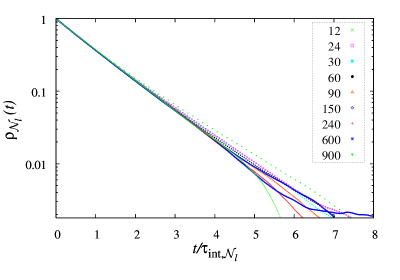
Figure 7: Autocorrelation function $\rho_{\mathcal{N}_{l}}(t)$ versus $t/\tau_{{\rm int},\mathcal{N}_{l}}$. It is clear that $\rho_{\mathcal{N}_{l}}(t)$ decays almost as a pure exponential, suggesting $z_{\rm exp}\approx z_{{\rm int},\mathcal{N}_{l}}$.

We fitted the $\tau_{{\rm int},\mathcal{N}_{l}}$ data to the ansatz

$$\tau_{{\rm int}}=a+bL^{z_{{\rm int}}+2X_{h}},$$ (3.10)

which produced the estimate

$$z_{{\rm int},\mathcal{N}_{l}}=0.515(8),$$

suggesting

$$z_{\exp}=0.515(8).$$

Assuming $z_{\exp}=z_{\text{int},\mathcal{N}_{l}}$, the long-time decay of the autocorrelation function for any observable $\mathcal{O}$ should behave like $\rho_{\mathcal{O}}(t)\sim\exp(-t/\tau_{\text{int},\mathcal{N}_{l}})$. However, it was observed in [17] that for the standard worm algorithm simulating the critical Ising model on the square and simple cubic lattices, some observables can have quite unusual short-time dynamics. Indeed it was found that $\mathcal{D}_{0}$ decorrelated in $O(1)$ hits and a detailed investigation of $\rho_{\mathcal{D}_{0}}(t)$ was presented. This phenomenon in which some observables decorrelate on time scales much less than $L^{z_{\exp}}$ has been dubbed critical speeding-up [36, 20, 17]. We have not performed a detailed investigation of the behavior of $\rho_{\mathcal{D}_{0}}(t)$ here, however we note that $\tau_{\text{int},\mathcal{D}_{0}}\approx 0.5$, independent of $L$, showing clearly that $\mathcal{D}_{0}$ certainly exhibits critical speeding-up under the dynamics of Algorithm 1. For $\mathcal{L}_{2}$ and $\mathcal{G}_{2}$ the short-time decay of $\rho(t)$ appears to be intermediate between that of $\mathcal{N}_{l}$ and $\mathcal{D}_{0}$. To illustrate, in Fig. 8 we plot $\rho_{\mathcal{L}_{2}}(t/\tau_{\text{int},\mathcal{N}_{l}})$.

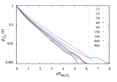
Figure 8: Autocorrelation function $\rho_{\mathcal{L}_{2}}(t)$ versus $t/\tau_{{\rm int},\mathcal{N}_{l}}$.

It appears that $\rho_{\mathcal{L}}(t)$ has a short-time decay on a time scale strictly less than $L^{z_{\exp}}$. Similar behavior is observed for $\rho_{\mathcal{G}_{2}}(t)$.

4 Discussion

We have formulated a worm algorithm that correctly simulates the FPL model on the honeycomb lattice when $n=1$. Furthermore, we have rigorously proved its validity by showing that the corresponding Markov chain is irreducible and has uniform stationary distribution. Using standard duality relations this algorithm can also be used to simulate the zero-temperature triangular-lattice antiferromagnetic Ising model.

We have tested this worm algorithm numerically and estimate $z_{\exp}=0.515(8)$, which suggests that it suffers from only mild critical slowing down. We observe that the dynamics of the algorithm exhibits the multi-time-scale behavior observed in [17]. It would be interesting to to examine the dynamic behavior of observables other than $\mathcal{N}_{l}$ in more detail, along the lines presented in [17], but this we leave to future work. We also obtained some interesting results regarding the static behavior of the FPL model, notably that the face-size moments appear to be governed by the magnetic dimension for percolation. This is consistent with the argument in [29] that the FPL model for general $n$ displays simultaneously the universal properties of a densely-packed loop model and those of a model with central charge $c=1$ and thermal dimension $X_{t}=1$.

Finally, we note that one could in principle simulate (1.3) with $n>1$ by incorporating appropriate connectivity checking into the Metropolis acceptance probabilities, or by combining an $n=1$ worm algorithm with a “Chayes-Machta coloring” as described in [37].

Appendix A Topological constraints on fully-packed subgraphs of the honeycomb lattice

The following lemmas describe some topological constraints on fully-packed spanning subgraphs of the honeycomb lattice with periodic boundary conditions. They are completely independent of any considerations regarding worm algorithms. We make essential use of Lemma A.1 in the proof of Proposition 2.2.

Lemma A.1.

If $(A,u,v)\in\mathcal{R}$ and $u\sim v$ then $d_{u}(A)=d_{v}(A)$.

Lemma A.2.

Let $(A,u,v)\in\mathcal{R}$, and let $H_{i}$, $U_{i}$, $D_{i}$ denote, respectively, the number of vacant horizontal edges, the number of occupied up-pointing vertical edges, and the number of occupied down-pointing vertical edges, in row $i$. If row $i$ contains no defects we have $H_{i}=U_{i}=D_{i}$.

Proof..

Fix a configuration $(A,u,v)\in\mathcal{R}$, and a row $i$ which contains no defects. Full-packing then implies that every vertex in this row has degree 2, so that for every vacant horizontal edge, one of its endpoints must be adjacent to an occupied up-pointing vertical edge and its other endpoint must be adjacent to an occupied down-pointing vertical edge, so $H_{i}\leq U_{i}$ and $H_{i}\leq D_{i}$. See Fig 9. Conversely, if $u$ is a vertex in row $i$ which is adjacent to an occupied down-pointing vertical edge then precisely one of its horizontal edges must be vacant, so $D_{i}\leq H_{i}$ and therefore $D_{i}=H_{i}$. Similarly, if $v$ is a vertex in row $i$ which is adjacent to an occupied up-pointing vertical edge then precisely one of its horizontal edges must be vacant, so $U_{i}\leq H_{i}$ and therefore $U_{i}=H_{i}$. ∎

Figure 9: If the horizontal edge $uv$ is vacant, and neither $u$ nor $v$ is a defect, the remaining edges incident to both $u$ and $v$ are forced to be occupied, in a fully packed configuration. Conversely, if the up-pointing vertical edge $vw$ is occupied, then precisely one of the horizontal edges incident to $v$ must be vacant (here $uv$), and the down-pointing vertical edge $ut$ must then be occupied. In the diagram, thick edges are occupied, thin edges are vacant, and dotted edges are unconstrained by the state of $uv$.

Proof of Lemma A.1.

Let us first note that there do indeed exist configurations with $d_{u}(A)=d_{v}(A)$ when $(A,u,v)\in\mathcal{R}$ and $u\sim v$. Indeed, if $(A,u,u)\in\mathcal{R}$ and $v\sim u$ then $(A\triangle uv,u,v)\in\mathcal{R}$; if $uv\in A$ then $d_{u}(A\triangle uv)=1=d_{v}(A\triangle uv)$, whereas if $uv\not\in A$ then $d_{u}(A\triangle uv)=3=d_{v}(A\triangle uv)$.

Suppose on the contrary that $(A,u,v)\in\mathcal{R}$ with $u\sim v$, but $d_{u}(A)\neq d_{v}(A)$. Since $u\neq v$ we must have $d_{u}(A),d_{v}(A)\in\{1,3\}$, so that either $d_{u}(A)=3$ and $d_{v}(A)=1$, or vice versa. Let us assume (without loss of generality) the former. There are two possibilities for the edge $uv$; either $uv$ is a horizontal edge, so that $u$ and $v$ lie in the same row, or $uv$ is a vertical edge, so that $u$ and $v$ lie in adjacent rows.

Figure 10: Neighborhood of the horizontal edge $uv$ with $d_{u}(A)=3$ and $d_{v}(A)=1$.

Suppose $uv$ is a horizontal edge lying in row $i$, denote $v$’s other horizontal edge by $vw$, and suppose that the vertical edge $uu^{\prime}$ is up-pointing, so that the vertical edge $vv^{\prime}$ must be down-pointing. See Fig. 10. The up-pointing vertical edges $uu^{\prime}$ and $ww^{\prime}$ are both occupied. Suppose there are $n$ other occupied up-pointing vertical edges incident to row $i$, so there are $n+2$ in total. Each of these other $n$ occupied up-pointing vertical edges is incident to a degree 2 vertex in row $i$. Let $a$ be such a vertex, then $a$ must have one of its horizontal edges vacant, call it $ab$. By assumption we have $a\neq u,w$, so that $b\neq v$, and so $d_{b}(A)=2$ and $b$ must have its vertical edge (which is down-pointing) occupied. Therefore, every one of the $n$ occupied up-pointing vertical edges other than $uu^{\prime}$ and $ww^{\prime}$ corresponds to an occupied down-pointing vertical edge. Conversely, if there is an occupied down-pointing vertical edge incident to some $b\neq v$ in row $i$ then $b$ must have one of its horizontal edges vacant, call it $ab$. Since $b\neq v$ and $ab$ is vacant we have $a\neq u,w$, so that $d_{a}(A)=2$. Therefore $a$ must have its vertical edge (which is up-pointing) occupied, and this edge is neither $uu^{\prime}$ nor $ww^{\prime}$. Therefore there are $n$ occupied down-pointing and $n+2$ occupied up-pointing vertical edges incident to row $i$. Now, since no other row contains a defect, Lemma A.2 tells us that all rows below row $i$ will have $n$ occupied up-pointing and down-pointing vertical edges, whereas all rows above row $i$ will have $n+2$ occupied up-pointing and down-pointing vertical edges. However, it is impossible for this to occur if we have periodic boundary conditions, and so we have a contradiction. Of course, if we assume instead that $u$ is down-pointing and $v$ up-pointing then an entirely similar argument leads to a similar contradiction. Therefore if $(A,u,v)\in\mathcal{R}$ and $uv$ is a horizontal edge we must have $d_{u}(A)=d_{v}(A)$.

The converse situation where $uv$ is a vertical edge can be treated in a similar manner. We omit the details. ∎

Appendix B Lemmas used in the proof of Proposition 2.3

Lemma B.1.

Let $(A,v,v)\in\mathcal{S}$ with $vv^{\prime}\not\in A$. Then whenever $d_{v}(A)=2$ we have

$$(A,v,v)\rightarrow(A\cup vv^{\prime},v^{\prime},v)\rightarrow(A,v^{\prime},v^{\prime}),$$

and whenever $d_{v}(A)=d_{v^{\prime}}(A)=2$ we have

$$(A,v,v)\rightarrow(A\setminus vv^{\prime\prime},v^{\prime\prime},v)\rightarrow(A,v^{\prime\prime},v^{\prime\prime}),$$

for both $v^{\prime\prime}\sim v$ with $v^{\prime\prime}\neq v^{\prime}$.

Lemma B.2.

Let $H\in F_{\mathbb{H}}$ denote the fully-packed configuration in which every horizontal edge is occupied and every vertical edge is vacant. Suppose $(A,u,u)\in\mathcal{S}$ with $d_{u}(A)=2$ and $A\neq H$. Then there always exists a vacant horizontal edge $vv^{\prime}$ for which $(A,u,u)\rightarrow(A,v,v)$.

Lemma B.3.

If $(A,v,v)\in\mathcal{R}$ then $(A,v,v)\leftrightarrow(A,u,u)$ for any pair of vertices $u$ and $v$.

Lemma B.4.

If $(A,v,v)\in\mathcal{R}$ and $u\sim v$ then

$$(A,v,v)\leftrightarrow(A\triangle uv,u,v).$$

Lemma B.5.

Let $(A,u,v)\in\mathcal{R}$ with $d_{u}(A)=1$ and suppose $uu^{\prime}\not\in A$. Then

$$(A,u,v)\leftrightarrow(A\cup uu^{\prime},u^{\prime},v)$$

Lemma B.6.

If $(A,u,v)\in\mathcal{R}$ with $d_{u}(A)=3$ then for each $u^{\prime}\sim u$

$$(A,u,v)\leftrightarrow(A\setminus uu^{\prime},u^{\prime},v).$$

Proof of Lemma B.1.

For any $(A,v,v)\in\mathcal{S}$ with $vv^{\prime}\not\in A$ we have

$$P_{\infty}^{\prime}[(A,v,v)\rightarrow(A\cup vv^{\prime},v^{\prime},v)]=1/6.$$

Furthermore, if $d_{v}(A)=2$ then $d_{v}(A\cup vv^{\prime})=3$ so

$$P_{\infty}^{\prime}[(A\cup vv^{\prime},v^{\prime},v)\rightarrow(A,v^{\prime},v^{\prime})]=1/6$$

and we have

$$(A,v,v)\rightarrow(A\cup vv^{\prime},v^{\prime},v)\rightarrow(A,v^{\prime},v^{\prime}).$$

If in fact $d_{v}(A)=2=d_{v^{\prime}}(A)$ then for both $v^{\prime\prime}\sim v$ with $v^{\prime\prime}\neq v^{\prime}$ we have

$$P_{\infty}^{\prime}[(A,v,v)\rightarrow(A\cup vv^{\prime},v,v^{\prime})] =1/6$$

$$P_{\infty}^{\prime}[(A\cup vv^{\prime},v,v^{\prime})\rightarrow(A\cup vv^{\prime}\setminus vv^{\prime\prime},v^{\prime\prime},v^{\prime})] =1/6$$

$$P_{\infty}^{\prime}[(A\cup vv^{\prime}\setminus vv^{\prime\prime},v^{\prime\prime},v^{\prime})\rightarrow(A\setminus vv^{\prime\prime},v^{\prime\prime},v)] =1/6$$

$$P_{\infty}^{\prime}[(A\setminus vv^{\prime\prime},v^{\prime\prime},v)\rightarrow(A,v^{\prime\prime},v^{\prime\prime})] =1/4$$

so that

$$(A,v,v)\rightarrow(A\setminus vv^{\prime\prime},v^{\prime\prime},v)\rightarrow(A,v^{\prime\prime},v^{\prime\prime}).$$

∎

Proof of Lemma B.2.

Denote by $uu^{\prime}\not\in A$ the unique vacant edge incident to $u$. There are two possibilities: either $d_{u^{\prime}}(A)=0$ or $d_{u^{\prime}}(A)=2$. If $d_{u^{\prime}}(A)=0$ then $u^{\prime}$ has both its incident horizontal edges vacant, and since Lemma B.1 implies $(A,u,u)\rightarrow(A,u^{\prime},u^{\prime})$ there is nothing more to show. If on the other hand $d_{u^{\prime}}(A)=2$ then Lemma B.1 implies $(A,u,u)\rightarrow(A,v,v)$ for every $v\sim u$. If any of the $(A,v,v)$ have a vacant horizontal edge incident to $v$ we are done. Otherwise we re-apply Lemma B.1 to $(A,v,v)$ for every $v\sim u$. In this way we must eventually arrive at some $(A,w,w)$ for which there is a vacant horizontal edge incident to $w$. Transitivity implies $(A,u,u)\rightarrow(A,w,w)$ and the stated result follows. ∎

Proof of Lemma B.3.

If $(A,v,v)\in\mathcal{R}$ then in fact $(A,u,u)\in\mathcal{R}$ for any $u$. Since every vertex has degree 2 we can apply Lemma B.1 to $(A,v,v)$ to see that $(A,v,v)\rightarrow(A,v^{\prime},v^{\prime})$ for any $v^{\prime}\sim v$, but we can equally apply it to $(A,v^{\prime},v^{\prime}$) to see that $(A,v^{\prime},v^{\prime})\to(A,v,v)$. So for any pair of neighboring vertices $v\sim v^{\prime}$ we have $(A,v,v)\leftrightarrow(A,v^{\prime},v^{\prime})$. Since the lattice is connected and every vertex has degree 2 this immediately extends, via transitivity of $\leftrightarrow$, to $(A,v,v)\leftrightarrow(A,u,u)$ for any arbitrary pair or vertices $u,v$. ∎

Proof of Lemma B.4.

Let $(A,v,v)\in\mathcal{R}$ and $u\sim v$. Lemma B.1 immediately implies

$$(A,v,v)\rightarrow(A\triangle uv,u,v)$$

and combining Lemma B.1 with Lemma B.3 we further obtain

$$(A\triangle uv,u,v)\rightarrow(A,u,u)\rightarrow(A,v,v).$$

Therefore $(A,v,v)\leftrightarrow(A\triangle uv,u,v)$. ∎

Proof of Lemma B.5.

Suppose that $u^{\prime}\neq v$. Then

$$P_{\infty}^{\prime}[(A,u,v)\to(A\cup uu^{\prime},u^{\prime},v)]=\frac{1}{4},$$

and since $u^{\prime}\neq v$ implies $d_{u^{\prime}}(A)=2$ we have $d_{u^{\prime}}(A\cup uu^{\prime})=3$, so that

$$P_{\infty}^{\prime}[(A\cup uu^{\prime},u^{\prime},v)\to(A,u,v)]=\frac{1}{6}.$$ (B.1)

Therefore $(A,u,v)\leftrightarrow(A\cup uu^{\prime},u^{\prime},v)$ when $u^{\prime}\neq v$.

Conversely, suppose $u^{\prime}=v$. Then Lemma B.4 implies that $(A\cup uv,v,v)\leftrightarrow(A,u,v)$. ∎

Proof of Lemma B.6.

Suppose that $u^{\prime}\neq v$. Since $d_{u}(A)=3$

$$P_{\infty}^{\prime}[(A,u,v)\to(A\setminus uu^{\prime},u^{\prime},v)]=\frac{1}{6}.$$

Furthermore, since $u^{\prime}\neq v$ we have $d_{u^{\prime}}(A)=2$ and hence $d_{u^{\prime}}(A\setminus uu^{\prime})=1$, so

$$P_{\infty}^{\prime}[(A\setminus uu^{\prime},u^{\prime},v)\to(A,u,v)]=\frac{1}{4}.$$

Therefore $(A,u,v)\leftrightarrow(A\setminus uu^{\prime},u^{\prime},v)$ when $u^{\prime}\neq v$.

Conversely, suppose $u^{\prime}=v$. Then Lemma B.4 implies that $(A\setminus uv,v,v)\leftrightarrow(A,u,v)$. ∎

References

- [1] G. H. Wannier, Phys. Rev. 79 (1950) 357.
- [2] J. Stephenson, J. Math. Phys. 5 (1964) 1009.
- [3] H. J. H. B. Nienhuis, H. W. J. Blöte, J. Phys. A 17 (1984) 3559.
- [4] H. W. J. Blöte, M. P. Nightingale, Phys. Rev. B 47 (1993) 15046.
- [5] S. L. A. de Quieroz, E. Domany, Phys. Rev. E 52 (1994) 4768.
- [6] X. F. Qian, H. W. J. Blöte, Phys. Rev. E 70 (2004) 036112.
- [7] X. F. Qian, M. Wegewijs, H. W. J. Blöte, Phys. Rev. E 69 (2004) 036127.
- [8] E. Rastelli, S. Regina, A. Tassi, Phys. Rev. B 71 (2005) 174406.
- [9] K. Xia, X.-Y. Yao, J.-M. Liu, Frontier of Phys. in China 2 (2007) 191.
- [10] G. M. Zhang, C. Z. Yang, Phys. Rev. B 50 (1994) 12546–12549.
- [11] P. D. Coddington, L. Han, Phys. Rev. B 50 (1994) 3058.
- [12] D. Kandel, R. Ben-Av, E. Domany, Phys. Rev. B 45 (1992) 4700.
- [13] A. Dhar, P.Chaudhuri, C. Dasgupta, Phys. Rev. B 61 (2000) 6227.
- [14] R. H. Swendsen, J.-S. Wang, Phys. Rev. Lett. 58 (1987) 86–88.
- [15] N. Prokof’ev, B. Svistunov, Phys. Rev. Lett. 87 (2001) 160601.
- [16] M. Jerrum, A. Sinclair, SIAM J. Comput. 22 (1993) 1087.
- [17] Y. Deng, T. M. Garoni, A. D. Sokal, Phys. Rev. Lett. 99 (2007) 110601.
- [18] U. Wolff, Simulating the All-Order Strong Coupling Expansion I: Ising Model Demo, arXiv:0808.3934v1 [hep-lat].
- [19] M. Sweeny, Phys. Rev. B 27 (1983) 4445–4455.
- [20] Y. Deng, T. M. Garoni, A. D. Sokal, Phys. Rev. Lett. 98 (2007) 230602.
- [21] L. Chayes, J. Machta, Physica A. 254 (1998) 477–516.
- [22] B. Nienhuis, Phys. Rev. Lett. 49 (1982) 1062.
- [23] B. Nienhuis, J. Stat. Phys. 34 (1984) 731.
- [24] P. Di Francesco, P. Mathieu, D. Sénéchal, Conformal Field Theory, Springer-Verlag, New York, 1997.
- [25] O. Schramm, Israel J. Math. 118 (2000) 221.
- [26] S. Rohde, O. Schramm, Ann. Math. 161 (2005) 883.
- [27] G. Lawler, Conformally Invariant Processes in the Plane, American Mathematical Society, Providence, 2005.
- [28] H. Blöte, B. Nienhuis, Physica A. 160 (1989) 121.
- [29] H. W. J. Blöte, B. Nienhuis, Phys. Rev. Lett. 72 (1994) 1372.
- [30] A. D. Sokal, Monte Carlo methods in statistical mechanics: Foundations and new algorithms, in: P. C. C. DeWitt-Morette, A. Folacci (Eds.), Functional Integration: Basics and Applications, Plenum, New York, 1997, pp. 131–192.
- [31] J. G. Kemeny, J. L. Snell, Finite Markov Chains, Springer-Verlag, New York, 1976.
- [32] J.-S. Wang, Phys. Rev. E 72 (2005) 036706.
- [33] M. Iosifescu, Finite Markov Processes and Their Applications, John Wiley & Sons, Bucharest, 1980.
- [34] G. Grimmett, D. Stirzaker, Probability and Random Processes, 3rd Edition, Oxford University Press, New York, 2006.
- [35] P. C. Hohenberg, B. I. Halperin, Rev. Mod. Phys. 49 (1977) 435.
- [36] Y. Deng, T. M. Garoni, A. D. Sokal, Phys. Rev. Lett. 98 (2007) 030602.
- [37] Y. Deng, T. M. Garoni, W. Guo, H. W. J. Blöte, A. D. Sokal, Phys. Rev. Lett. 98 (2007) 120601.