Structure of the fermion propagator in QED₃

Abstract:

The Minkowski structure of the Fermion propagator in $QED_{2+1}$ is evaluated using a dispersion like method. Including a massive fermion loop to the photon spectral function, there is no infrared divergences in the $d=-1$ gauge. Screening effects suppress the chiral order parmeter for small numbers of fermion flavour $N$. We evaluate $\langle\overline{\psi}\psi\rangle$ as a function of the coupling constant $c$ and $N$. There exists a region where chiral symmetry is dynamically broken.

1 Introduction

It has been known that dynamical mass generation and chiral symmetry breaking occur in QED₃ by solving Dyson-Schwinger (D-S) equation or by computer simulation on a lattice [1, 2, 3, 4]. Including massless fermion loop to the photon vacuum polarization, critical behaviour has been studied which was first pointed out by Appelquist et.al [2]. The results have not been conclusive for the existence of critical numbers of flavours. In this work we adopt the alternative approach to the phase structure of QED₃ by a dispersion like method. We evaluate the spectral function for fermion. Assuming physical mass, we examine the infrared behaviour with a soft photon cloud. As a result, we obtain a gauge invariant anomalous dimension and a mass shift in the lowest spectral function in the quenched approximation. Full spectral function is given by exponentiation of the lowest one. If we include the massive fermion loop to the spectral function of photon, there is no infrared divergences in the $d=-1$ gauge. When the anomalous dimension equals to one, the propagator behaves as $1/p^{4}$ at high energy and dynamical chiral symmetry breaking takes place. The screening effects are large to reduce renormalization constant $Z_{3}^{-1}$ for smal numbers of flavour $N$. We study chiral order parameter $\left\langle\overline{\psi}\psi\right\rangle$ as a function of $N$ and the coupling constant $c.$ We show that there is a region in which chiral symmetry is dynamically broken.

2 Dispersion approach

The spectral function of a fermion [5, 6] is defined by

$$S_{F}(x) = S_{F}^{0}(x)\exp(F(x))$$ (1)

$$S_{F}^{0}(x) = -(i\gamma\cdot\partial+m)\frac{\exp(-m\sqrt{x^{2}})}{4\pi\sqrt{x^{2}}},$$ (2)

where $F$ is an $O(e^{2})$ matrix element $|T_{1}|^{2}$ for the process electron($p)\rightarrow$electron($r)+$photon($k)$ given by

$$F=-e^{2}\int\frac{d^{3}k}{(2\pi)^{2}}\exp(ikx)\theta(k_{0})\delta(k^{2}-\mu^{2})[\frac{m^{2}}{(r\cdot k)^{2}}+\frac{1}{r\cdot k}+\frac{(d-1)}{k^{2}}].$$ (3)

It is well known that the function $F$ has linear and logarithmic infrared divergences with respect to $\mu$ where $\mu$ is a bare photon mass. Here we notice the following

1. $\exp(F)$ includes all infrared divergences.

2. The quenched propagator has linear and logarithmic infrared divergences.

Linear divergence is absent in a special gauge. To remove logarithmic divergences we include a massive fermion loop. The photon propagator is then written in spectral form

$$D_{F}(p)=-\int_{0}^{\infty}\frac{\rho_{\gamma}(\mu^{2})d\mu^{2}}{p^{2}-\mu^{2}+i\epsilon}.$$ (4)

3 Screening effects

We show here the effects of massive fermion loop on the photon renormalization constant and spectral function. The vacuum polarization of the four component massive fermion is [6]

$$\Pi(k) = -\frac{e^{2}}{8\pi}[(\sqrt{-k^{2}}+\frac{4m^{2}}{\sqrt{-k^{2}}})\ln(\frac{2m+\sqrt{-k^{2}}}{2m-\sqrt{-k^{2}}})-4m],$$ (5)

$$= -\frac{e^{2}}{8}i\sqrt{-k^{2}}(-k^{2}>0,m=0),$$

$$= \frac{e^{2}}{6\pi m}k^{2}+O(k^{4})(-k^{2}/m\ll 1).$$

In the massless photon approximation, the effects of screening is the largest. We get the photon spectral function by the imaginary part of the dressed photon propagator

$$\rho_{\gamma}(k^{2})=\frac{\mbox{Im}D_{F}(k)}{\pi}=\frac{1}{\pi}\mbox{Im}\frac{1}{(-k^{2}-\Pi(k))}.$$ (6)

The renormalization constant of the photon field is defined by

$$Z_{3}^{-1}=\int_{0}^{\infty}\rho_{\gamma}(s)ds.$$ (7)

There is a masless pole $\delta(s)$ for $m\neq 0.$ But it does not contribute to the fermion propagator. In that case, the fermion propagator vanishes in the limit $\mu\rightarrow 0.$ In numerical analysis, we set $m=c/N\pi,c=e^{2}N/8$ which are expected in the $1/N$ approximation.

3.1 Quenched case

The function $F$ is evaluated in the covariant gauge [7]

$$F =\frac{e^{2}}{8\pi}[\frac{\exp(-\mu|x|)-\mu|x|E_{1}(\mu|x|)}{\mu}-\frac{E_{1}(\mu|x|)}{m}$$ (8)

$$+\frac{(d-1)\exp(-\mu\left|x\right|))}{2\mu}],|x|=\sqrt{x^{2}}.$$

For short and long distance, we have the approximate form of the function $F$

$$F_{S}\sim A-\mu|x|+(D+C|x|)\ln(\mu\left|x\right|))-\frac{(d+1-2\gamma)e^{2}|x|}{16\pi},(\mu|x|\ll 1).$$ (9)

$$F_{L}\sim 0,(1\ll\mu|x|).$$ (10)

From the above formulae, we have the approximate form of the spectral function $\exp(F)$

$$\exp(F)=(\begin{array}[c]{c}A(\mu|x|)^{D+C|x|}(\mu|x|\leq 1)\\ 1(1\leq\mu|x|)\end{array}),$$ (11)

where $m$ is the physical mass and

$$A=\exp(\frac{e^{2}(1+d)}{16\pi\mu}+\frac{e^{2}\gamma}{8\pi m}),C=\frac{e^{2}}{8\pi},D=\frac{e^{2}}{8\pi m},$$ (12)

where $\gamma$ is the Euler’s constant. From the above short distance behaviour of $F$, we obtain the mass shift and the position dependent mass as

$$\triangle m=\frac{e^{2}(1+d-2\gamma)}{16\pi}+\frac{e^{2}\mu}{8\pi m},m(x)=m-C\ln(\mu\left|x\right|),$$ (13)

We see here that $D$ acts to change the power of $|x|$. For $D=1,S_{F}(0)$ is finite and we have $\left\langle\overline{\psi}\psi\right\rangle\neq 0.$ Thus if we require $D=1,$ we obtain $m=e^{2}/8\pi.$

3.2 Unquenched case

In the unquenched case, we replace the quenched spectral function for the photon by the dressed one

$$\exp(F(x))\rightarrow\int_{0}^{\infty}\rho_{\gamma}(s)\exp(F(x,s)ds.$$ (14)

From now on, we fix the gauge $d=-1$ to avoid linear infrared divergences. There exists a massless photon pole contribution to $\rho_{\gamma}(s).$ However, if we take a limit $\mu\rightarrow 0$, the fermion propagator vanishes, which can be seen from eq(3.7). In Fig.1,2 we see the $N$ dependence of screening effects on the renormalization constant $Z_{3}^{-1}$ and the function $\exp(\widetilde{F}(x))$ respectively. From these figure we see that the screening effects are large for small $N.$

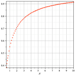
Figure 1: $Z_{3}^{-1}-1$ for $m\neq 0,N=1/2$ $..10.$

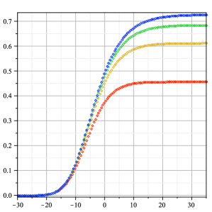
Figure 2: $\exp(\widetilde{F}(x))$ for $N=1,2,3$ with $x=\exp(\pi/2\sinh(l/5)).$

4 Minkowski space

Here we change the variable $x^{2}\rightarrow iT,s=p^{2}/m^{2}$ [5, 8] and define the spectral function of fermion $\rho(s)$ as

$$\exp(\widetilde{F}(iT))=\int_{0}^{\infty}d\sigma\rho^{F}(\sigma)\exp(F(iT,\sqrt{\sigma})),$$ (15)

$$\rho(s)=\frac{1}{2\pi}\int_{-\infty}^{\infty}\exp(-i(s-1)T)\Im(\exp(\widetilde{F}(iT))dT.$$ (16)

In Fig.3, the spectral function $\rho(s)$, in unit of $e^{2}$, has sharp peaks for both side of $s=1$ for $N=2,3$. For $N=1$ these peaks are wide. We see that the real part of the propagator has no pole like singularity in Fig.4, where $s=\ln(2/(1-\mbox{erf}(l/5))$.

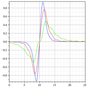
Figure 3: $\rho(s)$ for $N=1(bottom),2,3(top)$ in unit of $e^{2}.$

Figure 4: $\Re(S_{S}(s)4\pi$ for $N=1(bottom),2,3(top)$ in unit of $e^{2}.$

For strong coupling, the spectral function has no peak which corresponds to the double pole structure. This may be due to the large mass changing effects which appeared as $c|x|\ln(\mu|x|)-c|x|.$

5 Renormalization constant and order parameter

In the beginning, we assume the asymptotic field :$\psi(x)_{t\rightarrow+\infty,-\infty}\rightarrow\sqrt{Z_{2}}\psi(x)_{out,in}.$ The integral representation of the propagator is written

$$S_{F}^{{}^{\prime}}(p)=\int_{m^{2}}^{\infty}\frac{(\gamma\cdot p+m)\rho(s)ds}{p^{2}-s+i\epsilon}.$$ (17)

However in our approximation we have

$$Z_{2}^{-1}=\int_{0}^{\infty}\rho(s)ds=\int_{-\infty}^{\infty}dt\delta_{+}(t)\mbox{Im}(\exp(F(it)))=0,$$ (18)

$$m_{0}Z_{2}^{-1}=0,$$ (19)

for the case of positive anomalous dimention. Our approximation contains the analytic solution for the linear D-S equation in the quenched Landau gauge [9].

Figure 5: $-\left\langle\overline{\psi}\psi\right\rangle$ in unit of $c=1.$

$$S_{S}(p)=\frac{m^{3}}{(p^{2}+m^{2})^{2}},\mbox{Im}S_{S}(p)=-m^{3}\delta^{\prime}(p^{2}-m^{2}).$$ (20)

This behaviour is seen for weak coupling in our approximation. For $D\mathbf{=}1,$ $m=c/N\pi$ we have $\left\langle\overline{\psi}\psi\right\rangle=-4\lim_{x\rightarrow 0}m\overline{\rho}(x),\left\langle\overline{\psi}\psi\right\rangle\approx-(6.7-2.2)10^{-3}e^{2}$ for $N=1-3.$ In the case of a massless fermion loop, the results are $(2.8-2.2)10^{-3}e^{2}$ for $N=1-3$ in the same way. These values are consistent with those obtained $(3.33,1.2)10^{-3}e^{2}$ for $N=0,1$ in D-S eq with massless fermion loop and kinds of vertex ansatz [3]. Finally we show the order parameter $\left\langle\overline{\psi}\psi\right\rangle$ as a function of $N$ and the coupling constant $c$. Here we notice that $\left\langle\overline{\psi}\psi\right\rangle$ equals to zero for $N\leq 2/\pi$ for $c=e^{2}N/8=1$ in Fig.5. In this mass region, $m=c/N$  is large enough and vacuum polarization is suppressed in such a way that $c/2m=N\pi/2\ll 1$. In this case, the photon propagator is the quenched one and $\left\langle\overline{\psi}\psi\right\rangle$ vanishes. If we fix $N$ and vary the coupling constant $c,$ large $c$ corresponds to the quenched case and there exists a critical coupling $c_{r}=\pi N/2$ below which $\left\langle\overline{\psi}\psi\right\rangle\neq 0.$ This phenomenon is the same with finite temperature phase transition in superconductivity. In the case of a massless fermion loop, there is only a broken phase from the above reasons.

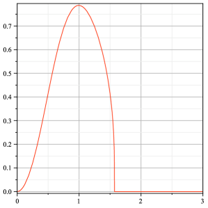
Figure 6: $-\left\langle\overline{\psi}\psi\right\rangle(c)$ for $N=1.$

6 Summary

In this work, we examined whether the dispersion like method works or not to determine the non perturbative fermion propagator in QED3. If we assume physical mass, we have a mass shift, its log correction and anomalous dimension in the lowest order spectral function. There is a gauge $d=-1$ in which linear divergences vanish. Including vacuum polarization, the logarithmic infrared divergence disappeared. As a results, there is no infrared divergences and no poles. There exists a critical coupling constant such as critical temperature in superconductivity. We have seen that the dispersion like method works well in QED3. In the future, we will analyse finite temperature case, QCD(2+1), and its application to high-T_c superconductivity.