On the evolution of mean motion resonances through stochastic forcing: Fast and slow libration modes and the origin of HD128311

Abstract

Aims. We clarify the response of extrasolar planetary systems in a 2:1 mean motion commensurability with masses ranging from the super Jovian range to the terrestrial range to stochastic forcing that could result from protoplanetary disk turbulence. The behaviour of the different libration modes for a wide range of system parameters and stochastic forcing magnitudes is investigated. The growth of libration amplitudes is parameterized as a function of the relevant physical parameters. The results are applied to provide an explanation of the configuration of the HD128311 system.

Methods. We first develop an analytic model from first principles without making the assumption that both eccentricities are small. We also perform numerical N-body simulations with additional stochastic forcing terms to represent the effects of putative disk turbulence.

Results. We isolate two distinct libration modes for the resonant angles. These react to stochastic forcing in a different way and become coupled when the libration amplitudes are large. Systems are quickly destabilized by large magnitudes of stochastic forcing but some stability is imparted should systems undergo a net orbital migration. The slow mode, which mostly corresponds to motion of the angle between the apsidal lines of the two planets, is converted to circulation more readily than the fast mode which is associated with oscillations of the semi-major axes. This mode is also vulnerable to the attainment of small eccentricities which causes oscillations between periods of libration and circulation.

Conclusions. Stochastic forcing due to disk turbulence may have played a role in shaping the configurations of observed systems in mean motion resonance. It naturally provides a mechanism for accounting for the HD128311 system for which the fast mode librates and the slow mode is apparently near the borderline between libration and circulation.

1 Introduction

Of the recently discovered 335 extrasolar planets, at least 75 are in multiple planet systems (Schneider 2009). About 10% of these are in or very close to a resonant configuration where two planets show a mean motion commensurability, with four systems in or near a 2:1 resonance (Udry et al. 2007; Reipurth et al. 2007).

Resonant configurations can be established by dissipative forces acting on the planets which lead to convergent migration (see for example Lee & Peale 2001; Snellgrove et al. 2001). An anomalous effective kinematic viscosity $\nu$ of order $\sim 10^{-5},$ but with considerable uncertainty, has been inferred from observations of accretion rates onto the central protostars. The magneto rotational instability (MRI) is thought to be responsible for this anomalous value of $\nu$ which is often characterized using the Shakura & Sunyaev (1973) $\alpha=\nu/(c_{s}\Omega)$ parameter, with $c_{s}$ being the local sound speed and $2\pi/\Omega$ being the orbital period. For the most likely situation of small or zero net magnetic flux, recent MHD simulations have indicated $\alpha\approx 10^{-2}-10^{-3}$. Even assuming adequate ionization, this value is uncertain when realistic values of the actual transport coefficients are employed because of numerical resolution issues (see Fromang & Papaloizou 2007; Fromang et al. 2007). Which parts of protoplanetary disks are adequately ionized, or consitute a dead zone, is also an issue (eg. Gammie 1996). Because the level of MRI turbulence and associated density fluctuations are very uncertain, we consider stochastic force amplitudes ranging over several orders of magnitude.

The influence of stochastic forces resulting from the gravitational field produced by the density fluctuations associated with MRI turbulence on migrating planets was explored first by Nelson & Papaloizou (2004). They considered MRI simulations directly with the result that the simulation ran only for a relatively small number of orbits. To consider much longer evolution times, as done here, a simpler parameterized model of the forcing is needed.

Recent studies by Adams et al. (2008) and Lecoanet et al. (2008) have been made in order to estimate the lifetimes of the mean motion resonances in the GJ876 system when it is perturbed by a sequence of stochastic kicks. They found that resonances were disrupted within expected disk lifetimes for sufficiently large forcing. They assume a fixed orbit for the outer planet and gave an interesting discussion of the interactions of the two planets based on a pendulum equation with an additional ad hoc stochastic forcing term. The aim of the work presented in this paper is to provide a more complete study of the full set of celestial mechanics equations and to describe the interplay between apsidal corotation and mean motion resonance as well as to consider a wide range of planet masses and stochastic force amplitudes. In addition, we derive a prescription for incorporating continuous stochastic forcing terms that allows for a general autocorrelation function with associated correlation time. Their magnitudes are related to properties of the protoplanetary disk and physical scaling laws are found. This is of particular importance as the factors that control the strength of the stochastic forcing are not well constrained. We also use our formalism to estimate the stochastic diffusion rates of the orbital elements from first principles.

We further remark that Adams et al. (2008) gave a discussion of the diffusion of resonant angles that do not satisfy the d’Alambert condition (see eg. Hamilton 1994) which is equivalent to the requirement of rotational invariance. Thus their appearrance cannot be straightforwardly connected to the basic equations or angles discussed in this paper unless one assumes that the variation of the longtitude of pericentre of one or both of the interacting planets can be neglected. However, the system lifetimes derived from their numerical work is broadly consistent with ours for the parameter regime they considered.

We find that stochastic forcing readily produces systems in mean motion resonance with broken apsidal corotation. An additional aim of this paper is to use this feature to construct scenarios involving convergent migration and stochastic forcing to account for the HD128311 system.

The plan of the paper is as follows. In section 2 we present the basic equations governing two interacting planets subject to external stochastic forces. We specialize to the case where the planets are either in or near a mean motion commensurability and so retain only the two angle variables that vary on a time scale much longer than the orbital one. Considering the case where these angles undergo small amplitude librations, we identify fast and slow libration modes, the former being associated with variations in the semi-major axes and the latter with the angle between the apsidal lines of the two planets. We go on to consider the effects of stochastic forcing arising from some external process such as disk turbulence in section 2.3 deriving the diffusion rates for the orbital elements of a single planet and the growth rate of the libration amplitudes in the two planet case.

In section 3 we discuss the origin and numerical implementation of the stochastic forcing and their operation in the single planet case. In section 4 we go on to consider the stochastic forcing in the two planet case. We consider the conversion of the fast and slow modes from libration to circulation for model systems of varying total mass ratio and initial eccentricities including GJ876. The attainment of small eccentricities and coupling to the fast mode results in conversion of the slow mode to circulation before the fast mode. Investigations are carried out for stochastic diffusion rates, proportional to the mean square stochastic force amplitude ranging over several orders of magnitude. The life time of the resonant angles is found to be inversely proportional to the diffusion rate except in the case of systems with low total mass in the earth mass range.

In section 5 we exploit the tendency of the slow mode, related to the angle between the apsidal lines, to be driven to circulate while the fast mode still librates in stochastically forced systems, to make a model for the formation of the HD128311 system which may be in such a state and was not readily understood in terms of convergent migration models for producing the commensurability. We combine the effects of such migration and stochastic forcing, showing that during the migration phase, while the librations tend to be stabilized, the slow mode is readily converted to circulation while the fast mode continues to librate. Good agreement is obtained with the somewhat uncertain observed orbital configuration. Finally in section 6 we summarize and discuss our results.

2 Basic Equations

We begin by writing down the equations of motion for a single planet moving in a fixed plane under a general Hamiltonian $H$ in the form (see e.g. Snellgrove et al. 2001; Papaloizou 2003)

$$\dot{E} = -n\frac{\partial H}{\partial\lambda}$$ (1)

$$\dot{G} = -\left(\frac{\partial H}{\partial\lambda}+\frac{\partial H}{\partial\varpi}\right)$$ (2)

$$\dot{\lambda} = \frac{\partial H}{\partial L}+n\frac{\partial H}{\partial E}$$ (3)

$$\dot{\varpi} = \frac{\partial H}{\partial L}.$$ (4)

Here the angular momentum of the planet is $G$ and the energy is $E.$ For orbital motion around a central point mass $M$ we have

$$G = m\sqrt{\mathcal{G}Ma(1-e^{2})}\hskip 14.22636pt{\rm and}$$ (5)

$$E = -{{\mathcal{G}Mm}\over{2a}},$$ (6)

where $\mathcal{G}$ is the gravitational constant, $a$ the semi-major axis and $e$ the eccentricity. The mean longtitude is $\lambda=n(t-t_{0})+\varpi,$ where $n$ the mean motion, with $t_{0}$ being the time of periastron passage and $\varpi$ being the longitude of periastron.

2.1 Additional Forcing of a Single Planet

In order to study the phenomena such as stochastic forcing we need to consider the effects of an additional external force per unit mass ${\bf F}$ which may not be described using a Hamiltonian formalism. However, as may be seen by considering general coordinate transformations starting from a Cartesian representation, the equations of motion are linear in the components of ${\bf F}$. Because of this we may determine them by considering forces of the form ${\bf F}=(F_{x},F_{y})$ for which the Cartesian components are constant. Having done this we may then suppose that these vary with coordinates and time in an arbitrary manner. Following this procedure we note that when ${\bf F},$ as in the above form is constant, we may derive the equations of motion by replacing the original Hamiltonian with a new Hamiltonian defined through

$$H \rightarrow H-m\left(F_{x}\;x+F_{y}\;y\right)=H-m\left(\mathbf{r}\cdot\mathbf{F}\right).$$ (7)

The additional terms proportional to the components of ${\bf F}$ correspond to the Gaussian form of the equations of motion (Brouwer & Clemence 1961).

The various derivatives involving $\mathbf{r}$ can be calculated by elementary means and expressed in terms of $E,G,\lambda$ and $\varpi.$ One thus finds additional contributions to the equations of motion (1) - (4), indicated with a subscript $F,$ in the form

$$\dot{G}_{F} = m\left(\frac{\partial}{\partial\lambda}+\frac{\partial}{\partial\varpi}\right)\;\left(\mathbf{r\cdot F}\right)=m\;\mathbf{\left(r\times F\right)\cdot\hat{e}}_{z}$$ (8)

$$\dot{E}_{F} = mn\frac{\partial}{\partial\lambda}\left(\mathbf{r\cdot F}\right)=m\;(\mathbf{v\cdot F})$$ (9)

$$\dot{\varpi}_{F} = -m\frac{\partial}{\partial L}\left(\mathbf{r\cdot F}\right)\ \ \ {\rm or\ \ equivalently}$$ (10)

$$\dot{\varpi}_{F} = \frac{\sqrt{(1-e^{2})}}{na\,e}\left[F_{\theta}\left(1+\frac{1}{{1-e^{2}}}\frac{r}{a}\right)\sin f-F_{r}\cos f\right]$$ (11)

$$\dot{\lambda}_{F} = -m\left(\frac{\partial}{\partial L}+n\frac{\partial}{\partial E}\right)\left(\mathbf{r\cdot F}\right)$$ (12)

$$= \left(1-\sqrt{1-e^{2}}\right)\dot{\varpi}_{F}+\frac{2an}{\mathcal{G}M}\;(\mathbf{r\cdot F}),$$ (13)

where the true anomaly $f$ is defined as the difference between the true longitude and the longitude of periastron, $f=\theta-\varpi.$ Note that from (9) we obtain

$$\dot{a}_{F}\ \ =\ \ -{2a\dot{n}\over 3n} = \frac{2({F_{r}}e\sin f+{F_{\theta}}(1+e\cos f))}{n\sqrt{1-e^{2}}}.$$ (14)

and from (8) together with (9) we obtain

$$\dot{e}_{F} = \frac{G(2E\dot{G}+G\dot{E})}{\mathcal{G}^{2}m^{3}M^{2}e}.$$ (15)

In the limit $e\ll 1$ this becomes (ignoring terms $O(e)$ and smaller)

$$\dot{e}_{F} = {F_{r}}\frac{1}{an}\sin f+{F_{\theta}}\frac{1}{an}2\cos f.$$ (16)

Furthermore in this limit we may replace $f$ by $f=\lambda-\varpi=n(t-t_{0}).$

We remark that the above formalism results in equation (11) which gives an expression for $\dot{\varpi}_{F}$ that indicates that this quantity diverges for small $e$ as ${1/e}.$ We comment that, as is well known, this aspect results from the choice of coordinates used and is not associated with any actual singularity or instability in the system. This is readily seen if one uses $h=e\sin\varpi,$ and $k=e\cos\varpi$ as dynamical variables rather than $e$ and $\varpi.$ The former set behave like Cartesian coordinates, while the latter set are the corresponding cylindrical polar coordinates. When the former set are used, potentially divergent terms $\propto 1/e$ do not appear. This can be seen from (11) and (16) which give in the small $e$ limit

$$\dot{h}_{F} = -{F_{r}}\frac{1}{an}\sin\lambda+{F_{\theta}}\frac{1}{an}2\cos\lambda$$ (17)

$$\dot{k}_{F} = {F_{r}}\frac{1}{an}\sin\lambda+{F_{\theta}}\frac{1}{an}2\cos\lambda.$$ (18)

Abrupt changes to $\varpi$ may occur when $h$ and $k$ pass through the origin in the $(h,k)$ plane. But this is clearly just due to a coordinate singularity rather than a problem with the physical system which changes smoothly as this transition occurs. The abrupt changes to the $\varpi$ coordinate occur because very small perturbations to very nearly circular orbits produce large changes to this angle.

2.2 Multiple Planets

Up to now we have considered a single planet. However, it is a simple matter to generalize the above formalism so that it applies to a system of two planets. Here we follow closely the discussions in Papaloizou (2003) and Papaloizou & Szuszkiewicz (2005). Excluding stochastic forcing for the time being, we start from the Hamiltonian formalism describing their mutual interactions using Jacobi coordinates (see Sinclair 1975). In this formalism the radius vector ${\bf r}_{2},$ of the inner planet of reduced mass $m_{2}$ is measured from $M$ and that of the outer planet, ${\bf r}_{1},$ of reduced mass $m_{1}$ is referred to the centre of mass of $M$ and $m_{2}.$ Thus from now on we consistently adopt a subscripts $1$ and $2$ for coordinates related to the outer and inner planets respectively.

The required Hamiltonian correct to second order in the planetary masses is given by

$$H = {1\over 2}(m_{1}|\dot{\bf r}_{1}|^{2}+m_{2}|\dot{\bf r}_{2}|^{2})-{\mathcal{G}M_{1}m_{1}\over|{\bf r}_{1}|}-{\mathcal{G}M_{2}m_{2}\over|{\bf r}_{2}|}$$ (19)

$$- {\mathcal{G}m_{1}m_{2}\over|{\bf r}_{12}|}+{\mathcal{G}m_{1}m_{2}{\bf r}_{1}\cdot{\bf r}_{2}\over|{\bf r}_{1}|^{3}}.$$

Here $M_{1}=M+m_{1}$, $M_{2}=M+m_{2}$ and ${\bf r}_{12}={\bf r}_{2}-{\bf r}_{1}$. The Hamiltonian can be expressed in terms of $E_{i},G_{i},\varpi_{i},\lambda_{i},i=1,2$ and the time $t.$ The energies are given by $E_{i}=-\mathcal{G}m_{i}M_{i}/(2a_{i}),$ and the angular momenta $G_{i}=m_{i}\sqrt{\mathcal{G}M_{i}a_{i}(1-e_{i}^{2})}$ with $a_{i}$ and $e_{i}$ denoting the semi-major axes and eccentricities respectively. The mean motions are $n_{i}=\sqrt{\mathcal{G}M_{i}/a_{i}^{3}}.$

The Hamiltonian may quite generally be expanded in a Fourier series involving linear combinations of the three angular differences $\lambda_{i}-\varpi_{i},i=1,2$ and $\varpi_{1}-\varpi_{2}$ (eg. Brouwer & Clemence 1961).

Near a first order $p+1:p$ resonance, we expect that both $\phi_{1}=(p+1)\lambda_{1}-p\lambda_{2}-\varpi_{2},$ and $\phi_{2}=(p+1)\lambda_{1}-p\lambda_{2}-\varpi_{1},$ will be slowly varying. Following standard practice (see eg. Papaloizou 2003; Papaloizou & Szuszkiewicz 2005) only terms in the Fourier expansion involving linear combinations of $\phi_{1}$ and $\phi_{2}$ as argument are retained because only these are expected to lead to large long term perturbations.

The resulting Hamiltonian may then be written in the general form $H=E_{1}+E_{2}+H_{12},$ where

$$H_{12}=-\frac{\mathcal{G}m_{1}m_{2}}{a_{1}}\sum C_{k,l}\left(\frac{a_{1}}{a_{2}},e_{1},e_{2}\right)\cos(l\phi_{1}+k\phi_{2}),$$ (20)

where in the above and similar summations below, the sum ranges over all positive and negative integers $(k,l)$ and the dimensionless coefficients $C_{k,l}$ depend on $e_{1},e_{2}$ and the ratio $a_{1}/a_{2}$ only. We also replace $M_{i}$ by $M.$

2.2.1 Equations of Motion

The equations of motion for each planet can now be easily derived that take into account the contributions due to their to mutual interactions (see Papaloizou 2003; Papaloizou & Szuszkiewicz 2005) and contributions from (8) - (13). The latter terms arising from external forcing are indicated with a subscript $F$. We thus obtain to lowest order in the perturbing masses.

$${dn_{1}\over dt} = {3(p+1)n_{1}^{2}m_{2}\over M}\sum C_{k,l}(k+l)\sin(l\phi_{1}+k\phi_{2})$$ (21)

$$+\left(dn_{1}\over dt\right)_{F}$$

$${dn_{2}\over dt} = -{3pn_{2}^{2}m_{1}a_{2}\over Ma_{1}}\sum C_{k,l}(k+l)\sin(l\phi_{1}+k\phi_{2})$$ (22)

$$+\left(dn_{2}\over dt\right)_{F}$$

$${de_{1}\over dt} = -{m_{2}n_{1}\sqrt{1-e_{1}^{2}}\over e_{1}M}\cdot\sum C_{k,l}\sin(l\phi_{1}+k\phi_{2})$$

$$\cdot\left[k-(p+1)(k+l)\left(1-\sqrt{1-e_{1}^{2}}\right)\right]+\left(de_{1}\over dt\right)_{F}$$

$${de_{2}\over dt} = -{m_{1}a_{2}n_{2}\sqrt{1-e_{2}^{2}}\over a_{1}e_{2}M}\cdot\sum C_{k,l}\sin(l\phi_{1}+k\phi_{2})$$ (24)

$$\cdot\left[l+p(k+l)\left(1-\sqrt{1-e_{2}^{2}}\right)\right]+\left(de_{2}\over dt\right)_{F}$$

$${d\phi_{2}\over dt} = (p+1)n_{1}-pn_{2}-\sum(D_{k,l}+E_{k,l})\cos(l\phi_{1}+k\phi_{2})$$ (25)

$$+\left(d\phi_{2}\over dt\right)_{F}$$

$${d\phi_{1}\over dt} = (p+1)n_{1}-pn_{2}-\sum(D_{k,l}+F_{k,l})\cos(l\phi_{1}+k\phi_{2})$$ (26)

$$+\left(d\phi_{1}\over dt\right)_{F}.$$

Here

$$D_{k,l} = {2(p+1)n_{1}a_{1}^{2}m_{2}\over M}{\partial\over\partial a_{1}}\left(C_{k,l}/a_{1}\right)$$ (27)

$$-{2pn_{2}a_{2}^{2}m_{1}\over M}{\partial\over\partial a_{2}}\left(C_{k,l}/a_{1}\right),$$

$$E_{k,l} = {n_{1}m_{2}\left((p+1)(1-e_{1}^{2})-p\sqrt{1-e_{1}^{2}}\right)\over e_{1}M}{\partial C_{k,l}\over\partial e_{1}}$$ (28)

$$+{pn_{2}a_{2}m_{1}\left(\sqrt{1-e_{2}^{2}}-1+e_{2}^{2}\right)\over a_{1}e_{2}M}{\partial C_{k,l}\over\partial e_{2}}$$

and

$$F_{k,l} = {(p+1)n_{1}m_{2}\left(1-e_{1}^{2}-\sqrt{1-e_{1}^{2}}\right)\over e_{1}M}{\partial C_{k,l}\over\partial e_{1}}$$ (29)

$$+{n_{2}a_{2}m_{1}\left((p+1)\sqrt{1-e_{2}^{2}}-p(1-e_{2}^{2})\right)\over a_{1}e_{2}M}{\partial C_{k,l}\over\partial e_{2}}.$$

Note that $\phi_{2}-\phi_{1}=\varpi_{2}-\varpi_{1}\equiv\Delta\varpi$ is the angle between the two apsidal lines of the two planets. We also comment that, up to now, we have not assumed that the eccentricities are small and that, in additional to stochastic contributions, the external forcing terms may in general contain contributions from very slowly varying disk tides but we shall not consider these further in this article.

2.2.2 Modes of Libration

We first consider two planets in resonance with no external forces acting in order to identify the possible libration modes. We then consider the effects of the addition of external stochastic forcing. In the absence of external forces equations (21) - (26) can have a solution for which $a_{i}$ and $e_{i}$ are constants and the angles $\phi_{1}$ and $\phi_{2}$ are zero. In general other values for the angles may be possible but such cases do not occur for the numerical examples presented below. When the angles are zero equations (25) and (26) provide a relationship between $e_{1}$ and $e_{2}$ (see eg. Papaloizou 2003).

We go on to consider small amplitude oscillations or librations of the angles about their above equilibrium state. Because two planets are involved there are two modes of oscillation which we find convenient to separate and describe as fast and slow modes. Assuming the planets have comparable masses, the fast mode has libration frequency $\propto\sqrt{m}$ and the slow mode has libration frequency $\propto m.$ These modes clearly separate as the planet masses are decreased while maintaining fixed eccentricities.

2.2.3 Fast Mode

To obtain the fast mode we linearize (21) - (26) and neglect second order terms in the planet masses. This is equivalent to neglecting the variation of $D_{k,l},E_{k,l}$ and $F_{k,l}$ in equations (25) and (26) which then require that $\phi_{1}=\phi_{2}$ very nearly for this mode. Noting that for linear modes of the type considered here and in the next section, equations (21)-(24) imply that $\dot{n}_{i}$ and $\dot{e}_{i}$ are proportional to linear combinations of the librating angles, differentiation of either of equations (25) or (26) with respect to time then gives for small amplitude oscillations

$${d^{2}\phi_{i}\over dt^{2}}+\omega_{lf}^{2}\phi_{i} = 0,\ \ \ (i=1,2),$$ (30)

where

$$\omega_{lf}^{2}=-{3p^{2}n_{2}^{2}m_{2}\over M}\left(1+{a_{2}m_{1}\over a_{1}m_{2}}\right)\cdot\sum C_{k,l}(k+l)^{2}$$ (31)

and we have used the resonance condition that $(p+1)n_{1}=p_{2}n_{2}$ which is satisfied to within a correction of order $\sqrt{m_{1}/M}.$ Note that for this mode the fact that $\phi_{1}=\phi_{2}$ very nearly, implies that $\varpi_{2}-\varpi_{1}$ is small. Thus that quantity does not participate in the oscillation.

2.2.4 Slow Mode

In this case we look for low frequency librations with frequency $\propto m_{1}.$ Equations (25) and (26) imply that, for such oscillations, to within a small relative error of order $m_{1}/M,$ $(p+1)n_{1}=pn_{2}$ throughout.

Equations (21) and (22) then imply that the two angles are related by $\phi_{2}=\beta\phi_{1},$

where $\beta=-\sum C_{k,l}(k+l)l)/(\sum C_{k,l}(k+l)k).$ Subtracting equation (26) from equation (25), differentiating with respect to time and using this condition results in an equation

for $\zeta=\phi_{2}-\phi_{1}=\varpi_{2}-\varpi_{1}=\Delta\varpi$

$${d^{2}\zeta\over dt^{2}}+\omega_{ls}^{2}\zeta = 0,$$ (32)

where

$$\omega_{ls}^{2}=\alpha_{1}{n_{1}m_{2}\sqrt{1-e_{1}^{2}}\over e_{1}M(1-\beta)}{\partial W\over\partial e_{1}}+\alpha_{2}{n_{2}a_{2}m_{1}\sqrt{1-e_{2}^{2}}\over a_{1}e_{2}M(1-\beta)}{\partial W\over\partial e_{2}}$$ (33)

with

$$\alpha_{1} = \sum C_{k,l}\left[k-(p+1)(k+l)\left(1-\sqrt{1-e_{1}^{2}}\right)\right](k\beta+l),$$

$$\alpha_{2} = \sum C_{k,l}\left[l+p(k+l)\left(1-\sqrt{1-e_{2}^{2}}\right)\right](k\beta+l)$$

and

$$W = \left({n_{1}a_{2}m_{2}\sqrt{1-e_{2}^{2}}\over a_{1}e_{2}M}{\partial\over\partial e_{2}}-{n_{2}m_{1}\sqrt{1-e_{1}^{2}}\over e_{1}M}{\partial\over\partial e_{1}}\right)$$

$$\cdot\sum C_{k,l}.$$

Although the expressions for the mode frequencies are complicated, the fast frequency scales as the square root of the planet mass and the slow frequency scales as the planet mass independent of the magnitude of the eccentricities while both scale as the characteristic mean motion of the system. Furthermore although we have considered small amplitude librations and accordingly obtained harmonic oscillator equations, the treatment can be extended to consider finite amplitude oscilations and generalized pendulum equations as long as the two mode frequencies can be separated. However, we shall not consider this aspect further here.

2.2.5 Librations with External Forcing

When external forcing is included source terms appear on the right hand sides of equations (30) and (32). We shall assume that the forcing terms are small so that terms involving products of these and both the libration amplitudes and the planet masses may be neglected. Then in the case of the slow mode, repeating the derivation given above including the forcing terms, we find that (32) becomes

$${d^{2}\zeta\over dt^{2}}+\omega_{ls}^{2}\zeta = {d\over dt}\left(\dot{\varpi}_{2F}-\dot{\varpi}_{1F}\right).$$ (34)

The quantities $\dot{\varpi}_{iF}$ are readily obtained for each planet from (11). From this we see that for small eccentricities, $\dot{\varpi}_{iF}\propto 1/e_{i},$ indicating large effects when $e_{i}$ is small. As already discussed in section 2.1 this feature arises from a coordinate singularity rather than physically significant changes to the system.

A similar description may be found for the fast mode. In this case, neglecting terms of the order of the square of the planet masses or higher, one may use equations (25) and (26) to obtain an equation for $Q\equiv\phi_{1}$ in the form

$${d^{2}Q\over dt^{2}}+\omega_{lf}^{2}Q = {d\over dt}\left[\dot{\phi}_{1F}\right]$$ (35)

$$+(p+1)\dot{n}_{1F}-p\dot{n}_{2F}.$$

If equations for quantities that are regular functions of the Cartesian like coordinates $(h_{i}=e_{i}\sin\varpi_{i}\mbox{ and }k_{i}=e_{i}\cos\varpi_{i},\,i=1,2)$ are found, the source terms arising from the external forcing are regular as $e_{i}\rightarrow 0$. To illustrate this we consider the pair

$$y \equiv e_{1}e_{2}\sin\zeta=h_{2}k_{1}-h_{1}k_{2}\quad\mbox{ and}$$

$$z \equiv e_{1}e_{2}\cos\zeta=k_{1}k_{2}-h_{1}h_{2}.$$

It is readily seen that their time derivatives are given by

$${\dot{y}} = {d(e_{1}e_{2})\over dt}\sin\zeta+e_{1}e_{2}\cos\zeta\left[\left.{d\zeta\over dt}\right|_{U}+\left(\dot{\varpi}_{2F}-\dot{\varpi}_{1F}\right)\right]$$ (36)

$${\dot{z}} = \cos\zeta\left[\left.{d(e_{1}e_{2})\over dt}\right|_{U}+e_{2}\dot{e}_{1F}+e_{1}\dot{e}_{2F}\right]-e_{1}e_{2}\sin\zeta{d\zeta\over dt}$$ (37)

Here $|_{U}$ denotes evaluation without external forcing. There is now no divergence of the external forcing terms as $e_{i}\rightarrow 0.$ If as above small amplitude slow mode librations of $\zeta$ about zero are considered, given that without external forcing $\dot{e}_{i}\propto\zeta,$ the first term on the right hand side of (36) is either quadratic in $\zeta,$ or proportional to the product of the exernal forcing and libration amplitudes and so, as above may be neglected. The same applies to last term on the right hand side of (37). In addition $\cos\zeta$ may be replaced by unity. On taking the time derivatives of (36) and (37), we obtain under the same approximation scheme

$${\ddot{y}} = e_{1}e_{2}\left.{d^{2}\zeta\over dt^{2}}\right|_{U}+{d\over dt}\left[e_{1}e_{2}\left(\dot{\varpi}_{2F}-\dot{\varpi}_{1F}\right)\right]$$ (38)

$${\ddot{z}} = e_{2}\left.{d^{2}e_{1}\over dt^{2}}\right|_{U}+e_{1}\left.{d^{2}e_{2}\over dt^{2}}\right|_{U}+{d\over dt}\left[e_{1}\dot{e}_{2F}+e_{2}\dot{e}_{1F}\right].$$ (39)

Making use of (32) and its counterparts for ${\ddot{e}_{1}}$ and ${\ddot{e}_{2}}$ for the unforced motion we obtain

$${\ddot{y}} = -\omega_{ls}^{2}y+{d\over dt}\left[e_{1}e_{2}\left(\dot{\varpi}_{2F}-\dot{\varpi}_{1F}\right)\right]$$ (40)

$${\ddot{\delta{z}}} = -\omega_{ls}^{2}\delta z+{d\over dt}\left[e_{1}\dot{e}_{2F}+e_{2}\dot{e}_{1F}\right],$$ (41)

where $\delta z=z-z_{0},$ $z_{0}$ being the value of $e_{1}e_{2}$ at the centre of the oscillation in $z.$ These may be used as an alternative to (34), and are without potentially singular forcing terms. We note that for the purpose of this paper, both descriptions provide exactly the same physical content.

Equations (35) and (34) (or (40) together with (41)) form a pair of equations for the stochastically forced fast and slow modes respectively. We comment that this mode separation is not precise. However, it can be made so by choosing appropriate linear combinations of the above modes. Numerical results confirm that $Q$ predominantly manifests the fast mode and $\zeta$ or $y$ the slow mode, so we do not expect such a change of basis to significantly affect conclusions.

We further comment that because $\dot{\phi}_{1F}$ contains $\dot{\varpi}_{2F}$ but not $\dot{\varpi}_{1F},$ for small eccentricities there are only potential forcing terms $\propto$ $1/e_{2}$ that occur when forcing is applied to the inner planet. As this planet has the larger ecentricity for the situations we consider, small eccentricities are not found to play any significant role in this case.

Each mode responds as a forced oscillator. We suppose the forcing contains a stochastic component which tends to excite the respective oscillator and ultimately convert libration into circulation. But we stress that the above formulation as well as developments below assume small librations, so we may only assess the initial growth of oscillation amplitude. However, inferences based on the structure of the non linear governing equations and an extrapolation of the linear results enable successful comparison with numerical results.

2.3 Stochastic Forces

We assume that turbulence causes the external force per unit mass $(F_{r},F_{\theta})$ acting on each planet to be stochastic. For simplicity we shall adopt the simplest possible model. Regarding the components of the force, per unit mass expressed in cylindrical coordinates to be a function of time $t,$ we assume any one of these satisfies the relation $F_{i}(t)F_{i}(t^{\prime})=\left<F_{i}^{2}\right>g(|t-t^{\prime}|)$ where the autocorrelation function $g(x)$ is such that $\int^{\infty}_{0}g(x)dx=\tau_{c},$ where $\tau_{c}$ is the correlation time and $\sqrt{\left<F_{i}^{2}\right>}$ is the root mean square value of the $i$ component. It should be noted that an ensemble average is implied on the left hand side. Again for simplicity we assume that different components acting on the same planet as well as components acting on different planets are uncorrelated. We note that in general the root mean square values as well as $\tau_{c}$ may depend on $t,$ but we shall not take this into account here and simply assume that these quantities are constant and the same for each force component.

We note the stochastic forces make quantities they act on undergo a random walk. Thus if for example $\dot{A}=F_{i}$ for some quantity $A$ (note that constants or slowly varying quantities originally multiplying $F_{i}$ may be absorbed by a redefinition of $A$ and so do not materially affect the discussion given below), the square of the change of $A$ occuring after a time interval $t$ is given by

$$(\Delta A)^{2} = \int^{t}_{0}\int^{t}_{0}F_{i}(t^{\prime})F_{i}(t^{\prime\prime})dt^{\prime}dt^{\prime\prime}$$ (42)

$$= \int^{t}_{0}\int^{t}_{0}\left<F_{i}^{2}\right>g(|t^{\prime}-t^{\prime\prime}|)dt^{\prime}dt^{\prime\prime}\rightarrow D_{i}t,$$

Here we take the limit where $t/\tau_{c}$ is very large corresponding to an integration time of very many correlation times and

$D_{i}=2\left<F_{i}^{2}\right>\tau_{c}$ is the diffusion coefficient.

When the evolution of a stochastically forced planetary orbit is considered, it is more appropriate to consider a model governing equation for $A$ of the generic form

$$\dot{A}=F_{i}\sin(nt),$$ (43)

where we recall that $2\pi/n$ is the orbital period (but note that a different value could equally well be considered). We note in passing that, by shifting the origin of time, an arbitrary phase may be added to the argument of the $\sin$ without changing the results given below. One readily finds that equation (42) is replaced by

$$(\Delta A)^{2} = \int^{t}_{0}\int^{t}_{0}F_{i}(t^{\prime})F_{i}(t^{\prime\prime})\sin(nt^{\prime})\sin(nt^{\prime\prime})dt^{\prime}dt^{\prime\prime}$$ (44)

$$= \int^{t}_{0}\int^{t}_{0}\left<F_{i}^{2}\right>g(|t^{\prime}-t^{\prime\prime}|)\sin(nt^{\prime})\sin(nt^{\prime\prime})dt^{\prime}dt^{\prime\prime}$$

$$\rightarrow {\gamma Dt\over 2},$$

where $\gamma(n)=\int^{\infty}_{0}g(x)\cos(nx)dx.$

Note that when $n\tau_{c}\ll 1,$ corresponding to the correlation time being much less than the orbital period, $\gamma\rightarrow 1.$ For larger $\tau_{c},$ $\gamma<1$ gives a reduction factor for the amount of stochastic diffusion. For example if we adopt an exponential form for the autocorrelation function such that

$$g(|t^{\prime}-t^{\prime\prime}|)=\exp\left(-\frac{|t^{\prime}-t^{\prime\prime}|}{\tau_{c}}\right),$$

we find

$$\gamma=\frac{1}{1+n^{2}\tau_{c}^{2}}$$ (45)

and for the purposes of comparison with numerical work we shall use this from now on.

2.3.1 Stochastic Forcing of an Isolated Planet

We begin by considering the effect of stochastic forcing on a single isolated planet. In this case we may obtain a statistical estimate for the characteristic growth of the orbital parameters as a function of time by integrating equations (9), (11), (16), (17) and (18) with respect to time directly. We may then apply the formalism leading to the results expressed in generic form through equations (42) - (45) to obtain estimates for the stochastic diffusion of the orbital elements in the limit of small eccentricity in the form

$$(\Delta a)^{2} = 4\frac{Dt}{n^{2}}$$ (46)

$$(\Delta e)^{2} = 2.5\frac{\gamma Dt}{n^{2}a^{2}}$$ (47)

$$(\Delta\varpi)^{2} = \frac{2.5}{e^{2}}\frac{\gamma Dt}{n^{2}a^{2}}$$ (48)

$$(\Delta h)^{2} = 2.5\frac{\gamma Dt}{n^{2}a^{2}}$$ (49)

$$(\Delta k)^{2} = 2.5\frac{\gamma Dt}{n^{2}a^{2}}.$$ (50)

We note again that the $1/e^{2}$ dependence of $(\Delta\varpi)^{2}$ which arises from the coordinate singularity discussed in section 2.1 does not appear for $(\Delta h)^{2}$ and $(\Delta k)^{2}.$ Note that the definition of $(h,k)$ imply consistently with the above that

$$(\Delta h)^{2} = (\Delta e)^{2}\sin^{2}\varpi+e^{2}(\Delta\varpi)^{2}\cos^{2}\varpi$$ (51)

$$(\Delta k)^{2} = (\Delta e)^{2}\cos^{2}\varpi+e^{2}(\Delta\varpi)^{2}\sin^{2}\varpi.$$ (52)

2.3.2 Stochastic Variation of the Resonant Angles in the Two Planet Case

We now consider the effects of stochastic forcing on the resonant angles. The expressions are more complicated than in the previous section because there are more variables involved. However, we basically follow the formalism outlined in section 2.3.

While the libration amplitude is small enough for linearization to be reasonable, the evolution is described by equations (35) and (34) (or (40) together with (41)). These may be solved by the method of variation of parameters. Assuming the amplitude is zero at $t=0,$ the solution of equation (40) is given by

$$y = \sin(\omega_{ls}t)\int^{t}_{0}{S_{y}\cos(\omega_{ls}t)\over\omega_{ls}}dt$$ (53)

$$-\cos(\omega_{ls}t)\int^{t}_{0}{S_{y}\sin(\omega_{ls}t)\over\omega_{ls}}dt,$$

where $S_{y}={d}(e_{1}e_{2}(\dot{\varpi}_{2F}-\dot{\varpi}_{1F}))/dt.$ There are corresponding expressions that can be obtained from equations (41) and (35) for $\delta z$ and $Q$ respectively.

Equation (53) may be regarded as describing a harmonic oscillator whose amplitude varies in time such that the square of the amplitude after a time interval $t$ is given by

$$(\Delta y)^{2}\leavevmode\nobreak\ =\leavevmode\nobreak\ \left(\int^{t}_{0}{S_{y}\sin(\omega_{ls}t)\over\omega_{ls}}dt\right)^{2}\leavevmode\nobreak\ +\leavevmode\nobreak\ \left(\int^{t}_{0}{S_{y}\cos(\omega_{ls}t)\over\omega_{ls}}dt\right)^{2}.$$ (54)

The corresponding expression from equation (41) is

$$(\Delta\delta z)^{2}\leavevmode\nobreak\ =\leavevmode\nobreak\ \left(\int^{t}_{0}{S_{z}\sin(\omega_{ls}t)\over\omega_{ls}}dt\right)^{2}\leavevmode\nobreak\ +\leavevmode\nobreak\ \left(\int^{t}_{0}{S_{z}\cos(\omega_{ls}t)\over\omega_{ls}}dt\right)^{2},$$ (55)

where $S_{z}={d}(e_{1}\dot{e}_{2F}+e_{1}\dot{e}_{2F})/dt$. And finally the equation obtained from equation (35) is

$$(\Delta Q)^{2}=\left(\int^{t}_{0}{S_{Q}\sin(\omega_{lf}t)\over\omega_{lf}}dt\right)^{2}+\left(\int^{t}_{0}{S_{Q}\cos(\omega_{lf}t)\over\omega_{lf}}dt\right)^{2},$$ (56)

where $S_{Q}=d(\dot{\phi}_{1F})/dt+(p+1)\dot{n}_{1F}-p\dot{n}_{2F}.$

We now evaluate the expectation values of these using the formalism of section 2.3. For simplicity and as considered numerically later we shall specialize to the case when stochastic forces act only on the outer planet (but see section 6 below). Taking equation (54), we perform an integration by parts neglecting the end point contribution as these are associated with subdominant contributions increasing less rapidly than $t$ for large $t,$ to obtain

$$(\Delta y)^{2} = (\Delta(e_{1}e_{2})\sin\zeta)^{2}$$ (57)

$$= \left|\int^{t}_{0}{e_{1}e_{2}\dot{\varpi}_{1F}\sin(\omega_{ls}t)}dt\right|^{2}$$

$$+\left|\int^{t}_{0}{e_{1}e_{2}\dot{\varpi}_{1F}\cos(\omega_{ls}t)}dt\right|^{2}.$$

We then find, working in the limit of a small eccentricity $e_{1}$ (but not necessesarily $e_{2}$), from the corresponding equation for $\delta z$ that $(\Delta\delta z)^{2}=(\Delta y)^{2}.$

In dealing with equation (56) we neglect $\dot{\phi}_{1F}$ in $S$ because after integration by parts this leads to a contribution on the order $\omega_{lf}/n$ smaller than that derived from $\dot{n}_{1F}.$ Thus we simply obtain

$${(\Delta Q)^{2}\over(p+1)^{2}} = \left(\int^{t}_{0}{\dot{n}_{1F}\sin(\omega_{lf}t)\over\omega_{lf}}dt\right)^{2}$$ (58)

$$+\left(\int^{t}_{0}{\dot{n}_{1F}\cos(\omega_{lf}t)\over\omega_{lf}}dt\right)^{2}.$$

We now follow the procedures outlined in section 2.3 obtaining

$$(\Delta e_{1}e_{2}\sin\zeta)^{2} = 2.5{De_{2}^{2}\gamma_{s}t\over 2a_{1}^{2}n_{1}^{2}}\quad\quad\text{and}$$ (59)

$${(\Delta Q)^{2}\over(p+1)^{2}} = {9D\gamma_{f}t\over a_{1}^{2}\omega_{lf}^{2}}$$ (60)

where

$$\gamma_{f} = \frac{1}{1+\omega_{lf}^{2}\tau_{c}^{2}}\quad\quad\text{and}$$ (61)

$$\gamma_{s} = \frac{1}{1+(n_{1}+\omega_{ls})^{2}\tau_{c}^{2}}+\frac{1}{1+(n_{1}-\omega_{ls})^{2}\tau_{c}^{2}}.$$ (62)

2.3.3 Growth of Libration Amplitudes

Equations (59) and (60) express the expected growth of the resonant angle libration amplitudes as a function of time. We remark that these expressions can be simply related to those obtained for a single planet. Thus equations (46) and (60) applied to the outer planet imply that

$$(\Delta Q)^{2}/(\Delta a_{1})^{2}=9(p+1)^{2}n_{1}^{2}\gamma_{f}/(4a_{1}^{2}\omega_{lf}^{2}).$$

As we are interested in the case $p=1,$ the width of the libration zone is $\sim a_{1}\omega_{lf}/n_{1},$ we see that the time for $(\Delta Q)^{2}$ to reach unity is comparable for the semi-major axis to diffuse through the libration zone.

Similarly, for small amplitude librations about fixed $e_{2}$ equation (59) gives almost the same result for $(\Delta e_{1}\sin\zeta)^{2}$ or $e_{2}^{-2}(\Delta\delta z)^{2}$ as that obtained for $(\Delta h)^{2}$ or $(\Delta k)^{2}$ from equation (49) applied to the outer planet. This indicates that $\zeta$, being the angle between the apsidal lines of the two planets, diffuses in the same way as for an isolated outer planet subject to stochastic forces. Thus, in the small amplitude regime, the way this diffusion occurs would appear to be essentially independent of whether the planets are in resonance (but see below).

An important consequence of equation (59) is the behaviour of $\zeta$ for small $e_{1}.$ The latter quantity was assumed constant in the analysis. As implied by the discussion of section 2.1 abrupt changes to $\zeta$ are expected when $(y,z)$ passes through the origin. Then even an initially small amplitude libration is converted to circulation. Thus if $e_{1}$ is small then equation (59) indicates that a time $t\sim 4a_{1}^{2}n_{1}^{2}e_{1}^{2}/(5D\gamma_{s}\zeta^{2})$, is required to convert libration to circulation. This can be small if $e_{1}$ is small. Even if $e_{1}$ is not small initially, it is important to note that it also undergoes stochastic diffusion (see equation (47)) as well as oscillations through its participation in libration. Should $e_{1}^{2}$ attain very small values through this process, then from (59) we expect the onset of a rapid evolution of $\zeta.$ Accordingly the attainment of circulation for this angle, should be related to the diffusion of $e_{1}^{2}$ allowing very small values of that quantity to be attained, rather than the direct excitation of libration amplitude. This is particularly the case when $e_{1}^{2}$ starts from relatively small values.

In fact, application of (59) and (60) to the numerical examples discussed below adopting the initial orbital elements indicates that the diffusion of $\zeta$ is significantly smaller than $Q$ unless $e_{1}$ starts out with a very small value. This would suggest that $Q$ reaches circulation before $\zeta.$ However, this neglects the coupling between the angles that occurs once the libration amplitudes become significant. It is readily seen that it is not expected that $Q$ could circulate while $\zeta$ remains librating as it was initially. One expects to recover standard secular dynamics for $\zeta$ from the governing equations (21) - (25), when these are averaged over an assumed $Q=\phi_{1}$ circulating with constant $\dot{Q}.$ As a libration of the initial form would not occur under those conditions, we expect, and find, large excursions or increases in the libration amplitude of $\zeta$ to be correlated with increases in the libration amplitude of $Q.$ This in turn increases the oscillation amplitude of the eccentricity $e_{1}$, allowing it to approach zero. The consequent rapid evolution of $\zeta$ then enables it to pass to circulation. Thus the breaking of resonance is ultimately found to be controlled by the excitation of large amplitude librations for $Q=\phi_{1},$ which induce $\zeta$ to pass to circulation somewhat before $Q$ itself.

3 Numerical Simulations

Planet	$m$ ($\rm{M}_{J}$)	$a$ (AU)	$P$ (days)	$e$	$\zeta$
GJ876 c	0.790	0.131	30.46	0.263	$10^{\circ}$
b	2.530	0.208	60.83	0.031
GJ876 LM c	0.13	0.131	30.46	0.263	$10^{\circ}$
b	0.42	0.208	60.83	0.031
GJ876 SE c	0.013	0.131	30.46	0.263	$10^{\circ}$
b	0.042	0.208	60.83	0.031
GJ876 E c	0.0013	0.0131	30.46	0.263	$10^{\circ}$
b	0.0042	0.208	60.83	0.031
GJ876 LM HE c	0.13	0.131	30.46	0.41	$10^{\circ}$
b	0.42	0.208	60.83	0.09
GJ876 SE HE c	0.013	0.131	30.46	0.41	$10^{\circ}$
b	0.042	0.208	60.83	0.09
HD128311 b	1.56	1.109	476.8	0.38	$58^{\circ}$
c	3.08	1.735	933.1	0.21

Table 1: Parameters of the model systems considered. The first has orbital elements taken from the three planet fit to GJ876 with orbital inclination to the plane of the sky, $i\leavevmode\nobreak\ =\leavevmode\nobreak\ 50^{\circ}$ (Rivera et al. 2005). The table entries labelled as LM, SE and E have the same parameters as the first entry but the planet masses are scaled down by constant factors of 6, 60, and 600. Systems with the added label HE have larger orbital eccentricities. The final entry is a system with the observed elements of HD128311 (Vogt et al. 2005).

We have performed numerical simulations of one and two planet systems that allow for the incorporation of additional stochastic forces with the properties described above. These in turn provide a simple prescription for estimating the effects of stochastic gravitational forces produced by density fluctuations associated with disk turbulence. Results have been obtained using both a fifth order Runge Kutta method and the Bulirsch Stoer method (Stoer & Bulirsch 2002; Press et al. 1992) with fixed as well as adaptive timesteps. We have checked that results are converged and thus do not actually depend on the integrator used.

First we discuss the expected scaling of the stochastic forces with the physical parameters of the disk and their implementation in the n-body integrations. In order to clarify the physical mechanisms involved and to check the analytic predictions for stochastic diffusion given by equations (46) - (49) we consider simulations of a single planet undergoing stochastic forcing first. We then move on to consider two planet commensurable systems with and without stochastic forcing. We focus on the way a 2:1 commensurability, corresponding to $p=1$ is disrupted, highlighting the various evolutionary stages a system goes through as it evolves from a state with a strong commensurability affecting the interaction dynamics, to one where the commensurability is completely disrupted and in some cases a strong scattering occurs. We consider a range of different planet masses and eccentricities (see table 1).

3.1 Stochastic Forces

In order to mimic the effects of turbulence, for example produced by the MRI, it is necessary to calibrate these forces with reference to MHD simulations. As described above, the basic parameters characterising the prescription for stochastic forcing that we have implemented are the root mean square value of the force components per unit mass (in cylindrical coordinates) $\sqrt{\left<F_{i}^{2}\right>}$ and the auto correlation time $\tau_{c}$.

From our analytic considerations, we concluded the stochastic forces make the orbital parameters undergo a random walk that is dependent on the force model primarily through the diffusion coefficient $D=2\left<F_{i}^{2}\right>\tau_{c}.$

For planets under the gravitational influence of a protoplanetary disk, the natural scale for the force per unit mass components, $F_{i}$, is $F_{0}(r)=\pi\mathcal{G}\Sigma(r)/2$, where $\Sigma$ is the characteristic disk surface density (see eg. Papaloizou & Terquem 2006). We comment that $F_{0}(r)$ is the gravitational force per unit mass due to a small circular disk patch of radius $r_{\Sigma}$ at a distance $\sqrt{2}\;r_{\Sigma}$ from its centre assuming that all its mass is concentrated there. The result is independent of $r_{\Sigma}.$ The natural correlation time $\tau_{c}$ is the inverse of the orbital angular frequency $\tau_{c,0}=\Omega^{-1}$. To set the natural scale for $D,$ we adopt a minimum mass solar nebula model (MMSN, see Weidenschilling 1977) with

$$\Sigma(r) = 4200\frac{\mbox{g}}{\mbox{cm}^{2}}\left(\frac{r}{\mbox{1 AU}}\right)^{-3/2}.$$ (63)

This provides a natural scale for $D$ as a function of the local disk radius and the central stellar mass through

$$D_{0} = 2CF_{0}^{2}\tau_{c,0}\ \ =25\;C\;\frac{\mbox{cm}^{2}}{\mbox{s}^{3}}\;\left(\frac{r}{1\mbox{ AU}}\right)^{-\frac{3}{2}}\left(\frac{M_{*}}{1\mbox{ M}_{\odot}}\right)^{-\frac{1}{2}},$$ (64)

where $C$ is a dimensionless constant.

There are several very uncertain factors which contribute to determining an appropriate value of the dimensionless constant $C$: The density fluctuations found in MRI simulations are typically ${\delta\rho}/{\rho}={\delta\Sigma}/{\Sigma}\approx 0.1$ (eg. Nelson 2005). The presence of a dead zone in the mid plane regions of the disk, where the MRI is not active, has been found to cause reductions in the magnitude of $F_{0}$ by one order of magnitude or more, as compared to active cases (Oishi et al. 2007). Massive planets open a gap in the disk. Oishi et al. (2007) found that most of the contribution to the stochastic force comes from density fluctuations within a distance of one scaleheight from the planet. When a gap forms, this region is cleared of material leading to the expectation of a substantial decrease in the the magnitude of turbulent density fluctuations. Consequently $F_{0}$ should be reduced on account of a lower ambient surface density. A factor of $\frac{1}{10}$ seems reasonable although it might be even smaller (de Val-Borro et al. 2006). The correlation time $\tau_{c}$ is actually found to be approximately $0.5\Omega^{-1}$ (Nelson & Papaloizou 2004; Oishi et al. 2007).

If it is appropriate to include reduction factors to account for all of the above effects, one finds $C=5\cdot 10^{-7}$ and we expect a natural scale for the diffusion coefficient to be specified through

$$D_{0}\rightarrow 10^{-5}\left(\frac{r}{1\mbox{ AU}}\right)^{-3/2}\left(\frac{M_{*}}{1\mbox{ M}_{\odot}}\right)^{-1/2}\frac{\mbox{cm}^{2}}{\mbox{s}^{3}}.$$ (65)

The same value of D may be equivalently scaled to the orbital parameters of the planets without reference to the disk by writing

$$D_{0} = 3.5\cdot 10^{6}\left(\frac{r}{1\mbox{ AU}}\right)^{-5/2}\left(\frac{M_{*}}{1M_{\odot}}\right)^{3/2}$$ (66)

$$\quad\cdot\left(\frac{r^{4}\left<F_{i}^{2}\right>\Omega\tau_{c}}{(GM_{*})^{2}}\right)\frac{\mbox{cm}^{2}}{\mbox{s}^{3}}.$$

Thus a value $D_{0}=10^{-5}$ in cgs units corresponds to a ratio of the root mean square stochastic force component to that due to the central star of about $\sim 10^{-6}$ for a central solar mass at $1$ AU. It is a simple matter to scale to other locations.

Of course we emphasize that the value of this quantity is very uncertain, a situation that is exacerbated by its proportionality to the square of the magnitude of the stochastic force per unit mass. For this reason we perform simulations for a range of $D$ covering many orders of magnitude.

3.2 Numerical Implementation

The procedure we implemented, uses a discrete first order Markov process to generate a correlated noise that is continuous and added as an additional force. The Markov process is a statistical process which is defined by two parameters, the root mean square of the amplitude and the correlation time $\tau_{c}$ (Kasdin 1995). It has a zero mean value and has no memory. This has the advantage that previous values do not need to be stored. The autocorrelation function decays exponentially and thus mimics the autocorrelation function measured in MHD simulations by Oishi et al. (2007).

3.3 Stochastic Forces Acting on a Single Planet

We first investigate the long term effect of stochastic forces on a single isolated planet. The initial orbital parameters were taken to be the the observed parameters of GJ876 b (see table 1) and the central star had a mass of $0.38\leavevmode\nobreak\ \mbox{M}_{\odot}$. In this simulation, we use the reduced diffusion coefficients

$$D = 8.2\cdot 10^{-5}\frac{\mbox{cm}^{2}}{\mbox{s}^{3}}\quad\text{and}$$ (67)

$$D = 8.2\cdot 10^{-3}\frac{\mbox{cm}^{2}}{\mbox{s}^{3}}$$ (68)

which can be represented by a correlation time of half the orbital period and a specific force with root mean square values $\sqrt{\left<F^{2}\right>}\leavevmode\nobreak\ =\leavevmode\nobreak\ 4.05\cdot 10^{-6}\leavevmode\nobreak\ \mbox{cm}/\mbox{s}^{2}$ and $\sqrt{\left<F^{2}\right>}\leavevmode\nobreak\ =\leavevmode\nobreak\ 4.05\cdot 10^{-5}\leavevmode\nobreak\ \mbox{cm}/\mbox{s}^{2}$, respectively (see also equation (66) above).

The resulting random walks undergone by $e$, $a$ and $\varpi$ are plotted in figure 1 for six different realisations for each of the two diffusion parameters. The spreading rates can be estimated from equations (46) - (49). These analytic predictions are plotted as solid lines. Clearly the numerical model is in broad agreement with the random walk description with a spreading that scales with $D$ as expected. We have performed simulations for a variety of $D$ and get results that are fully consistent with this in all cases.

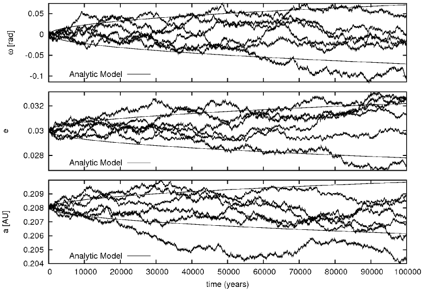
Figure 1: Time evolution of the longitude of periastron $\varpi$, the eccentricity $e$ and the semi major axis $a$ for a single planet. The initial orbital parameters of the planet were taken to be those of GJ876 b (see table 1). Six different realisations starting from the same initial conditions are shown in each panel. The diffusion coefficients are $D=8.2\cdot 10^{-5}{\mbox{cm}^{2}}/{\mbox{s}^{3}}$ for the upper three panels and $D=8.2\cdot 10^{-3}{\mbox{cm}^{2}}/{\mbox{s}^{3}}$ for the lower three respectively. The solid lines correspond to the analytic predictions for the amount of spreading (see text).

3.4 Illustration of the Modes of Libration in a Two Planet System

We now go on to consider two planet systems. As an illustrative example we consider the GJ876 system (see table 1). Note that we can easily scale all physical quantities and extend the discussion to other systems (see section 6 for a discussion). We begin by considering the evolution of the system without stochastic forcing in order to characterize the modes of libration of the resonant angles and other orbital parameters. In particular we identify the fast and slow modes discussed in section 2.2.2.

The time evolution of the resonant angles and the eccentricities is plotted in figure 2. Clearly visible are the slow and fast oscillation modes. The fast mode, which is seen to have a period of about 1.4 years, dominates the librations of $e_{2}$, and $\phi_{1}$ while also being present in those of $\phi_{2}.$ On the other hand the slow mode, which is seen to have a period of about 10 years, dominates the librations of $\zeta$ while also being present in those of $e_{1}$ and $\phi_{2}.$

We emphasize the fact that the eccentricities of the two planets participate in the librations and so are not constant. In particular, the eccentricity of GJ876 b oscillates around a mean value of $0.03$ with an amplitude $\Delta e\approx 0.01-0.02$. This behaviour involving the attainment of smaller values of the eccentricity has important consequences for stochastic evolution as discussed above (see section 2.3.3) and see also below.

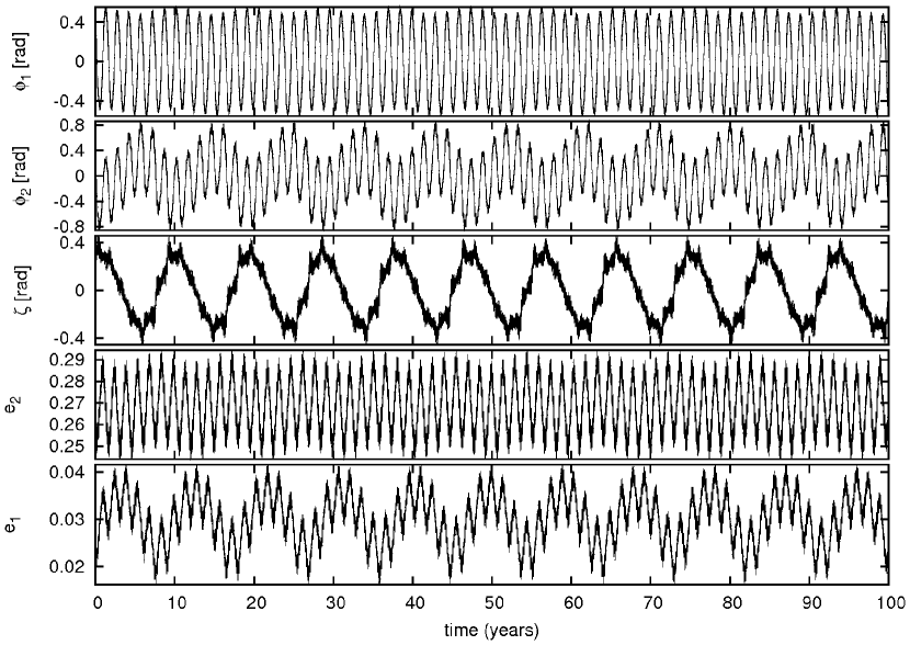
Figure 2: Time evolution of the resonant angles and the eccentricities in the system GJ876 without turbulent forcing. The dominance of the fast mode with period $\sim 1.4$ years in the oscillations of $\phi_{1}$, and the dominance of the slow mode with period $\sim 10$ years in $\zeta$ can be clearly seen.

We remark that similar behaviour occurs for all the systems we have studied, these have a wide range of eccentricities and planet masses. Indeed we note that the period scalings of the fast and slow mode periods with the planet masses are provided by equations (31) and (33) respectively. These indicate, as confirmed by our simulations, that if both masses are reduced by a factor $\Lambda$ then the period of the fast mode scales as $\sqrt{\Lambda}$ and the period of the slow mode scales as $\Lambda.$

4 Two Planets with Stochastic Forcing

We now consider systems of two planets with stochastic forcing. For simplicity we begin by applying forcing only to the outer planet. We have found that adding the same form of forcing to the inner planet tends to speed up the evolution by approximately a factor of two without changing qualitative details. For illustrative purposes we again start with the GJ876 system and consider two diffusion coefficients $D=8.2\leavevmode\nobreak\ \cdot\leavevmode\nobreak\ 10^{-5}\text{cm}^{2}/\text{s}^{3}$ and $D=8.2\leavevmode\nobreak\ \cdot\leavevmode\nobreak\ 10^{-4}\text{cm}^{2}/\text{s}^{3}$. We remark that all of our simulations were run with constant values of $D=2\langle F_{i}\rangle^{2}\tau_{c}.$ This was done maintaining the parameters $\left<F_{i}\right>$ and $\tau_{c}$ to be constant, with $\tau_{c}$ being determined for the initial location of the outer planet. For the cases considered here, there is little orbital migration so this is not a significant feature. Note also that different realizations of the system are likely to become unstable and scatter for higher values of $D$ (see below).

The time evolution of the eccentricities is plotted in figure 3. We see fast oscillations superimposed on a random walk. The amplitude of the oscilations, as well as the mean value, changes with time.

Our simple analytic model, assumes slowly changing background eccentricities and semi-major axes and accordingly does not incorporate the oscillations of the eccentricity due to the resonant interaction of the planets. In order to make a comparison, we perform a time average over many periods to get smoothed quantities whose behaviour we can compare with that expected from equations (46) - (49). When this procedure is followed, the evolution is in reasonable accord with that expected from the analytic model provided that allowance is made for the importance of small values of $e_{1}$ in determining the growth of the libration amplitude of the angle between the apsidal lines of the two planets (see equation (49)). The presence of this feature results in the behaviour of the libration amplitude being more complex than that implied by a process governed by a simple diffusive random walk.

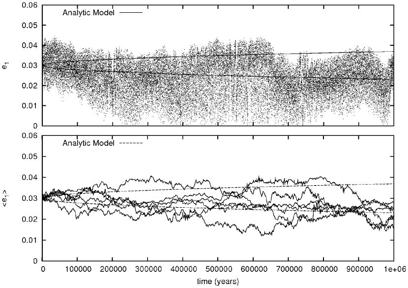
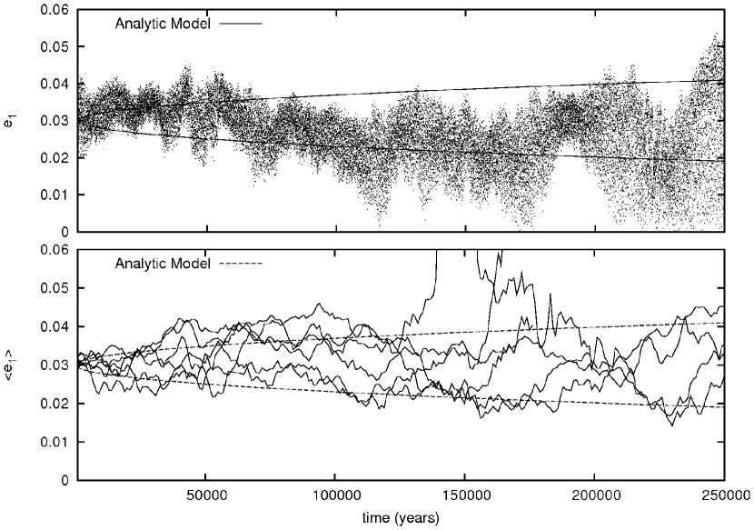
Figure 3: Time evolution of the eccentricities in the GJ876 system with turbulent forcing included. The diffusion coefficient is $D=8.2\leavevmode\nobreak\ \cdot\leavevmode\nobreak\ 10^{-5}\text{cm}^{2}/\text{s}^{3}$ for the two upper plots and $D=8.2\leavevmode\nobreak\ \cdot\leavevmode\nobreak\ 10^{-4}\text{cm}^{2}/\text{s}^{3}$ for the two lower plots. The first (uppermost) and the third plots each show a single run. The second and fourth (lowermost) plots show the time averaged eccentricity for four runs. The averaging interval is 1000 years.

4.1 Disruption of a Resonance in Stages

Systems with mean motion commensurabilities can be in many different configurations. Here we describe the important evolutionary stages as they appear in a stochastically forced system that starts from a situation in which all the resonant angles show small amplitude libration. For example observations of GJ876 suggest that the system is currently in such a state with the ratio of the orbital periods $P_{1}/P_{2}$ oscillating about a mean value of $2.$

4.1.1 Attainment of Circulation of the Angle Between the Apsidal Lines

When the initial eccentricity of the outer planet, $e_{1},$ is small the excitation of the libration amplitudes of the resonant angles readily brings about a situation where $e_{1}$ attains very small values. This causes the periastron difference $\zeta$ to undergo large oscillations and eventually circulation (see equation (49)). Should stochastic forces cause $e_{1}$ to reach zero, on account of the coordinate singularity $\varpi_{1}$ becomes undefined. Subsequently very small perturbations are able to produce a small eccentricity with $\zeta$ undergoing large amplitude librations or circulation (see below). But note that as also mentioned in section 2.1, this occurs without a large physical perturbation to the system. Thus the occurence of this phenomenon does not imply the system ceases to be in a commensurability.

In this context we note that the eccentricity of GJ876 b initially is such that $e_{1}\sim 0.03$ with values $e_{1}\sim 0.01$ often being attained during libration cycles. Thus only a small change may cause the above situation to occur. In all cases we have considered, we find that $\zeta$ enters circulation prior to the fast angle $\phi_{1},$ which may remain librating until that too is driven into circulation.

4.1.2 Attainment of Circulation of the Fast Angle

Both before and after $\zeta$ enters circulation, stochastic forcing acts to increase the libration amplitude of the fast mode. This mode dominates both the librations of the resonant angle $\phi_{1}$ and the semi major axes. Eventually $\phi_{1}$ starts circulation. Shortly afterwards commensurability is lost and $P_{1}/P_{2}$ starts to undergo a random walk with a centre that drifts away from 2. Note that it is possible for some realizations to re-enter commensurability. For systems with the masses of the observed GJ876 system, the most likely outcome is a scattering event that causes complete disruption of the system.

4.1.3 A Numerical Illustration

In order to illustrate the evolutionary sequence described above we plot results for two realisations of the evolution of the GJ876 system in figure 4. For these runs we adopted the diffusion coefficient $D=0.42\text{cm}^{2}/\text{s}^{3}.$ In this context we note that reducing $D$ increases the evolutionary time which has been found, both analyticaly and numerically to be $\propto\leavevmode\nobreak\ 1/D$ (see below).

The times at which the transition from libration to circulation occurs for both the slow and fast angles are indicated by the vertical lines in figure 4.

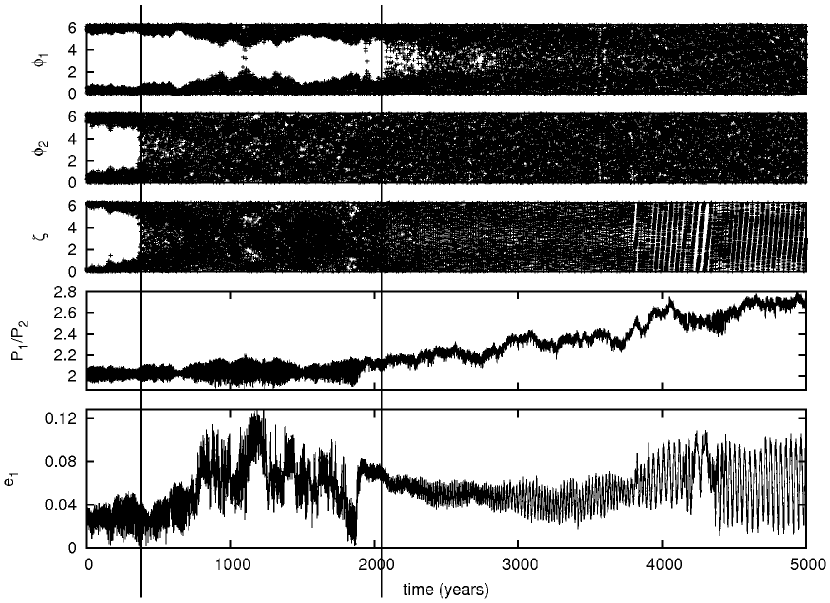
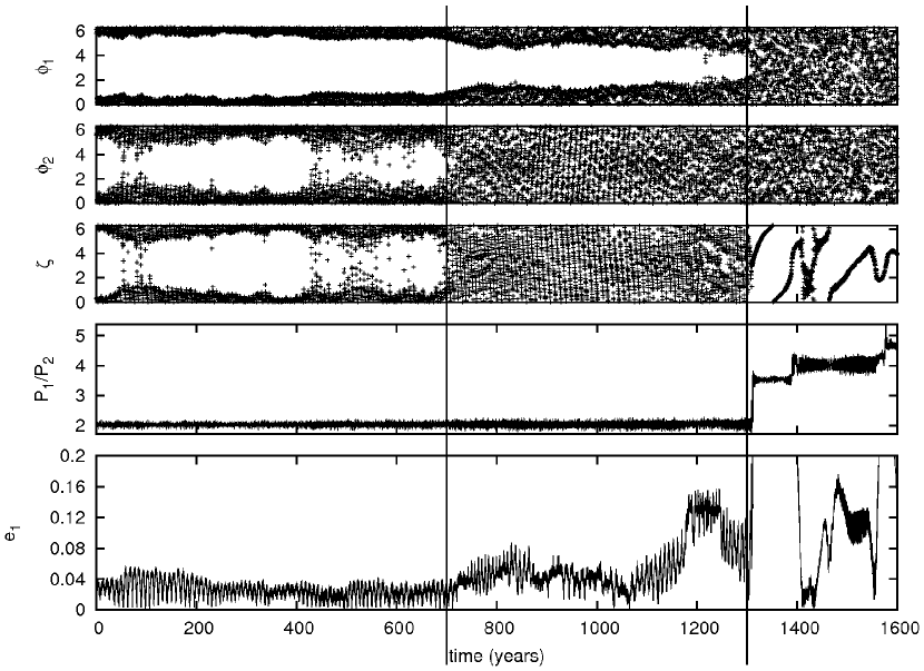
Figure 4: Time evolution of the resonant angles, the period ratio $P_{2}/P_{1}$ and the eccentricity, $e_{1},$ in the GJ876 system with stochastic forcing corresponding to $D=0.42\text{cm}^{2}/\text{s}^{3}$. The vertical lines indicate when the angles enter circulation for a prolonged period. The realisation illustrated in the lower panel scatters shortly after $\phi_{1}$ goes into circularization.

Several of the features discussed above and in section 2.3.3 can be seen in figure 4. In particular the tendency for the occurence of very small values of $e_{1}$ to be associated with transitions to circulation of $\zeta$ can be seen for the realisation plotted in the lower panels at around $t=80$ years and $t=500$ years. Such episodes always seem to occur when the libration amplitude of the fast angle $\phi_{1}$ is relatively boosted, indicating that this plays a role in boosting the slow angle. If the period of time for which $e_{1}$ attains small values is small and $\phi_{1}$ recovers small amplitude librations, the slow angle returns to circulation. Thus the attainment of long period circulation for the slow angle is related to the diffusion time for $\phi_{1}.$ We also see from figure 4 that the angle $\phi_{2},$ which has a large contribution from the slow mode, behaves in the same way as $\zeta$ as far as libration/circularization is concerned. We have verified by considering the results from the simulations of GJ876 LM HE, which started with a larger value of $e_{1},$ that, as expected, the attainment of circulation of the slow angle takes relatively longer in this case, the time approaching more closely the time when $\phi_{1}$ attains circulation. Also as expected, the time when $\phi_{1}$ attains circulation is not affected by the change in $e_{1}$.

4.2 Dependence on the Diffusion Coefficient

We now consider the stability of the systems listed in table 1 as a function of $D.$ These systems have a variety of masses and orbital eccentricities. In particular, in view of the complex interaction between the resonant angles discussed above we wish to investigate whether the mean amplitude growth at a given time is indeed proportional to $D.$ As also mentioned above, the value of the diffusion parameter $D,$ that should be adopted, is very uncertain. We have therefore considered values of $D$ ranging over five orders of magnitude. However, the correlation time $\tau_{c}$ is always taken to be given by $\tau_{c}=0.5\Omega^{-1}$ while the RMS value of the force is changed. In order to determine the ”lifetime” of a resonant angle, we monitor whether it is librating or circulating. Numerically, libration is defined to cease at the first time the angle is seen to reach absolute values largen than $2$. We note that the angle can in general regain small values afterwards. However, this is a transient effect and changes the lifetime by no more than a factor of $\sim 2$ in all our simulations.

In this context we consider the fast angle $\phi_{1}$ and the slow angle $\zeta,$ though, as we saw above, the latter can be replaced by $\phi_{2}$ which exhibits the same behaviour. As $\phi_{1}$ is the last to start circulating the resonance is defined to be broken at that point.

Equations (60) and (59) estimate the spreading of the resonant angles as a function of time. We determine the times to attain circulation as the times to attain $(\Delta\phi_{i})^{2}=4,i=1,2$ assuming the initial values for the orbital elements. We plot both the numerical and analytical results in figure 5. To remove statistical fluctuations and obtain a mean spreading time, the numerical values for a particular value of $D$ were obtained by averaging over $60$ realizations.

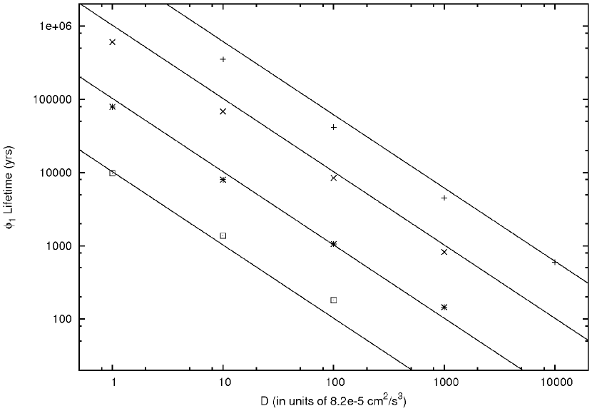
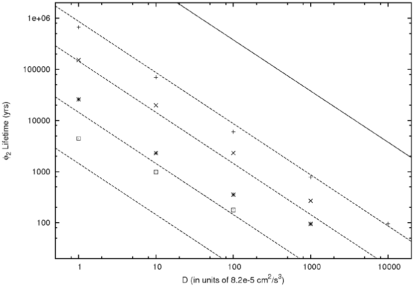
Figure 5: Average time until circulation of the resonant angles $\phi_{1}$ (top) and $\phi_{2}$ (bottom) in the GJ876 (indicated with $+$) , GJ876LM (indicated with $\times$), GJ876SE (indicated with $\star$) and GJ876E (indicated with $\Box$) systems as a function of the stochastic forcing diffusion coefficient $D.$ In the case of the upper panel, the analytic curves explained in the text, are from top to bottom for the GJ876, GJ876LM, GJ876SE and GJ876E systems respectively. In the lower panel the analytic curves, as explained in the text, are from top to bottom for the GJ876 (solid curve and top dashed curve), GJ876LM, GJ876SE and GJ876E systems respectively.

From figure 5 it is apparent that the evolutionary times scale is $\propto 1/D$ for $D$ varying by many orders of magnitude. The analytic estimates for the libration survival times of $\phi_{1},$ dominated by the fast mode, obtained using equation (60) adopting the initial orbital elements and with the fast libration frequency determined from the simulations, are plotted in the upper panel of figure 5. These are in good agreement with the numerical results. However, the estimate for $\phi_{2}$ based on equation (59) using the initial value of $e_{1}$ overestimates the lifetime by a factor of at least $\sim 40$ (see solid line in the lower plot of figure 5). Futhermore (59) has no dependence on planet mass which is in clear conflict with the numerical results. This, as discussed above is due to the temporary attainment of small eccentricities. This causes the disruption of the libration of $\zeta$ earlier than would be predicted assuming $e_{1}$ is constant. In fact this disruption occurs at times that can be up to a factor of $10$ times shorter than those required to disrupt $\phi_{1}$. We estimate the lifetime of librations of $\phi_{2}$ by calculating the time $\phi_{1}$ needs to reach values close to $1$ (see dashed lines in the lower plot of figure 5). As explained above in section 2.3.3, large amplitude variations of $\phi_{1}$ are expected to couple to and excite the slow mode. Variations induced in the eccentricity $e_{1}$ allow this to reach zero and we lose libration of $\phi_{2}.$ These simple estimates are in good agreement with the numerical results and accordingly support the idea that $\phi_{1}$ and $\phi_{2}$ are indeed coupled in the non linear regime. For low mass planets this simple analytic prediction underestimates the lifetime of $\phi_{2}$ by a factor of $\sim 2$, suggesting that the coupling between the two modes depends slightly on the planet masses.

To confirm our understanding of these processes, we have repeated the calculations with systems that are in the same state as the system discussed above but have higher eccentricities (see GJ876 LM HE and GJ876 SE HE in table 1). The lifetime of the librating state of $\phi_{1}$ is unchanged, as this does not depend significantly on the eccentricity. However, the lifetime of the librating state of $\phi_{2}$ is a factor of $2-3$ longer. This is due to the fact that a larger excitation of $\phi_{2}$ is needed to make $e_{1}$ reach small values in these simulations.

The random walk description breaks down completely when the anticipated disruption time becomes shorter than the libration period. This is expected to happen for small enough masses as can be verified from figure 5. It is because the disruption time decreases linearly with the planet masses while the libration period increases as the square root of the planet masses. Then we cannot average over many libration periods. This situation is apparent in figure 5 for very short disruption times of the order 100-1000 years where survival times cease to vary linearly with $1/D$.

5 Formation of HD128311

We here discuss the application of the ideas discussed above to understanding the orbital configuration of the planetary system HD128311. This is (with 99% confidence) in a 2:1 mean motion resonance with the angle $\phi_{1}$ librating and the angle $\zeta$ circulating so that there is no apsidal corotation (Vogt et al. 2005). However, the orbital parameters are not well constrained. The orgininal Keplerian fit by Vogt et al. (2005) is such that the planets undergo a close encounter after only 2000 years. The values in table 1 have been obtained from a fit to the observational data that includes interactions between the planets. The values quoted have large error bars. For example the eccentricities $e_{1}$ and $e_{2}$ have an uncertainty of 33% and 21%, respectively. Although the best fit doesn’t manifest apsidal corotation, the system could undergo large amplitude librations and still be stable.

According to Lee & Peale (2002) the planets should have apsidal corotation if the commensurability was formed by the two planets undergoing sufficently slow convergent inward migration, and if they then both migrated inwards significantly while maintaining the commensurability (see also Snellgrove et al. 2001). Accordingly Sándor & Kley (2006) suggested a possible formation scenario with inward migration as described above, but with an additional perturbing event, such as a close encounter with an additional planet occuring after the halting of the inward migration. This perturbation is needed to alter the behaviour of $\zeta,$ so that it undergoes circulation rather than libration and thus producing orbital parameters similar to the observed ones.

We showed above that stochastic forcing possibly resulting from turbulence driven by the MRI readily produces systems with commensurabilities without apsidal corotation if the eccentricities are not too large. This suggests that a scenario that froms the commensurability through disk induced inward convergent migration might readily produce commensurable systems without apsidal corotation if stochastic forcing is included. Such scenarios are investigated in this section.

We present simulations of the formation of HD128311 that include migration and stochastic forcing due to turbulence but do not invoke special perturbation events involving additional planets. We find that model systems with orbital parameters resembling the observed ones are readily produced that give better matches than so far provided by Sándor & Kley (2006). The planets in this system are of the order of several Jupiter masses and the eccentricity of one planet can get very small during one libration period. The observed orbital parameters are given in table 1 and plotted on the right hand side of figures 6, 7 and 8. The mass of the star is $0.8\leavevmode\nobreak\ {\rm M}_{\odot}$.

5.1 Migration Forces

We incorporate the non-conservative forces excerted by a protostellar disk that lead to inward migration by following the approach of Lee & Peale (2001) and Snellgrove et al. (2001). In this the migration process is characterized by migration and eccentricity damping timescales, $\tau_{a}={a}/{\dot{a}}$ and $\tau_{e}={e}/{\dot{e}}$. We also define the ratio of the above timescales to be $K=\left|\tau_{a}\right|/\tau_{e}$. This ratio determines the eccentricities in the state of self similar inward migration of the commensurable system that is attained after large times. We verify this result for two different values of $K$ (see below). The procedure is now widely used (e.g. Sándor & Kley 2006; Crida et al. 2008) and we have checked our code against the results of their work.

In this work we allow the planets to form a commensurability through convergent inward migration but stochastic forcing is included, the disk is then removed through having its surface density reduced to zero on a 2000 year timescale. This simultaneously reduces both the migration forces and the stochastic forcing to zero. This procedure is very similar to that adopted by the above authors but we have included stochastic forcing and removed the disk on longer time scales.

The stochastic forces have to have the right balance with respect to the migration rate. We have found that inward migration imparts stability to the resonant system. If the migration rate is too fast relative to the stochastic forcing the migration keeps down the libration amplitudes and we do not get circulation. On the other hand large eccentricity damping favours broken apsidal corotation. This might look counterintuitive at first sight, but remember that the diffusion of $\zeta$ depends on $1/e^{2}_{1,2}$. Due to the stochastic nature of the problem, it is hard to present a continuum of solutions so we restrict ourselves to the discussion of three representative examples. However, we comment that we are able to obtain similar end states for a wide range of migration parameters. Before presenting these examples we briefly indicate how the librations can be stabilized by the migration process.

As above, the parameters $\left<F_{i}\right>$ and $\tau_{c}$ are kept constant, so maintaining $D$ constant, for the duration of the simulation, with $\tau_{c}$ being determined for the initial location of the outer planet. As discussed above, these values may scale with the radius of the planet and we thus expect them to change during migration. However, the semi major axis of the outer planet changes only by $\sim 30$ % during the simulation consequently we ignore this effect.

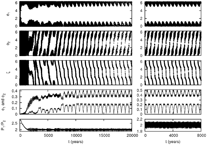
Figure 6: The plots on the left hand side show a possible formation scenario of HD128311. We plot the observed system on the right hand side as a comparison (see table 1 and text). The plots show the resonant angles $\phi_{1},\phi_{2},\zeta$, the eccentricities $e_{1},e_{2}$ and period ratio $P_{1}/P_{2}$ for formation scenarios including turbulence and migration. Resonace capturing occurs after 2000 years.

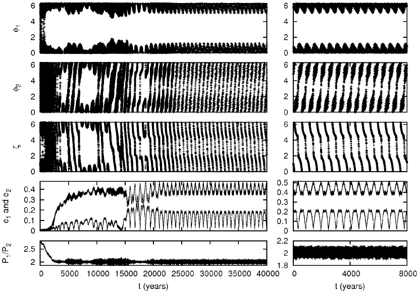
Figure 7: The plots on the left hand side show another possible formation scenario of HD128311. Again, we plot the observed system on the right hand side as a comparison (see table 1 and text. The migration timescales in this run are $\tau_{a,1}=16000$, $\tau_{a,2}=-40000$ and $K=5.5$. Note that the eccentricities are larger compared to figure 6 because $K$ is smaller.

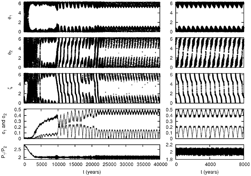
Figure 8: These plots show another possible formation scenario of HD128311. The damping parameters are the same as in figure 7.

5.2 Adiabatic Invariance and the Stabilization of Librations through Damping

Both the fast angle $\phi_{1}$ and the slow angle $\phi_{2}$ obey stochastically forced oscillator equations. Although we do not have a simple expressions for the oscillation frequencies we know that for fixed eccentricity and planet masses they both scale as the orbital frequency, $n_{1}.$ When the planets migrate inwards together, this increases slowly with time. Accordingly the theory of adiabatic invariance indicates that the libration amplitude should scale as $n_{1}^{-1/2}$ (Peale 1976). If there were no stochastic forcing or other effects, the libration amplitude would decrease on twice the migration time scale $2\tau_{a}$ once steady eccentricities were formed. This provides only a small effect given the typical amount of migration $\sim 30\%$ in our simulations.

A comparison of the behaviour of a model of the GJ876 system undergoing convergent orbital migration resulting in the fomation of a commensurabilty both with and without eccentricity damping was undertaken by Lee & Peale (2001). Small libration amplitudes at a similar level are attained in both models. The case without eccentricity damping attains higher eccentricities and somewhat larger libration amplitudes as the evolution continues whereas a low steady libration amplitude is maintained in the case with eccentricity damping. The above situation is consistent with the initial reduction in libration amplitude that occurs prior to the attainment of steady eccentricities as not being due to eccentricity damping but the operation of adiabatic invariance (Peale 1976).

However, a study of simulations of the GJ876 system without stochastic forcing reveals that eccentricty damping does play a role in damping the slow mode (associated with apsidal corotation) on the eccentricity damping timescale, whereas the fast mode appears to be only marginally affected at least at small amplitudes. Thus the residual librations in these cases consist mainly if not entirely of the fast mode. Therefore the inclusion of eccentricity damping does impart some stability to the commensurability through control of the slow mode and thus its possible interactions with the fast mode. As the slow mode involves $\zeta$ and $e_{1},$ (see figure 2), it is not surprising that this is affected by eccentricity damping.

Note too that because the migration process itself causes libration amplitude reduction on formation of the commensurability some stability is also implied towards some types of disturbance that would take the system away from resonance.

5.3 Model 1

The planets are initially in circular orbits at radii $a_{1}=4$ AU and $a_{2}=2$ AU. Stochastic forcing is applied to the outer planet only with the diffusion coefficient $D=6.4\cdot 10^{-3}\text{cm}^{2}/\text{s}^{3}.$ Note that although this value is 640 times larger than the scaling given by equation (65), corresponding to a force that is 25 times larger than the simple estimate given in section 3.1, corresponding to smaller reduction factors resulting from a gap or dead zone, it is too small for the angle $\phi_{1}$ to be brought to circulation during our runs. The results given above and summarized in figure 5, and other tests, indicate that similar results would be obtained if $D$ is reduced, but on a longer time scale $\propto 1/D,$ provided the migration rate is also appropriately ultimately reduced so that the system can survive for long enough to enable $\zeta$ to be driven into circulation.

The outer planet is made to migrate inwards on a timescale $\tau_{a_{1}}=8000$ years. The inner planet migrated slowly outwards on a timescaly of $\tau_{a_{2}}=-20000$ years. This results in convergent migration. For both planets we use an eccentricity to semi major axis damping ratio of $K=8$. The resulting evolutionary timescales are significantly larger than those used by eg. Sándor & Kley (2006) and more easily justified by hydrodynamical simulations.

The time evolution is shown in the left plot of figure 6. After resonance capturing all angles are either initially librating or on the border between libration and circulation. The slow mode has a period of $\sim 700$ years, whereas the slow mode period is 20 times shorter.

It can be seen from figure 6 and other related figures below, that while migration continues libration ampliudes tend to be controlled apart from when $e_{1}$ becomes either zero or very close to zero. Then, due to stochastic forcing, $\phi_{2}$ and $\zeta$ start circulating. Subsequently libration is recovered over time intervals for which $e_{1}$ does not attain very small values but eventually additional stochastic forcing together with the repeated attainment of small values for $e_{1}$ causes $\phi_{2}$ to remain circulating for the remainder of the simulation. After $13000$ years, both the forces due to migration and turbulence are reduced smoothly on a timescale of $2000$ years. The result is a stable configuration that resembles the observed system very well.

5.4 Model 2

For this simulation, we lengthened the migration timescales by a factor of 2 to show that the results are generic. We also decreased the value of $K$ to $5.5$. This results in larger eccentricities and the final state better resembled our representation of the observed system. However, it should be kept in mind that the eccentricities are not well constrained by the observations. All other parameters are the same as for model 1. The time evolution is plotted in figure 7. The resonant angles librate immediately after the capture into resonance as predicted for sufficiently slow migration. However, in the same way as for model 1 described above, stochastic forces make $\phi_{2}$ circulate soon afterwards. Once the migration forces and stochastic forces are removed between $20000$ and $22000$ years, the system stays in a stable configuration with no apsidal corotation.

5.5 Model 3

All parameters are the same as for model 2. Accordingly model 3 represents another statistical realization of that case. The time evolution is plotted in figure 8. The final state is very close to the boundary between libration and circulation of $\zeta.$ As discussed above, large uncertainties in the orbital parameters means that the actual system could be in such a state.

Due to stochastic forces, which may result from local turbulence, we are able to generate a broad spectrum of model systems. Some of them undergo a strong scattering during the migration process. However, the surving systems resemble the observed system very well. Although the orbital parameters are not well constrained yet, we showed that values in the right range are naturally produced by a turbulent disk.

6 Discussion

In this paper, we have presented a self consistent analytic model applicable to either a single planet or two planets in a mean motion resonance subject to external stochastic forcing. The stochastic forces could result from MRI driven turbulence within the protoplanetary disk but our treatment is equally applicable to any other source.

We considered the evolution of a stochasticly forced two planet system that is initially deep inside a MMR (ie. the two independent resonant angles librate with small amplitude). Stochastic forces cause libration amplitudes to increase in the mean with time until all resonant angles are driven into circulation at which point the commensurability is lost. Often a strong scattering occurs soon afterwards for sytems composed of planets in the Jovian mass range.

We isolated a fast libration mode which is associated with oscillations of the semi-major axes and a slow libration mode which is mostly associated with the motion of the angle between the apsidal lines of the two planets. These modes respond differently to stochastic forcing, the slow mode being more readily converted to circulation than the fast mode. This slow mode is sensitive to the attainment of small eccentricities which cause rapid transitions between libration and circulation. The amplitude of the fast mode grows more regularly in the mean, with the square of the libration amplitude in most cases increasing linearly with time and being proportional to the diffusion coefficient $D$. Of course this discussion is simplified and there are limitations. For example if the total mass of the system is reduced, the disruption time eventually becomes comparable to the libration period. In that case the averaging process that we used in the derivation is no longer valid and the lifetime no longer scales as $1/D.$

The analytic model was compared with numerical simulations which incorporated stochastic forces. Those forces, parameterized by the mean square values of each component in cylindrical ccoordinates and the autocorrelation time, were applied in a continuous manner giving results that could be directly compared with the analytic model. The simulations were in broad agreement with analytic predictions and we presented illustrative examples of the disruption process. We performed the simulations for a large range of diffusion parameters, planet masses and initial eccentricities to verify the scaling law for the commensurability disruption time summarized hereafter.

To summarize our results, recalling that the slow angle is driven into circulation before the fast angle, so that the ultimate lifetime is determined by the time taken for the fast angle to achieve circulation, we determine the lifetime, $t_{f},$ using equation (60) setting $t=t_{f},$ $(\Delta Q)^{2}=(\Delta Q)^{2}_{0}=4,$ together with $\gamma_{f}=p=1,$ so obtaining

$$t_{f} = \frac{a_{1}^{2}\omega_{lf}^{2}(\Delta Q)^{2}_{0}}{36D}.$$ (69)

We showed above that this gives good agreement with our numerical results. Using $D=2\langle F_{i}^{2}\rangle\tau_{c},$ we can express this result in terms of the relative magnitude of the stochastic forcing in the form

$$t_{f} = 2.4\times 10^{-4}\left(\frac{a_{1}^{2}n_{1}^{4}}{\langle F_{i}^{2}\rangle}\right)\left(\frac{(\Delta Q)^{2}_{0}}{8n_{1}\tau_{c}}\right)$$ (70)

$$\;\;\cdot\left(\frac{8.5\omega_{lf}\sqrt{q_{GJ}}}{n_{1}\sqrt{q}}\right)^{2}\frac{q}{q_{GJ}}P_{1},$$

where $P_{1}$ is the orbital period of the outer planet. Here the first quantity in brackets represents the ratio of the square of the central force per unit mass to the mean square stochastic force per unit mass acting on the outer planet. The other quantities in brackets, scaled to the GJ876 system are expected to be unity, while the last factor $q/q_{GJ}$ is the ratio of the total mass ratio of the system to the same quantity for GJ876. Here it is assumed that the two planets in the system have comparable masses.

From (70) we see that a non migrating system such as GJ876 could survive in resonance for $t_{f}\sim 10^{6}$ years if the stochastic force amplitude is $\sim 10^{-5}$ times the central force. This expression enables scaling to other systems at other disk locations for other stochastic forcing amplitudes. Inference of survival probabilities for particular systems depends on many uncertain aspects, such as the protoplanetary disk model and the strength of MRI turbulence. However, the mass ratio dependence in equation (70) indicates that survival is favored for more massive systems. At the present time the number of observed resonant systems is too small for definitive conclusions to be made. However, the fact that several systems exhibiting commensurabilities have been observed indicates that resonances are not always completely disrupted by stochastic forces due to turbulence, but rather may be modified as in our study of HD128311.

The HD128311 system is such that the fast mode librates with the slow mode being near the borderline between libration and circulation. We found that such a configuration was readily produced in a scenario in which the commensurability was formed through a temporary period of convergent migration with the addition of stochastic forcing. During a migration phase moderate adiabatic invariance applied to the libration modes together with eccentricity damping leads to increased stabilization and a longer lifetime for the resonance. However, as discussed above, the time evolution of the eccentricity and in particular the attainment of small values plays an important role in causing the slow mode to circulate corresponding to the loss of apsidal corotation. Thus we expect that a large eccentricity damping rate does not necessarily stabilize the apsidal corotation of the system. Additional simulations have shown that this is lost more easily for large damping rates ($K\gg 10$). On the other hand it should be noted that this has less significance when one of the orbits becomes nearly circular.

Further observations of extrasolar planetary systems leading to better statistics may lead to an improved situation for assessing the role of stochastic forcing in future.