Measures and Dimensions of Julia sets of Semi-hyperbolic Rational Semigroups

Abstract.

We consider the dynamics of semi-hyperbolic semigroups generated by finitely many rational maps on the Riemann sphere. Assuming that the nice open set condition holds it is proved that there exists a geometric measure on the Julia set with exponent $h$ equal to the Hausdorff dimension of the Julia set. Both $h$-dimensional Hausdorff and packing measures are finite and positive on the Julia set and are mutually equivalent with Radon-Nikodym derivatives uniformly separated from zero and infinity. All three fractal dimensions, Hausdorff, packing and box counting are equal. It is also proved that for the canonically associated skew-product map there exists a unique $h$-conformal measure. Furthermore, it is shown that this conformal measure admits a unique Borel probability absolutely continuous invariant (under the skew-product map) measure. In fact these two measures are equivalent, and the invariant measure is metrically exact, hence ergodic.

Mathematics Subject Classification (2001). Primary 37F35; Secondary 37F15.

1. Introduction

In this paper, we frequently use the notation from [36]. A “rational semigroup” $G$ is a semigroup generated by a family of non-constant rational maps $g:\hat{\mathbb{C}}\rightarrow\hat{\mathbb{C}}$, where $\hat{\mathbb{C}}$ denotes the Riemann sphere, with the semigroup operation being functional composition. For a rational semigroup $G$, we set

$$F(G):=\{z\in\hat{\mathbb{C}}\mid G\mbox{ is normal in a neighborhood of }z\}$$

and

$$J(G):=\hat{\mathbb{C}}\setminus F(G).$$

$F(G)$ is called the Fatou set of $G$ and $J(G)$ is called the Julia set of $G.$ If $G$ is generated by a family $\{f_{i}\}_{i}$, then we write $G=\langle f_{1},f_{2},\ldots\!\rangle.$

The work on the dynamics of rational semigroups was initiated by Hinkkanen and Martin ([15]), who were interested in the role of the dynamics of polynomial semigroups while studying various one-complex-dimensional moduli spaces for discrete groups, and by F. Ren’s group ([54]), who studied such semigroups from the perspective of random complex dynamics. The theory of the dynamics of rational semigroups on $\hat{\mathbb{C}}$ has developed in many directions since the 1990s ([15, 54, 16, 28, 29, 30, 31, 34, 35, 36, 37, 38, 39, 40, 41, 49, 42, 43, 44, 45, 32, 46]).

Since the Julia set $J(G)$ of a rational semigroup $G$ generated by finitely many elements $f_{1},\ldots\!\!,f_{u}$ has backward self-similarity, i.e.,

(1.1) $$J(G)=f_{1}^{-1}(J(G))\cup\cdots\cup f_{u}^{-1}(J(G))$$

(see [36]), it can be viewed as a significant generalization and extension of both, the theory of iteration of rational maps (see [23]), and conformal iterated function systems (see [22]). For example, the Sierpiński gasket can be regarded as the Julia set of a rational semigroup. The theory of the dynamics of rational semigroups borrows and develops tools from both of these theories. It has also developed its own unique methods, notably the skew product approach (see [36, 37, 38, 39, 42, 43, 44, 45, 49], and [50]). We remark that by (1.1), the analysis of the Julia sets of rational semigroups somewhat resembles “backward iterated functions systems”, however since each map $f_{j}$ is not in general injective (critical points), some qualitatively different extra effort in the cases of semigroups is needed.

The theory of the dynamics of rational semigroups is intimately related to that of the random dynamics of rational maps. For the study of random complex dynamics, the reader may consult [13, 4, 5, 3, 2, 14, 24]. We remark that the complex dynamical systems can be used to describe some mathematical models. For example, the behavior of the population of a certain species can be described as the dynamical system of a polynomial $f(z)=az(1-z)$ such that $f$ preserves the unit interval and the postcritical set in the plane is bounded (cf. [10]). From this point of view, it is very important to consider the random dynamics of polynomials. For the random dynamics of polynomials on the unit interval, see [33].

The deep relation between these fields (rational semigroups, random complex dynamics, and (backward) IFS) is explained in detail in the subsequent papers ([40, 41, 42, 43, 44, 45, 46, 47, 48]) of the first author.

In this paper, we investigate the Hausdorff, packing, and box dimension of the Julia sets of semi-hyperbolic rational semigroups $G=\langle f_{1},\ldots,f_{u}\rangle$ satisfying the nice open set condition. We will show that these dimensions coincide, that $0<\mbox{H}^{h}(J(G)),\mbox{P}^{h}(J(G))<\infty$, where $h$ is the Hausdorff dimension of $J(G)$ and $\mbox{H}^{h}$ (resp. $\mbox{P}^{h}$) denotes the $h$-dimensional Hausdorff (resp. packing) measure, that $h$ is equal to the critical exponent of the Poincaré series of the semigroup $G$, that there exists a unique $h$-conformal measure $\tilde{m}_{h}$ on the Julia set $J(\tilde{f})$ of the “skew product map” $\tilde{f}$, that there exists a unique Borel probability measure $\tilde{\mu}_{h}$ on $J(\tilde{f})$ which is absolutely continuous with respect to $\tilde{m}_{h}$, and that $\tilde{\mu}_{h}$ is metrically exact and equivalent with $\tilde{m}_{h}$. The precise statements of these results are given in Theorem  1.11. In order to prove these results, we develop and combine the idea of usual iteration of non-recurrent critical point maps ([51]), conformal iterated function systems ([22]), and the dynamics of expanding rational semigroups ([38]). However, as we mentioned before, since the generators may have critical points in the Julia set, we need some careful treatment on the critical points in the Julia set and some observation on the overlapping of the backward images of the Julia set under the elements of the semigroup.

Our approach develops the methods from [38], [51], and [52]. In order to prove that a conformal measure exists, is atomless, and, ultimately, geometric, we expand the concepts of estimability of measures, which originally appeared in [51], we introduce a partial order in the set of critical points, and a stratification of invariant subsets of the Julia set. As an entirely new tool to all [38], [51], and [52], we introduce the concept of essential families of inverse branches. This concept, supported by the notion of nice open set, is extremely useful in the realm of semi-hyperbolic rational semigroups, at it would also (without nice open set) substantially simplified considerations in the expanding case.

In the second part of the paper, devoted to proving the existence and uniqueness of an invariant (with respect to the canonical skew-product) probability measure equivalent with the $h$-conformal measure, the most challenging task is to prove the uniqueness of the latter. We do it by bringing up and elaborating the tool of Vitali relations due to Federer (see [12]), the tool which has not come up in [51], [52] nor [38]. We rely here heavily on deep results from [12]. The second tool, already employed in [52] and subsequent papers of the second author, is the Marco Martens method of producing $\sigma$-finite invariant measures absolutely continuous with respect to a given quasi invariant measure. We apply and develop this method, proving in particular its validity for abstract measure spaces and not only for $\sigma$-compact measure spaces. This is possible because of our use of Banach limits rather than weak convergence of measures.

We remark that as illustrated in [41, 40, 47], estimating the Hausdorff dimension of the Julia sets of rational semigroups plays an important role when we investigate random complex dynamics and its associated Markov process on $\hat{\mathbb{C}}.$ For example, when we consider the random dynamics of a compact family $\Gamma$ of polynomials of degree greater than or equal to two, then the function $T_{\infty}:\hat{\mathbb{C}}\rightarrow[0,1]$ of probability of tending to $\infty\in\hat{\mathbb{C}}$ varies only on the Julia set of rational semigroup generated by $\Gamma$, and under some condition, this $T_{\infty}:\hat{\mathbb{C}}\rightarrow[0,1]$ is continuous on $\hat{\mathbb{C}}$ and varies precisely on $J(G).$ If the Hausdorff dimension of the Julia set is strictly less than two, then it means that $T_{\infty}:\hat{\mathbb{C}}\rightarrow[0,1]$ is a complex version of devil’s staircase (Cantor function) ([40, 41, 47, 48]).

In order to present the precise statements of the main result, we give some basic notations. For each meromorphic function $\varphi$, we denote by $|\varphi^{\prime}(z)|_{s}$ the norm of the derivative with respect to the spherical metric. Moreover, we denote by $CV(\varphi)$ the set of critical values of $\varphi.$

Given a set $A\subset{\mathbb{C}}$ and $r>0$, the symbol $B(A,r)$ denotes the Euclidean open $r$-neighborhood of the set $A$ and $\text{\rm{diam}}(A)$ denotes the diameter of $A$ with respect to the Euclidean distance. Furthermore, given a subset $A$ of $\hat{\mathbb{C}}$, $B_{s}(A,r)$ denotes the spherical open $r$-neighborhood of the set $B$, and finally $\text{\rm{diam}}_{s}(A)$ denotes the diameter of $A$ with respect to the spherical distance.

Let $u\in{\mathbb{N}}.$ In this paper, an element of $(\mbox{Rat})^{u}$ is called a multi-map.

Let $f=(f_{1},\ldots,f_{u})\in(\mbox{Rat})^{u}$ be a multi-map and let $G=\langle f_{1},\ldots\!,f_{u}\rangle$ be the rational semigroup generated by $\{f_{1},\ldots,f_{u}\}.$ Then, we use the following notation. Let $\Sigma_{u}:=\{1,\ldots\!,u\}^{\mathbb{N}}$ be the space of one-sided sequences of $u$-symbols endowed with the product topology. This is a compact metric space. Let $\tilde{f}:\Sigma_{u}\times\hat{\mathbb{C}}\rightarrow\Sigma_{u}\times\hat{\mathbb{C}}$ be the skew product map associated with $f=(f_{1},\ldots\!,f_{u})$ given by the formula

$$\tilde{f}(\omega,z)=(\sigma(\omega),\ f_{\omega_{1}}(z)),$$

where $(\omega,z)\in\Sigma_{u}\times\hat{\mathbb{C}},\ \omega=(\omega_{1},\omega_{2},\ldots\!),$ and $\sigma:\Sigma_{u}\rightarrow\Sigma_{u}$ denotes the shift map. We denote by $p_{1}:\Sigma_{u}\times\hat{\mathbb{C}}\rightarrow\Sigma_{u}$ the projection onto $\Sigma_{u}$ and $p_{2}:\Sigma_{u}\times\hat{\mathbb{C}}\rightarrow\hat{\mathbb{C}}$ the projection onto $\hat{\mathbb{C}}$. That is,

$$p_{1}(\omega,z)=\omega\ \text{ and }\ p_{2}(\omega,z)=z.$$

Under the canonical identification $p_{1}^{-1}\{\omega\}\cong\hat{\mathbb{C}}$, each fiber $p_{1}^{-1}\{\omega\}$ is a Riemann surface which is isomorphic to $\hat{\mathbb{C}}.$

Let $\Sigma_{u}^{*}:=\bigcup_{n\in{\mathbb{N}}}\{1,\ldots,u\}^{n}$ be the family of finite words over the alphabet $\{1,2,\ldots,u\}$. For every $\tau\in\Sigma_{u}^{*}$, we denote by $|\tau|$ the only integer $n\geq 0$ such that $\tau\in\{1,\ldots,u\}^{n}.$ For every $\tau\in\Sigma_{u}$ we set $|\tau|=\infty.$ In addition, for every $\tau=(\tau_{1},\tau_{2},\ldots)\in\Sigma_{u}^{\ast}\cup\Sigma_{u}$ and $n\in{\mathbb{N}}$ with $n\leq|\tau|$, we set

$$\tau|_{n}:=(\tau_{1},\tau_{2},\ldots,\tau_{n})\in\Sigma_{u}^{\ast}.$$

For every $\tau\in\Sigma_{u}^{\ast}$, we denote

$$\hat{\tau}=\tau|_{|\tau|-1},\ \tau_{\ast}:=\tau_{|\tau|}$$

and

(1.2) $$[\tau]:=\{\omega\in\Sigma_{u}\mid\omega|_{|\tau|}=\tau\}$$

Furthermore, for every $\omega\in\Sigma_{u}^{\ast}\cup\Sigma_{u}$ and all $a,b\in{\mathbb{N}}$ with $a<b\leq|\omega|$, we set

$$\omega_{a}^{b}:=(\omega_{a},\ldots,\omega_{b})\in\Sigma_{u}^{\ast}.$$

For all $\omega,\tau\in\Sigma_{u}^{\ast}$, we say that $\omega$ and $\tau$ are comparable if either (1) $|\tau|\leq|\omega|$ and $\omega\in[\tau]$, or (2) $|\omega|\leq|\tau|$ and $\tau\in[\omega].$ We say that $\omega,\tau$ are incomparable if they are not comparable. By $\tau\omega\in\Sigma_{u}^{\ast}$ we denoted the concatenation of the words $\tau$ and $\omega$. For each $\omega=(\omega_{1},\ldots,\omega_{n})\in\Sigma_{u}^{\ast}$, let

$$f_{\omega}:=f_{\omega_{n}}\circ\cdots\circ f_{\omega_{1}}.$$

Fix $\tau\in\Sigma_{u}^{\ast},x\in\hat{\mathbb{C}},$ and $n\in{\mathbb{N}}$. Suppose that $z=f_{\tau}(x)$ is not a critical value of $f_{\tau}.$ Then we denote by $f_{\tau,x}^{-1}$ the inverse branch of $f_{\tau}$ mapping $z$ to $x.$ Furthermore, we denote by $\tilde{f}_{\tau,x}^{-|\tau|}$ the inverse branch of $\tilde{f}^{|\tau|}$ such that $\tilde{f}_{\tau,x}^{-|\tau|}(\omega,y)=(\tau\omega,f_{\tau,x}^{-1}(y)).$ Let

$$\text{{\rm Crit}}(\tilde{f}):=\bigcup_{\omega\in\Sigma_{u}}\{v\in p_{1}^{-1}\{\omega\}\mid v\mbox{ is a critical point of }\tilde{f}|_{p_{1}^{-1}\{\omega\}}\rightarrow p_{1}^{-1}\{\sigma(\omega)\}\}\ (\subset\Sigma_{u}\times\hat{\mathbb{C}})$$

be the set of critical points of $\tilde{f}.$ For each $n\in{\mathbb{N}}$ and $(\omega,z)\in\Sigma_{u}\times\hat{\mathbb{C}}$, we set

$$(\tilde{f}^{n})^{\prime}(\omega,z):=(f_{\omega_{n}}\circ\cdots\circ f_{\omega_{1}})^{\prime}(z).$$

For each $\omega\in\Sigma_{u}$ we define

$$J_{\omega}:=\{z\in\hat{\mathbb{C}}\mid\{f_{\omega_{n}}\circ\cdots\circ f_{\omega_{1}}\}_{n\in{\mathbb{N}}}\mbox{ is not normal in any neighborhood of }z\}$$

and we then set

$$J(\tilde{f}):=\overline{\cup_{w\in\Sigma_{u}}\{\omega\}\times J_{\omega}},$$

where the closure is taken in the product space $\Sigma_{u}\times\hat{\mathbb{C}}.$ By definition, $J(\tilde{f})$ is compact. Furthermore, by Proposition 3.2 in [36], $J(\tilde{f})$ is completely invariant under $\tilde{f}$, $\tilde{f}$ is an open map on $J(\tilde{f})$, $(\tilde{f},J(\tilde{f}))$ is topologically exact under a mild condition, and $J(\tilde{f})$ is equal to the closure of the set of repelling periodic points of $\tilde{f}$ provided that $\sharp J(G)\geq 3$, where we say that a periodic point $(\omega,z)$ of $\tilde{f}$ with period $n$ is repelling if the modulus of the multiplier of $f_{\omega_{n}}\circ\cdots\circ f_{\omega_{1}}$ at $z$ is strictly larger than $1$. Furthermore,

$$p_{2}(J(\tilde{f}))=J(G).$$

Definition 1.1.

Let $G$ be a rational semigroup and let $F$ be a subset of $\hat{\mathbb{C}}.$ We set $G(F)=\bigcup_{g\in G}g(F)$ and $G^{-1}(F)=\bigcup_{g\in G}g^{-1}(F).$ Moreover, we set $G^{\ast}=G\cup\{Id\}$, where $Id$ denotes the identity map on $\hat{\mathbb{C}}.$ Furthermore, let $E(G):=\{z\in\hat{\mathbb{C}}\mid\#\bigcup_{g\in G}g^{-1}(\{z\})<\infty\}.$

Proposition 1.2 (Proposition 3.2(f) in [36]).

(topological exactness) Let $G=\langle f_{1},\ldots,f_{u}\rangle$ be a finitely generated rational semigroup. Suppose $\#J(G)\geq 3$ and $E(G)\subset F(G).$ Then, the action of the semigroup $G$ on the Julia set $J(G)$ is topologically exact, meaning that for every non-empty open set $U\subset J(G)$ there exist $g_{1},g_{2},\ldots,g_{n}\in G$ such that

$$g_{1}(U)\cup g_{2}(U)\cup\ldots g_{n}(U)\supset J(G).$$

Definition 1.3.

A rational semigroup $G$ is called semi-hyperbolic if and only if there exists an $N\in{\mathbb{N}}$ and a $\delta>0$ such that for each $x\in J(G)$ and $g\in G$,

$$\deg(g:V\rightarrow B_{s}(x,\delta))\leq N$$

for each connected component $V$ of $g^{-1}(B_{s}(x,\delta)).$

Definition 1.4.

Let $f=(f_{1},\ldots,f_{u})\in(\mbox{{\em Rat}})^{u}$ be a multi-map and let $G=\langle f_{1},\ldots,f_{u}\rangle.$ We say that $G$ (or $f$) satisfies the open set condition if there exists a non-empty open subset $U$ of $\hat{\mathbb{C}}$ with the following two properties:

• $f_{1}^{-1}(U)\cup f_{2}^{-1}(U)\cup\ldots f_{u}^{-1}(U)\subset U$,

• $f_{i}^{-1}(U)\cap f_{2}^{-1}(U)=\emptyset$ whenever $i\neq j$.

Moreover, we say that $G$ (or $f$) satisfies the nice open set condition if in addition the following condition is satisfied.

• $\exists(\alpha\in(0,1))\,\forall(0<r\leq 1)\,\forall(x\in\overline{U})\ \ l_{2}(U\cap B_{s}(x,r))\geq\alpha l_{2}(B_{s}(x,r))$, where $l_{2}$ denotes the $2$-dimensional Lebesgue measure on $\hat{\mathbb{C}}.$

Remark 1.5.

Condition (osc3) is not needed if our semigroup $G$ is expanding (see [38] or note that our proofs would use only (osc1) and (osc2) under this assumption). Condition (osc3) is satisfied in the theory of conformal infinite iterated function systems (see [21], comp. [22]), where it follows from the open set condition and the cone condition. Moreover, condition (osc3) holds for example if the boundary of $U$ is smooth enough; piecewise smooth with no exterior cusps suffices. Furthermore, (osc3) holds if $U$ is a John domain (see [6]).

Definition 1.6 ([38]).

Let $G$ be a countable rational semigroup. For any $t\geq 0$ and $z\in\hat{\mathbb{C}}$, we set $S_{G}(z,t):=\sum_{g\in G}\sum_{g(y)=z}|g^{\prime}(y)|_{s}^{-t}$, counting multiplicities. We also set $S_{G}(z):=\inf\{t\geq 0:S_{G}(z,t)<\infty\}$ (if no $t$ exists with $S_{G}(z,t)<\infty$, then we set $S_{G}(z):=\infty$). Furthermore, we set $s_{0}(G):=\inf\{S_{G}(z):z\in\hat{\mathbb{C}}\}.$ This $s_{0}(G)$ is called the critical exponent of the Poincaré series of $G.$

Definition 1.7 ([38]).

Let $f=(f_{1},\ldots,f_{u})\in(\mbox{{\em Rat}})^{u}$, $t\geq 0$, and $z\in\hat{\mathbb{C}}.$ We put $T_{f}(z,t):=\sum_{\omega\in\Sigma_{u}^{\ast}}\sum_{f_{\omega}(y)=z}|f_{\omega}^{\prime}(y)|_{s}^{-t}$, counting multiplicities. Moreover, we set $T_{f}(z):=\inf\{t\geq 0:T_{f}(z,t)<\infty\}$ (if no $t$ exists with $T_{f}(z,t)<\infty$, then we set $T_{f}(z)=\infty$). Furthermore, we set $t_{0}(f):=\inf\{T_{f}(z):z\in\hat{\mathbb{C}}\}.$ This $t_{0}(f)$ is called the critical exponent of the Poincaré series of $f=(f_{1},\ldots,f_{u})\in(\mbox{{\em Rat}})^{u}.$

Remark 1.8.

Let $f=(f_{1},\ldots,f_{u})\in(\mbox{{\em Rat}})^{u}$, $t\geq 0$ , $z\in\hat{\mathbb{C}}$ and let $G=\langle f_{1},\ldots,f_{u}\rangle.$ Then, $S_{G}(t,z)\leq T_{f}(t,z),S_{G}(z)\leq T_{f}(z),$ and $s_{0}(G)\leq t_{0}(f).$ Note that for almost every $f\in(\mbox{{\em Rat}})^{u}$ with respect to the Lebesgue measure, $G=\langle f_{1},\ldots,f_{u}\rangle$ is a free semigroup and so we have $S_{G}(t,z)=T_{f}(t,z),S_{G}(z)=T_{f}(z),$ and $s_{0}(G)=t_{0}(f).$

Definition 1.9.

Let $\varphi:J(\tilde{f})\rightarrow{\mathbb{R}}$ be a function. Let $\nu$ be a Borel probability measure on $J(\tilde{f}).$ We say that $\nu$ is a $\varphi$-conformal measure for the map $\tilde{f}:J(\tilde{f})\rightarrow J(\tilde{f})$ if for each Borel subset $A$ of $J(\tilde{f})$ such that $\tilde{f}|_{A}:A\rightarrow J(\tilde{f})$ is injective, we have

$$\nu(\tilde{f}(A))=\int_{A}\varphi\ d\nu.$$

A $|\tilde{f}^{\prime}|_{s}^{t}$-conformal measure $\nu$ is sometimes called a $t$-conformal measure. When $J(G)\subset{\mathbb{C}}$, a $|\tilde{f}^{\prime}|^{t}$-conformal measure is also sometimes called a $t$-conformal measure.

Definition 1.10.

Let $G=\langle f_{1},\ldots,f_{u}\rangle$ and let $t\geq 0.$ For all $z\in\hat{\mathbb{C}}\setminus G^{\ast}(\bigcup_{j=1}^{u}\text{CV}(f_{j}))$, we set

$$P_{z}(t):=\limsup_{n\rightarrow\infty}\frac{1}{n}\log\sum_{|\omega|=n}\sum_{x\in f_{\omega}^{-1}(z)}|f_{\omega}^{\prime}(x)|_{s}^{-t}.$$

The main result of this paper is the following.

Theorem 1.11 (see Lemma 7.2, Lemma 7.3, Theorem 7.16, Corollary 7.18 and Theorem 8.4).

Let $f=(f_{1},\ldots,f_{u})\in(\mbox{{\em Rat}})^{u}$ be a multi-map. Let $G=\langle f_{1},\ldots,f_{u}\rangle$. Suppose that there exists an element $g$ of $G$ such that $\deg(g)\geq 2$, that each element of Aut$(\hat{\mathbb{C}})\cap G$ (if this is not empty) is loxodromic, that $G$ is semi-hyperbolic, and that $G$ satisfies the nice open set condition. Then, we have the following.

• $J(G)\cap\overline{G^{\ast}(\bigcup_{j=1}^{u}\text{CV}(f_{j}))}$ is nowhere dense in $J(G)$ and, for each $t\geq 0$, the function $z\mapsto P_{z}(t)$ is constant throughout a neighborhood of $J(G)\setminus\overline{G^{\ast}(\bigcup_{j=1}^{u}\text{CV}(f_{j}))}$ in $\hat{\mathbb{C}}.$ Denote this constant by $P(t)$.

• The function $t\mapsto P(t)$ has a unique zero. This zero is denoted by $h=h(f)$.

• There exists a unique $|\tilde{f}^{\prime}|_{s}^{h}$-conformal measure $\tilde{m}_{h}$ for the map $\tilde{f}:J(\tilde{f})\rightarrow J(\tilde{f}).$

• Let $m_{h}:=\tilde{m}_{h}\circ p_{2}^{-1}.$ Then there exists a constant $C\geq 1$ such that

  $$C^{-1}\leq\frac{m_{h}(B_{s}(z,r))}{r^{h}}\leq C$$

  for all $z\in J(G)$ and all $r\in(0,1].$

• $h(f)=\text{{\rm HD}}(J(G))=\text{{\rm PD}}(J(G))=\text{{\rm BD}}(J(G))$, where $\text{{\rm HD}},\text{{\rm PD}},\text{{\rm BD}}$ denote the Hausdorff dimension, packing dimension, and box dimension, respectively, with respect to the spherical distance in $\hat{\mathbb{C}}.$ Moreover, for each $z\in J(G)\setminus\overline{G^{\ast}(\bigcup_{j=1}^{u}\text{CV}(f_{j}))}$, we have $h(f)=T_{f}(z)=t_{0}(f)=S_{G}(z)=s_{0}(G).$

• Let $\text{{\rm H}}^{h}$ and $\text{{\rm P}}^{h}$ be the $h$-dimensional Hausdorff dimension and $h$-dimensional packing measure respectively. Then, all the measures $\text{{\rm H}}^{h},\text{{\rm P}}^{h}$, and $m_{h}$ are mutually equivalent with Radon-Nikodym derivatives uniformly separated away from zero and infinity.

• $0<\text{{\rm H}}^{h}(J(G)),\text{{\rm P}}^{h}(J(G))<\infty.$

• There exists a unique Borel probability $\tilde{f}$-invariant measure $\tilde{\mu}_{h}$ on $J(\tilde{f})$ which is absolutely continuous with respect to $\tilde{m}_{h}.$ The measure $\tilde{\mu}_{h}$ is metrically exact and equivalent with $\tilde{m}_{h}.$

The proof of Theorem 1.11 will be given in the following Sections 2–8. In Section 9, we give some examples of semi-hyperbolic rational semigroups satisfying the nice open set condition.

ACKNOWLEDGMENT: We wish to thank the anonymous referee for his/her valuable comments and suggestions which improved the final exposition of our paper.

2. Preliminaries

2.1. Distortion and Measures

All the points (numbers) appearing in this paper are complex unless it is clear from the context that they are real. In particular $x$ and $y$ are always assumed to be complex numbers and not the real and imaginary parts of a complex number.

Theorem 2.1.

(Koebe’s ${1\over 4}$-Theorem) If $z\in{\mathbb{C}}$, $r>0$ and $H:B(z,r)\to{\mathbb{C}}$ is an arbitrary univalent analytic function, then $H(B(z,r))\supset B(H(z),4^{-1}|H^{\prime}(z)|r)$.

Theorem 2.2.

(Koebe’s Distortion Theorem, I) There exists a function $k:[0,1)\to[1,\infty)$ such that for any $z\in{\mathbb{C}}$, $r>0$, $t\in[0,1)$ and any univalent analytic function $H:B(z,r)\to{\mathbb{C}}$ we have that

$$\sup\{|H^{\prime}(w)|:w\in B(z,tr)\}\leq k(t)\inf\{|H^{\prime}(w)|:w\in B(z,tr)\}.$$

We put $K=k(1/2)$.

The following is a straightforward consequence of these two distortion theorems.

Lemma 2.3.

Suppose that $D\subset{\mathbb{C}}$ is an open set, $z\in D$ and $H:D\to{\mathbb{C}}$ is an analytic map which has an analytic inverse $H_{z}^{-1}$ defined on $B(H(z),2R)$ for some $R>0$. Then for every $0\leq r\leq R$

$$B(z,K^{-1}r|H^{\prime}(z)|^{-1})\subset H_{z}^{-1}(B(H(z),r))\subset B(z,Kr|H^{\prime}(z)|^{-1}).$$

We also use the following more geometric versions of Koebe’s Distortion Theorems involving moduli of annuli.

Theorem 2.4.

(Koebe’s Distortion Theorem, II) There exists a function $w:(0,+\infty)\to[1,\infty)$ such that for any two open topological disks $Q_{1}\subset Q_{2}\subset{\mathbb{C}}$ with $\text{{\em Mod}}(Q_{2}\setminus Q_{1})\geq t$ and any univalent analytic function $H:Q_{2}\to{\mathbb{C}}$ we have

$$\sup\{|H^{\prime}(\xi)|:\xi\in Q_{1}\}\leq w(t)\inf\{|H^{\prime}(\xi)|:\xi\in Q_{1}\}.$$

Definition 2.5.

If $H:D\to{\mathbb{C}}$ is an analytic map, $z\in{\mathbb{C}}$, and $r>0$, then by

$$\text{{\rm Comp}}(z,H,r)$$

we denote the connected component of $H^{-1}(B(H(z),r))$ that contains $z$.

Given an analytic function $H$ defined throughout a region $D\subset{\mathbb{C}}$, we put

$$\text{{\rm Crit}}(H)=\{z\in D:H^{\prime}(z)=0\}.$$

Suppose now that $c$ is a critical point of an analytic map $H:D\to{\mathbb{C}}$. Then there exists $R=R(H,c)>0$ and $A=A(H,c)\geq 1$ such that

$$A^{-1}|z-c|^{q}\leq|H(z)-H(c)|\leq A|z-c|^{q}$$

and

$$A^{-1}|z-c|^{q-1}\leq|H^{\prime}(z)|\leq A|z-c|^{q-1}$$

for every $z\in\text{{\rm Comp}}(c,H,R)$, and that

$$H(\text{{\rm Comp}}(c,H,R))=B(H(c),R),$$

where $q=q(H,c)$ is the order of $H$ at the critical point $c$. In particular

$$\text{{\rm Comp}}(c,H,R)\subset B(c,(AR)^{1/q}).$$

Moreover, by taking $R>0$ sufficiently small, we can ensure that the above two inequalities hold for every $z\in B(c,(AR)^{1/q})$ and the ball $B(c,(AR)^{1/q})$ can be expressed as a union of $q$ closed topological disks with piecewise smooth boundaries and mutually disjoint interiors such that the map $H$ restricted to each of these interiors, is injective.

In the sequel we require the following technical lemma proven in [51] as Lemma 2.11.

Lemma 2.6.

Let $H:D\rightarrow{\mathbb{C}}$ be an analytic function. Suppose that an analytic map $Q\circ H:D\to\mathbb{C}$, a radius $R>0$ and a point $z\in D$ are such that

$$\text{{\rm Comp}}(H(z),Q,2R)\cap\text{{\rm Crit}}(Q)=\emptyset\ \text{{\rm and }}\ \text{{\rm Comp}}(z,Q\circ H,R)\cap\text{{\rm Crit}}(H)\neq\emptyset.\ \ \mbox{{\em(a)}}$$

If $c$ belongs to the last intersection, $A=A(H,c),$ and $q$ is the order of $H$ at $c$, and

$$\text{\rm{diam}}\bigl{(}\text{{\rm Comp}}(z,Q\circ H,R)\bigr{)}\leq(AR(H,c))^{1/q},\ \ \ \ \ \ \ \ \ \ \ \ \ \ \ \ \ \ \ \ \ \ \ \ \ \ \ \ \ \ \ \ \ \ \ \ \ \ \ \ \mbox{{\em(b)}}$$

then

$$|z-c|\leq KA^{2}|(Q\circ H)^{\prime}(z)|^{-1}R.$$

Proof. In view of Lemma 2.3

$$\text{{\rm Comp}}(H(z),Q,R)\subset B(H(z),KR|Q^{\prime}(H(z))|^{-1}).$$

So, since $H(c)\in\text{{\rm Comp}}(H(z),Q,R)$, we get

$$H(c)\in B(H(z),KR|Q^{\prime}(H(z))|^{-1}).$$

Thus, using this and (b) we obtain

$$A^{-1}|z-c|^{q} \leq|H(z)-H(c)|$$

$$\leq KR|Q^{\prime}(H(z))|^{-1}$$

$$=KR|(Q\circ H)^{\prime}(z)|^{-1}|H^{\prime}(z)|$$

$$\leq KR|(Q\circ H)^{\prime}(z)|^{-1}A|z-c|^{q-1}.$$

So, $|z-c|\leq KA^{2}|(Q\circ H)^{\prime}(z)|^{-1}R$. $\square$

Developing the appropriate concepts from [51] we now shall define the notions of estimabilities (upper, lower and strongly lower) of measures, and we shall prove some of its properties and consequences.

Definition 2.7.

Suppose $m$ is a finite Borel measure on Borel set $X\subset{\mathbb{R}}^{n}$.

• (Upper Estimability) The measure $m$ is said to be upper $t$-estimable at a point $x\in X$ if there exist $L>0$ and $R>0$ such that

  $$m(B(x,r))\leq Lr^{t}$$

  for all $0\leq r\leq R$. The number $L$ is referred to as the upper estimability constant of the measure $m$ at $x$ and the number $R$ is referred to as the upper estimability radius of the measure $m$ at $x$. If there exists an $L>0$ and an $R>0$ such that the measure $m$ is upper $t$-estimable at each point of $X$ with the upper estimability constant $L$ and the upper estimability radius $R$, the measure $m$ is said to be uniformly upper $t$-estimable.

• (Lower Estimability) The measure $m$ is said to be lower $t$-estimable at a point $x\in X$ if there exists an $L>0$ and an $R>0$ such that

  $$m(B(x,r))\geq Lr^{t}$$

  for all $0\leq r\leq R$. The number $L$ is referred to as the lower estimability constant of the measure $m$ at $x$ and the number $R$ is referred to as the lower estimability radius of the measure $m$ at $x$. If there exists an $L>0$ and an $R>0$ such that the measure $m$ is lower $t$-estimable at each point of $X$ with the lower estimability constant $L$ and the lower estimability radius $R$, then the measure $m$ is said to be uniformly lower $t$-estimable.

• (Strongly Lower Estimability) The measure $m$ is said to be strongly lower $t$-estimable at a point $x\in X$ if there exists an $L>0$, a $\lambda\in(0,\infty)$, and an $R>0$ such that

  $$m(B(y,\lambda r))\geq Lr^{t}$$

  for every $y\in B(x,R)$ for all $0\leq r\leq R$. The number $L$ is referred to as the lower estimability constant of the measure $m$ at $x$, the number $R$ is referred to as the lower estimability radius of the measure $m$ at $x$, and $\lambda$ is referred to as the lower estimability size of the measure $m$ at $x$. If there exists an $L>0$, a $\lambda$, and an $R>0$ such that the measure $m$ is strongly lower $t$-estimable at each point of $X$ with the lower estimability constant $L$, the lower estimability radius $R$, and the lower estimability size $\lambda$, then the measure $m$ is said to be uniformly strongly lower $t$-estimable.

Suppose $U$ and $V$ are open subsets of ${\mathbb{C}}$, $z$ is a point of $U$, and $H:U\to V$ is an analytic map. Fix $t\geq 0$. A pair $(m_{1},m_{2})$ of finite Borel measures respectively on $U$ and $V$ is called upper $t$-conformal for $H$ if and only if

$$m_{2}(H(A))\geq\int_{A}|H^{\prime}|^{t}dm_{1}$$

for all Borel sets $A\subset U$ such that the restriction $H|_{A}$ is injective. The pair $(m_{1},m_{2})$ is called $t$-conformal if the above inequality sign can be replaced by equality. We will need the following lemmas.

Lemma 2.8.

Suppose $U$ and $V$ are open subsets of ${\mathbb{C}}$ and $H:U\to V$ is an analytic map which has an analytic inverse $H_{z}^{-1}$ defined on $B(H(z),2R)$ for some $R>0$. Suppose $(m_{1},m_{2})$ is a $t$-conformal pair of measures for $H$. Suppose $m_{2}$ is strongly lower $t$-estimable at $H(z)$ with estimability constant $L$, estimability radius $0<r_{0}\leq R/2$, and the lower estimability size $\lambda\leq 1$. Then the measure $m_{1}$ is strongly lower $t$-estimable at $z$ with lower estimability constant $L$, lower estimability radius $K^{-1}|H^{\prime}(z)|^{-1}r_{0}$, and lower estimability size $K^{2}\lambda$.

Proof. Let $0\leq r\leq r_{0}.$ Consider $x\in B(z,K^{-1}r|H^{\prime}(z)|^{-1})$. Then by Lemma 2.3 $H(x)\in B(H(z),r)$ and therefore $m_{2}(B(H(x),\lambda r))\geq Lr^{t}$. Since

$$B(H(x),\lambda r)\subset B(H(z),2r)\subset B(H(z),R)$$

we have

$$H_{z}^{-1}\bigl{(}B(H(x),\lambda r)\bigr{)}\subset B(x,K\lambda r|H^{\prime}(z)|^{-1})=B(x,K^{2}\lambda(K^{-1}|H^{\prime}(z)|^{-1}r)).$$

Thus

$$m_{1}\bigl{(}B(x,K^{2}\lambda(K^{-1}|H^{\prime}(z)|^{-1}r))\geq K^{-t}|H^{\prime}(z)|^{-t}Lr^{t}=L(K^{-1}|H^{\prime}(z)|^{-1}r)^{t}.$$

The proof is finished. $\square$

Lemma 2.9.

Suppose $U$ and $V$ are open subsets of ${\mathbb{C}}$ and $H:U\to V$ is an analytic map. Let $c\in U$ be a critical point of $H$ of order $q$. Suppose $(m_{1},m_{2})$ is a $t$-conformal pair of measures for $H$. If $m_{2}$ is lower $t$-estimable at $H(c)$ with estimability constant $L$ and estimability radius $0<T\leq R(H,c)$, then the measure $m_{1}$ is lower $t$-estimable at $c$ with estimability constant $A(H,c)^{-2t}L$ and estimability radius $(A(H,c)T)^{1/q}$.

Proof. Put $A=A(H,c)$. Let $0<r\leq T.$ Notice that $B(H(c),r)=H(\text{{\rm Comp}}(c,H,r))$. If $x\in\text{{\rm Comp}}(c,H,r)$, then $A^{-1}|x-c|^{q}\leq|H(x)-H(c)|<r$ which implies that $x\in B(c,(Ar)^{1/q})$. Thus $B(H(c),r)\subset H(B(c,(Ar)^{1/q})$ and therefore

$$Lr^{t} \leq m_{2}(B(H(c),r))$$

$$\leq m_{2}\bigl{(}H(B(c,(Ar)^{1/q}))\bigr{)}$$

$$\leq\int_{B(c,(Ar)^{1/q})}|H^{\prime}(z)|^{t}\,dm_{1}(z)$$

$$\leq\int_{B(c,(Ar)^{1/q})}A^{t}(|z-c|^{q-1})^{t}\,dm_{1}(z)$$

$$\leq A^{t}(Ar)^{{q-1\over q}t}m_{1}(B(c,(Ar)^{1/q})).$$

So, $m_{1}(B(c,(Ar)^{1/q}))\geq A^{-2t}L((Ar)^{1/q})^{t}$. $\square$

Lemma 2.10.

Suppose $U$ and $V$ are open subsets of ${\mathbb{C}}$ and $H:U\to V$ is an analytic map. Let $c\in U$ be a critical point of $H$ of order $q$. Suppose $(m_{1},m_{2})$ is an upper $t$-conformal pair of measures for $H$ such that $m_{1}(\{c\})=0$. If $m_{2}$ is upper $t$-estimable at $H(c)$ with estimability constant $L$ and estimability radius $0<T<R(H,c)$, then the measure $m_{1}$ is upper $t$-estimable at $c$ with estimability constant $q(2A(H,c)^{2})^{t}(2^{t/q}-1)^{-1}L$ and estimability radius $(A(H,c)^{-1}T)^{1/q}$.

Proof. Put $A=A(H,c)$. Take any $0<s\leq T$. then $H(B(c,(A^{-1}s)^{1/q}))\subset B(H(c),s)$. Set $R(c,a,b)=\{z:a\leq|z-c|<b\}$ and abbreviate $R(c,2^{-1/q}(A^{-1}s)^{1/q},(A^{-1}s)^{1/q})$ to $R(c).$ Using our assumptions and the fact that the map $H$ is $q$-to-$1$ on $B(c,(A^{-1}s)^{1/q})$, we obtain

$$Ls^{t} \geq m_{2}(B(H(c),s))$$

$$\geq m_{2}\bigl{(}H(B(c,(A^{-1}s)^{1/q}))\bigr{)}$$

$$\geq q^{-1}\int_{B(c,(A^{-1}s)^{1/q})}|H^{\prime}(z)|^{t}\,dm_{1}(z)$$

$$\geq q^{-1}\int_{R(c)}|H^{\prime}(z)|^{t}\,dm_{1}(z)$$

$$\geq q^{-1}A^{-t}(2^{-1}A^{-1}s)^{{q-1\over q}t}m_{1}(R(c)).$$

So, $m_{1}\bigl{(}R(c,2^{-1/q}(A^{-1}s)^{1/q},(A^{-1}s)^{1/q})\bigr{)}\leq q2^{t(1-{1\over q})}A^{2t}L((A^{-1}s)^{1/q})^{t}$ and therefore for any $0<r\leq T$,

$$m_{1}\bigl{(}B(c,(A^{-1}r)^{1/q})\bigr{)} =m_{1}\bigl{(}\bigcup_{n=0}^{\infty}R\bigl{(}c,2^{-{n+1\over q}}(A^{-1}r)^{1/q},2^{-{n\over q}}(A^{-1}r)^{1/q})\bigr{)}$$

$$=\sum_{n=0}^{\infty}m_{1}\bigl{(}R(c,2^{-{1\over q}}(A^{-1}2^{-n}r)^{1/q},(A^{-1}2^{-n}r)^{1/q})\bigr{)}$$

$$\leq q(2^{1-{1\over q}}A^{2})^{t}L\sum_{n=0}^{\infty}(A^{-1}2^{-n}r)^{t/q}$$

$$=q(2^{1-{1\over q}}A^{2})^{t}{L\over 1-2^{-{t\over q}}}((A^{-1}r)^{1/q})^{t}$$

$$=q(2A^{2})^{t}(2^{t/q}-1)^{-1}L((A^{-1}r)^{1/q})^{t}.$$

The proof is finished. $\square$

Lemma 2.11.

Suppose $U$ and $V$ are open subsets of ${\mathbb{C}}$ and $H:U\to V$ is an analytic map. Let $c\in U$ be a critical point of $H$ of order $q$. Suppose $(m_{1},m_{2})$ is a $t$-conformal pair of measures for $H$. If $m_{2}$ is strongly lower $t$-estimable at $H(c)$ with estimability constant $L$, estimability radius $0<T<R(H,c)/3$, and lower estimability size $\lambda$. Then the measure $m_{1}$ is strongly lower $t$-estimable at $c$ with lower estimability constant $\tilde{L}=L\min\{K^{-t},(A(H,c)^{2}\lambda)^{{1-q\over q}t}\}$, lower estimability radius $(A^{-1}T)^{1/q}$, and lower estimability size $\tilde{\lambda}=(2^{q+1}KA^{2}\lambda)^{1/q}$.

Proof. As in the proof of the previous lemma put $A=A(H,c)$. Let $0<r\leq T$ and let $x\in B(c,(A^{-1}r)^{1/q})$. If $\tilde{\lambda}(A^{-1}r)^{1/q}\geq 2|x-c|$, then

$$B(x,\tilde{\lambda}(A^{-1}r)^{1/q}) \supset B(c,\tilde{\lambda}(A^{-1}r)^{1/q}/2)$$

$$=B(c,(2K)^{1/q}(A\lambda r)^{1/q})$$

$$\supset B(c,(A\lambda r)^{1/q}).$$

It follows from the assumptions that $m_{2}$ is lower $t$-estimable at $H(c)$ with lower estimability constant $\lambda^{-t}L$ and lower estimability radius $\lambda T$. Therefore, in view of Lemma 2.9 the critical point $c$ is lower $t$-estimable with lower estimability constant $A^{-2t}\lambda^{-t}L$ and lower estimability radius $(A\lambda T)^{1/q}$. Thus

(2.1) $$m_{1}\bigl{(}B(x,\tilde{\lambda}(A^{-1}r)^{1/q})\bigr{)} \geq A^{-2t}\lambda^{-t}L(A\lambda r)^{t/q}$$

$$=(A^{2}\lambda)^{{1-q\over q}t}L((A^{-1}r)^{1/q})^{t}.$$

So, suppose that

(2.2) $$\tilde{\lambda}(A^{-1}r)^{1/q}<2|x-c|.$$

Since $c$ is a critical point we have

$$|H^{\prime}(x)|\geq A^{-1}|x-c|^{q-1}\geq A^{-1}\tilde{\lambda}^{q-1}(A^{-1}r)^{q-1\over q}2^{1-q},$$

which means that

(2.3) $$\tilde{\lambda}(A^{-1}r)^{1/q} \geq A^{-1}\tilde{\lambda}^{q}A^{-1}r2^{1-q}|H^{\prime}(x)|^{-1}$$

$$=4K\lambda r|H^{\prime}(x)|^{-1}\geq K\lambda r|H^{\prime}(x)|^{-1}.$$

In view of (2.2)

$$|H(x)-H(c)|\geq A^{-1}|x-c|^{q}\geq A^{-1}2^{-q}\tilde{\lambda}^{q}A^{-1}r=2K\lambda r\geq 2\lambda r$$

which implies that

(2.4) $$H(c)\notin B(H(x),2\lambda r).$$

Since $|H(x)-H(c)|\leq A|x-c|^{q}\leq R(H,c)/3$, we have $B(H(x),2\lambda r)\subset B(H(c),R(H,c))$. So, (2.4) implies the existence of a holomorphic inverse branch $H_{x}^{-1}:B(H(x),2\lambda r)\to{\mathbb{C}}$ of $H$ which sends $H(x)$ to $x$. Since, by the assumptions, the measure $m_{2}$ is lower $t$-estimable at $H(x)$ with lower estimability constant $\lambda^{-t}L$ and lower estimability radius $\lambda r$, it follows from the proof of Lemma 2.8 that the measure $m_{1}$ is lower $t$-estimable at $x$ with lower estimability constant $K^{-2t}\lambda^{-t}L$ and lower estimability radius $K\lambda r|H^{\prime}(x)|^{-1}$. Thus, using (2.3), we get

$$m_{1}\bigl{(}B(x,\tilde{\lambda}(A^{-1}r)^{1/q})\bigr{)} \geq m_{1}\bigl{(}B(x,K^{-1}\lambda r|H^{\prime}(x)|^{-1}))$$

$$\geq K^{-2t}\lambda^{-t}L(K\lambda r|H^{\prime}(x)|^{-1})^{t}$$

$$\geq K^{-t}Lr^{t}A^{-t}|x-c|^{(1-q)t}$$

$$\geq K^{-t}L(A^{-1}r)^{t}(A^{-1}r)^{{1-q\over q}t}$$

$$=K^{-t}L((A^{-1}r)^{1/q})^{t}.$$

In view of this and (2.1) the proof is completed. $\square$

By writing $A\preceq B$ we mean that there exists a positive constant $C$ such that $A\leq CB$ for all $A$ and $B$ under consideration. Then $A\succeq B$ means that $B\preceq A$, and $A\asymp B$ says that $A\preceq B$ and $B\preceq A$.

2.2. Open Set Condition and Essential Families

In this section, starting with the open set condition, we develop the machinery of essential families of inverse branches. We first prove the following two lemmas.

Lemma 2.12.

Let $G=\langle f_{1},\ldots,f_{u}\rangle$ be a rational semigroup satisfying the nice open set condition with $U.$ Let $j\in\{1,\ldots,u\}$ and let $c\in f_{j}^{-1}(\overline{U})$ be a critical point of $f_{j}.$ Then there exist constants $\zeta_{j,c}>0,\xi_{j,c}>0,$ and $T_{j,c}>0$ such that for each $x\in B_{s}(c,\zeta_{j,c})\cap f_{j}^{-1}(\overline{U})$ and for each $0<r<T_{j,c}$, $l_{2}(f_{j}^{-1}(U)\cap B_{s}(x,r))\geq\xi_{j,c}r^{2}.$

Proof.

By conjugating $G$ by an element of Aut$(\hat{\mathbb{C}})$, we may assume that $\infty\not\in f_{j}^{-1}(\{f_{j}(c)\}).$ Let $W$ be an open neighborhood of $f_{j}(c)$ in ${\mathbb{C}}$ such that $f_{j}^{-1}(W)\subset{\mathbb{C}}.$ Let $m_{1}:=l_{2,e}|_{f_{j}^{-1}(U\cap W)}$ and $m_{2}:=l_{2,e}|_{U\cap W}$, where $l_{2,e}$ denotes the Euclidian measure on ${\mathbb{C}}.$ Then $(m_{1},m_{2})$ is a $2$-conformal pair for $f_{j}.$ By the nice open set condition, there exist constants $C>0$ and $0<R<\infty$ such that for each $y\in\overline{U}\cap W$ and for each $0<r<R$, $m_{2}(B(y,r))\geq Cr^{2}.$ By using the method of the proof of Lemma 2.11, it is easy to see that there exist constants $\zeta_{j,c}^{\prime}>0$, $\xi_{j,c}>0$ and $T_{j,c}^{\prime}>0$ such that for each $x\in B(c,\zeta_{j,c}^{\prime})\cap f_{j}^{-1}(\overline{U})$ and for each $0<r<T_{j,c}^{\prime}$, $m_{2}(B(x,r))\geq\xi_{j,c}^{\prime}r^{2}.$ Thus, the statement of our lemma holds. We are done. ∎

Combining Lemma 2.12 and Koebe’s Distortion Theorem, we immediately obtain the following lemma.

Lemma 2.13.

Let $G=\langle f_{1},\ldots,f_{u}\rangle$ be a rational semigroup satisfying the nice open set condition with $U.$ Then, there exist constants $\xi>0$ and $T>0$ such that for each $j=1,\ldots,u$ and for each $x\in f_{j}^{-1}(\overline{U})$, $l_{2}(f_{j}^{-1}(U)\cap B_{s}(x,r))\geq\xi r^{2}.$

For every family $\mathcal{F}\subset\Sigma_{u}^{*}$ let

$$\hat{\mathcal{F}}=\{{\hat{\tau}}:\tau\in{\mathcal{F}}\}\ \text{ and }\mathcal{F}_{*}=\{\tau_{*}:\tau\in{\mathcal{F}}\}.$$

Definition 2.14.

Let $G=\langle f_{1},\ldots,f_{u}\rangle$ be a rational semigroup satisfying the nice open set condition. Suppose that $J(G)\subset{\mathbb{C}}.$ Fix a number $M>0$, a number $a>0$, and $V$, an open subset of $\Sigma_{u}$. Suppose $x\in J(G)$ and $r\in(0,1]$. A family $\mathcal{F}\subset\Sigma_{u}^{*}$ is called $(M,a,V)$-essential for the pair $(x,r)$ provided that the following conditions are satisfied.

• For every $\tau\in\mathcal{F}$, $f_{\tau}(x)\in J(G).$

• For every $\tau\in\mathcal{F}$ there exists a number $R_{\tau}$ with $0<R_{\tau}<a$ and an $f_{\hat{\tau},x}^{-1}:B(f_{\hat{\tau}}(x),2R_{\tau})\to{\mathbb{C}}$, an analytic inverse branch of $f_{\hat{\tau}}^{-1}$ sending $f_{\hat{\tau}}(x)$ to $x$, such that

  $$M^{-1}R_{\tau}\leq|f_{\hat{\tau}}^{\prime}(x)|r\leq{1\over 4}R_{\tau}.$$

• The family $\mathcal{F}$ consists of mutually incomparable words.

• $\bigcup_{\tau\in\mathcal{F}}[\tau]=V$.

If $V=\Sigma_{u}$, the family $\mathcal{F}$ is simply called $(M,a)$-essential for the pair $(x,r)$.

We shall prove the following.

Proposition 2.15.

Let $G=\langle f_{1},\ldots,f_{u}\rangle$ be a rational semigroup satisfying the nice open set condition with $U.$ Suppose that $J(G)\subset{\mathbb{C}}.$ Then, for every number $M>0$ and for every $a>0$ there exists an integer $\#_{(M,a)}\geq 1$ with the following properties. If $V$ is an open subset of $\Sigma_{u}$, $x\in J(G)$, $r\in(0,1]$, and $\mathcal{F}\subset\Sigma_{u}^{*}$ is an $(M,a,V)$-essential family for $(x,r)$, then we have the following.

• $$B(x,r)\subset f_{{\hat{\tau}},x}^{-1}\bigl{(}B(f_{\hat{\tau}}(x),R_{\tau})\bigr{)}\subset\bigcup_{\gamma\in\mathcal{F}}f_{\hat{\gamma},x}^{-1}\bigl{(}B(f_{\hat{\gamma}}(x),R_{\gamma})\bigr{)}\subset B(x,KMr)$$

  for all $\tau\in\mathcal{F}$.

• $$J(\tilde{f})\cap(V\times B(x,r))\subset\bigcup_{\tau\in\mathcal{F}}\tilde{f}_{{\hat{\tau}},x}^{-|{\hat{\tau}}|}\bigl{(}p_{2}^{-1}(B(f_{\hat{\tau}}(x),R_{\tau}))\bigr{)}=\bigcup_{\tau\in\mathcal{F}}[\tau]\times f_{{\hat{\tau}},x}^{-1}\bigl{(}B(f_{\hat{\tau}}(x),R_{\tau})\bigr{)}.$$

• $\#\mathcal{F}\leq\#_{(M,a)}$.

Proof. Item (a) follows immediately from Theorem 2.1 (${1\over 4}$-Koebe’s Distortion Theorem), and Theorem 2.2. The equality part in item (b) is obvious. In order to prove the inclusion take $(\omega,z)\in J(\tilde{f})\cap(V\times B(x,r))$. By item (ess3) of Definition 2.14 there exists $\tau\in\mathcal{F}$ such that $\omega\in[\tau]$. But then, by the first in item (a), $(\omega,z)\in[\tau]\times f_{{\hat{\tau}},x}^{-1}\bigl{(}B(f_{\hat{\tau}}(x),R_{\tau})\bigr{)}$ and item (b) is entirely proved. Let us deal with item (c). By item (osc2) of Definition 1.4,

$$\{f_{\hat{\tau},x}^{-1}((f_{\tau_{\ast}}|_{B(f_{\hat{\tau}}(x),R_{\tau})})^{-1}(U))\}_{\tau\in\mathcal{F}}$$

is a family of mutually disjoint sets. Hence, using also (a), we get

(2.5) $$\Sigma_{\tau\in\mathcal{F}}l_{2}(f_{\hat{\tau},x}^{-1}((f_{\tau_{\ast}}|_{B(f_{\hat{\tau}}(x),R_{\tau})})^{-1}(U)))\leq l_{2}(B(x,KMr))=C\pi(KM)^{2}r^{2},$$

where $C>0$ is a constant independent of $r,M$, and $a.$ Let $L_{a}:=\xi\min\{(T/a)^{2},1\}$, where $\xi$ and $T$ come from Lemma 2.13. By Lemma 2.13, we obtain that for each $j=1,\ldots,u$ , for each $y\in\overline{f_{j}^{-1}(U)}$, and for each $0<b\leq a$,

(2.6) $$l_{2}(B(y,b)\cap f_{j}^{-1}(U))\geq L_{a}b^{2}.$$

It follows from Theorem 2.2, (2.6), and (ess1) that for all $\tau\in\mathcal{F}$, we have

$$l_{2}\left(f_{\hat{\tau},x}^{-1}((f_{\tau_{\ast}}|_{B(f_{\hat{\tau}}(x),R_{\tau})})^{-1}(U))\right) \geq K^{-2}|f_{\hat{\tau}}^{\prime}(x)|^{-2}l_{2}((f_{\tau_{\ast}}|_{B(f_{\hat{\tau}}(x),R_{\tau})})^{-1}(U))$$

$$\geq K^{-2}|f_{\tau}^{\prime}(x)|^{-2}l_{2}(B(f_{\hat{\tau}}(x),R_{\tau})\cap f_{\tau_{\ast}}^{-1}(U))$$

$$\geq K^{-2}|f_{\hat{\tau}}(x)|^{-2}L_{a}R_{\tau}^{2}$$

$$\geq K^{-2}16L_{a}r^{2}.$$

Combining this with (2.5) we get that $\#\mathcal{F}\leq(16L_{a})^{-1}CK^{4}\pi M^{2}$. We are done. $\square$

3. Basic Properties of semi-hyperbolic Rational Semigroups

In this section we define semi-hyperbolic rational semigroups and collect their dynamical properties, with proofs, which will be needed in the sequel.

Definition 3.1.

A rational semigroup $G$ is called semi-hyperbolic if and only if there exists an $N\in{\mathbb{N}}$ and a $\delta>0$ such that for each $x\in J(G)$ and $g\in G$,

$$\deg(g:V\rightarrow B_{s}(x,\delta))\leq N$$

for each connected component $V$ of $g^{-1}(B_{s}(x,\delta)).$

The crucial tool, which makes all further considerations possible, is given by the following semigroup version of Mane’s Theorem proved in [37].

Theorem 3.2.

Let $G=\langle f_{1},\ldots,f_{u}\rangle$ be a finitely generated rational semigroup. Assume that there exists an element of $G$ with degree at least two, that each element of Aut$(\hat{\mathbb{C}})\cap G$ (if this is not empty) is loxodromic, and that $F(G)\neq\emptyset.$ Then, $G$ is semi-hyperbolic if and only if all of the following conditions are satisfied.

• For each $z\in J(G)$ there exists a neighborhood $U$ of $z$ in $\hat{\mathbb{C}}$ such that for any sequence $\{g_{n}\}_{n=1}^{\infty}$ in $G$, any domain $V$ in $\hat{\mathbb{C}}$ and any point $\zeta\in U$, the sequence $\{g_{n}\}_{n=1}^{\infty}$ does not converge to $\zeta$ locally uniformly on $V.$

• For each $j=1,\ldots,u$, each $c\in\text{{\rm Crit}}(f_{j})\cap J(G)$ satisfies $\text{{\rm dist}}(c,G^{\ast}(f_{j}(c)))>0.$

The first author proved in [37] the following.

Theorem 3.3.

Let $G=\langle f_{1},\ldots,f_{u}\rangle$ be a semi-hyperbolic finitely generated rational semigroup. Assume that there exists an element of $G$ with degree at least two, that each element of Aut$(\hat{\mathbb{C}})\cap G$ (if this is not empty) is loxodromic, and that $F(G)\neq\emptyset.$ Then there exist $R>0$, $C>0$, and $\alpha>0$ such that if $x\in J(G)$, $\omega\in\Sigma_{u}^{\ast}$ and $V$ is a connected component of $f_{\omega}^{-1}(B_{s}(x,R))$, then $V$ is simply connected and $\text{\rm{diam}}_{s}(V)\leq Ce^{-\alpha|\omega|}$.

Throughout the rest of the paper, we assume the following:

Assumption ($\ast$):

• Let $f=(f_{1},\ldots,f_{u})\in(\mbox{Rat})^{u}$ be a multi-map and let $G=\langle f_{1},\ldots,f_{u}\rangle.$

• There exists an element $g$ of $G$ such that $\deg(g)\geq 2.$

• Each element of Aut$(\hat{\mathbb{C}})\cap G$ (if this is not empty) is loxodromic.

• $G$ is semi-hyperbolic.

• $G$ satisfies the nice open set condition.

In order to prove the main results (Theorem 1.11 etc.), in virtue of [51] and [52], we may assume that $u\geq 2.$ If $u\geq 2$, then the open set condition implies that $F(G)\neq\emptyset.$ Hence, conjugating $G$ by some element of Aut$(\hat{\mathbb{C}})$ if necessary, we may assume that $J(G)\subset{\mathbb{C}}.$ Thus, throughout the rest of the paper, in addition to the above assumption, we also assume that

• $u\geq 2$ and $J(G)\subset{\mathbb{C}}.$

Note that in Theorem 1.11, we work with the spherical distance. However, throughout the rest of the paper, we will work with the Euclidian distance. If we want to get the results on the spherical distance (and this would include the case $u=1$), then we have only to consider some minor modifications in our argument.

We now give further notation. A pair $(c,j)\in\hat{\mathbb{C}}\times\{1,2,\ldots,u\}$ is called critical if $f_{j}^{\prime}(c)=0$. The set of all critical pairs of $f$ will be denoted by $\text{CP}(f)$. Let $\text{{\rm Crit}}(f)$ be the union of $\bigcup_{j=1}^{u}\text{{\rm Crit}}(f_{j}).$ For every $c\in\text{{\rm Crit}}(f)$ put

$$c_{+}=\{f_{j}(c):(c,j)\in\text{CP}(f)\}.$$

The set $c_{+}$ is called the set of critical values of $c$. For any subset $A$ of $\text{{\rm Crit}}(f)$ put

$$A_{+}=\{c_{+}:c\in A\}.$$

For each $(c,j)\in\text{CP}(f)$ let $q(c,j)$ be the local order of $f_{j}$ at $c.$ For any set $F\subset\hat{\mathbb{C}}$, set

$$\omega_{G}(F)=\bigcap_{n=0}^{\infty}\overline{\bigcup_{|\omega|\geq n}f_{\omega}(F)}.$$

The latter is called the $\omega$-limit set of $F$ with respect to the semigroup $G$. Similarly, for every set $B\subset\Sigma_{u}\times\hat{\mathbb{C}}$,

(3.1) $$\omega(B)=\bigcap_{N=0}^{\infty}\overline{\bigcup_{n\geq N}\tilde{f}^{n}(B)},$$

and this set is called the $\omega$-limit set of $F$ with respect to the skew product map $\tilde{f}:\Sigma_{u}\times\hat{\mathbb{C}}\to\Sigma_{u}\times\hat{\mathbb{C}}$.

Given $\omega\in\Sigma_{u}^{*}$, $j\in\{1,2,\ldots,u\}$, $z\in\tilde{f}_{\omega}^{-1}(J(\tilde{f}))$ and $r>0$, we say that a critical pair $(c,j)$ sticks to $\text{{\rm Comp}}(z,f_{\omega},r)$ if $c\in\text{{\rm Comp}}(z,f_{\omega},r)$ and $j=\omega_{1}$. We then write

$$(c,j)\sim\text{{\rm Comp}}(z,f_{\omega},r).$$

Set

$$A=A_{f}:=\max\{A(f_{j},c):(c,j)\in\text{CP}(f)\}\ \text{ and }\ R_{f}:=\min\{R(f_{j},c):(c,j)\in\text{CP}(f)\}.$$

For $A$, $B$, any two subsets of a metric space put

$$\text{{\rm dist}}(A,B)=\inf\{\text{{\rm dist}}(a,b):a\in A,b\in B\}$$

and

$$\text{{\rm Dist}}(A,B)=\sup\{\text{{\rm dist}}(a,b):a\in A,b\in B\}.$$

Fix a positive $\beta$ smaller than the following four positive numbers (a)–(d).

$$\mbox{(a)}\ \min\{\text{{\rm dist}}(c,G^{\ast}(c_{+})):c\in\text{{\rm Crit}}(f)\cap J(G)\},\ \mbox{(b)}\ R_{f},\ \mbox{(c)}\ \min\{|c^{\prime}-c|:c,c^{\prime}\in\text{{\rm Crit}}(f)\cap J(G),c\neq c^{\prime}\},$$

and

$$\mbox{(d)}\ \text{{\rm dist}}(\bigcup_{j=1}^{u}CV(f_{j})\cap F(G),\ J(G)),$$

where, (a) is positive because of semi-hyperbolicity (Theorem 3.2). It immediately follows from Theorem 3.3 that there exists $\gamma\in(0,1/4)$ so small that if $g\in G^{\ast}$ and $g(x)\in J(G)$, then

(3.2) $$\text{Comp}(x,g,2\gamma)\subset{\mathbb{C}}\ \ \mbox{\ and \ }\text{\rm{diam}}(\text{{\rm Comp}}(x,g,2\gamma))<\beta.$$

We shall prove the following.

Lemma 3.4.

Fix $\eta\in(0,\beta)$, an integer $n\geq 0$ and $(\omega,z)\in J(\tilde{f})$. Suppose that for every $0\leq k\leq n-1$,

$$\text{\rm{diam}}\bigl{(}\text{{\rm Comp}}\bigl{(}f_{\omega|_{k}}(z),f_{\omega|_{k+1}^{n}},\eta\bigr{)}\bigr{)}\leq\beta.$$

Then each connected component $\text{{\rm Comp}}\bigl{(}f_{\omega|_{k}}(z),f_{\omega|_{k+1}^{n}},\eta\bigr{)}$ is stuck to by at most one critical pair $(c,j)$ of $f$; and if a critical pair $(c,j)$ sticks to a component $\text{{\rm Comp}}\bigl{(}f_{\omega|_{k}}(z),f_{\omega|^{n}_{k+1}},\eta\bigr{)}$, then $f_{j}(c)\in J(G).$ Furthermore, each critical pair of $f$ sticks to at most one of all these components $\text{{\rm Comp}}\bigl{(}f_{\omega|_{k}}(z),f_{\omega|^{n}_{k+1}},\eta)$.

Proof. The first part is obvious by the choice of $\beta$. In order to prove the second part suppose that

$$(c,\omega_{k+1})\sim\text{{\rm Comp}}\bigl{(}f_{\omega|_{k}}(z),f_{\omega|_{k+1}^{n}},\eta\bigr{)}\ \text{ and }\ (c,\omega_{l+1})\sim\text{{\rm Comp}}\bigl{(}f_{\omega|_{l}}(z),f_{\omega|_{l+1}^{n}},\eta\bigr{)}$$

with some $0\leq k<l\leq n-1$ and $\omega_{k+1}=\omega_{l+1}$. Then both $c$ and $f_{\omega|_{k+1}^{l}}(c)$ belong to $\text{{\rm Comp}}\bigl{(}f_{\omega|_{l}}(z),f_{\omega|_{l+1}^{n}},\eta\bigr{)}$, and therefore,

$$|f_{\omega|_{k+1}^{l}}(c)-c|\leq\text{\rm{diam}}\bigl{(}\text{{\rm Comp}}\bigl{(}f_{\omega|_{l}}(z),f_{\omega|_{l+1}^{n}},\eta\bigr{)}\bigr{)}\leq\beta,$$

contrary to the choice of $\beta$. $\square$

Let

$$\kappa=\Pi_{(c,j)\in\text{CP}(f)}q(c,j)^{-1}.$$

Lemma 3.5.

If $g\in G$ and $z\in g^{-1}(J(G))$, then

$${\rm Mod}\bigl{(}\text{{\rm Comp}}(z,g,2\gamma)\setminus\overline{\text{{\rm Comp}}(z,g,\gamma)}\bigr{)}\geq{\kappa\log 2\over\#\text{CP}(f)}.$$

Proof. By Lemma 3.4 there exists a geometric annulus $R\subset B(g(z),2\gamma)\setminus B(g(z),\gamma)$ centered at $g(z)$ and with modulus $\geq\log 2/\#\text{CP}(f)$ and such that $g^{-1}(R)\cap\text{{\rm Comp}}(z,g,2\gamma)\cap\text{{\rm Crit}}(f)=\emptyset$. Since covering maps increase moduli of annuli by factors at most equal to their degrees, we conclude that

$${\rm Mod}\bigl{(}\text{{\rm Comp}}(z,g,2\gamma)\setminus\overline{\text{{\rm Comp}}(z,g,\gamma)}\bigr{)}\geq{\rm Mod}(R_{g})\geq{\log 2/\#\text{CP}(f)\over\Pi_{(c,j)\in\text{CP}(f)}q(c,j)}={\kappa\log 2\over\#\text{CP}(f)},$$

where $R_{g}\subset\text{{\rm Comp}}(z,g,2\gamma)$ is the connected component of $R$ enclosing $\text{{\rm Comp}}(z,g,\gamma)$. $\square$

As an immediate consequence of this lemma and Theorem 2.4 we get the following.

Lemma 3.6.

Let $\omega\in\Sigma_{u}^{\ast}$ and suppose $f_{\omega}(z)\in J(G)$. If $0\leq k\leq|\omega|$ and the map $f_{\omega|_{k}}:\text{{\rm Comp}}(z,f_{\omega},2\gamma)\to\text{{\rm Comp}}(f_{\omega|_{k}}(z),f_{\omega|_{k+1}^{|\omega|}},2\gamma)$ is univalent, then

$${|f_{\omega|_{k}}^{\prime}(y)|\over|f_{\omega|_{k}}^{\prime}(x)|}\leq\text{const}$$

for all $x,y\in\text{{\rm Comp}}(z,f_{\omega},\gamma)$, where const is a number depending only on $\#\text{CP}(f)$ and $\kappa$.

Lemma 3.7.

Suppose that $g\in G$ and $g(z)\in J(\tilde{f})$. Suppose also that $Q^{(1)}\subset Q^{(2)}\subset B(g(z),\gamma)$ are connected sets. If $Q_{g}^{(2)}$ is a connected component of $g^{-1}(Q^{(2)})$ contained in $\text{{\rm Comp}}(z,g,\gamma)$ and $Q_{g}^{(1)}$ is a connected component of $g^{-1}(Q^{(1)})$ contained in $Q_{g}^{(2)}$, then

$${\text{\rm{diam}}\bigl{(}Q_{g}^{(1)}\bigr{)}\over\text{\rm{diam}}\bigl{(}Q_{g}^{(2)}\bigr{)}}\geq\Gamma{\text{\rm{diam}}\bigl{(}Q^{(1)}\bigr{)}\over\text{\rm{diam}}\bigl{(}Q^{(2)}\bigr{)}}$$

with some universal constant $\Gamma>0$ depending on $f$ only.

Proof. Write $g=f_{\omega}$, where $\omega\in\Sigma_{u}^{*}$ and put $n=|\omega|$. For every $0\leq j\leq n$, set

$$Q_{j}^{(1)}=f_{\omega|_{n-j}}(Q_{g}^{(1)})\ \text{ and }\ Q_{j}^{(2)}=f_{\omega|_{n-j}}(Q_{g}^{(2)}).$$

Let $1\leq n_{1}\leq\ldots\leq n_{v}\leq n$ be all the integers $k$ between $1$ and $n$ such that

$$\text{{\rm Crit}}(f_{\omega_{n-k+1}})\cap\text{{\rm Comp}}(f_{\omega|_{n-k}}(z),f_{\omega_{n-k+1}^{n}},2\gamma)\neq\emptyset.$$

Fix $1\leq i\leq v$. If $j\in[n_{i},n_{i+1}-1]$ (we set $n_{v+1}=n-1$), then by Lemma 3.6 there exists a universal constant $T>0$ such that

(3.3) $$\frac{\text{\rm{diam}}(Q_{j}^{(1)})}{\text{\rm{diam}}(Q_{j}^{(2)})}\geq T\frac{\text{\rm{diam}}(Q_{n_{i}}^{(1)})}{\text{\rm{diam}}(Q_{n_{i}}^{(2)})}.$$

Since, in view of Lemma 3.4, $v\leq\#\text{CP}(f)$, in order to conclude the proof it is enough to show the existence of a universal constant $E>0$ such that for every $1\leq i\leq u$

$$\frac{\text{\rm{diam}}(Q^{(1)}_{n_{i}})}{\text{\rm{diam}}(Q^{(2)}_{n_{i}})}\geq E\frac{\text{\rm{diam}}(Q^{(1)}_{n_{i}-1})}{\text{\rm{diam}}(Q^{(2)}_{n_{i}-1})}.$$

Indeed, let $c$ be the critical point in $\text{{\rm Comp}}(f_{\omega|_{n-n_{i}}}(z),f_{\omega|_{n_{i}+1}^{n}},2\gamma)$ and let $q$ be its order. Since both sets $Q^{(1)}_{n_{i}}$ and $Q^{(1)}_{n_{i}}$ are connected, we get for $j=1,2$ that

$$\text{\rm{diam}}(Q_{n_{i}-1}^{(j)}) \asymp\text{\rm{diam}}(Q_{n_{i}}^{(j)})\sup\{|f_{\omega_{n-n_{i}+1}}^{\prime}(x)|:x\in Q_{n_{i}}^{(j)}\}$$

$$\asymp\text{\rm{diam}}(Q_{n_{i}}^{(j)})\text{{\rm Dist}}(c,Q_{n_{i}}^{(i)}).$$

Hence

$$\frac{\text{\rm{diam}}(Q_{n_{i}}^{(1)})}{\text{\rm{diam}}(Q_{n_{i}}^{(2)})} \asymp\frac{\text{\rm{diam}}(Q_{n_{i}-1}^{(1)})}{\text{{\rm Dist}}(c,Q_{n_{i}}^{(1)})}\cdot\frac{\text{{\rm Dist}}(c,Q_{n_{i}}^{(2)})}{\text{\rm{diam}}(Q_{n_{i}-1}^{(2)})}$$

$$\geq\frac{\text{\rm{diam}}(Q_{n_{i}-1}^{(1)})}{\text{\rm{diam}}(Q_{n_{i}-1}^{(2)})}.$$

The proof is finished. $\square$

4. Partial Order in $\text{{\rm Crit}}(f)\cap J(G)$ and Stratification of $J(G)$

In this section we introduce a partial order in the critical set $\text{{\rm Crit}}(f)\cap J(G)$ and stratification of $J(G)$. They will be used to do the inductive steps in the proofs of the main theorems of our paper. We start with the following.

Lemma 4.1.

The set $\omega_{G}((\text{{\rm Crit}}(f)\cap J(G))_{+})$ is nowhere dense in $J(G)$.

Proof. Suppose on the contrary that the interior (relative to $J(G)$) of $\omega_{G}((\text{{\rm Crit}}(f)\cap J(G))_{+})$ is not empty. Then, there exists a critical point $c\in\text{{\rm Crit}}(f)\cap J(G)$ such that $\omega_{G}(c_{+})$ has non-empty interior. But then, in virtue of Proposition 1.2 there would exist finitely many elements $g_{1},g_{2},\ldots,g_{n}\in G$ such that $\omega_{G}(c_{+})\supset g_{1}(\omega_{G}(c_{+}))\cup g_{2}(\omega_{G}(c_{+}))\cup\ldots\cup g_{n}(\omega_{G}(c_{+}))\supset J(G)$. Hence $c\in\omega_{G}(c_{+})$, contrary to the non-recurrence condition (Theorem 3.2). $\square$

Now we introduce in $\text{{\rm Crit}}(f)\cap J(G)$ a relation $<$ which, in view of Lemma 4.2 below, is an ordering relation. Put

$$c_{1}<c_{2}\Leftrightarrow c_{1}\in\omega_{G}({c_{2}}_{+}).$$

Lemma 4.2.

If $c_{1}<c_{2}$ and $c_{2}<c_{3}$, then $c_{1}<c_{3}$.

Proof. Since $c_{2}\in\omega_{G}({c_{3}}_{+})$, we have $\omega_{G}({c_{2}}_{+})\subset\omega_{G}({c_{3}}_{+})$. Along with $c_{1}\in\omega_{G}({c_{2}}_{+})$ this implies that $c_{1}\in\omega_{G}({c_{3}}_{+})$, meaning that $c_{1}<c_{3}$. $\square$

Lemma 4.3.

There exists no $c\in\text{{\rm Crit}}(f)\cap J(G)$ such that $c<c$.

Proof. Indeed, $c<c$ means that $c\in\omega_{G}(c_{+})$, contrary to the non-recurrence condition. $\square$

Since the set $\text{{\rm Crit}}(f)\cap J(G)$ is finite, as an immediate consequence of this lemma and Lemma 4.2 we get the following.

Lemma 4.4.

There is no infinite linear subset of the partially ordered set $(\text{{\rm Crit}}(f)\cap\nolinebreak J(G),<\nolinebreak).$

Now define inductively a sequence $\{Cr_{i}(f)\}$ of subsets of $\text{{\rm Crit}}(f)\cap J(G)$ by setting $Cr_{0}(f)=\emptyset$ and

(4.1) $$Cr_{i+1}(f)=\left\{c\in(\text{{\rm Crit}}(f)\cap J(G))\setminus\bigcup_{j=0}^{i}Cr_{j}(f):c^{\prime}<c,\Rightarrow c^{\prime}\in\bigcup_{j=0}^{i}Cr_{j}(f)\right\}.$$

Lemma 4.5.

The following four statements hold.

• The sets $\{Cr_{i}(f)\}$ are mutually disjoint.

• $\exists_{p\geq 1}\ \forall_{i\geq p+1}\ \ Cr_{i}(f)=\emptyset$.

• $Cr_{0}(f)\cup\ldots\cup Cr_{p}(f)=\text{{\rm Crit}}(f)\cap J(G)$.

• $Cr_{1}(f)\neq\emptyset$.

Proof. By definition $Cr_{i+1}(f)\cap\bigcup_{j=0}^{i}Cr_{j}(f)=\emptyset$, whence disjointness in (a) is clear. As the set $\text{{\rm Crit}}(f)\cap J(G)$ is finite, (b) follows from (a). Take $p$ to be the minimal number satisfying (b) and suppose that $(\text{{\rm Crit}}(f)\cap J(G))\setminus\bigcup_{j=0}^{p}Cr_{j}(f)\neq\emptyset$. Take $c\in(\text{{\rm Crit}}(f)\cap J(G))\setminus\bigcup_{j=0}^{p}Cr_{j}(f)$. Since $Cr_{p+1}=\emptyset$, there would thus exist $c^{\prime}\in(\text{{\rm Crit}}(f)\cap J(G))\setminus\bigcup_{j=0}^{p}Cr_{j}(f)$ such that $c^{\prime}<c$. Iterating this procedure we would obtain an infinite sequence $c_{1}=c>c^{\prime}=c_{2}>c_{3}>\ldots$, contrary to Lemma 4.4. Now, part (d) follows from (c) and (4.1). $\square$

For every $(\tau,z)\in J(\tilde{f})$ put

$$\text{{\rm Crit}}(\tau,z)=\text{{\rm Crit}}(\tilde{f})\cap\omega(\tau,z)\ \text{ and }\ \text{{\rm Crit}}(\tau,z)_{+}=p_{2}(\text{{\rm Crit}}(\tilde{f})\cap\omega(\tau,z))_{+}.$$

Lemma 4.6.

If $(\tau,z)\in J(\tilde{f})$, then $p_{2}(\omega(\tau,z))\not\subset\overline{G^{\ast}(\text{{\rm Crit}}(\tau,z)_{+})}.$

Proof. Suppose on the contrary that

(4.2) $$p_{2}(\omega(\tau,z))\subset\overline{G^{\ast}(\text{{\rm Crit}}(\tau,z)_{+})}.$$

Consequently, $\text{{\rm Crit}}(\tau,z)\neq\emptyset$. Let $(\tau^{1},c_{1})\in\text{{\rm Crit}}(\tau,z)$. This means that $(\tau^{1},c_{1})\in\omega(\tau,z)$, and it follows from (4.2) that there exists $(\tau^{2},c_{2})\in\text{{\rm Crit}}(\tau,z)$ such that either $c_{1}\in\omega_{G}({c_{2}}_{+})$ or $c_{1}=g_{1}(c_{2})$ for some $g_{1}\in G$ of the form $f_{\omega}$ with $f_{\omega_{1}}^{\prime}(c_{2})=0$. Iterating this procedure we obtain an infinite sequence $((\tau^{j},c_{j}))_{j=1}^{\infty}$ of points in $\text{{\rm Crit}}(\tau,z)$ such that for every $j\geq 1$ either $c_{j}\in\omega_{G}({c_{j+1}}_{+})$ or $c_{j}=g_{j}(c_{j+1})$ for some $g_{j}\in G$ of the form $f_{\rho}$ with $f_{\rho_{1}}^{\prime}(c_{j+1})=0$. Consider an arbitrary block $c_{k},c_{k+1},\ldots,c_{l}$ such that $c_{j}=g_{j}(c_{j+1})$ for every $k\leq j\leq l-1$, and suppose that $l-(k-1)\geq\#(\text{{\rm Crit}}(f)\cap J(G))$. Then there are two indices $k\leq a<b\leq l$ such that $c_{a}=c_{b}$. Hence $g_{a}\circ g_{a+1}\circ\ldots\circ g_{b-1}(c_{b})=c_{a}=c_{b}$ and $(g_{a}\circ g_{a+1}\circ\ldots\circ g_{b-1})^{\prime}(c_{b})=0$. This however contradicts our assumption that the Julia set of $G$ contains no superstable fixed points. In consequence, the length of the block $c_{k},c_{k+1},\ldots,c_{l}$ is bounded above by $\#(\text{{\rm Crit}}(f)\cap J(G))$. Therefore, there exists an infinite sequence $(j_{n})_{n=1}^{\infty}$ such that $c_{j_{n}}\in\omega_{G}({c_{j_{n}+1}}_{+})$ for all $n\geq 1$. This however contradicts Lemma 4.4 and finishes the proof. $\square$

Now, for every $i=0,1,\ldots,p$, set

$$S_{i}(f)=Cr_{0}(f)\cup Cr_{1}(f)\cup\ldots\cup Cr_{i}(f).$$

Fix $i\in\{0,1,\ldots,p-1\}$ consider an arbitrary point $c^{\prime}\in\bigcup_{c\in Cr_{i+1}(f)}\omega_{G}(c_{+})\cap\text{{\rm Crit}}(f)\cap J(G)$. Then there exists $c\in Cr_{i+1}(f)$ such that $c^{\prime}\in\omega_{G}(c_{+})$ which equivalently means that $c^{\prime}<c$. Thus, by (4.1) we get $c^{\prime}\in S_{i}(f)$. So,

(4.3) $$\bigcup_{c\in Cr_{i+1}(f)}\omega_{G}(c_{+})\cap\bigl{(}(\text{{\rm Crit}}(f)\cap J(G))\setminus S_{i}(f)\bigr{)}=\emptyset.$$

Since the set $\bigcup_{c\in Cr_{i+1}(f)}\omega_{G}(c_{+})$ is compact and $(\text{{\rm Crit}}(f)\cap J(G))\setminus S_{i}(f)$ is finite, we therefore get

(4.4) $$\delta_{i}=\text{{\rm dist}}\left(\bigcup_{c\in Cr_{i+1}(f)}\omega_{G}(c_{+}),(\text{{\rm Crit}}(f)\cap J(G))\setminus S_{i}(f)\right)>0.$$

Set

$$\rho=\min\{\delta_{i}/2:i=0,1,\ldots,p-1\}$$

and for every $i=0,1,\ldots,p$ define

(4.5) $$J_{i}(G)=\{z\in J(G):\text{{\rm dist}}\bigl{(}G^{\ast}(z),(\text{{\rm Crit}}(f)\cap J(G))\setminus S_{i}(f)\bigr{)}\geq\rho\}.$$

We end this section with the following two lemmas concerning the sets $J_{i}(G)$.

Lemma 4.7.

$\emptyset\neq J_{0}(G)\subset J_{1}(G)\subset\ldots\subset J_{p}(G)=J(G)$.

Proof. Since $S_{i+1}(f)\supset S_{i}(f)$, the inclusions $J_{i}(G)\subset J_{i+1}(G)$ are obvious. Since $S_{p}(f)=\text{{\rm Crit}}(f)\cap J(G)$ (see Lemma 4.5), it holds $J_{p}(G)=J(G)$. We get from (4.4) that

$$\text{{\rm dist}}\left(\bigcup_{c\in Cr_{1}(f)}\omega_{G}(c_{+}),(\text{{\rm Crit}}(f)\cap J(G))\setminus S_{0}(f)\right)=\delta_{0}\geq 2\rho\geq\rho.$$

Thus, $\bigcup_{c\in Cr_{1}(f)}\omega_{G}(c_{+})\subset J_{0}(G)$, and since $Cr_{1}(f)\neq\emptyset$ (see Lemma 4.5), we conclude that $J_{0}(G)\neq\emptyset$. The proof is complete. $\square$

Lemma 4.8.

There exists $l=l(f)\geq 0$ so large that for all $i=0,1,\ldots,p-1$ we have

$$\bigcup_{c\in Cr_{i+1}(f)}\omega_{G}(c_{+})\cap J(G)\subset\overline{\bigcup_{|\tau|\geq l}f_{\tau}(Cr_{i+1}(f)_{+})}\cap J(G)=\overline{G^{\ast}\bigl{(}\bigcup_{|\tau|=l}f_{\tau}(Cr_{i+1}(f)_{+})\bigr{)}}\cap J(G)\subset J_{i}(G).$$

Proof. The left-hand inclusion is obvious regardless of what $l(f)$ is. The equality part of the assertion is obvious. In order to prove the right-hand inclusion fix $i\in\{0,1,\ldots,p-1\}$. By the definition of the $\omega$-limit sets of $G$ there exists $l_{i}\geq 0$ such that for every $c\in Cr_{i+1}(f)$ we have $\text{{\rm dist}}\bigl{(}\bigcup_{|\tau|\geq l_{i}}f_{\tau}(c_{+}),\bigcup_{c^{\prime}\in Cr_{i+1}(f)}\omega_{G}(c_{+}^{\prime})\bigr{)}<\delta_{i}/2$. Thus, by (4.4), $\text{{\rm dist}}\bigl{(}\bigcup_{|\tau|\geq l_{i}}f_{\tau}(c_{+}),(\text{{\rm Crit}}(f)\cap J(G))\setminus S_{i}(f)\bigr{)}>\delta_{i}/2\geq\rho$. Hence, for every $\tau\in\Sigma_{u}^{\ast}$ with $|\tau|\geq l_{i}$, we have $\text{{\rm dist}}\bigl{(}f_{\tau}(c_{+}),(\text{{\rm Crit}}(f)\cap J(G))\setminus S_{i}(f)\bigr{)}>\rho$. Thus $f_{\tau}(c_{+})\subset J_{i}(G)$. Therefore, $\bigcup_{|\tau|\geq l_{i}}f_{\tau}(c_{+})\subset J_{i}(G)$, and consequently, $\bigcup_{|\tau|\geq l_{i}}f_{\tau}(Cr_{i+1}(f)_{+})\subset J_{i}(G)$. Since $J_{i}(G)$ is a closed set, this yields that $\overline{\bigcup_{|\tau|\geq l_{i}}f_{\tau}(Cr_{i+1}(f)_{+})}\subset J_{i}(G)$. Setting $l(f)=\max\{l_{i}:i=0,1,\ldots,p-1\}$ completes the proof. $\square$

5. Holomorphic Inverse Branches.

In this section we prove the existence of suitable holomorphic inverse branches, our basic tools throughout the paper. Set

$$\text{Sing}(\tilde{f})=\bigcup_{n\geq 0}\tilde{f}^{-n}(\text{{\rm Crit}}(\tilde{f}))$$

and

$$\text{Sing}(f)=\bigcup_{g\in G^{\ast}}g^{-1}(\text{{\rm Crit}}(f)).$$

Recall that according to the formula (3.1), given a point $(\tau,z)\in\Sigma_{u}\times\hat{\mathbb{C}}$, the set $\omega(\tau,z)$ is the $\omega$-limit set of $(\tau,z)$ with respect to the skew product map $\tilde{f}:\Sigma_{u}\times\hat{\mathbb{C}}\to\Sigma_{u}\times\hat{\mathbb{C}}$.

Proposition 5.1.

For each $(\tau,z)\in J(\tilde{f})\setminus\text{Sing}(\tilde{f})$, there exists a number $\eta(\tau,z)$ with $0<\eta(\tau,z)<\gamma$, an increasing sequence $(n_{j})_{j=1}^{\infty}$ of positive integers and a point $(\hat{\tau},\hat{z})\in\omega(\tau,z)\setminus p_{2}^{-1}\bigl{(}\overline{G^{\ast}(\text{{\rm Crit}}(\tau,z)_{+})}\bigr{)}$ with the following two properties.

• $\lim_{j\to\infty}\tilde{f}^{n_{j}}(\tau,z)=(\hat{\tau},\hat{z})$,

• $\text{{\rm Comp}}\bigl{(}z,f_{\tau|_{n_{j}}},\eta(\tau,z)\bigr{)}\cap\text{{\rm Crit}}(f_{\tau|_{n_{j}}})=\emptyset$.

Proof. In view of Lemma 4.6 there exists a point $(\hat{\tau},\hat{z})\in\omega(\tau,z)$ such that $\hat{z}\notin\overline{G^{\ast}(\text{{\rm Crit}}(\tau,z)_{+})}$. Let

$$\eta={1\over 2}\text{{\rm dist}}\bigl{(}\hat{z},\overline{G^{\ast}(\text{{\rm Crit}}(\tau,z)_{+})}\bigr{)}.$$

Then there exists an infinite increasing sequence $(n_{j})_{j=1}^{\infty}$ of positive integers such that

(5.1) $$\lim_{j\to\infty}\tilde{f}^{n_{j}}(\tau,z)=(\hat{\tau},\hat{z})$$

and

(5.2) $$f_{\tau|_{n_{j}}}(z)\notin B\bigl{(}\overline{G^{\ast}(\text{{\rm Crit}}(\tau,z)_{+})},\eta\bigr{)}$$

for all $j\geq 1$. We claim that there exists $\eta(\tau,z)>0$ such that for all $j\geq 1$ large enough

$$\text{{\rm Comp}}\bigl{(}z,f_{\tau|_{n_{j}}},\eta(\tau,z)\bigr{)}\cap\text{{\rm Crit}}(f_{\tau|_{n_{j}}})=\emptyset.$$

Indeed, otherwise we find an increasing subsequence $(j_{i})_{i=1}^{\infty}$ and a decreasing to zero sequence of positive numbers $\eta_{i}<\eta$ such that

$$\text{{\rm Comp}}\bigl{(}z,f_{\tau|_{n_{j_{i}}}},\eta_{i}\bigr{)}\cap\text{{\rm Crit}}(f_{\tau|_{n_{j_{i}}}})\neq\emptyset.$$

Let $\tilde{c}_{i}\in\text{{\rm Comp}}\bigl{(}z,f_{\tau|_{n_{j_{i}}}},\eta_{i}\bigr{)}\cap\text{{\rm Crit}}(f_{\tau|_{n_{j_{i}}}})$. Then there exist $0\leq p_{i}\leq n_{j_{i}}-1$ and

(5.3) $$c_{i}\in\text{{\rm Crit}}(f_{\tau_{p_{i}+1}})$$

such that $c_{i}=f_{\tau|_{p_{i}}}(\tilde{c}_{i})$. Since $\lim_{i\to\infty}\eta_{i}=0$, it follows from Theorem 3.3 that $\lim_{i\to\infty}\tilde{c}_{i}=z$. Since $(\tau,z)\notin\bigcup_{n\geq 0}\tilde{f}^{-n}(\text{{\rm Crit}}(\tilde{f}))$, this implies that $\lim_{i\to\infty}p_{i}=+\infty$. But then, making use of Theorem 3.3 again and of the formula $(\sigma^{p_{i}}(\tau),c_{i})=\tilde{f}^{p_{i}}(\tau,\tilde{c}_{i})$, we conclude that the set of accumulation points of the sequence $((\sigma^{p_{i}}(\tau),c_{i}))_{1}^{\infty}$ is contained in $\omega(\tau,z)$. Fix $(\tau^{\infty},c)$ to be one of these accumulation points. Since $\text{{\rm Crit}}(\tilde{f})$ is closed we conclude that

(5.4) $$(\tau^{\infty},c)\in\text{{\rm Crit}}(\tau,z).$$

Since that set $\text{{\rm Crit}}(f)$ is finite, passing to a subsequence, we may assume without loss of generality that $(c_{i})_{1}^{\infty}$ is a constant sequence, so equal to $c$. Since $c=f_{\tau|_{p_{i}}}(\tilde{c}_{i})$, we get

$$\left|f_{\tau|_{n_{j_{i}}}}(z)-f_{\tau|_{p_{i}+1}^{n_{j_{i}}}}(c)\right|=\left|f_{\tau|_{n_{j_{i}}}}(z)-f_{\tau|_{n_{j_{i}}}}(\tilde{c}_{i})\right|<\eta_{i}<\eta.$$

But, looking at (5.3) and (5.4), we conclude that $f_{\tau|_{p_{i}+1}^{n_{j_{i}}}}(c)\in G^{\ast}(\text{{\rm Crit}}(\tau,z)_{+})$. We thus arrived at a contradiction with (5.2), and the proof is finished. $\square$

Corollary 5.2.

If $(\tau,z)\in J(\tilde{f})\setminus\text{Sing}(\tilde{f})$, then $\limsup_{n\to\infty}|f_{\tau|_{n}}^{\prime}(z)|=+\infty$.

Proof. Let $(n_{j})_{j=1}^{\infty}$ and $\eta(\tau,z)$ be produced by Proposition 5.1. Then, by this proposition and Theorem 3.3, the family $\left\{f_{\tau|_{n_{j}},z}^{-1}:B\bigl{(}f_{\tau|_{n_{j}}}(z),\eta(\tau,z)\bigr{)}\to{\mathbb{C}}\right\}_{j=1}^{\infty}$ of holomorphic inverse branches of $f_{\tau|_{n_{j}}}$ sending $f_{\tau|_{n_{j}}}(z)$ to $z$ is well defined and normal. As a matter of fact we mean here this family restricted to the disk $B(\hat{z},\eta(\tau,z)/2)$ and $j\geq 1$ large enough. Therefore by Theorem 3.3 again, $\lim_{j\to\infty}|f_{\tau|_{n_{j}}}^{\prime}(z)|^{-1}=0$ and we are done. $\square$

We end this section with the following. Let $\|\tilde{f}^{\prime}\|=\sup_{w\in J(\tilde{f})}|\tilde{f}^{\prime}(w)|.$

Proposition 5.3.

Fix $\theta\in(0,\min\{1,\gamma\})$. For all $(\tau,z)\in J(\tilde{f})$ and $r>0$ there exists a minimal integer $s=s(\theta,(\tau,z),r)\geq 0$ with the following properties (a) and (b).

• $|(\tilde{f}^{s})^{\prime}(\tau,z)|\neq 0$.

• Either $r|(\tilde{f}^{s})^{\prime}(\tau,z)|>||\tilde{f}^{\prime}||^{-1}$ or there exists $c\in\text{{\rm Crit}}(f_{\tau_{s+1}})$ such that $f_{\tau_{s+1}}(c)\in J(G)$ and

  $$|f_{\tau|_{s}}(z)-c|\leq\theta r|f_{\tau|_{s}}^{\prime}(z)|.$$

  In addition, for this $s$, we have

• $\theta r|f_{\tau|_{s}}^{\prime}(z)|\leq\theta<\gamma$ and

  $$\text{{\rm Comp}}\bigl{(}z,f_{\tau|_{s}},(KA_{f}^{2})^{-1}2^{-\#\text{{\rm Crit}}(f)}\theta r|f_{\tau|_{s}}^{\prime}(z)|\bigr{)}\cap\text{{\rm Crit}}(f_{\tau|_{s}})=\emptyset.$$

Proof. First note that the set of integers $(\geq 0)$ satisfying conditions (a) and (b) is not empty. Indeed, if $(\tau,z)\in J(\tilde{f})\setminus\text{Sing}(\tilde{f})$, then this follows directly from Corollary 5.2. If, on the other hand, $(\tau,z)\in\text{Sing}(\tilde{f})$, then just consider the least integer non-negative, call it $l$, such that $\tilde{f}^{l}(\tau,z)\in\text{{\rm Crit}}(\tilde{f})$. Let $s$ be the minimum of those numbers. Then conditions (a) and (b) are satisfied. If $s=0$ then (c) is also satisfied since the identity map has no critical points. So, we may assume that $s\geq 1$. By the definition of $s$ we have $r|(\tilde{f}^{s-1})^{\prime}(\tau,z)|\leq||\tilde{f}^{\prime}||^{-1}$, whence

$$\theta r|f_{\tau|_{s}}^{\prime}(z)| =\theta r|(\tilde{f}^{s})^{\prime}(\tau,z)|=\theta r|(\tilde{f}^{s-1})^{\prime}(\tau,z)|\cdot|\tilde{f}^{\prime}(\tilde{f}^{s-1}(\tau,z))|$$

$$\leq\theta||\tilde{f}^{\prime}||^{-1}||\tilde{f}^{\prime}||=\theta<\gamma.$$

Thus, (3.2) yields for all $0\leq j\leq s$ that

$$\text{\rm{diam}}\bigl{(}\text{{\rm Comp}}\bigl{(}f_{\tau|_{s-j}}(z),f_{\tau|_{s-j+1}^{s}},\theta r|f_{\tau|_{s}}^{\prime}(z)|\bigr{)}\bigr{)}\leq\beta.$$

It therefore follows from Lemma 3.4 that there exist $0\leq p\leq\#\text{{\rm Crit}}(f)$, an increasing sequence of integers $1\leq k_{1}<k_{2}<\ldots<k_{p}\leq s$ and mutually distinct critical pairs $(c_{1},\tau_{s-k_{1}+1}),(c_{2},\tau_{s-k_{2}+1}),$ $\ldots,(c_{p},\tau_{s-k_{p}+1})$ such that $f_{\tau_{s-k_{l}+1}}(c_{l})\in J(G)$ and

$$\text{{\rm Comp}}\bigl{(}f_{\tau|_{s-k_{l}}}(z),f_{\tau|_{s-k_{l}+1}^{s}},\theta r|f_{\tau|_{s}}^{\prime}(z)|\bigr{)}\cap\text{{\rm Crit}}(f_{\tau_{s-k_{l}+1}})=\{c_{l}\}$$

for every $l=1,2,\ldots,p$, and, in addition, if $j\notin\{k_{1},k_{2},\ldots,k_{p}\}$, then

(5.5) $$\text{{\rm Comp}}\bigl{(}f_{\tau|_{s-j}}(z),f_{\tau|_{s-j+1}^{s}},\theta r|f_{\tau|_{s}}^{\prime}(z)|\bigr{)}\cap\text{{\rm Crit}}(f_{\tau_{s-j+1}})=\emptyset.$$

Setting $k_{0}=0$, we shall prove by induction that for every $0\leq l\leq p$, we have

(5.6) $$\text{{\rm Comp}}\bigl{(}f_{\tau|_{s-k_{l}}}(z),f_{\tau|_{s-k_{l}+1}^{s}},(KA_{f}^{2})^{-1}2^{-l}\theta r|f_{\tau|_{s}}^{\prime}(z)|\bigr{)}\cap\text{{\rm Crit}}(f_{\tau|_{s-k_{l}+1}^{s}})=\emptyset,$$

where $f_{\tau_{v}^{s}}=Id$ if $s<v.$ Indeed, for $l=0$ there is nothing to prove. So, suppose that (5.6) is true for some $0\leq l\leq p-1$. Then using (5.5) we get

$$\text{{\rm Comp}}\bigl{(}f_{\tau|_{s-k_{l+1}+1}}(z),f_{\tau|_{s-k_{l+1}+2}^{s}},(KA_{f}^{2})^{-1}2^{-l}\theta r|f_{\tau|_{s}}^{\prime}(z)|\bigr{)}\cap\text{{\rm Crit}}(f_{\tau|_{s-k_{l+1}+2}^{s}})=\emptyset.$$

So, if

$$c_{l+1}\in\text{{\rm Comp}}\bigl{(}f_{\tau|_{s-k_{l+1}}}(z),f_{\tau|_{s-k_{l+1}+1}^{s}},(KA_{f}^{2})^{-1}2^{-(l+1)}\theta r|f_{\tau|_{s}}^{\prime}(z)|\bigr{)},$$

then, by Lemma 2.6 applied to holomorphic maps $H=f_{\tau_{s-k_{l+1}+1}}$ and $Q=f_{\tau|_{s-k_{l+1}+2}^{s}}$, $z$ being $f_{\tau|_{s-k_{l+1}}}(z)$ and the radius $R=(KA_{f}^{2})^{-1}2^{-(l+1)}\theta r|f_{\tau|_{s}}^{\prime}(z)|<\gamma$, we get

$$\left|f_{\tau|_{s-k_{l+1}}}(z)-c_{l+1}\right| \leq KA_{f}^{2}\left|f_{\tau|_{s-k_{l+1}+1}^{s}}^{\prime}\bigl{(}f_{\tau|_{s-k_{l+1}}}(z)\bigr{)}\right|^{-1}(KA_{f}^{2})^{-1}2^{-(l+1)}\theta r|f_{\tau|_{s}}^{\prime}(z)|$$

$$=2^{-(l+1)}\theta r|f_{\tau|_{s-k_{l+1}}}^{\prime}(z)|$$

$$\leq\theta r|f_{\tau|_{s-k_{l+1}}}^{\prime}(z)|,$$

which along with the facts that $c_{l+1}\in\text{{\rm Crit}}\bigl{(}f_{\tau|_{s-k_{l+1}+1}}\bigr{)}$ and $f_{\tau_{s-k_{l+1}+1}}(c_{l+1})\in J(G)$ contradicts the definition of $s$ and proves (5.6) for $l+1$. In particular, it follows from (5.6) with $l=p$ and (5.5) with $j=k_{p}+1,k_{p}+2,\ldots,s$, that

$$\text{{\rm Comp}}\bigl{(}z,f_{\tau|_{s}},(KA_{f}^{2})^{-1}2^{-\#\text{{\rm Crit}}(f)}\theta r|f_{\tau|_{s}}^{\prime}(z)|\bigr{)}\cap\text{{\rm Crit}}(f_{\tau|_{s}})=\emptyset.$$

We are done. $\square$

6. Geometric Measures Theory and Conformal Measures; Preliminaries

In this section we deal in detail with Hausdorff and packing measures and we also establish some geometrical properties of conformal measures.

6.1. Preliminaries from Geometric Measure Theory; Hausdorff and Packing Measures

Given a subset $A$ of a metric space $(X,d)$, a countable family $\{B(x_{i},r_{i})\}_{i=1}^{\infty}$ of open balls centered at points of $A$ is said to be a packing of $A$ if and only if for any pair $i\neq j$

$$d(x_{i},x_{j})>r_{i}+r_{j}.$$

Given $t\geq 0$, the $t$-dimensional outer Hausdorff measure $\text{{\rm H}}^{t}(A)$ of the set $A$ is defined as

$$\text{{\rm H}}^{t}(A)=\sup_{\varepsilon>0}\inf\bigl{\{}\sum_{i=1}^{\infty}\text{\rm{diam}}^{t}(A_{i})\bigr{\}}$$

where infimum is taken over all countable covers $\{A_{i}\}_{i=1}^{\infty}$ of the set $A$ by sets whose diameters do not exceed $\varepsilon$.

The $t$-dimensional outer packing measure $\Pi^{t}(A)$ of the set $A$ is defined as

$$\Pi^{t}(A)=\inf_{\cup A_{i}=A}\bigl{\{}\sum_{i}\Pi^{t}_{*}(A_{i})\bigr{\}}$$

($A_{i}$ are arbitrary subsets of $A$), where

$$\Pi^{t}_{*}(A)=\sup_{\varepsilon>0}\sup\bigl{\{}\sum_{i=1}^{\infty}r_{i}^{t}\bigr{\}}.$$

Here the second supremum is taken over all packings $\{B(x_{i},r_{i})\}_{i=1}^{\infty}$ of the set $A$ consisting of open balls whose radii do not exceed $\varepsilon$. These two outer measures define countable additive measures on the Borel $\sigma$-algebra of $X$.

The definition of the Hausdorff dimension $\text{{\rm HD}}(A)$ of the set $A$ is the following

$$\text{{\rm HD}}(A)=\inf\{t:\text{{\rm H}}^{t}(A)=0\}=\sup\{t:\text{{\rm H}}^{t}(A)=\infty\}.$$

Let $\nu$ be a Borel probability measure on $X$. Define the function $\rho=\rho_{t,\nu}:X\times(0,\infty)\to(0,\infty)$ by

$$\rho(x,r)={\nu(B(x,r))\over r^{t}}$$

The following two theorems (see [26, 11], and [20]) are for our aims the key facts from geometric measure theory. Their proofs are an easy consequence of Besicovič covering theorem (see [26]) or a more elementary $4r$-covering theorem (see [20]).

Theorem 6.1.

Let $\nu$ be a Borel probability measure on ${\mathbb{R}}^{n}$ with some $n\geq 1$. Then there exists a constant $b(n)$ depending only on $n$ with the following properties. If $A$ is a Borel subset of ${\mathbb{R}}^{n}$ and $C>0$ is a positive constant such that

• for all $x\in A$

  $$\limsup_{r\to 0}\rho_{t,\nu}(x,r)\geq C^{-1},$$

  then for every Borel subset $E\subset A$ we have $\text{{\rm H}}^{t}(E)\leq b(n)C\nu(E)$ and, in particular, $\text{{\rm H}}^{t}(A)<\infty$,
  or

• for all $x\in A$

  $$\limsup_{r\to 0}\rho_{t,\nu}(x,r)\leq C^{-1},$$

  then for every Borel subset $E\subset A$ we have $\text{{\rm H}}^{t}(E)\geq C\nu(E)$.

• If $t>0$ then (1) holds under the weaker assumption that the hypothesis of part (1) is satisfied on the complement of a countable set.

Theorem 6.2.

Let $\nu$ be a Borel probability measure on ${\mathbb{R}}^{n}$ with some $n\geq 1$. Then there exists a constant $b(n)$ depending only on $n$ with the following properties. If $A$ is a Borel subset of ${\mathbb{R}}^{n}$ and $C>0$ is a positive constant such that

• for all $x\in A$

  $$\liminf_{r\to 0}\rho_{t,\nu}(x,r)\leq C^{-1},$$

  then for every Borel subset $E\subset A$ we have $\Pi^{t}(E)\geq Cb(n)^{-1}\nu(E)$,
  or

• for all $x\in A$

  $$\liminf_{r\to 0}\rho_{t,\nu}(x,r)\geq C^{-1},$$

  then $\Pi^{t}(E)\leq C\nu(E)$ and, consequently, $\Pi^{t}(A)<\infty$.

• If $\rho$ is non–atomic then (1) holds under the weaker assumption that the hypothesis of part (1) is satisfied on the complement of a countable set.

7. Conformal Measures; Existence, Uniqueness, and Continuity

For every $t\geq 0$ and every function $\phi:J(\tilde{f})\to{\mathbb{C}}$ let ${\mathcal{L}}_{t}\phi:J(\tilde{f})\to{\mathbb{C}}$ be defined by the following formula:

$${\mathcal{L}}_{t}\phi(y)=\sum_{x\in\tilde{f}^{-1}(y)}|\tilde{f}^{\prime}(x)|^{-t}\phi(x).$$

${\mathcal{L}}_{t}\phi(y)$ is finite if and only if $y\notin\text{{\rm Crit}}(\tilde{f})$. Otherwise ${\mathcal{L}}_{t}\phi(y)$ is declared to be $\infty$. Iterating this formula we get for all $n\geq 1$ that

$${\mathcal{L}}_{t}^{n}\phi(y)=\sum_{x\in\tilde{f}^{-n}(y)}|(\tilde{f}^{n})^{\prime}(x)|^{-t}\phi(x).$$

If $y\in J(\tilde{f})\setminus p_{2}^{-1}(G^{\ast}(\text{{\rm Crit}}(f)_{+}))$, then ${\mathcal{L}}_{t}^{n}1\!\!1(y)$ is finite for all $n\geq 0$. If $\psi:\hat{\mathbb{C}}\to{\mathbb{C}}$, then define ${\mathcal{L}}_{t}\psi:\hat{\mathbb{C}}\to{\mathbb{C}}$ by the formula

$${\mathcal{L}}_{t}\psi(z)=\sum_{i=1}^{u}\sum_{x\in f_{i}^{-1}(z)}|f_{i}^{\prime}(x)|^{-t}\psi(x).$$

It will be always clear from the context whether ${\mathcal{L}}_{t}$ is applied to a function defined on $J(\tilde{f})$ or on a compact neighborhood $\mathcal{A}$ of $J(G)$. Iterating this formula we get for all $n\geq 1$ that

(7.1) $${\mathcal{L}}_{t}^{n}\psi(z)=\sum_{|\omega|=n}\sum_{x\in f_{\omega}^{-1}(z)}|f_{\omega}^{\prime}(x)|^{-t}\psi(x).$$

Note that if $\tilde{\psi}:J(\tilde{f})\to{\mathbb{C}}$ is defined by the formula $\tilde{\psi}(\tau,z)=\psi(z)$, then

$${\mathcal{L}}_{t}^{n}\tilde{\psi}(\tau,z)={\mathcal{L}}_{t}^{n}\psi(z)$$

for all $(\tau,z)\in J(\tilde{f})$. Without confusion we put $\tilde{1}\!\!1=1\!\!1$. Note that ${\mathcal{L}}_{t}^{n}\psi(z)$ is finite for all $z\in\mathcal{A}\setminus G^{\ast}(\text{{\rm Crit}}(f)_{+})$. For all $z\in\mathcal{A}\setminus G^{\ast}(\text{{\rm Crit}}(f)_{+})$ set

$$\text{{\rm P}}_{z}(t)=\limsup_{n\to\infty}{1\over n}\log{\mathcal{L}}_{t}^{n}1\!\!1(z)\in(-\infty,+\infty].$$

Definition 7.1.

Denote by $\mbox{{\em PCV}}(\tilde{f})$ the closure of the postcritical set of $\tilde{f}$, i.e.

$$\mbox{{\em PCV}}(\tilde{f})=\overline{\bigcup_{n=1}^{\infty}\tilde{f}^{n}(\text{{\rm Crit}}(\tilde{f}))}.$$

Lemma 7.2.

$\overline{G^{\ast}(\text{{\rm Crit}}(f)_{+})}\cap J(G)$ is a nowhere dense subset of $J(G)$ and $\mbox{{\em PCV}}(\tilde{f})$ is a nowhere dense subset of $J(\tilde{f})$.

Proof. Since, by Lemma 4.1, $\omega_{G}(\text{{\rm Crit}}(f)_{+})\cap J(G)$ is nowhere dense in $J(G)$ and since the set $G^{\ast}(\text{{\rm Crit}}(f)_{+})$ is countable, it follows from the Baire Category Theorem the set $\overline{G^{\ast}(\text{{\rm Crit}}(f)_{+})}\cap J(G)$ is nowhere dense. In order to prove the second part of our lemma, suppose that ${\rm\text{PCV}}(\tilde{f})$ is not nowhere dense in $J(\tilde{f})$. This means that ${\rm\text{PCV}}(\tilde{f})$ has non-empty interior, and therefore, because of it forward invariance and topological exactness of the map $\tilde{f}:J(\tilde{f})\to J(\tilde{f})$, we have ${\rm\text{PCV}}(\tilde{f})=J(\tilde{f})$. Hence $J(G)=p_{2}(J(\tilde{f}))=p_{2}({\rm\text{PCV}}(\tilde{f}))\subset\overline{G^{\ast}(\text{{\rm Crit}}(f)_{+})}\cap J(G)$, contrary to, the already proved, first part of the lemma. $\square$

We shall prove the following.

Lemma 7.3.

The function $z\mapsto\text{{\rm P}}_{z}(t)$ is constant throughout a neighborhood of $J(G)\setminus\overline{G^{\ast}(\text{{\rm Crit}}(f)_{+})}$.

Proof. For every $z\in J(G)\setminus\overline{G^{\ast}(\text{{\rm Crit}}(f)_{+})}$ fix $U_{z}=\{w\mid|w-z|<r\}$, an open round disk centered at $z$ and such that $\{w\mid|w-z|<2r\}$ is disjoint from $G^{\ast}(\text{{\rm Crit}}(f)_{+})$. It then directly follows from Koebe’s Distortion Theorem that the function $w\mapsto\text{{\rm P}}_{w}(t)$ is constant on $U_{z}$. Now, fix $z_{1},z_{2}\in J(G)\setminus\overline{G^{\ast}(\text{{\rm Crit}}(f)_{+})}$. By [15, Lemma 3.2], there exists $g=f_{\omega}\in G$ such that $g(U_{z_{1}})\cap U_{z_{2}}\cap J(G)\neq\emptyset$. Fix $x\in U_{z_{1}}$ such that $g(x)\in U_{z_{2}}\cap J(G)$. Then $x\in J(G)$ and for every $n\geq 1$, ${\mathcal{L}}_{t}^{n+|\omega|}1\!\!1(g(x))\geq|g^{\prime}(x)|^{-t}{\mathcal{L}}_{t}^{n}1\!\!1(x)$. Therefore, $\text{{\rm P}}_{g(x)}(t)\geq\text{{\rm P}}_{x}(t)$. Hence $\text{{\rm P}}_{z_{2}}(t)\geq\text{{\rm P}}_{z_{1}}(t)$. Exchanging the roles of $z_{1}$ and $z_{2}$, we get $\text{{\rm P}}_{z_{1}}(t)\geq\text{{\rm P}}_{z_{2}}(t)$, and we are done. $\square$

By Lemma 7.2 the set $J(G)\setminus\overline{G^{\ast}(\text{{\rm Crit}}(f)_{+})}$ is not empty. Denote by $\text{{\rm P}}(t)$ the constant common value of the function $z\mapsto\text{{\rm P}}_{z}(t)$ on $J(G)\setminus\overline{G^{\ast}(\text{{\rm Crit}}(f)_{+})}$. $\text{{\rm P}}(t)$ is called the topological pressure of $t$. Its basic properties are contained in the following.

Lemma 7.4.

The function $t\mapsto\text{{\rm P}}(t)$, $t\geq 0$, has the following properties.

• $\text{{\rm P}}(t)$ is non-increasing. In particular $\text{{\rm P}}(t)<+\infty$ as clearly $\text{{\rm P}}(0)<+\infty$.

• $\text{{\rm P}}(t)$ is convex and, hence, continuous.

• $\text{{\rm P}}(0)\geq\log 2>0$.

• $\text{{\rm P}}(2)\leq 0$.

Proof. Fix $z\in J(G)\setminus\overline{G^{\ast}(\text{{\rm Crit}}(f)_{+})}$. Since the family of all analytic inverse branches of all elements of $G$ is normal in some neighborhood of $z$ (see [36, Lemma 4.5]) and all its limit functions are constant (see Theorem 3.3), $\lim_{n\to\infty}\max\{|f_{\omega}^{\prime}(x)|:|\omega|=n,x\in f_{\omega}^{-1}(z)\}=\infty$. So, item (a) follows directly from (7.1). Item (b), that is convexity of $\text{{\rm P}}(t)$ follows directly from (7.1) and Hölder inequality. Item (c) follows from the fact that $\max\{u,\max\{\deg(f_{j}):1\leq j\leq u\}\}\geq 2$. For the proof of item (d) let $U\subset\hat{\mathbb{C}}$ be the set coming from the nice open set condition. Fix $z\in J(G)\setminus\overline{G^{\ast}(\text{{\rm Crit}}(f)_{+})}$. Let $U_{z}=B\bigl{(}z,{1\over 2}\text{{\rm dist}}(z,G^{\ast}(\text{{\rm Crit}}(f)_{+}))\bigr{)}$. It follows from Koebe’s Distortion Theorem that

$$|(g_{*}^{-1})^{\prime}(z)|^{2}\leq CK^{2}{l_{2}(g_{*}^{-1}(U_{z}\cap U))\over l_{2}(U_{z}\cap U)}$$

for all $g\in G$ and all analytic inverse branches $g_{*}^{-1}$ of $g$ defined on $B\left(z,\text{{\rm dist}}(z,G^{\ast}(\text{{\rm Crit}}(f)_{+}))\right)$, where $C>0$ is a constant independent of $g.$ Since, by the open set condition, all the sets $g_{*}^{-1}(U_{z}\cap U)$ are mutually disjoint, we thus get

$${\mathcal{L}}_{2}^{n}1\!\!1(z)\leq CK^{2}{l_{2}(\bigcup g_{*}^{-1}(U_{z}\cap U))\over l_{2}(U_{z}\cap U)}\leq{CK^{2}l_{2}(U)\over l_{2}(U_{z}\cap U)}.$$

Hence $\text{{\rm P}}(2)=\text{{\rm P}}_{z}(2)\leq 0$ and we are done. $\square$

We say that a measure $\tilde{m}_{t}$ on $J(\tilde{f})$ is $e^{\text{{\rm P}}(t)}|\tilde{f}^{\prime}|^{t}$-conformal provided that

$$\tilde{m}_{t}(\tilde{f}(A))=\int_{A}e^{\text{{\rm P}}(t)}|\tilde{f}^{\prime}|^{t}d\tilde{m}_{t}$$

for all Borel sets $A\subset J(\tilde{f})$ such that $\tilde{f}|_{A}$ is injective. If $\text{{\rm P}}(t)=0$, the measure $\tilde{m}_{t}$ is simply referred to as $t$-conformal. Fix $z\in J(G)\setminus\overline{G^{\ast}(\text{{\rm Crit}}(f)_{+})}$. Observe that the critical parameter for the series

$$S_{s}(z)=\sum_{n=1}^{\infty}e^{-sn}{\mathcal{L}}_{t}^{n}1\!\!1(z)$$

is equal to the topological pressure $\text{{\rm P}}(t)$, i.e. $S_{s}(z)=+\infty$ if $s<P(t)$ and $S_{s}(z)<+\infty$ if $s>\text{{\rm P}}(t)$. For every $\sigma$-finite Borel measure $m$ on $J(\tilde{f})$ let ${\mathcal{L}}_{t}^{*n}m$ be given by the formula

$${\mathcal{L}}_{t}^{*n}m(A)=m({\mathcal{L}}_{t}^{n}1\!\!1_{A}),\ A\subset J(\tilde{f}),$$

where $m(g):=\int gdm$. Notice that if $(\tau,\xi)\in J(\tilde{f})\setminus\bigcup_{n=1}^{\infty}\tilde{f}^{n}(\text{{\rm Crit}}(\tilde{f}))$, then for all Borel sets $A\subset J(\tilde{f})$ we have

$${\mathcal{L}}_{t}^{*n}\delta_{(\tau,\xi)}(A)=\delta_{(\tau,\xi)}({\mathcal{L}}_{t}^{n}1\!\!1_{A})={\mathcal{L}}_{t}^{n}1\!\!1_{A}(\tau,\xi)=\sum_{|\omega|=n}\sum_{x\in A\cap f_{\omega}^{-1}(\xi)}|f_{\omega}^{\prime}(x)|^{-t}\leq{\mathcal{L}}_{t}^{n}1\!\!1(\xi)<\infty.$$

In particular, $L_{t}^{*n}\delta_{(\tau,\xi)}(J(\tilde{f}))\leq{\mathcal{L}}_{t}^{n}1\!\!1(\xi)<\infty$. Hence, if $s>\text{{\rm P}}(t)$, then

(7.2) $$\tilde{\nu}_{s}=S_{s}^{-1}(\xi)\sum_{n=1}^{\infty}e^{-sn}{\mathcal{L}}_{t}^{*n}\delta_{(\tau,\xi)}$$

is a Borel probability measure on $J(\tilde{f})$. Now, for every Borel set $A\subset J(\tilde{f})$ we have

$${\mathcal{L}}_{t}^{*n}\delta_{(\tau,\xi)}(A)=\delta_{(\tau,\xi)}({\mathcal{L}}_{t}^{n}1\!\!1_{A})={\mathcal{L}}_{t}^{n}1\!\!1_{A}(\tau,\xi)=\sum_{(\gamma,z)\in\tilde{f}^{-n}(\tau,\xi)\cap A}|(\tilde{f}^{n})^{\prime}(\gamma,z)|^{-t}.$$

So, ${\mathcal{L}}_{t}^{*n}\delta_{(\tau,\xi)}(\tilde{f}^{-n}(\tau,\xi))=1$. Hence, denoting

$$\nu_{s}=\tilde{\nu}_{s}\circ p_{2}^{-1},$$

we get the following.

Lemma 7.5.

We have $\tilde{\nu}_{s}\left(\bigcup_{n=0}^{\infty}\tilde{f}^{-n}(\tau,\xi)\right)=1$ and $\nu_{s}(G^{-1}(\xi))=1$.

In what follows that we are in the divergence type, i.e. $S_{\text{{\rm P}}(t)}(\xi)=+\infty$. For the convergence type situation the usual modifications involving slowly varying functions have to be done, the details can be found in [9]. The following lemma is proved by a direct straightforward calculations.

Lemma 7.6.

For every $s>\text{{\rm P}}(t)$ the following hold.

• $\tilde{\nu}_{s}$ is a Borel probability measure.

• For every continuous function $g:J(\tilde{f})\to{\mathbb{R}}$, we have

  $$\int gd\tilde{\nu}_{s}=S_{s}^{-1}(\xi)\sum_{n=1}^{\infty}e^{-sn}{\mathcal{L}}_{t}^{n}gd\delta_{(\tau,\xi)}=S_{s}^{-1}(\xi)\sum_{n=1}^{\infty}e^{-sn}{\mathcal{L}}_{t}^{n}g(\tau,\xi).$$

• $$e^{-s}{\mathcal{L}}_{t}^{*}\tilde{\nu}_{s}=S_{s}^{-1}(\xi)\sum_{n=1}^{\infty}e^{-s(n+1)}{\mathcal{L}}_{t}^{*(n+1)}\delta_{(\tau,\xi)}=\tilde{\nu}_{s}-S_{s}^{-1}(\xi)(e^{-s}{\mathcal{L}}_{t}^{*}\delta_{(\tau,\xi)}).$$

Now we can easily prove the following.

Proposition 7.7.

For every $t\geq 0$ there exists an $e^{\text{{\rm P}}(t)}|\tilde{f}^{\prime}|^{t}$-conformal measure $\tilde{m}_{t}$ for the map $\tilde{f}:J(\tilde{f})\to J(\tilde{f})$.

Proof. Since $\lim_{s\searrow\text{{\rm P}}(t)}S_{s}(\xi)=+\infty$, it suffices to take as $\tilde{m}_{t}$ any weak limit of $\tilde{\nu}_{s}$ when $s\searrow\text{{\rm P}}(t)$, and to apply Lemma 7.6(c). $\square$

Consider now a Borel set $A\subset J(\tilde{f})$ such that $\tilde{f}|_{A}$ is injective. It then follows from Lemma 7.6(c) that

(7.3) $$\tilde{\nu}_{s}(A) =e^{-s}{\mathcal{L}}_{t}^{*}\tilde{\nu}_{s}(1\!\!1_{A})+S_{s}^{-1}(\xi)e^{-s}{\mathcal{L}}_{t}^{*}\delta_{(\tau,\xi)}(1\!\!1_{A})$$

$$=e^{-s}\int{\mathcal{L}}_{t}(1\!\!1|_{A})d\tilde{\nu}_{s}+e^{-s}S_{s}^{-1}(\xi)\int{\mathcal{L}}_{t}(1\!\!1|_{A})d\delta_{(\tau,\xi)}$$

$$=e^{-s}\int\sum_{y\in\tilde{f}^{-1}(x)}|\tilde{f}^{\prime}(y)|^{-t}1\!\!1_{A}(y)d\tilde{\nu}_{s}(x)+e^{-s}S_{s}^{-1}(\xi){\mathcal{L}}_{t}(1\!\!1|_{A})(\tau,\xi)$$

$$=e^{-s}\int_{\tilde{f}(A)}|(\tilde{f}|_{A}^{-1})^{\prime}(x)|^{t}d\tilde{\nu}_{s}(x)+\begin{cases}0\ &\text{ if }\ A\cap\tilde{f}^{-1}(\tau,\xi)=\emptyset\\ e^{-s}S_{s}^{-1}(\xi)|\tilde{f}^{\prime}(y)|^{-t}&\text{ if }\ A\cap\tilde{f}^{-1}(\tau,\xi)=\{y\}.\end{cases}$$

Suppose now that $(\omega,x)\in J(\tilde{f})$ and there exists a (unique) continuous inverse branch $\phi_{(\omega,x)}^{-1}:\Sigma_{u}\times B(f_{\omega_{1}}(x),2R)\to\Sigma_{u}\times{\mathbb{C}}$ of $\tilde{f}$ sending $(\sigma(\omega),f_{\omega_{1}}(x))$ to $(\omega,x)$. It then follows from (7.3) and Lemma 7.6(c) that for every set $A\subset\Sigma_{u}\times B(f_{\omega_{1}}(x),2R)$, we have that

(7.4) $$\tilde{\nu}_{s}(\phi_{(\omega,x)}^{-1}(A)) =e^{-s}\int_{A}|(\phi_{(\omega,x)}^{-1})^{\prime}|^{t}d\tilde{\nu}_{s}+e^{-s}S_{s}^{-1}(\xi)|(\phi_{(\omega,x)}^{-1})^{\prime}(\tau,\xi)|^{t}\delta_{(\tau,\xi)}(A)$$

From now on throughout the paper we assume that

(7.5) $$\text{{\rm P}}(t)\geq 0.$$

We also require that

(7.6) $$\xi\notin\overline{G^{\ast}(\text{{\rm Crit}}(f)_{+})}.$$

Our goal now is to show that the measure

$$m_{t}=\tilde{m}_{t}\circ p_{2}^{-1}$$

is uniformly upper $t$-estimable. For every critical point $c\in\text{{\rm Crit}}(f)$ let

$$I(c)=\{1\leq i\leq u:f_{i}^{\prime}(c)=0\}$$

and let

$$\Sigma(c)=\bigcup_{i\in I(c)}[i]\subset\Sigma_{u},$$

where $[u]$ is defined by formula (1.2). Now suppose that $\Gamma$ is a closed subset of $J(G)$ such that $g(\Gamma)\cap J(G)\subset\Gamma$ for each $g\in\Gamma$, and that $\tilde{m}$ is a Borel probability measure on $J(\tilde{f})$.

Definition 7.8.

The measure $\tilde{m}$ is said to be nearly upper $t$-conformal respective to $\Gamma$ provided that there exists an $S>0$ such that the following conditions are satisfied.

• For every $z\in\Gamma$

  $$\tilde{m}(\tilde{f}(A))\geq\int_{A}|\tilde{f}^{\prime}|^{t}d\tilde{m}$$

  for every Borel sets $A\subset J(\tilde{f})\cap p_{2}^{-1}(B(z,S))$ such that $\tilde{f}|_{A}$ is injective.

• For every $c\in\text{{\rm Crit}}(f)$ such that $\bigcup_{|\tau|=l}f_{\tau}(c_{+})\cap J(G)\subset\Gamma$ (the integer $l=l(f)\geq 0$ coming from Lemma 4.8) and every $1\leq j\leq l+1$,

  $$\tilde{m}(\tilde{f}^{j}(A))\geq\int_{A}|(\tilde{f}^{j})^{\prime}|^{t}d\tilde{m}$$

  for every Borel sets $A\subset J(\tilde{f})\cap p_{2}^{-1}(B(c,S))$ such that $\tilde{f}^{j}|_{A}$ is injective.

• $\tilde{m}(\Sigma(c)\times\{c\})=0$ for every point $c\in\Gamma\cap\text{{\rm Crit}}(f)$.

The constant $S$ is said to be the nearly upper conformality radius. If $\Gamma=J(G)$, we simply say that $\tilde{m}$ is nearly upper $t$-conformal. In any case put

$$m=\tilde{m}\circ p_{2}^{-1}.$$

Let us prove the following.

Lemma 7.9.

Suppose that $\Gamma$ is a closed subset of $J(G)$ such that $g(\Gamma)\cap J(G)\subset\Gamma$ for each $g\in G$, and that $\tilde{m}$ is a Borel probability nearly upper $t$-conformal measure on $J(\tilde{f})$ respective to $\Gamma$. Fix $i\in\{0,1,\ldots,p\}$ and suppose that for every critical point $c\in S_{i}(f)\cap\Gamma$ the measure $\tilde{m}|_{\Sigma(c)\times\hat{\mathbb{C}}}\circ p_{2}^{-1}$ is upper $t$-estimable at $c$. Then the measure $m$ is uniformly upper $t$-estimable at all points $z\in J_{i}(G)\cap\Gamma$.

Proof. Since $\Gamma$ is a closed set and $\text{{\rm Crit}}(f)$ is finite, the number $\Delta=\text{{\rm dist}}(\Gamma,\text{{\rm Crit}}(f)\setminus\Gamma)$ is positive (if $\text{{\rm Crit}}(f)\setminus\Gamma=\emptyset$ then we put $\Delta=\infty$). Fix $\theta\in(0,\min\{1,\gamma\})$ so small that

(7.7) $$\theta||\tilde{f}^{\prime}||^{-1}<\min\{\Delta,\rho\}.$$

Put

$$\alpha=\theta(KA_{f}^{2})^{-1}2^{-\#\text{{\rm Crit}}(f)}.$$

Let $z\in J_{i}(G)\cap\Gamma.$ Fix $\tau\in\Sigma_{u}$ such that $(\tau,z)\in J(\tilde{f})$, i.e. $\tau\in p_{1}(J(\tilde{f})\cap p_{2}^{-1}(z))$. Assume $r\in(0,R_{f}]$ to be sufficiently small. Let $s(\tau,r)=s(\theta,(\tau,z),8\alpha^{-1}r)\geq 0$ be the integer produced in Proposition 5.3. Set $R_{\tau|_{s(\tau,r)+1}}=4r|f_{\tau|_{s(\tau,r)}}^{\prime}(z)|$. It then follows from Proposition 5.3 that the family

$$\mathcal{F}(z,r)=\{\tau|_{s(\tau,r)+1}:\tau\in p_{1}(J(\tilde{f})\cap p_{2}^{-1}(z))\}$$

is $(4,\gamma,V)$-essential for the pair $(z,r)$, where $V=\bigcup\{[\tau|_{s+1}]:\tau\in p_{1}(J(\tilde{f})\cap p_{2}^{-1}(z))\}$. Keep $\tau\in p_{1}(J(\tilde{f})\cap p_{2}^{-1}(z))$ and $s=s(\tau,r)$. Suppose that the first alternative of (b) in Proposition 5.3 holds. Then $8\alpha^{-1}r|f_{\tau|_{s}}^{\prime}(z)|>||\tilde{f}^{\prime}||^{-1}$. So, using Koebe’s Distortion Theorem, and assuming $\theta$ is small enough, we get from nearly upper $t$-conformality of $\tilde{m}$ respective to $\Gamma$ that

(7.8) $$\tilde{m}\bigl{(}f_{\tau|_{s},z}^{-s}([\tau_{s+1}]\times B(f_{\tau|_{s}}(z),R_{\tau|_{s+1}}))\bigr{)} \leq\tilde{m}\bigl{(}f_{\tau|_{s},z}^{-s}(p_{2}^{-1}(B(f_{\tau|_{s}}(z),R_{\tau|_{s+1}})))\bigr{)}$$

$$\leq K^{t}|f_{\tau|_{s}}^{\prime}(z)|^{-t}\tilde{m}p_{2}^{-1}\bigl{(}B(f_{\tau|_{s}}(z),R_{\tau|_{s+1}}))\bigr{)}$$

$$\leq K^{t}|f_{\tau|_{s}}^{\prime}(z)|^{-t}$$

$$\leq(8K\alpha^{-1}\|\tilde{f}^{\prime}\|)^{t}r^{t}.$$

Now suppose $8\alpha^{-1}r|f_{\tau|_{s}}^{\prime}(z)|\leq\|\tilde{f}^{\prime}\|^{-1}$ which particular implies that the second alternative of (b) in Proposition 5.3 holds. Let $c\in\text{{\rm Crit}}(f_{\tau_{s+1}})$ such that $f_{\tau|_{s+1}}(c)\in J(G)$ come from item (b) of this proposition. Since $z\in J_{i}(G)$ (and $\theta\|\tilde{f}^{\prime}\|^{-1}<\rho$), it follows from (4.5) and Proposition 5.3 that $c\in S_{i}(f)$. Since $8\alpha^{-1}r|f_{\tau|_{s}}^{\prime}(z)|\leq||\tilde{f}^{\prime}||^{-1}$, it follows from Proposition 5.3(b) and (7.7) that $|f_{\tau|_{s}}(z)-c|\leq\theta||\tilde{f}^{\prime}||^{-1}<\Delta$. Thus $c\in\Gamma$. Hence, making use of Proposition 5.3(b), (c), as well as Koebe’s Distortion Theorem, nearly upper $t$-conformality of $\tilde{m}$, and our $t$-upper estimability assumption, and assuming $\theta$ is small enough, we get with some universal constant $C_{1}$ that

$$\tilde{m}\bigl{(}f_{\tau|_{s},z}^{-s}([\tau_{s+1}] \times B(f_{\tau|_{s}}(z),R_{\tau|_{s+1}}))\bigr{)}$$

$$\leq K^{t}|f_{\tau|_{s}}^{\prime}(z)|^{-t}\tilde{m}\bigl{(}[\tau_{s+1}]\times B(f_{\tau|_{s}}(z),R_{\tau|_{s+1}})\bigr{)}$$

$$\leq K^{t}|f_{\tau|_{s}}^{\prime}(z)|^{-t}\tilde{m}|_{\Sigma(c)\times\hat{\mathbb{C}}}\circ p_{2}^{-1}\bigl{(}B(f_{\tau|_{s}}(z),R_{\tau|_{s+1}})\bigr{)}$$

$$\leq K^{t}|f_{\tau|_{s}}^{\prime}(z)|^{-t}\tilde{m}|_{\Sigma(c)\times\hat{\mathbb{C}}}\circ p_{2}^{-1}\bigl{(}B(c,R_{\tau|_{s+1}}+8\theta\alpha^{-1}r|f_{\tau|_{s}}^{\prime}(z)|)\bigr{)}$$

$$\leq K^{t}|f_{\tau|_{s}}^{\prime}(z)|^{-t}\tilde{m}|_{\Sigma(c)\times\hat{\mathbb{C}}}\circ p_{2}^{-1}\bigl{(}B(c,4(1+2\theta\alpha^{-1})r|f_{\tau|_{s}}^{\prime}(z)|)\bigr{)}$$

$$\leq K^{t}|f_{\tau|_{s}}^{\prime}(z)|^{-t}C_{1}\bigl{(}4(1+2\theta\alpha^{-1})r|f_{\tau|_{s}}^{\prime}(z)|\bigr{)}^{t}$$

$$=C_{1}(4K(1+2\theta\alpha^{-1}))^{t}r^{t}.$$

Combining this with (7.8) and applying Proposition 2.15, we get that

(7.9) $$m(B(z,r))\leq\#_{4,\gamma}C_{1}\max\{8K\alpha^{-1}\|\tilde{f}^{\prime}\|,4K(1+2\theta\alpha^{-1})\}^{t}r^{t}.$$

We are done. $\square$

Lemma 7.10.

There are two functions $(R,S)\mapsto R^{\ast}$ and $L\mapsto\hat{L}$ with the following property.

• Suppose that $\Gamma$ is a closed subset of $J(G)$ such that $g(\Gamma)\cap J(G)\subset\Gamma$ for each $g\in G$, and that $\tilde{m}$ is a Borel probability nearly upper $t$-conformal measure on $J(\tilde{f})$ respective to $\Gamma$ with nearly upper conformality radius $S.$ Fix $i\in\{0,1,\ldots,p\}$ and suppose that the measure $m$ is uniformly upper $t$-estimable at all points $z\in J_{i}(G)\cap\Gamma$ with corresponding estimability constant $L$ and estimability radius $R.$ Then the measure $\tilde{m}|_{\Sigma(c)\times\hat{\mathbb{C}}}\circ p_{2}^{-1}$ is $t$-upper estimable, with upper estimability constant $\hat{L}$ and radius $R^{\ast}$ at every point $c\in Cr_{i+1}(f)$ such that $\bigcup_{|\omega|=l}f_{\omega}(c_{+})\cap J(G)\subset\Gamma$.

Proof. Fix $c\in Cr_{i+1}(f)$ such that $\bigcup_{|\omega|=l}f_{\omega}(c_{+})\subset\Gamma$ and also $j\in\{0,1,\ldots,u\}$ such that $f_{j}^{\prime}(c)=0$. Consider an arbitrary $\tau\in\Sigma_{u}$ such that $\tau_{1}=j$ and $(\tau,c)\in J(\tilde{f})$. In view of Lemma 4.8

$$f_{\tau|_{l+1}}(c)\in J_{i}(G)\cap\Gamma.$$

Let $R>0$ (sufficiently small) be the radius resulting from uniform $t$-upper estimability at all points of $J_{i}(G)\cap\Gamma$. Let $D_{\tau|_{l+1}}(c)$ be the connected component of $f_{\tau|_{l+1}}^{-1}(B(f_{\tau|_{l+1}}(c),R))$ containing $c$. Set

$$\nu_{\tau|_{l+1}}=\tilde{m}|_{[\tau|_{l+1}]\times\hat{\mathbb{C}}}\circ p_{2}^{-1}|_{D_{\tau|_{l+1}}(c)}.$$

Applying nearly upper $t$-conformality of $\tilde{m}$ we get for every Borel set $A\subset D_{\tau|_{l+1}}(c)\setminus\{c\}$ such that $f_{\tau|_{l+1}}|_{A}$ is injective, the following.

$$m(f_{\tau|_{l+1}}(A))=\tilde{m}(\Sigma_{u}\times f_{\tau|_{l+1}}(A)))=\tilde{m}(\tilde{f}^{l+1}([\tau|_{l+1}]\times A))\geq\int_{A}|f_{\tau|_{l+1}}^{\prime}(x)|^{t}d\nu_{\tau|_{l+1}}(x).$$

It therefore follows from Lemma 2.10 and item (c) of Definition 7.8 that the measure $\nu_{\tau|_{l+1}}$ is upper $t$-estimable at $c$ with upper estimability constant $L_{0}$ and radius $R_{0}$ independent of $\tilde{m}$ (but possibly $R_{0}$ depends on $(R,S)$ and $L_{0}$ depends on $L$). Let

$$\mathcal{F}=\{\tau|_{l+1}:(\tau,c)\in J(\tilde{f})\ \text{ and }\ f_{\tau_{1}}^{\prime}(c)=0\}.$$

Let $D_{c}=\bigcap_{\omega\in\mathcal{F}}D_{\omega}(c)$. Since $\#\mathcal{F}\leq u^{l+1}$ and since

$$\tilde{m}|_{\Sigma(c)\times\hat{\mathbb{C}}}\circ p_{2}^{-1}|_{D_{c}}=\sum_{\omega\in\mathcal{F}}\nu_{\omega}|_{D_{c}},$$

we conclude that the measure $\tilde{m}|_{\Sigma(c)\times\hat{\mathbb{C}}}\circ p_{2}^{-1}$ is $t$-upper estimable at the point $c$ with upper estimability constant $\hat{L}$ and radius $R^{\ast}$ independent of $\tilde{m}$. We are done. $\square$

Now, a straightforward inductive reasoning based on Lemma 7.9 and (7.9), (which also give the base of induction since $S_{0}(f)=\emptyset$), and Lemma 7.10 yields the following.

Lemma 7.11.

Suppose that $\Gamma$ is a closed subset of $J(G)$ such that $g(\Gamma)\cap J(G)\subset\Gamma$ for each $g\in G$, and that $\tilde{m}$ is a Borel probability nearly upper $t$-conformal measure on $J(\tilde{f})$ respective to $\Gamma$ with nearly upper conformality radius $S.$ Then the measure $m=\tilde{m}\circ p_{2}^{-1}$ is uniformly upper $t$-estimable at every point of $\Gamma$ and $\tilde{m}|_{\Sigma(c)\times{\hat{\mathbb{C}}}}\circ p_{2}^{-1}$ is upper $t$-estimable, with upper estimability constants and radii independent of the measure $\tilde{m}$ (but possibly dependent on $S$), at every point $c\in\Gamma\cap\text{{\rm Crit}}(f)$.

Now we are in the position to prove the following.

Lemma 7.12.

If $\text{{\rm P}}(t)\geq 0$, then the measure $m_{t}=\tilde{m}_{t}\circ p_{2}^{-1}$ is uniformly upper $t$-estimable.

Proof. Fix $s>\text{{\rm P}}(t)\geq 0$ and consider the measure $\tilde{\nu}_{s}$ defined in (7.2). We want to apply Lemma 7.11 with $\Gamma=\overline{G^{\ast}(\text{{\rm Crit}}(f)_{+}\cap J(G))}\cap J(G)$ and $\tilde{m}=\tilde{\nu}_{s}$. For this we have to check that $\tilde{\nu}_{s}$ is nearly upper $t$-conformal respective to $\Gamma$. Condition (c) of Definition 7.8 follows directly from Lemma 7.5 and the fact that $\xi\notin G(\text{{\rm Crit}}(f))$ (see (7.6)). Since $\xi\notin\Gamma$ and $G(\Gamma)\cap J(G)\subset\Gamma$, there exists an $S_{0}>0$ such that $\xi\notin\bigcup_{j=1}^{u}f_{j}(B(\Gamma,S_{0}))\cap J(G)$. Formula (7.4) then yields that for every $z\in\Gamma$,

$$\tilde{\nu}_{s}(\tilde{f}(A))=e^{s}\int_{A}|\tilde{f}^{\prime}|^{t}d\tilde{\nu}_{s}\geq\int_{A}|\tilde{f}^{\prime}|^{t}d\tilde{\nu}_{s}$$

for every Borel set $A\subset\Sigma_{u}\times B(z,S_{0})$ such that $\tilde{f}|_{A}$ is injective. Thus, condition (a) of Definition 7.8 is also verified. Condition (b) of this definition follows by iterating the above argument $l+1$ times and keeping in mind that $\xi\notin\overline{G^{\ast}(\text{{\rm Crit}}(f)_{+})}$. Hence, there exists a constant $S$ such that for each $s>P(t)$, $\tilde{\nu}_{s}$ is nearly upper $t$-conformal respective to $\Gamma$ with nearly upper conformality radius $S.$ Therefore, Lemma 7.11 applies and we conclude that all measures $\tilde{\nu}_{s}|_{\Sigma(c)\times\hat{\mathbb{C}}}\circ p_{2}^{-1}$ are upper $t$-estimable at respective points $c\in\text{{\rm Crit}}(f)\cap J(G)$ with estimability constants and radii independent of $s>\text{{\rm P}}(t)$. Therefore, $\tilde{m}_{t}$, a weak limit of measures $\tilde{\nu}_{s}$, $s>\text{{\rm P}}(t)$, (see the proof of Proposition 7.7)) also enjoys the property that $\tilde{m}_{t}|_{\Sigma(c)\times\hat{\mathbb{C}}}\circ p_{2}^{-1}$ is upper $t$-estimable at respective points $c\in\text{{\rm Crit}}(f)\cap J(G)$. Consequently $\tilde{m}_{t}(\Sigma(c)\times\{c\})=0$. Having this we immediately see from Proposition 7.7 that the measure $\tilde{m}_{t}$ is nearly upper $t$-conformal, i.e. respective to $\Gamma=J(G)$. So, applying Lemma 7.11, we conclude that the measure $m_{t}=\tilde{m}_{t}\circ p_{2}^{-1}$ is uniformly upper $t$-estimable at every point of $\Gamma=J(G)$. We are done. $\square$

Now we assume that $t=h$, i.e. $\text{{\rm P}}(t)=0$ and we deal with the problem of lower estimability. It is easier than the upper one. We start with the following.

Lemma 7.13.

Fix $i\in\{0,1,\ldots,p\}$ and suppose that for every critical point $c\in S_{i}(f)$ and every $j\in I(c)$ the measure $\tilde{m}_{h}|_{[j]\times\hat{\mathbb{C}}}\circ p_{2}^{-1}$ is strongly lower $h$-estimable at $c$ with sufficiently small lower estimability size. Then $m_{h}$ is uniformly strongly lower $h$-estimable at all points of $J_{i}(G)$.

Proof. Let $\theta\in(0,\min\{1,\gamma\})$ be such that $\theta\|\tilde{f}^{\prime}\|^{-1}<\rho.$ Put $\alpha:=\theta^{-1}KA_{f}^{2}2^{\#\text{Crit}(f)+5}.$ Let

$$\lambda=\max\{\lambda(c):c\in S_{i}(f)\},$$

where all $\lambda(c)$ are lower estimability sizes at respective critical points $c$. Fix $z\in J_{i}(G)\setminus S_{i}(f)$ and take $\tau\in\Sigma_{u}$ such that $(\tau,z)\in J(\tilde{f})$. Assume $r>0$ to be sufficiently small. Let $s=s(\theta,(\tau,z),\alpha r)\geq 0$ be the integer produced in Proposition 5.3 for the point $z$ and radius $r$. A straightforward calculation based on Proposition 7.7 shows that

$$\nu_{1}=\tilde{m}_{h}|_{[\tau|_{s}]\times f_{(\tau|_{s},z)}^{-1}(B(f_{\tau|_{s}}(z),32r|f_{\tau|_{s}}^{\prime}(z)|))}\circ p_{2}^{-1}\ \text{ and }\ \nu_{2}=m_{h}|_{B(f_{\tau|_{s}}(z),32r|f_{\tau|_{s}}^{\prime}(z)|)}$$

form an $h$-conformal pair of measures with respect to the map

$$f_{\tau|_{s}}:f_{\tau|_{s},z}^{-1}(B(f_{\tau|_{s}}(z),32r|f_{\tau|_{s}}^{\prime}(z)|))\to B(f_{\tau|_{s}}(z),32r|f_{\tau|_{s}}^{\prime}(z)|).$$

By Koebe’s ${1\over 4}$-Theorem (Theorem 2.1) for every $x\in B(z,r)$ we have

(7.10) $$B(x,r)\subset f_{\tau|_{s},z}^{-1}\bigl{(}B(f_{\tau|_{s}}(z),8r|f_{\tau|_{s}}^{\prime}(z)|)\bigr{)}.$$

So,

$$B(f_{\tau|_{s}}(x),r|f_{\tau|_{s}}^{\prime}(z)|)\subset B(f_{\tau|_{s}}(z),9r|f_{\tau|_{s}}^{\prime}(z)|).$$

By Koebe’s Distortion Theorem we also get (with small enough $\lambda$)

$$B(x,\lambda r)\supset f_{\tau|_{s},z}^{-1}\bigl{(}B\bigl{(}f_{\tau|_{s}}(x),K^{-1}\lambda r|f_{\tau|_{s}}^{\prime}(z)|\bigr{)}\bigr{)}.$$

In virtue of Koebe’s Distortion Theorem and $t$-conformality of the pair $(\nu_{1},\nu_{2})$, we get as a consequence of all of this that

$$m_{h}(B(x,\lambda r)) \geq\nu_{1}(B(x,\lambda r))\geq\nu_{1}\bigl{(}f_{\tau|_{s},z}^{-1}\bigl{(}B\bigl{(}f_{\tau|_{s}}(x),K^{-1}\lambda r|f_{\tau|_{s}}^{\prime}(z)|\bigr{)}\bigr{)}\bigr{)}$$

$$=\int_{B\bigl{(}f_{\tau|_{s}}(x),K^{-1}\lambda r|f_{\tau|_{s}}^{\prime}(z)|\bigr{)}}|(f_{\tau|_{s},z}^{-1})^{\prime}|^{h}d\nu_{2}$$

$$\geq K^{-h}|f_{\tau|_{s}}^{\prime}(z)|^{-h}\nu_{2}\bigl{(}B\bigl{(}f_{\tau|_{s}}(x),K^{-1}\lambda r|f_{\tau|_{s}}^{\prime}(z)|\bigr{)}\bigr{)}.$$

Suppose now that the first alternative in Proposition 5.3(b) holds. We then can continue the above estimate as follows.

(7.11) $$m_{h}(B(x,\lambda r)) \geq K^{-h}|f_{\tau|_{s}}^{\prime}(z)|^{-h}\nu_{2}\bigl{(}B\bigl{(}f_{\tau|_{s}}(x),K^{-1}\lambda||\tilde{f}^{\prime}||^{-1}\bigr{)}\bigr{)}$$

$$=K^{-h}|f_{\tau|_{s}}^{\prime}(z)|^{-h}m_{h}\bigl{(}B\bigl{(}f_{\tau|_{s}}(x),K^{-1}\lambda||\tilde{f}^{\prime}||^{-1}\bigr{)}\bigr{)}$$

By conformality the measure $\tilde{m}_{h}$ is positive on open subsets of $J(\tilde{f})$, and so, the measure $m_{h}$ is positive on open subsets of $J(G)$. Therefore, for every $R>0$,

$$M_{R}=\inf\{m_{h}(B(w,R):w\in J(G)\}>0.$$

Hence, (7.11) gives that

$$m_{h}(B(x,\lambda r))\geq K^{-h}M_{K^{-1}\lambda||\tilde{f}^{\prime}||^{-1}}|f_{\tau|_{s}}^{\prime}(z)|^{-h}.$$

By minimality of $s=s(\theta,(\tau,z),\alpha r)$ we have $\alpha r|f_{\tau|_{s-1}}^{\prime}(z)|\leq||\tilde{f}^{\prime}||^{-1}$ ($s\geq 1$ assuming $r>0$ to be sufficiently small). Hence $|f_{\tau|_{s}}^{\prime}(z)|\leq(\alpha r)^{-1}$, and therefore

$$m_{h}(B(x,\lambda r))\geq K^{-h}M_{K^{-1}\lambda||\tilde{f}^{\prime}||^{-1}}\alpha^{h}r^{h}.$$

So suppose that $\alpha r\|(\tilde{f}^{s})^{\prime}(\tau,z)\|\leq\|\tilde{f}^{\prime}\|^{-1}$ and the second alternative in Proposition 5.3(b) holds. Let $c\in\text{Crit}(f_{\tau_{s+1}})$ be such that $f_{\tau_{s+1}}(c)\in J(G)$ and $|f_{\tau|_{s}}(z)-c|\leq\theta\alpha r|f_{\tau|_{s}}^{\prime}(z)|\leq\theta\|\tilde{f}^{\prime}\|^{-1}<\rho.$ Since $z\in J_{i}(G)$, we obtain $c\in S_{i}(f).$ Then, using (7.10), we get

$$f_{\tau|_{s}}(x)\in B(f_{\tau|_{s}}(z),8r|f_{\tau|_{s}}^{\prime}(z)|)\subset B(c,(\theta\alpha+8)r|f_{\tau|_{s}}^{\prime}(z)|)$$

and

$$B\bigl{(}f_{\tau|_{s}}(x),\lambda(\theta\alpha+8)r|f_{\tau|_{s}}^{\prime}(z)|\bigr{)}\subset B\bigl{(}f_{\tau|_{s}}(z),(8+\lambda(\theta\alpha+8))r|f_{\tau|_{s}}^{\prime}(z)|\bigr{)}\subset B\bigl{(}f_{\tau|_{s}}(z),9r|f_{\tau|_{s}}^{\prime}(z)|\bigr{)}$$

if $\lambda>0$ is small enough. Hence, using conformality of the pair $(\nu_{1},\nu_{2})$, Koebe’s Distortion Theorem, the fact that $\tau_{s+1}\in I(c)$, and the lower $h$-estimability $\tilde{m}_{h}|_{[\tau_{s+1}]\times\hat{\mathbb{C}}}\circ p_{2}^{-1}$ at the point $c$, we get that

$$m_{h}(B(x,K\lambda(\theta\alpha+8)r) \geq\nu_{1}(B(x,K\lambda(\theta\alpha+8)r)\geq\nu_{1}\bigl{(}f_{(\tau|_{s},z)}^{-1}\bigl{(}B\bigl{(}f_{\tau|_{s}}(x),\lambda(\theta\alpha+8)r|f_{\tau|_{s}}^{\prime}(z)|\bigr{)}\bigr{)}\bigr{)}$$

$$\geq K^{-h}|f_{\tau|_{s}}^{\prime}(z)|^{-h}\nu_{2}\bigl{(}B\bigl{(}f_{\tau|_{s}}(x),\lambda(\theta\alpha+8)r|f_{\tau|_{s}}^{\prime}(z)|\bigr{)}\bigr{)}$$

$$\geq K^{-h}|f_{\tau|_{s}}^{\prime}(z)|^{-h}\tilde{m}_{h}|_{[\tau_{s+1}]\times\hat{\mathbb{C}}}\circ p_{2}^{-1}\bigl{(}B\bigl{(}f_{\tau|_{s}}(x),\lambda(\theta\alpha+8)r|f_{\tau|_{s}}^{\prime}(z)|\bigr{)}\bigr{)}$$

$$\geq K^{-h}|f_{\tau|_{s}}^{\prime}(z)|^{-h}L_{0}((\theta\alpha+8)r|f_{\tau|_{s}}^{\prime}(z)|)^{h}$$

$$=L_{0}((\theta\alpha+8)K^{-1})^{h}r^{h},$$

where $L_{0}$ is a constant independent of $x$ and $r.$ So, we are done with the lower estimability size $K\lambda(\theta\alpha+8)$. $\square$

Now we shall prove the following.

Lemma 7.14.

Fix $i\in\{0,1,\ldots,p\}$ and suppose that the measure $m_{h}$ is uniformly strongly lower $h$-estimable at all points of $J_{i}(G)$. Then the measure $\tilde{m}_{h}|_{[j]\times\hat{\mathbb{C}}}\circ p_{2}^{-1}$ is strongly lower $h$-estimable at every critical point $c\in Cr_{i+1}(f)$ and every $j\in I(c)$.

Proof. Fix $c\in Cr_{i+1}(f)$ and then an arbitrary $j\in I(c)$. Next consider an arbitrary $\tau\in\Sigma_{u}$ such that $\tau_{1}=j$ and $(\tau,c)\in J(\tilde{f})$. Now, ignoring $\Gamma$, follow the proof of Lemma 7.10 up to the definition of the measure $\nu_{\tau|_{l+1}}$. It follows from conformality of $\tilde{m}_{h}$ that the measure $\nu_{\tau|_{l+1}}$ on $D_{\tau|_{l+1}}(c)$ and $\tilde{m}_{h}|_{\Sigma_{u}\times B(f_{\tau|_{l+1}}(c),R)}\circ p_{2}^{-1}=m_{h}|_{B(f_{\tau|_{l+1}}(c),R)}$ form an $h$-conformal pair of measures for the map $f_{\tau|_{l+1}}:D_{\tau|_{l+1}}(c)\to B(f_{\tau|_{l+1}}(c),R)$. So the measure $\nu_{\tau|_{l+1}}$ is strongly lower $h$-estimable at $c$ in virtue of our assumption and Lemma 2.11. Since $D_{\tau|_{l+1}}(c)$ is an open neighborhood of $c$ and $[\tau|_{l+1}]\times D_{\tau|_{l+1}}(c)\subset[j]\times\hat{\mathbb{C}}$, we thus see that the measure $\tilde{m}_{h}|_{[j]\times\hat{\mathbb{C}}}\circ p_{2}^{-1}$ is strongly lower $h$-estimable at $c$. We are done. $\square$

The second main result of this section is this.

Lemma 7.15.

The measure $m_{h}=\tilde{m}_{h}\circ p_{2}^{-1}$ is uniformly strongly lower $h$-estimable.

Proof. Having $J_{p}(G)=J(G)$ (Lemma 4.7) the proof of this lemma is the obvious mathematical induction based on Lemma 7.13 and Lemma 7.14 as inductive steps and Lemma 7.13 with $i=0$ (then $S_{i}(G)=\emptyset$ and its hypothesis are vacuously fulfilled) serving as the base of induction. $\square$

Recall that two measures are said to be equivalent if they are absolutely continuous one with the other. Since every uniformly strongly lower $h$-estimable measure is uniformly lower $h$-estimable, as an immediate consequence of Lemma 7.12, Lemma 7.15, and [11, 19, 26], we obtain the following main result of this section and one of the two main results of the entire paper.

Theorem 7.16.

Under Assumption ($\ast$) (formulated just after Theorem 3.3), we have the following.

• The measure $m_{h}=\tilde{m}_{h}\circ p_{2}^{-1}$ is geometric meaning that there exists a constant $C\geq 1$ such that

  $$C^{-1}\leq{m_{h}(B(z,r))\over r^{h}}\leq C$$

  for all $z\in J(G)$ and all $r\in(0,1]$.

Consequently,

• $h=\text{{\rm HD}}(J(G))=\text{{\rm PD}}(J(G))=\text{{\rm BD}}(J(G))$.

• $\text{{\rm HD}}(J(G))$ is the unique zero of $t\mapsto P(t).$

• All the measures $\text{{\rm H}}^{h}$, $\text{{\rm P}}^{h}$, and $m_{h}$ are equivalent one with each other with Radon-Nikodym derivatives uniformly separated away from zero and infinity.

In particular

• $0<\text{{\rm H}}^{h}(J(G))),\text{{\rm P}}^{h}(J(G)))<+\infty$.

Definition 7.17.

The unique zero of $t\mapsto P(t)$ is denoted by $h=h(f).$ Note that $h(f)=\text{{\rm HD}}(J(G))=\text{{\rm PD}}(J(G))=\text{{\rm BD}}(J(G)).$

Corollary 7.18.

Under Assumption ($\ast$), for each $z\in J(G)\setminus\overline{G^{\ast}(\text{{\rm Crit}}(f)_{+})},$ we have $h(f)=T_{f}(z)=t_{0}(f)=S_{G}(z)=s_{0}(G)=\text{{\rm HD}}(J(G))=\text{{\rm PD}}(J(G))=\text{{\rm BD}}(J(G)).$

Proof. Let $z\in J(G)\setminus\overline{G^{\ast}(\text{{\rm Crit}}(f)_{+})}.$ Since $G$ satisfies the open set condition, $G$ is a free semigroup. Hence $T_{f}(z)=S_{G}(z)$ and $t_{0}(f)=s_{0}(G).$ Moreover, by [37, Theorem 5.7], we have $\text{{\rm HD}}(J(G))\leq s_{0}(G)\leq S_{G}(z).$ We now let $a>h(f).$ Since $h(f)$ is the unique zero of $P(t)$ and since $t\mapsto P(t)$ is non-increasing function, we have $P(a)<0.$ Hence there exists a number $v<0$ such that for each $n\in{\mathbb{N}}$, $\sum_{|\omega|=n}\sum_{x\in f_{\omega}^{-1}(z)}|f_{\omega}^{\prime}(x)|^{-a}\leq e^{nv}.$ Therefore $T_{f}(z)\leq a.$ Thus $T_{f}(z)\leq h(f).$ Since $h(f)=\text{{\rm HD}}(J(G))$, it follows that $h(f)=T_{f}(z)=t_{0}(f)=S_{G}(z)=s_{0}(G)=\text{{\rm HD}}(J(G))=\text{{\rm PD}}(J(G))=\text{{\rm BD}}(J(G)).$ We are done. $\square$

It follows from Theorem 7.16 that the measure $m_{h}$ is atomless. We thus get the following.

Corollary 7.19.

Under Assumption ($\ast$), we have $\tilde{m}_{h}(\text{Sing}(\tilde{f}))=0$.

Proof. Indeed, the set $\text{{\rm Crit}}(f)$ is finite and so, $G^{-1}(\text{{\rm Crit}}(f))$ is countable. For all $n\geq 0$ we have

$$\tilde{f}^{-n}(\text{{\rm Crit}}(\tilde{f}))\subset p_{2}^{-1}(p_{2}(\tilde{f}^{-n}(\text{{\rm Crit}}(\tilde{f}))))\subset p_{2}^{-1}(G^{-1}(\text{{\rm Crit}}(f))).$$

Hence, $\tilde{m}_{h}(\tilde{f}^{-n}(\text{{\rm Crit}}(\tilde{f})))\leq m_{h}(G^{-1}(\text{{\rm Crit}}(f)))=0$. Since $\text{Sing}(\tilde{f})=\bigcup_{n=0}^{\infty}\tilde{f}^{-n}(\text{{\rm Crit}}(\tilde{f}))$, we are thus done. $\square$

8. Invariant Measures

In this section we prove that there exists a unique Borel probability $\tilde{f}$-invariant measure on $J(\tilde{f})$ which is absolutely continuous with respect to $\tilde{m}_{h}$. This measure is proved to be metrically exact, in particular ergodic.

Frequently in order to denote that a Borel measure $\mu$ is absolutely continuous with respect to $\nu$ we write $\mu\prec\nu$. We do not use any special symbol however to record equivalence of measures. We use some notations from [1]. Let $(X,\mathcal{F},\mu)$ be a $\sigma$-finite measure space and let $T:X\rightarrow X$ be a measurable almost everywhere defined transformation. $T$ is said to be nonsingular if and only if for any $A\in\mathcal{F}$, $\mu(T^{-1}(A))\Leftrightarrow\mu(A)=0.$ $T$ is said to be ergodic with respect to $\mu$, or $\mu$ is said to be ergodic with respect to $T$, if and only if $\mu(A)=0$ or $\mu(X\setminus A)=0$ whenever the measurable set $A$ is $T$-invariant, meaning that $T^{-1}(A)=A$. For a nonsingular transformation $T:X\rightarrow X$, the measure $\mu$ is said to be conservative with respect to $T$ or $T$ conservative with respect to $\mu$ if and only if for every measurable set $A$ with $\mu(A)>0$,

$$\mu(\{z\in A:\sum_{n=0}^{\infty}1_{A}\circ T^{n}(z)<+\infty\})=0.$$

Note that by [1, Proposition 1.2.2], for a nonsingular transformation $T:X\rightarrow X$, $\mu$ is ergodic and conservative with respect to $T$ if and only if for any $A\in\mathcal{F}$ with $\mu(A)>0,$

$$\mu(\{z\in X\mid\sum_{n=0}^{\infty}1_{A}\circ T^{n}(z)<+\infty\})=0.$$

Finally, the measure $\mu$ is said to be $T$-invariant, or $T$ is said to preserve the measure $\mu$ if and only if $\mu\circ T^{-1}=\mu$. It follows from Birkhoff’s Ergodic Theorem that every finite ergodic $T$-invariant measure $\mu$ is conservative, for infinite measures this is no longer true. Finally, two ergodic invariant measures defined on the same $\sigma$-algebra are either singular or they coincide up to a multiplicative constant.

Definition 8.1.

Suppose that $(X,\mathcal{F},\nu)$ is a probability space and $T:X\to X$ is a measurable map such that $T(A)\in\mathcal{F}$ whenever $A\in\mathcal{F}$. The map $T:X\to X$ is said to be weakly metrically exact provided that $\limsup_{n\to\infty}\mu(T^{n}(A))=1$ whenever $A\in\mathcal{F}$ and $\mu(A)>0$.

We need the following two facts about weak metrical exactness, the first being straightforward (see the argument in [1, page 15]), the latter more involved (see [26]).

Fact 8.2.

If a nonsingular measurable transformation $T:X\to X$ of a probability space $(X,\mathcal{F},\nu)$ is weakly metrically exact, then it is ergodic and conservative.

Fact 8.3.

A measure-preserving transformation $T:X\to X$ of a probability space $(X,\mathcal{F},\mu)$ is weakly metrically exact if and only if it is exact, which means that $\lim_{n\to\infty}\mu(T^{n}(A))=1$ whenever $A\in\mathcal{F}$ and $\mu(A)>0$, or equivalently, the $\sigma$-algebra $\bigcap_{n\geq 0}T^{-n}(\mathcal{F})$ consists of sets of measure $0$ and $1$ only. Note that if $T:X\rightarrow X$ is exact, then the Rokhlin’s natural extension $(\tilde{T},\tilde{X},\tilde{\mu})$ of $(T,X,\mu)$ is K-mixing.

The precise formulation of our main result in this section is the following.

Theorem 8.4.

$\tilde{m}_{h}$ is a unique $h$-conformal measure for the map $\tilde{f}:J(\tilde{f})\to J(\tilde{f})$. There exists a unique Borel probability $\tilde{f}$-invariant measure $\tilde{\mu}_{h}$ on $J(\tilde{f})$ which is absolutely continuous with respect to $\tilde{m}_{h}$. The measure $\tilde{\mu}_{h}$ is metrically exact and equivalent with $\tilde{m}_{h}$.

The proof of this theorem will consist of several steps. We start with the following.

Lemma 8.5.

Every $h$-conformal measure $\nu$ for $\tilde{f}:J(\tilde{f})\to J(\tilde{f})$ is equivalent to $\tilde{m}_{h}$.

Proof. Fix an integer $v\geq 1$ and let

$$I_{v}=\{(\tau,z)\in J(\tilde{f})\setminus\text{Sing}(\tilde{f}):\eta(\tau,z)\geq 1/v\},$$

where $\eta(\tau,z)>0$ is the number produced in Proposition 5.1. We may assume that $\eta(\tau,z)\leq 1.$ Let also $(\hat{\tau},\hat{z})$ and $(n_{j})_{1}^{\infty}$ be the objects produced in this proposition. Fix $(\tau,z)\in I_{v}$. Disregarding finitely many values of $j$, we may assume without loss of generality that

$$|f_{\tau|_{n_{j}}}(z)-\hat{z}|<{1\over 4}\eta(\tau,z).$$

Let

(8.1) $$B_{j}(\tau,z)=[\tau|_{n_{j}}]\times f_{\tau|_{n_{j}},z}^{-1}\bigl{(}B\bigl{(}f_{\tau|_{n_{j}}}(z),{1\over 2}\eta(\tau,z)\bigr{)}\bigr{)}$$

and

$$r_{j}(\tau,z)={1\over 2}K\eta(\tau,z)|f_{\tau|_{n_{j}}}^{\prime}(z)|^{-1}.$$

By Koebe’s Distortion Theorem and Proposition 5.1 we get that,

(8.2) $$\nu(B_{j}(\tau,z)) =\nu\bigl{(}\tilde{f}_{\tau|_{n_{j}},z}^{-n_{j}}\bigl{(}\Sigma_{u}\times B\bigl{(}f_{\tau|_{n_{j}}}(z),{1\over 2}\eta(\tau,z)\bigr{)}\bigr{)}\bigr{)}$$

$$\geq K^{-h}|f_{\tau|_{n_{j}}}^{\prime}(z)|^{-h}\nu\bigl{(}\Sigma_{u}\times B\bigl{(}f_{\tau|_{n_{j}}}(z),{1\over 2}\eta(\tau,z)\bigr{)}\bigr{)}$$

$$=K^{-h}|f_{\tau|_{n_{j}}}^{\prime}(z)|^{-h}\nu\circ p_{2}^{-1}\bigl{(}B\bigl{(}f_{\tau|_{n_{j}}}(z),{1\over 2}\eta(\tau,z)\bigr{)}\bigr{)}$$

$$\geq M_{(2v)^{-1},\nu}K^{-h}|f_{\tau|_{n_{j}}}^{\prime}(z)|^{-h}$$

$$\geq M_{(2v)^{-1},\nu}(2K^{-1}\eta^{-1}(\tau,z))^{h}r_{j}^{h}(\tau,z)$$

$$\geq 2^{h}M_{(2v)^{-1},\nu}K^{-h}r_{j}^{h}(\tau,z),$$

where $M_{R,v}:=\inf\{\nu\circ p_{2}^{-1}(B(w,R))\mid w\in J(G)\}>0.$ Now fix $E$, an arbitrary Borel set contained in $I_{v}$. Fix also $\varepsilon>0$. Since the measure $\nu$ is regular, by Theorem 3.3 there exists $j(\tau,z)\geq 1$ such that, with $B(\tau,z)=B_{j(\tau,z)}(\tau,z)$ and $r(\tau,z)=r_{j(\tau,z)}(\tau,z)$, we have

(8.3) $$\nu\left(\bigcup_{(\tau,z)\in E}B(\tau,z)\right)\leq\nu(E)+\varepsilon.$$

By the $4r$-Covering Theorem ([20]), there exists a countable set $\hat{E}\subset E$ such that the balls $\{B(z,r(\tau,z)):(\tau,z)\in\hat{E}\}$ are mutually disjoint and

$$\bigcup_{(\tau,z)\in\hat{E}}B(z,4r(\tau,z))\supset\bigcup_{(\tau,z)\in E}B(z,r(\tau,z))\supset p_{2}(E).$$

Hence, by Theorem 7.16 and (8.2), we get

(8.4) $$\tilde{m}_{h}(E) \leq\tilde{m}_{h}(p_{2}^{-1}(p_{2}(E)))\leq\sum_{(\tau,z)\in\hat{E}}\tilde{m}_{h}\circ p_{2}^{-1}\bigl{(}B(z,4r(\tau,z))\bigr{)}$$

$$=\sum_{(\tau,z)\in\hat{E}}m_{h}\bigl{(}B(z,4r(\tau,z))\bigr{)}$$

$$\leq C4^{h}\sum_{(\tau,z)\in\hat{E}}r^{h}(\tau,z)$$

$$\leq C(2K)^{h}M_{(2v)^{-1},\nu}^{-1}\sum_{(\tau,z)\in\hat{E}}\nu(B(\tau,z)).$$

Now, since the sets $\{B(z,r(\tau,z)):(\tau,z)\in\hat{E}\}$ are mutually disjoint and since

$$B(\tau,z)\subset p_{2}^{-1}(B(z,r(\tau,z))),$$

so are disjoint the sets $\{B(\tau,z):(\tau,z)\in\hat{E}\}$. Thus, using (8.3), we get

(8.5) $$\tilde{m}_{h}(E)\leq C(2K)^{h}M_{(2v)^{-1},\nu}^{-1}\nu\left(\bigcup_{(\tau,z)\in\hat{E}}B(\tau,z)\right)\leq C(2K)^{h}M_{(2v)^{-1},\nu}^{-1}(\nu(E)+\varepsilon).$$

Letting $\varepsilon\searrow 0$ we thus get

$$\tilde{m}_{h}(E)\leq C(2K)^{h}M_{(2v)^{-1},\nu}^{-1}\nu(E).$$

Consequently $\tilde{m}_{h}|_{I_{v}}\prec\nu|_{I_{v}}$. Since, in virtue of Proposition 5.1, $J(\tilde{f})\setminus\text{Sing}(\tilde{f})=\bigcup_{v=1}^{\infty}I_{v}$, we get that

(8.6) $$\tilde{m}_{h}|_{J(\tilde{f})\setminus\text{Sing}(\tilde{f})}\prec\nu|_{J(\tilde{f})\setminus\text{Sing}(\tilde{f})}.$$

Now, suppose that $\nu(\text{Sing}(\tilde{f}))>0$. Since $\tilde{f}^{\prime}$ vanishes on $\text{{\rm Crit}}(\tilde{f})$, the measure

$$\nu_{0}=(\nu(\text{Sing}(\tilde{f})))^{-1}\nu|_{\text{Sing}(\tilde{f})},$$

is $h$-conformal for $\tilde{f}:J(\tilde{f})\to J(\tilde{f})$. But then (8.6) would be true with $\nu$ replaced by $\nu_{0}$. We would thus have $\tilde{m}_{h}(J(\tilde{f})\setminus\text{Sing}(\tilde{f}))=0$. Since, by Corollary 7.19, $\tilde{m}_{h}(\text{Sing}(\tilde{f}))=0$, we would get $\tilde{m}_{h}(J(\tilde{f}))=0$. This contradiction shows that $\nu(\text{Sing}(\tilde{f}))=0$. Consequently,

(8.7) $$\tilde{m}_{h}\prec\nu.$$

Seeking contradiction, suppose that $\nu$ is not absolutely continuous with respect to $\tilde{m}_{h}$. Then, there exists a Borel set $X\subset J(\tilde{f})\setminus\cup_{n=0}^{\infty}\tilde{f}^{n}(\text{Sing}(\tilde{f}))$ such that $\tilde{m}_{h}(X)=0$ but $\nu(X)>0$. But then the measure $\nu$ restricted to the forward and backward invariant set $\bigcup_{n,m\in{\mathbb{N}}}\tilde{f}^{-m}(\tilde{f}^{n}(X))$ and multiplied by the reciprocal of $\nu\bigl{(}\bigcup_{n,m\in{\mathbb{N}}}\tilde{f}^{-m}(\tilde{f}^{n}(X))\bigr{)}$ is $h$-conformal for $\tilde{f}:J(\tilde{f})\to J(\tilde{f})$. But, by conformality of $\tilde{m}_{h}$, and as $X\subset J(\tilde{f})\setminus\cup_{n=0}^{\infty}\tilde{f}^{n}(\text{Sing}(\tilde{f}))$), we conclude from $\tilde{m}_{h}(X)=0$ that $\tilde{m}_{h}\bigl{(}\bigcup_{n,m\in{\mathbb{N}}}\tilde{f}^{-m}(\tilde{f}^{n}(X))\bigr{)}=0$. Since, by (8.7), the measure $\tilde{m}_{h}$ is absolutely continuous with respect to $\nu$ restricted to $\bigcup_{n,m\in{\mathbb{N}}}\tilde{f}^{-m}(\tilde{f}^{n}(X))$, we finally get that $\tilde{m}_{h}(J(\tilde{f}))=0$. This contradiction show that $\nu\prec\tilde{m}_{h}$. Together with (8.7) this gives that $\nu$ and $\tilde{m}_{h}$ are equivalent. We are done. $\square$

Combining inequalities (8.4) and (8.5) (with $\nu=\tilde{m}_{h}$) from the proof of Lemma 8.5, and letting $\varepsilon\searrow 0$ in (8.5), we get for every Borel set $E\subset I_{v}$, $v\geq 1$, such that $p_{2}(E)$ is measurable, that

$$m_{h}(p_{2}(E))\leq C(2K)^{h}M_{(2v)^{-1}}^{-1}\tilde{m}_{h}(E).$$

Consequently, as $J(\tilde{f})\setminus\text{Sing}(\tilde{f})=\bigcup_{v=1}^{\infty}I_{v}$ and $\tilde{m}_{h}(\text{Sing}(\tilde{f}))=0$, we get the following.

Lemma 8.6.

If $E$ is a Borel subset of $J(\tilde{f})$ such that $p_{2}(E)$ is measurable and $\tilde{m}_{h}(E)=0$, then $m_{h}(p_{2}(E))=0$. So, by Lemma 8.5, for any $h$-conformal measure $\nu$ for $\tilde{f}:J(\tilde{f})\to J(\tilde{f})$, we have that $\nu\circ p_{2}^{-1}(p_{2}(E))=0$ whenever $\nu(E)=0$.

We now shall recall the concept of Vitali relations defined on the page 151 of Federer’s book [12]. Let $X$ be an arbitrary set. By a covering relation on $X$ one means a subset of

$$\{(x,S):x\in S\subset X\}.$$

If $C$ is a covering relation on $X$ and $Z\subset X$, one puts

$$C(Z)=\{S\subset X:(x,S)\in C\ \text{ for some }\ x\in Z\}.$$

One then says that $C$ is fine at $x$ if

$$\inf\{\text{\rm{diam}}(S):(x,S)\in C\}=0.$$

If in addition $X$ is a metric space and a Borel measure $\mu$ is given on $X$, then a covering relation $V$ on $X$ is called a Vitali relation if

• All elements of $V(X)$ are Borel sets.

• $V$ is fine at each point of $X$

• If $C\subset V$, $Z\subset X$ and $C$ is fine at each point of $Z$, then there exists a countable disjoint subfamily $\mathcal{F}$ of $C(Z)$ such that $\mu(Z\setminus\cup\,\mathcal{F})=0$.

Now, given $(\tau,z)\in J(\tilde{f})\setminus\text{Sing}(\tilde{f})$, let

$$\mathcal{B}_{(\tau,z)}=\left\{\bigl{(}(\tau,z),\overline{B}_{j}(\tau,z)\bigr{)}\right\}_{j=1}^{\infty},$$

where the sets $B_{j}(\tau,z)$ are defined by formula (8.1). Let

$$\mathcal{B}=\bigcup_{(\tau,z)\in J(\tilde{f})\setminus\text{Sing}(\tilde{f})}\mathcal{B}_{(\tau,z)}$$

and, following notation from Federer’s book [12], let

$$\mathcal{B}_{2}:=\mathcal{B}(J(\tilde{f})\setminus\text{Sing}(\tilde{f}))=\{\overline{B}_{j}(\tau,z):(\tau,z)\in J(\tilde{f})\setminus\text{Sing}(\tilde{f}),\,j\geq 1\}.$$

We shall prove the following.

Lemma 8.7.

The family $\mathcal{B}_{2}$ is a Vitali relation for the measure $\tilde{m}_{h}$ on the set $J(\tilde{f})\setminus\text{Sing}(\tilde{f})$.

Proof. Fix $(\tau,z)\in J(\tilde{f})\setminus\text{Sing}(\tilde{f})$. Since $p_{2}(\overline{B}_{j}(\tau,z))\subset\overline{B}(z,r_{j}(\tau,z))$ and since

(8.8) $$\lim_{j\to\infty}r_{j}(\tau,z)=0,$$

we have

$$\lim_{j\to\infty}\text{\rm{diam}}(\overline{B}_{j}(\tau,z))=0.$$

This means that the relation $\mathcal{B}$ is fine at the point $(\tau,z)$. Aiming to apply Theorem 2.8.17 from [12], we set

$$\delta((\overline{B}_{j}(\omega,x)))=r_{j}(\omega,x)$$

for every $\overline{B}_{j}(\omega,x)\in\mathcal{B}_{2}$. Fix $1<\kappa<+\infty$ (a different notation for $1<\tau<+\infty$ appearing in Theorem 2.8.17 from [12]). With the notation from page 144 in [12] we have

$$\hat{\overline{B}_{j}}(\tau,z)=\bigcup\{B:B\in\mathcal{B}_{2},\,B\cap\overline{B}_{j}(\tau,z)\neq\emptyset,\,\delta(B)\leq\kappa\delta(\overline{B}_{j}(\tau,z))\}\subset p_{2}^{-1}\left((\overline{B}\bigl{(}z,(1+2\kappa)r_{j}(\tau,z)\bigr{)}\right).$$

So, in virtue of Theorem 7.16 and (8.2), we obtain

$$\delta(\overline{B}_{j}(\tau,z))+{\tilde{m}_{h}(\hat{\overline{B}_{j}}(\tau,z))\over\tilde{m}_{h}(\overline{B}_{j}(\tau,z))}\leq r_{j}(\tau,z)+{C\bigl{(}(1+2\kappa)r_{j}(\tau,z)\bigr{)}^{h}\over C^{-1}r_{j}^{h}(\tau,z)}=C^{2}(1+2\kappa)^{h}+r_{j}(\tau,z),$$

where $C>0$ is a constant independent of $j.$ Hence, using (8.8), we get

$$\lim_{j\to\infty}\left(\delta(\overline{B}_{j}(\tau,z))+{\tilde{m}_{h}(\hat{\overline{B}_{j}}(\tau,z))\over\tilde{m}_{h}(\overline{B}_{j}(\tau,z))}\right)\leq C^{2}(1+2\kappa)^{h}<+\infty.$$

Thus, all the hypothesis of Theorem 2.8.17 in [12], p. 151 are verified and the proof of our lemma is complete. $\square$

As an immediate consequence of this lemma and Theorem 2.9.11, p. 158 in [12] we get the following.

Proposition 8.8.

For every Borel set $A\subset J(\tilde{f})\setminus\text{Sing}(\tilde{f})$ let

$$A_{h}=\left\{(\tau,z)\in A:\lim_{j\to\infty}\frac{\tilde{m}_{h}(A\cap\overline{B}_{j}(\tau,z))}{\tilde{m}_{h}(\overline{B}_{j}(\tau,z))}=1\right\}.$$

Then $\tilde{m}_{h}(A_{h})=\tilde{m}_{h}(A)$.

Now, we shall prove the following.

Lemma 8.9.

The measure $\tilde{m}_{h}$ is weakly metrically exact for the map $\tilde{f}:J(\tilde{f})\to J(\tilde{f})$. In particular it is ergodic and conservative.

Proof. Fix a Borel set $F\subset J(\tilde{f})\setminus\text{Sing}(\tilde{f})$ with $\tilde{m}_{h}(F)>0$. By Proposition 8.8 there exists at least one point $(\tau,z)\in F_{h}$. Our first goal is to show that

(8.9) $$\lim_{j\to\infty}{\tilde{m}_{h}(\tilde{f}^{n_{j}}(F)\cap p_{2}^{-1}(\overline{B}(f_{\tau|_{n_{j}}}(z),\eta/2))\bigr{)}\over\tilde{m}_{h}\bigl{(}p_{2}^{-1}(\overline{B}(f_{\tau|_{n_{j}}}(z),\eta/2))\bigr{)}}=1,$$

where, we recall $\eta=\eta(\tau,z)>0$ is the number produced in Proposition 5.1 and $(n_{j})_{1}^{\infty}$ is the corresponding sequence produced there. Indeed, suppose for the contrary that

$$\kappa={1\over 2}\liminf_{j\to\infty}{\tilde{m}_{h}\bigl{(}p_{2}^{-1}(\overline{B}(f_{\tau|_{n_{j}}}(z),\eta/2))\setminus\tilde{f}^{n_{j}}(F)\bigr{)}\over\tilde{m}_{h}\bigl{(}p_{2}^{-1}(\overline{B}(f_{\tau|_{n_{j}}}(z),\eta/2))\bigr{)}}>0.$$

Then, disregarding finitely many $n$s we may assume that

$${\tilde{m}_{h}\bigl{(}p_{2}^{-1}(\overline{B}(f_{\tau|_{n_{j}}}(z),\eta/2))\setminus\tilde{f}^{n_{j}}(F)\bigr{)}\over\tilde{m}_{h}\bigl{(}p_{2}^{-1}(\overline{B}(f_{\tau|_{n_{j}}}(z),\eta/2))\bigr{)}}\geq\kappa>0$$

for all $j\geq 1$. But

$$\tilde{f}_{\tau|_{n_{j}},z}^{-n_{j}}\bigl{(}p_{2}^{-1}(\overline{B}(f_{\tau|_{n_{j}}}(z),\eta/2))\setminus\tilde{f}^{n_{j}}(F)\bigr{)}\subset\bigl{(}[\tau|_{n_{j}}]\times\overline{B}(z,{1\over 2}K\eta\left|f_{\tau|_{n_{j}}}^{\prime}(z)\right|^{-1})\bigr{)}\setminus F=\overline{B}_{j}(\tau,z)\setminus F$$

and

$$\tilde{m}_{h}\bigl{(}\tilde{f}_{\tau|_{n_{j}},z}^{-n_{j}}\bigl{(}p_{2}^{-1}(\overline{B}(f_{\tau|_{n_{j}}}(z) ,\eta/2))\setminus\tilde{f}^{n_{j}}(F)\bigr{)}\bigr{)}\geq$$

$$\geq K^{-h}\left|f_{\tau|_{n_{j}}}^{\prime}(z)\right|^{-h}\tilde{m}_{h}\bigl{(}p_{2}^{-1}(\overline{B}(f_{\tau|_{n_{j}}}(z),\eta/2))\setminus\tilde{f}^{n_{j}}(F)\bigr{)}$$

$$\geq\kappa K^{-h}\left|f_{\tau|_{n_{j}}}^{\prime}(z)\right|^{-h}\tilde{m}_{h}\bigl{(}p_{2}^{-1}(\overline{B}(f_{\tau|_{n_{j}}}(z),\eta/2))\bigr{)}$$

$$=\kappa K^{-h}\left|f_{\tau|_{n_{j}}}^{\prime}(z)\right|^{-h}m_{h}\bigl{(}\overline{B}(f_{\tau|_{n_{j}}}(z),\eta/2)\bigr{)}$$

$$\geq\kappa K^{-h}M_{\eta/2}\left|f_{\tau|_{n_{j}}}^{\prime}(z)\right|^{-h}.$$

Hence, making use of Theorem 7.16, we obtain

$$\tilde{m}_{h}(\overline{B}_{j}(\tau,z)\setminus F) \geq\kappa K^{-h}M_{\eta/2}\left|f_{\tau|_{n_{j}}}^{\prime}(z)\right|^{-h}$$

$$=\kappa(K^{2}\eta/2)^{-h}M_{\eta/2}r_{j}^{h}(\tau,z)$$

$$\geq C^{-1}(K^{2}\eta/2)^{-h}M_{\eta/2}\tilde{m}_{h}(\overline{B}_{j}(\tau,z)).$$

Thus,

$${\tilde{m}_{h}(\overline{B}_{j}(\tau,z)\setminus F)\over\tilde{m}_{h}(\overline{B}_{j}(\tau,z))}\geq C^{-1}(K^{2}\eta/2)^{-h}M_{\eta/2}>0.$$

Letting $j\to\infty$ this contradicts the fact that $(\tau,z)\in F_{h}$ and finishes the proof of (8.9). Now since $\tilde{f}:J(\tilde{f})\to J(\tilde{f})$ is topologically exact, there exists $q\geq 0$ such that $\tilde{f}^{q}(p_{2}^{-1}(B(w,\eta/2)))\supset J(\tilde{f})$ for all $w\in J(G)$. It then easily follows from (8.9) and conformality of $\tilde{m}_{h}$ that

$$\limsup_{k\to\infty}\tilde{m}_{h}(\tilde{f}^{k}(F))\geq\limsup_{j\to\infty}\tilde{m}_{h}(\tilde{f}^{q+n_{j}})(F))=1.$$

Noting also that $\tilde{m}_{h}(\text{Sing}(\tilde{f}))=0$ (by Corollary 7.19), the weak metric exactness of $\tilde{m}_{h}$ is proved. Ergodicity and conservativity follow then from Fact 8.2. We are done. $\square$

Corollary 8.10.

$\tilde{m}_{h}$ is the only $h$-conformal measure on $J(\tilde{f})$ for the map $\tilde{f}:J(\tilde{f})\to J(\tilde{f})$.

Proof. Let $\nu$ be an arbitrary $h$-conformal measure on $J(\tilde{f})$ for the map $\tilde{f}:J(\tilde{f})\to J(\tilde{f})$. Since, by Lemma 8.5 the measure $\nu$ is absolutely continuous with respect $\tilde{m}_{h}$, it follows from Theorem 2.9.7 in [12], p. 155 and Lemma 8.7 that for $\tilde{m}_{h}$-a.e. $(\tau,z)\in J(\tilde{f})\setminus\text{Sing}(\tilde{f})$,

$${d\nu\over d\tilde{m}_{h}}(\tilde{f}(\tau,z)) =\lim_{j\to\infty}{\nu(\overline{B}_{j}(\tilde{f}(\tau,z)))\over\tilde{m}_{h}(\overline{B}_{j}(\tilde{f}(\tau,z)))}=\lim_{j\rightarrow\infty}\frac{\nu(\tilde{f}(\overline{B}_{j}(\tau,z)))}{\tilde{m}_{h}(\tilde{f}(\overline{B}_{j}(\tau,z)))}$$

$$=\lim_{j\rightarrow\infty}\frac{\int_{\overline{B}_{j}(\tau,z)}|\tilde{f}^{\prime}|^{h}\ d\nu}{\int_{\overline{B}_{j}(\tau,z)}|\tilde{f}^{\prime}|^{h}\ d\tilde{m}_{h}}=\lim_{j\rightarrow\infty}\frac{\nu(\overline{B}_{j}(\tau,z))}{\tilde{m}_{h}(\overline{B}_{j}(\tau,z))}={d\nu\over d\tilde{m}_{h}}(\tau,z).$$

Since, by Lemma 8.9, the measure $\tilde{m}_{h}$ is ergodic, it follows that the Radon-Nikodym derivative ${d\nu\over d\tilde{m}_{h}}$ is $\tilde{m}_{h}$-almost everywhere constant. Since $\nu$ and $\tilde{m}_{h}$ are equivalent (by Lemma 8.5) this derivative must be almost everywhere, with respect to $\tilde{m}_{h}$ as well as $\nu$, equal to $1$. Thus $\nu=\tilde{m}_{h}$ and we are done. $\square$

In order to prove the existence of a Borel probability $\tilde{f}$-invariant measure on $J(\tilde{f})$ equivalent to $\tilde{m}_{h}$, we will use Marco-Martens method originated in [18]. This means that we shall first produce a $\sigma$-finite $\tilde{f}$-invariant measure equivalent to $\tilde{m}_{h}$ (this is the Marco-Martens method) and then we will prove this measure to be finite. The heart of the Martens’ method is the following theorem which is a generalization of Proposition 2.6 from [18]. It is a generalization in the sense that we do not assume our probability space $(X,\mathcal{B},m)$ below to be a $\sigma$-compact metric space, neither assume we that our map is conservative, instead, we merely assume that item (6) in Definition 8.11 holds. Also, the proof we provide below is based on the concept of Banach limits rather than (see [18]) on the notion of weak limits.

Definition 8.11.

Suppose $(X,\mathcal{B},m)$ is a probability space. Suppose $T:X\rightarrow X$ is a measurable mapping, such that $T(A)\in\mathcal{B}$ whenever $A\in\mathcal{B}$, and such that the measure $m$ is quasi-invariant with respect to $T$, meaning that $m\circ T^{-1}\prec m.$ Suppose further that there exists a countable family $\{X_{n}\}_{n=0}^{\infty}$ of subsets of $X$ with the following properties.

• For all $n\geq 0$, $X_{n}\in\mathcal{B}.$

• $m(X\setminus\bigcup_{n=0}^{\infty}X_{n})=0.$

• For all $m,n\geq 0$, there exists a $j\geq 0$ such that $m(X_{m}\cap T^{-j}(X_{n}))>0.$

• For all $j\geq 0$ there exists a $K_{j}\geq 1$ such that for all $A,B\in\mathcal{B}$ with $A,B\subset X_{j}$ and for all $n\geq 0$,

  $$m(T^{-n}(A))m(B)\leq K_{j}m(A)m(T^{-n}(B)).$$

• $\sum_{n=0}^{\infty}m(T^{-n}(X_{0}))=+\infty.$

• $\lim_{l\rightarrow\infty}m(T(\bigcup_{j=l}^{\infty}Y_{j}))=0$, where $Y_{j}:=X_{j}\setminus\bigcup_{i<j}X_{i}.$

Then the map $T:X\rightarrow X$ is called a Marco-Martens map and $\{X_{j}\}_{j=0}^{\infty}$ is called a Marco-Martens cover.

Remark 8.12.

Note that (6) is satisfied if the map $T:X\rightarrow X$ is finite-to-one. For, if $T$ is finite-to-one, then $\bigcap_{l=1}^{\infty}T(\bigcup_{j=l}^{\infty}Y_{j})=\emptyset.$

Theorem 8.13.

Let $(X,\mathcal{B},m)$ be a probability space and let $T:X\rightarrow X$ be a Marco-Martens map with a Marco-Martens cover $\{X_{j}\}_{j=0}^{\infty}.$ Then, there exists a $\sigma$-finite $T$-invariant measure $\mu$ on $X$ equivalent to $m.$ In addition, $0<\mu(X_{j})<+\infty$ for each $j\geq 0.$ The measure $\mu$ is constructed in the following way: Let $l_{B}:l_{\infty}\rightarrow{\mathbb{R}}$ be a Banach limit and let $Y_{j}:=X_{j}\setminus\bigcup_{i<j}X_{i}$ for each $j\geq 0.$ For each $A\in\mathcal{B}$, set

$$m_{n}(A):=\frac{\sum_{k=0}^{n}m(T^{-k}(A))}{\sum_{k=0}^{n}m(T^{-k}(X_{0}))}.$$

If $A\in\mathcal{B}$ and $A\subset Y_{j}$ with some $j\geq 0$, then we obtain $(m_{n}(A))_{n=1}^{\infty}\in l_{\infty}.$ We set

$$\mu(A):=l_{B}((m_{n}(A))_{n=1}^{\infty}).$$

For a general measurable subset $A\subset X$, set

$$\mu(A):=\sum_{j=0}^{\infty}\mu(A\cap Y_{j}).$$

In addition, if for a measurable subset $A\subset X$, the sequence $(m_{n}(A))_{n=1}^{\infty}$ is bounded, then we have the following formula.

(8.10) $$\mu(A)=l_{B}((m_{n}(A))_{n=1}^{\infty})-\lim_{l\rightarrow\infty}l_{B}((m_{n}(A\cap\bigcup_{j=l}^{\infty}Y_{j}))_{n=0}^{\infty}).$$

Furthermore, if the transformation $T:X\rightarrow X$ is ergodic (equivalently with respect to the measure $m$ or $\mu$), then the $T$-invariant measure $\mu$ is unique up to a multiplicative constant.

In order to prove Theorem 8.13, we need several lemmas.

Lemma 8.14.

If $(Z,\mathcal{F})$ is a $\sigma$-algebra of sets, $Z=\bigcup_{j=0}^{\infty}Z_{j}$ is a disjoint union of measurable sets (elements of $\mathcal{F})$ , and for each $j\geq 0$, $\nu_{j}$ is a finite measure on $Z_{j}$, then the function $A\mapsto\nu(A):=\sum_{j=0}^{\infty}\nu_{j}(A\cap Z_{j})$, is a $\sigma$-finite measure on $Z.$

Proof.

Let $A\in\mathcal{F}$ and let $(A_{n})_{n=1}^{\infty}$ be a partition of $A$ into sets in $\mathcal{F}$. Then

$$\nu(A)= \sum_{j=0}^{\infty}\nu_{j}(A\cap Z_{j})=\sum_{j=0}^{\infty}\nu_{j}(\bigcup_{n=1}^{\infty}(A_{n}\cap Z_{j}))$$

$$=\sum_{j=0}^{\infty}\sum_{n=1}^{\infty}\nu_{j}(A_{n}\cap Z_{j})=\sum_{n=1}^{\infty}\sum_{j=0}^{\infty}\nu_{j}(A_{n}\cap Z_{j})=\sum_{n=1}^{\infty}\nu(A_{n}),$$

where we could have changed the order of summation since all terms involved were non-negative. Thus, we have completed the proof of our lemma. ∎

We now suppose that we have the assumption of Theorem 8.13.

Lemma 8.15.

For every $j\geq 0$, the sequence $(m_{n}(X_{j}))_{n=1}^{\infty}$ is bounded and $\mu(Y_{j})\leq\mu(X_{j})<+\infty.$

Proof.

In virtue of (3) of Definition 8.11 there exists a $q\geq 0$ such that $m(X_{j}\cap T^{-q}(X_{0}))>0.$ By (4) of Definition 8.11, we have for all $n\geq 0$ that

$$m_{n}(Y_{j})\leq m_{n}(X_{j})\leq K_{j}\frac{m(X_{j})}{m(X_{j}\cap T^{-q}(X_{0}))}m_{n}(X_{j}\cap T^{-q}(X_{0}))$$

$$\leq K_{j}\frac{m(X_{j})}{m(X_{j}\cap T^{-q}(X_{0}))}m_{n+q}(X_{0})\frac{\sum_{k=0}^{n+q}m(T^{-k}(X_{0}))}{\sum_{k=0}^{n}m(T^{-k}(X_{0}))}$$

$$= K_{j}\frac{m(X_{j})}{m(X_{j}\cap T^{-q}(X_{0}))}\left(1+\frac{\sum_{k=n+1}^{n+q}m(T^{-k}(X_{0}))}{\sum_{k=0}^{n}m(T^{-k}(X_{0}))}\right)$$

$$\leq K_{j}\frac{m(X_{j})}{m(X_{j}\cap T^{-q}(X_{0}))}\left(1+\frac{q}{\sum_{k=0}^{n}m(T^{-k}(X_{0}))}\right).$$

It follows from (5) of Definition 8.11 that $(m_{n}(X_{j}))_{n=1}^{\infty}\in l_{\infty}$ and

$$\mu(Y_{j})\leq K_{j}m(X_{j})/m(X_{j}\cap T^{-q}(X_{0}))<\infty.$$

Since $X_{j}=\bigcup_{i=0}^{j}Y_{i}$, we are therefore done. ∎

Now, for every $j\geq 0$, set $\mu_{j}:=\mu|_{Y_{j}}.$

Lemma 8.16.

For every $j\geq 0$ such that $\mu(Y_{j})>0$, and for every measurable set $A\subset Y_{j}$, we have

$$K_{j}^{-1}\frac{\mu(Y_{j})}{m(Y_{j})}m(A)\leq\mu_{j}(A)\leq K_{j}\frac{\mu(Y_{j})}{m(Y_{j})}m(A).$$

Proof.

This is an immediate consequence of (4) of Definition 8.11 and the definition of the measure $\mu.$ ∎

Lemma 8.17.

For any $j\geq 0$, $\mu_{j}$ is a (countably additive) measure on $Y_{j}.$

Proof.

Let $j\geq 0.$ We may assume without loss of generality that $\mu_{j}(Y_{j})>0.$ Let $A\subset Y_{j}$ be a measurable set and let $(A_{k})_{k=1}^{\infty}$ be a countable partition of $A$ into measurable sets. For every $n\geq 1$ and for every $l\geq 1$, we have

(8.11) $$\left(\sum_{k=1}^{\infty}m_{n}(A_{k})\right)_{n=1}^{\infty}-\sum_{k=1}^{l}\left(m_{n}(A_{k})\right)_{n=1}^{\infty}=\left(\sum_{k=1}^{\infty}m_{n}(A_{k})\right)_{n=1}^{\infty}-\left(\sum_{k=1}^{l}m_{n}(A_{k})\right)_{n=1}^{\infty}\\ =\left(\sum_{k=l+1}^{\infty}m_{n}(A_{k})\right)_{n=1}^{\infty}.\ \ \ \ \ \ \ \ \ \ \ \ \ \ \ \ \ \ \ \ \ \ \ \$$

It therefore follows from (4) of Definition 8.11 that

$$\left\|\left(\sum_{k=1}^{\infty}m_{n}(A_{k})\right)_{n=1}^{\infty}-\sum_{k=1}^{l}\left(m_{n}(A_{k})\right)_{n=1}^{\infty}\right\|_{\infty}= \left\|\left(\sum_{k=l+1}^{\infty}m_{n}(A_{k})\right)_{n=1}^{\infty}\right\|$$

$$\leq \left\|\frac{K_{j}}{m(Y_{j})}\left(m_{n}(Y_{j})\sum_{k=l+1}^{\infty}m(A_{k})\right)_{n=1}^{\infty}\right\|_{\infty}$$

$$= \frac{K_{j}}{m(Y_{j})}\left\|\left(m_{n}(Y_{j})\sum_{k=l+1}^{\infty}m(A_{k})\right)_{n=1}^{\infty}\right\|_{\infty}.$$

Since, by Lemma 8.15, $(m_{n}(Y_{j}))_{n=1}^{\infty}\in l_{\infty}$, and since $\lim_{l\rightarrow\infty}\sum_{k=l+1}^{\infty}m(A_{k})=0$, we conclude that $\lim_{l\rightarrow\infty}\|(\sum_{k=1}^{\infty}m_{n}(A_{k}))_{n=1}^{\infty}-\sum_{k=1}^{l}(m_{n}(A_{k}))_{n=1}^{\infty}\|_{\infty}=0.$ This means that in the Banach space $l_{\infty}$, we have $(\sum_{k=1}^{\infty}m_{n}(A_{k}))_{n=1}^{\infty}=\sum_{k=1}^{\infty}(m_{n}(A_{k}))_{n=1}^{\infty}.$ Hence, using continuity of the Banach limit $l_{B}:l_{\infty}\rightarrow{\mathbb{R}}$, we get,

$$\mu(A)= l_{B}((m_{n}(A))_{n=1}^{\infty})=l_{B}((m_{n}(\bigcup_{k=1}^{\infty}A_{k}))_{n=1}^{\infty})=l_{B}((\sum_{k=1}^{\infty}m_{n}(A_{k}))_{k=1}^{\infty})$$

$$= \sum_{k=1}^{\infty}l_{B}((m_{n}(A_{k}))_{n=1}^{\infty})=\sum_{k=1}^{\infty}\mu(A_{k}).$$

We are done. ∎

Combining Lemmas  8.14, 8.15, 8.16, and 8.17, and (3) of Definition 8.11, we get the following.

Lemma 8.18.

$\mu$ is a $\sigma$-finite measure on $X$ equivalent to $m$. Moreover, $\mu(Y_{j})\leq\mu(X_{j})<\infty$ and $0<\mu(X_{j})$ for all $j\geq 0.$

Lemma 8.19.

The formula 8.10 holds.

Proof.

Fix a measurable set $A\subset X.$ Then, for every $l\geq 1$ we have that

$$l_{B}((m_{n}(A))_{n=1}^{\infty})= l_{B}\left(\sum_{j=0}^{l}(m_{n}(A\cap Y_{j}))_{n=1}^{\infty}\right)+l_{B}\left((m_{n}(\bigcup_{j=l+1}^{\infty}A\cap Y_{j}))_{n=1}^{\infty}\right)$$

$$=\sum_{j=0}^{l}l_{B}((m_{n}(A\cap Y_{j}))_{n=1}^{\infty})+l_{B}\left((m_{n}(A\cap\bigcup_{j=l+1}^{\infty}Y_{j}))_{n=1}^{\infty}\right).$$

Hence, letting $l\rightarrow\infty$, we get

$$l_{B}((m_{n}(A))_{n=1}^{\infty})= \sum_{j=0}^{\infty}l_{B}((m_{n}(A\cap Y_{j}))_{n=1}^{\infty})+\lim_{l\rightarrow\infty}l_{B}\left((m_{n}(A\cap\bigcup_{j=l+1}^{\infty}Y_{j}))_{n=1}^{\infty}\right)$$

$$=\mu(A)+\lim_{l\rightarrow\infty}l_{B}\left((m_{n}(A\cap\bigcup_{j=l}^{\infty}Y_{j}))_{n=1}^{\infty}\right).$$

We are done. ∎

Lemma 8.20.

The $\sigma$-finite measure $\mu$ is $T$-invariant.

Proof.

Let $i\geq 0$ be such that $m(Y_{i})>0$. Fix a measurable set $A\subset Y_{i}.$ Fix $l\geq 1.$ We then have

$$m_{n}(T^{-1}(A)\cap\bigcup_{j=l}^{\infty}Y_{j})= \frac{\sum_{k=0}^{n}m(T^{-k}(T^{-1}(A)\cap\bigcup_{j=l}^{\infty}Y_{j}))}{\sum_{k=0}^{n}m(T^{-k}(Y_{0}))}$$

$$\leq\frac{\sum_{k=0}^{n}m(T^{-(k+1)}(A\cap T(\bigcup_{j=l}^{\infty}Y_{j})))}{\sum_{k=0}^{n}m(T^{-k}(Y_{0}))}$$

$$\leq m_{n+1}(A\cap T(\bigcup_{j=l}^{\infty}Y_{j}))\cdot\frac{\sum_{k=0}^{n+1}m(T^{-k}(Y_{0}))}{\sum_{k=0}^{n}m(T^{-k}(Y_{0}))}$$

$$\leq K_{i}\frac{m_{n+1}(Y_{i})}{m(Y_{i})}\cdot m(A\cap T(\bigcup_{j=l}^{\infty}Y_{j}))\cdot\frac{\sum_{k=0}^{n+1}m(T^{-k}(Y_{0}))}{\sum_{k=0}^{n}m(T^{-k}(Y_{0}))},$$

where the last inequality sign was written because of (4) of Definition 8.11 and since $A\subset Y_{i}.$ Since, the limit when $n\rightarrow\infty$ at last quotient is $1$, we get that

$$l_{B}\left((m_{n}(T^{-1}(A)\cap\bigcup_{j=l}^{\infty}Y_{j}))_{n=1}^{\infty}\right)\leq\frac{K_{i}\mu(Y_{i})}{m(Y_{i})}m(T(\bigcup_{j=l}^{\infty}Y_{j})).$$

Hence, in virtue of (6) of Definition 8.11,

$$\lim_{l\rightarrow\infty}l_{B}\left((m_{n}(T^{-1}(A)\cap\bigcup_{j=l}^{\infty}Y_{j}))_{n=1}^{\infty}\right)\leq\frac{K_{i}\mu(Y_{i})}{m(Y_{i})}\lim_{l\rightarrow\infty}m(T(\bigcup_{j=l}^{\infty}Y_{j}))=0.$$

Thus, it follows from Lemma 8.19, and as $A\subset Y_{i}$, that

$$\mu(T^{-1}(A))=l_{B}((m_{n}(T^{-1}(A)))_{n=1}^{\infty})=l_{B}((m_{n}(A))_{n=1}^{\infty})=\mu(A).$$

For an arbitrary $A\subset X$, write $A=\bigcup_{j=0}^{\infty}A\cap Y_{j}$ and observe that

$$\mu(T^{-1}(A))=\mu(\bigcup_{j=0}^{\infty}T^{-1}(A\cap Y_{j}))=\sum_{j=0}^{\infty}\mu(T^{-1}(A\cap Y_{j}))=\sum_{j=0}^{\infty}\mu(A\cap Y_{j})=\mu(A).$$

We are done. ∎

We now give the proof of Theorem 8.13.

Proof of Theorem 8.13: Combining Lemmas  8.15, 8.18, 8.19, and 8.20, we obtain the statement of Theorem 8.13. We are done. ∎

Applying Theorem 8.13 we shall prove Theorem 8.4.

Proof of Theorem 8.4. Since the topological support of $\tilde{m}_{h}$ is equal to the Julia set $J(\tilde{f})$ and since, by Lemma 7.2, ${\rm\text{PCV}}(\tilde{f})$ is a nowhere dense subset of $J(\tilde{f})$, we have $\tilde{m}_{h}({\rm\text{PCV}}(\tilde{f}))<1$. Since the set ${\rm\text{PCV}}(\tilde{f})$ is forward invariant under $\tilde{f}$, it follows from ergodicity and conservativity of $\tilde{m}_{h}$ (see Lemma 8.9) that $\tilde{m}_{h}({\rm\text{PCV}}(\tilde{f}))=0$. Therefore, in virtue of Lemma 8.6

(8.12) $$\tilde{m}_{h}(p_{2}^{-1}(p_{2}({\rm\text{PCV}}(\tilde{f}))))=0.$$

Now, for every $z\in J(G)\setminus p_{2}({\rm\text{PCV}}(\tilde{f}))$ take $r_{z}>0$ such that $J(G)\cap B(z,2r_{z})\subset\hat{\mathbb{C}}\setminus p_{2}({\rm\text{PCV}}(\tilde{f}))$. Since $J(G)\setminus p_{2}({\rm\text{PCV}}(\tilde{f}))$ is a separable metric space, Lindelöf’s Theorem yields the existence of a countable set $\{z_{j}\}_{j=0}^{\infty}\subset J(G)\setminus p_{2}({\rm\text{PCV}}(\tilde{f}))$ such that

$$\bigcup_{j=0}^{\infty}B(z_{j},r_{z_{j}})\supset J(G)\setminus p_{2}({\rm\text{PCV}}(\tilde{f})).$$

Set $A_{j}:=p_{2}^{-1}(B(z_{j},r_{j})).$ Verifying the conditions of Definition 8.11 (with $X=J(\tilde{f}),T=\tilde{f},m=\tilde{m}_{h}$, $X_{j}=A_{j}$), $\tilde{f}$ is nonsingular because of Corollary 7.19 and $h$-conformality of $\tilde{m}_{h}.$ We immediately see that condition (1) is satisfied, that (2) holds because of (8.12), and that (3) holds because of $h$-conformality of $\tilde{m}_{h}$ and topological exactness of the map $\tilde{f}:J(\tilde{f})\to J(\tilde{f})$. Condition (5) follows directly from ergodicity and conservativity of the measure $\tilde{m}_{h}$. Condition (6) follows since $\tilde{f}:J(\tilde{f})\rightarrow J(\tilde{f})$ is finite-to-one (see Remark 8.12). Let us prove condition (4). Fix $j\geq 1$ and two arbitrary Borel sets $A,B\subset A_{j}$ with $\tilde{m}_{h}(A),\tilde{m}_{h}(B)>0$. Since $B(z_{j},2r_{z_{j}})\cap p_{2}({\rm\text{PCV}}(\tilde{f}))=\emptyset$, for all $n\geq 0$ all continuous inverse branches

$$\{\tilde{f}_{*}^{-n}:p_{2}^{-1}\bigl{(}B(z_{j},2r_{z_{j}})\bigr{)}\to\Sigma_{u}\times\hat{\mathbb{C}}\}_{*\in I_{n}}$$

of $\tilde{f}^{n}$ are well-defined, where $I_{n}=\{1,\ldots,u\}^{n}$, and because of Koebe’s Distortion Theorem and $h$-conformality of the measure $\tilde{m}_{h}$, we have

$$\tilde{m}_{h}\circ\tilde{f}^{-n}(A) =\tilde{m}_{h}\left(\bigcup_{*\in I_{n}}\tilde{f}_{*}^{-n}(A)\right)=\sum_{*\in I_{n}}\tilde{m}_{h}\bigl{(}\tilde{f}_{*}^{-n}(A)\bigr{)}$$

$$\leq\sum_{*\in I_{n}}K^{h}|(\tilde{f}_{*}^{-n})^{\prime}(\tau,z_{j})|^{h}\tilde{m}_{h}(A)$$

$$=K^{2h}{\tilde{m}_{h}(A)\over\tilde{m}_{h}(B)}\sum_{*\in I_{n}}K^{-h}|(\tilde{f}_{*}^{-n})^{\prime}(\tau,z_{j})|^{h}\tilde{m}_{h}(B)$$

$$\leq K^{2h}{\tilde{m}_{h}(A)\over\tilde{m}_{h}(B)}\sum_{*\in I_{n}}\tilde{m}_{h}\bigl{(}\tilde{f}_{*}^{-n}(B)\bigr{)}$$

$$=K^{2h}{\tilde{m}_{h}(A)\over\tilde{m}_{h}(B)}\tilde{m}_{h}\left(\bigcup_{*\in I_{n}}\tilde{f}_{*}^{-n}(B)\right)$$

$$=K^{2h}\tilde{m}_{h}\circ\tilde{f}^{-n}(B){\tilde{m}_{h}(A)\over\tilde{m}_{h}(B)},$$

where $\tau$ is an arbitrary element of $\Sigma_{u}$. Hence,

$${\tilde{m}_{h}\circ\tilde{f}^{-n}(A)\over\tilde{m}_{h}\circ\tilde{f}^{-n}(B)}\leq K^{2h}{\tilde{m}_{h}(A)\over\tilde{m}_{h}(B)},$$

and consequently, condition (4) of Definition 8.11 is satisfied. Therefore, Theorem 8.13 produces a Borel $\sigma$-finite $\tilde{f}$-invariant measure $\mu$ on $J(\tilde{f})$, equivalent to $\tilde{m}_{h}$.

Now, let us show that the measure $\mu$ is finite. Indeed, by Theorem 3.3, there exists a $\delta>0$ such that for all $g\in G^{\ast}$ and for all $x\in J(G)$, every connected component $W$ of $g^{-1}(B(x,\delta))$ satisfies that $\mbox{diam}(W)<\gamma$ and that $W$ is simply connected. Cover $p_{2}({\rm\text{PCV}}(\tilde{f}))$ with finitely many open balls $\{B(z,\delta):z\in F\}$, where $F$ is some finite subset of $p_{2}({\rm\text{PCV}}(\tilde{f}))$. for all $j\geq 1$. Since $J(G)\setminus\bigcup_{z\in F}B(z,\delta)$ is covered by finitely many balls $B(z_{j},r_{z_{j}})$, $j\geq 1$, it therefore suffices to show that $\mu(p_{2}^{-1}(B(z,\delta)))<+\infty$ for all $z\in F$. So, fix $z\in F$. Since $z\in p_{2}({\rm\text{PCV}}(\tilde{f}))$, there thus exists $k\geq 1$ such that $B(z_{k},r_{z_{k}})\subset B(z,\delta)$. By Lemma 8.15 and the formula (8.10) of Theorem 8.13, it therefore suffices to show that

(8.13) $$\limsup_{n\to\infty}{\tilde{m}_{h}\bigl{(}\tilde{f}^{-n}(p_{2}^{-1}(B(z,\delta)))\bigr{)}\over\tilde{m}_{h}(\tilde{f}^{-n}(A_{k}))}<+\infty.$$

In order to do this let for every $\tau\in\{1,2,\ldots,s\}^{n}$, the symbol $\Gamma_{\tau}$ denote the collection of all connected components of $f_{\tau}^{-1}(B(z,\delta))$. It follows from Theorem 7.16, Lemma 3.7 and [37, Corollary 1.9] that for every $V\in\Gamma_{\tau}$, we have

(8.14) $$\tilde{m}_{h}([\tau]\times V) \leq m_{h}(V)\leq C\text{\rm{diam}}^{h}(V)\leq C\Gamma^{-h}\left({\text{\rm{diam}}(B(z,\delta))\over\text{\rm{diam}}(B(z_{k},r_{z_{k}}))}\right)^{h}\text{\rm{diam}}^{h}(V_{k})$$

$$=C(\delta r_{z_{k}}^{-1}\Gamma^{-1})^{h}\text{\rm{diam}}^{h}(V_{k}),$$

where $C>0$ is a constant independent of $n$ and $\tau$, $V_{k}$ is a connected component of $f_{\tau}^{-1}(B(z_{k},r_{z_{k}}))$ contained in $V$, and $\Gamma$ is the constant in Lemma 3.7. But, from conformality of the measure $\tilde{m}_{h}$ and from the fact that $V_{k}=f_{\tau*}^{-1}(B(z_{k},r_{z_{k}}))$, where $f_{\tau*}^{-1}:B(z_{k},2r_{z_{k}})\to\hat{\mathbb{C}}$ is an analytic inverse branch of $f_{\tau}$, we see that

$$\tilde{m}_{h}([\tau]\times V_{k}) \geq K^{-h}|(f_{\tau*}^{-1})^{\prime}(z_{k})|^{h}\tilde{m}_{h}(A_{k})\geq K^{-h}\left(K^{-1}{\text{\rm{diam}}(V_{k})\over 2r_{z_{k}}}\right)^{h}\tilde{m}_{h}(A_{k})$$

$$=(2K^{2}r_{z_{k}})^{-h}\text{\rm{diam}}^{h}(V_{k})\tilde{m}_{h}(A_{k}).$$

Combining this with (8.14) we get that

$$\tilde{m}_{h}([\tau]\times V)\leq C(2K^{2}\delta\Gamma^{-1})^{h}(\tilde{m}_{h}(A_{k}))^{-1}\tilde{m}_{h}([\tau]\times V_{k})$$

Therefore,

$$\tilde{m}_{h}\bigl{(}\tilde{f}^{-n}(p_{2}^{-1}(B(z,\delta)))\bigr{)} =\sum_{|\tau|=n}\sum_{V\in\Gamma_{\tau}}\tilde{m}_{h}([\tau]\times V)$$

$$\leq C(2K^{2}\delta\Gamma^{-1})^{h}(\tilde{m}_{h}(A_{k}))^{-1}\sum_{|\tau|=n}\sum_{V\in\Gamma_{\tau}}\tilde{m}_{h}([\tau]\times V_{k})$$

$$\leq C(2K^{2}\delta\Gamma^{-1})^{h}(\tilde{m}_{h}(A_{k}))^{-1}\tilde{m}_{h}\bigl{(}\tilde{f}^{-n}(A_{k})\bigr{)}.$$

Thus, the upper limit in (8.13) is bounded above by $C(2K^{2}\delta\Gamma^{-1})^{h}(\tilde{m}_{h}(A_{k}))^{-1}<+\infty$, and finiteness of the measure $\mu$ is proved.

Dividing $\mu$ by $\mu(J(\tilde{f}))$, we may assume without loss of generality that $\mu$ is a probability measure. Since for every Borel set $F\subset J(\tilde{f})$ the sequence $(\mu(\tilde{f}^{n}(F)))_{n=1}^{\infty}$ is (weakly) increasing, the metric exactness of $\mu$ follows from weak metrical exactness of $\tilde{m}_{h}$ (Lemma 8.9) and the fact that $\mu$ and $\tilde{m}_{h}$ are equivalent. Since, by metrical exactness, $\mu$ is ergodic, it is a unique Borel probability measure absolutely continuous with respect to $\tilde{m}_{h}$. The proof is complete. $\square$

9. Examples

In this section, we give some examples of semi-hyperbolic rational semigroups with nice open set condition.

Example 9.1 ([37, 39]).

Let $f_{1}(z)=z^{2}+2$, $f_{2}(z)=z^{2}-2$, and $f=(f_{1},f_{2}).$ Let $G=\langle f_{1},f_{2}\rangle.$ Moreover, let $U:=\{z\in{\mathbb{C}}\mid|z|<2.\}.$ Then, $G$ is semi-hyperbolic but not hyperbolic ([37, Example 5.8]). Moreover, $G$ satisfies the nice open set condition with $U.$ Since $J(G)\subset f_{1}^{-1}(\overline{U})\cup f_{2}^{-1}(\overline{U})\subsetneqq\overline{U}$, [39, Theorem 1.25] implies that $J(G)$ is porous and $\text{{\rm HD}}(J(G))<2.$ Moreover, by Theorem 1.11, we have $h(f)=\text{{\rm HD}}(J(G))=\text{{\rm PD}}(J(G))=\text{{\rm BD}}(J(G)).$ Furthermore, $f_{1}^{-1}(\overline{U})\cap f_{2}^{-1}(\overline{U})\neq\emptyset.$ See figure 1.

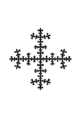
Figure 1. The Julia set of $\langle f_{1},f_{2}\rangle$, where $f_{1}(z)=z^{2}+2,f_{2}(z)=z^{2}-2$.

Proposition 9.2.

(See [42, 45]) Let $f_{1}$ be a semi-hyperbolic polynomial with $\deg(f_{1})\geq 2$ such that $J(f_{1})$ is connected. Let $K(f_{1})$ be the filled-in Julia set of $f_{1}$ and suppose that int$K(f_{1})$ is not empty. Let $b\in\mbox{{\em int}}K(f_{1})$ be a point. Let $d$ be a positive integer such that $d\geq 2.$ Suppose that $(\deg(f_{1}),d)\neq(2,2).$ Then, there exists a number $c>0$ such that for each $\lambda\in\{\lambda\in\mathbb{C}:0<|\lambda|<c\}$, setting $f_{\lambda}=(f_{\lambda,1},f_{\lambda,2})=(f_{1},\lambda(z-b)^{d}+b)$ and $G_{\lambda}:=\langle f_{1},f_{\lambda,2}\rangle$, we have that $G_{\lambda}$ is semi-hyperbolic and $f_{\lambda}$ satisfies the nice open set condition with an open set $U_{\lambda}$, $J(G_{\lambda})$ is porous, $\text{{\rm HD}}(J(G_{\lambda}))=h(f_{\lambda})<2$, and $P(G_{\lambda})\setminus\{\infty\}$ is bounded in $\mathbb{C}.$

Proof. We will follow the argument in [42, 45]. Conjugating $f_{1}$ by a Möbius transformation, we may assume that $b=0$ and the coefficient of the highest degree term of $f_{1}$ is equal to $1.$

Let $r>0$ be a number such that $\overline{B(0,r)}\subset\mbox{int}K(f_{1}).$ We set $d_{1}:=\deg(f_{1}).$ Let $\alpha>0$ be a number. Since $d\geq 2$ and $(d,d_{1})\neq(2,2)$, it is easy to see that $(\frac{r}{\alpha})^{\frac{1}{d}}>2\left(2(\frac{1}{\alpha})^{\frac{1}{d-1}}\right)^{\frac{1}{d_{1}}}$ if and only if

(9.1) $$\log\alpha<\frac{d(d-1)d_{1}}{d+d_{1}-d_{1}d}(\log 2-\frac{1}{d_{1}}\log\frac{1}{2}-\frac{1}{d}\log r).$$

We set

(9.2) $$c_{0}:=\exp\left(\frac{d(d-1)d_{1}}{d+d_{1}-d_{1}d}(\log 2-\frac{1}{d_{1}}\log\frac{1}{2}-\frac{1}{d}\log r)\right)\in(0,\infty).$$

Let $0<c<c_{0}$ be a small number and let $\lambda\in\mathbb{C}$ be a number with $0<|\lambda|<c.$ Put $f_{\lambda,2}(z)=\lambda z^{d}.$ Then, we obtain $K(f_{\lambda,2})=\{z\in\mathbb{C}\mid|z|\leq(\frac{1}{|\lambda|})^{\frac{1}{d-1}}\}$ and

$$f_{\lambda,2}^{-1}(\{z\in\mathbb{C}\mid|z|=r\})=\{z\in\mathbb{C}\mid|z|=(\frac{r}{|\lambda|})^{\frac{1}{d}}\}.$$

Let $D_{\lambda}:=\overline{B(0,2(\frac{1}{|\lambda|})^{\frac{1}{d-1}})}.$ Since $f_{1}(z)=z^{d_{1}}(1+o(1))\ (z\rightarrow\infty)$, it follows that if $c$ is small enough, then for any $\lambda\in\mathbb{C}$ with $0<|\lambda|<c$,

$$f_{1}^{-1}(D_{\lambda})\subset\left\{z\in\mathbb{C}\mid|z|\leq 2\left(2(\frac{1}{|\lambda|})^{\frac{1}{d-1}}\right)^{\frac{1}{d_{1}}}\right\}.$$

This implies that

(9.3) $$f_{1}^{-1}(D_{\lambda})\subset f_{\lambda,2}^{-1}(\{z\in\mathbb{C}\mid|z|<r\}).$$

Hence, setting $U_{\lambda}:=\mbox{int}K(f_{\lambda,2})\setminus K(f_{1})$, $f_{1}^{-1}(U_{\lambda})\cup f_{\lambda,2}^{-1}(U_{\lambda})\subset U_{\lambda}$ and $f_{1}^{-1}(U_{\lambda})\cap f_{\lambda,2}^{-1}(U_{\lambda})=\emptyset$. Furthermore, since $f_{1}$ is semi-hyperbolic, $\hat{\mathbb{C}}\setminus K(f_{1})$ is a John domain (see [6]). Hence, $U_{\lambda}$ satisfies (osc3). Therefore, $G_{\lambda}$ satisfies the nice open set condition with $U_{\lambda}.$ We have $J(G_{\lambda})\subset\overline{U_{\lambda}}\subset K(f_{\lambda,2})\setminus\mbox{int}K(f_{1}).$ In particular, int$K(f_{1})\cup(\hat{\mathbb{C}}\setminus K(f_{\lambda,2}))\subset F(G_{\lambda}).$ Furthermore, (9.3) implies that $f_{\lambda,2}(K(f_{1}))\subset\mbox{int}K(f_{1}).$ Thus, we have $P(G_{\lambda})\setminus\{\infty\}=\cup_{g\in G_{\lambda}^{\ast}}g(CV^{\ast}(f_{1})\cup CV^{\ast}(f_{\lambda,2}))\subset K(f_{1})$, where $CV^{\ast}(\cdot)$ denotes the set of all critical values in $\mathbb{C}.$ Hence, $P(G_{\lambda})\setminus\{\infty\}$ is bounded in $\mathbb{C}.$ Since $f_{1}$ is semi-hyperbolic, there exist an $N\in{\mathbb{N}}$ and a $\delta_{1}>0$ such that for each $x\in J(f_{1})$ and for each $n\in{\mathbb{N}}$, $\deg(f_{1}^{n}:V\rightarrow B(x,\delta_{1}))\leq N$ for each connected component $V$ of $f_{1}^{-n}(B(x,\delta_{1}).$ Moreover, $f_{\lambda,2}^{-1}(J(f_{1}))\cap K(h_{1})=\emptyset$ and so $f_{\lambda,2}^{-1}(J(f_{1}))\subset\hat{\mathbb{C}}\setminus P(G_{\lambda}).$ From these arguments, it follows that there exists a $0<\delta_{2}(<\delta_{1})$ such that for each $x\in J(f_{1})$ and each $g\in G_{\lambda}$, $\deg(g:V\rightarrow B(x,\delta_{2}))\leq N$ for each connected component $V$ of $g^{-1}(B(x,\delta_{2})).$ Since $P(G_{\lambda})\setminus\{\infty\}\subset K(f_{1})$ again, we obtain that there exists a $0<\delta_{3}(<\delta_{2})$ such that for each $x\in J(G_{\lambda})$ and each $g\in G_{\lambda}$, $\deg(g:V\rightarrow B(x,\delta_{3}))\leq N$ for each connected component $V$ of $g^{-1}(B(x,\delta_{3})).$ Thus, $G_{\lambda}$ is semi-hyperbolic. Since $J(G_{\lambda})\subset f_{1}^{-1}(\overline{U_{\lambda}})\cup f_{\lambda,2}^{-1}(\overline{U_{\lambda}})\subsetneqq\overline{U_{\lambda}}$, [39] implies that $J(G_{\lambda})$ is porous and $\text{{\rm HD}}(J(G_{\lambda}))<2.$ Moreover, by Theorem 1.11, we have $h(f_{\lambda})=\text{{\rm HD}}(J(G_{\lambda})).$ We are done. ∎

Figure 2. The Julia set of $\langle f_{1}^{2},f_{2}^{2}\rangle$, where $f_{1}(z)=z^{2}-1,f_{2}(z)=z^{2}/4$.