The radius and other fundamental parameters of the F9 V star $\mn@boldsymbol{\beta}$ Virginis

Abstract

We have used the Sydney University Stellar Interferometer (SUSI) to measure the angular diameter of the F9 V star $\beta$ Virginis. After correcting for limb darkening and combining with the revised Hipparcos parallax, we derive a radius of $1.703\pm 0.022$ $R_{\sun}$ (1.3 per cent). We have also calculated the bolometric flux from published measurements which, combined with the angular diameter, implies an effective temperature of $6059\pm 49$ K (0.8 per cent). We also derived the luminosity of $\beta$ Vir to be $L=3.51\pm 0.08\,L_{\sun}$ (2.1 per cent). Solar-like oscillations were measured in this star by Carrier et al. (2005) and using their value for the large frequency separation yields the mean stellar density with an uncertainty of about 2 per cent. Our constraints on the fundamental parameters of $\beta$ Vir will be important to test theoretical models of this star and its oscillations.

1 Introduction

Accurate measurements of fundamental stellar parameters – particularly radius, luminosity and mass – are essential for critically testing the current generation of stellar models. Some of these parameters can be constrained using well-established techniques such as spectrophotometry, parallax and optical interferometry. In the last decade, observing stellar oscillation frequencies (asteroseismology) has been shown to be a powerful tool to infer the internal structure of stars (e.g. Brown & Gilliland 1994). In particular, the mean stellar density can be estimated from the large frequency separation $\Delta\nu$ between consecutive radial overtones.

The links between asteroseismology and interferometry have been comprehensively reviewed by Cunha et al. (2007). Recently, the complementary roles played by these two techniques in the investigation of solar-type stars have been described by Creevey et al. (2007), who showed the mass of a single star can be determined to a precision (1-$\sigma$) of better than 2 per cent by combining a good radius measurement with the density inferred from the large separation. Indeed, this precision was almost obtained by North et al. (2007) when they constrained the mass of $\beta$ Hyi to a precision of 2.8 per cent using results from optical interferometry and asteroseismology (see also Kjeldsen et al. 2008). Moreover, North et al. (2007) further constrained the fundamental parameters of $\beta$ Hyi with values for the stellar radius, luminosity, effective temperature and surface gravity.

The star $\beta$ Virginis (HR 4540, HD 102870, HIP 57757) has spectral type F9 V (Morgan & Keenan, 1973) and is slightly metal-rich, with ${\rm[Fe/H]}=0.14$. It is bright ($V=3.60$) and has a well-determined parallax. Models by Eggenberger & Carrier (2006) using the Geneva evolution code, including rotation and atomic diffusion, indicate that the star has a mass of 1.2–1.3 M_☉ and is close to, or just past, the end of main-sequence core-hydrogen burning. Evidence for solar-like oscillations in $\beta$ Vir was reported by Martić et al. (2004), in the form of excess power at frequencies around 1.7 mHz. Subsequently, Carrier et al. (2005) confirmed the presence of oscillations and identified a series of regularly spaced modes with a large frequency separation of $\Delta\nu=72.1\,\mu$Hz.

In this paper we present the first interferometric measurement of the angular diameter of $\beta$ Vir (Section 2). We also calculate the bolometric flux of the star using data from the literature (Section 3). These, together with the parallax from Hipparcos and the density from asteroseismology, allow us to constrain the fundamental stellar parameters of $\beta$ Vir (effective temperature, radius, luminosity and mass; Section 4).

2 Angular Diameter

2.1 Interferometric Observations with SUSI

Measurements of the squared visibility $V^{2}$ (the normalised squared-modulus of the complex visibility) were made on a total of 12 nights using the Sydney University Stellar Interferometer (SUSI; Davis et al. 1999). We recorded interference fringes with the red-table beam-combination system using a filter with (nominal) centre wavelength 700 nm and full-width at half-maximum 80 nm. This beam-combination system has been described in Davis et al. (2007a) along with details of the standard SUSI observing, data reduction and calibration procedures.

The parameters of the calibrator stars are given in Table 1. There are no measured angular diameters for these stars, and the values given here were estimated from $(B-V)_{0}$ colours by interpolating measurements of similar stars with the Narrabri Stellar Intensity Interferometer (Hanbury Brown et al., 1974) and the Mark III Optical Interferometer (Mozurkewich et al., 2003). Corrections for limb-darkening were done using the results of Davis et al. (2000).

Table 1: Parameters of calibrator stars.

HR	Name	Spectral	V	UD Diameter	Separation
		Type		(mas)	from $\beta$ Vir
4368	$\phi$ Leo	A7IV	4.47	$0.58\pm 0.08$	10$\aas@@fstack{\circ}$08
4386	$\sigma$ Leo	B9V	4.04	$0.42\pm 0.06$	8$\aas@@fstack{\circ}$52
4515	$\xi$ Vir	A4V	4.84	$0.45\pm 0.06$	6$\aas@@fstack{\circ}$63

Table 2: Summary of observational data. The night of the observation is given in columns 1 and 2 as a calendar date and a mean MJD. The nominal and mean projected baseline in units of metres is given in columns 3 and 4, respectively. The weighted-mean squared visibility, associated error and number of observations during a night are given in the last three columns.

Date	MJD	Nominal	Mean Projected	Calibrators	${\bar{V}^{2}}$	${\bar{\sigma}}$	# $V^{2}$
		Baseline	Baseline
2007 February 14	54145.70	40	34.05	$\sigma$ Leo, $\phi$ Leo, $\xi$ Vir	0.684	0.030	3
2007 February 15	54146.66	60	51.28	$\sigma$ Leo, $\phi$ Leo	0.567	0.023	8
2007 March 09	54168.58	5	4.28	$\sigma$ Leo, $\phi$ Leo	1.006	0.037	3
2007 March 10	54169.58	60	51.35	$\sigma$ Leo, $\phi$ Leo	0.524	0.029	5
2007 March 11	54170.62	15	12.74	$\sigma$ Leo, $\phi$ Leo	0.893	0.018	5
2007 March 13	54172.63	5	4.26	$\sigma$ Leo, $\phi$ Leo	0.956	0.015	7
2007 March 14	54173.56	40	34.47	$\sigma$ Leo, $\phi$ Leo	0.706	0.015	6
2007 March 14	54173.68	15	13.25	$\sigma$ Leo, $\phi$ Leo	0.951	0.063	2
2007 March 15	54174.59	80	68.16	$\sigma$ Leo, $\phi$ Leo	0.264	0.010	8
2007 April 18	54108.47	5	4.31	$\sigma$ Leo, $\phi$ Leo	0.998	0.014	10
2007 April 20	54110.49	20	17.04	$\sigma$ Leo, $\phi$ Leo	0.957	0.032	4
2007 April 22	54112.49	80	68.01	$\sigma$ Leo, $\phi$ Leo	0.339	0.014	6
2007 May 27	54147.39	80	68.32	$\sigma$ Leo, $\phi$ Leo	0.304	0.009	10

The journal of observations is given in Table 2. We obtained a total of 77 estimations of $V^{2}$. It should be noted that, for consistency, the uncertainties in the angular diameters of the calibrating stars were included in the $V^{2}$ uncertainty calculation, even though they have a negligibly small effect when compared to the measurement uncertainty.

2.2 Analysis of Visibilities

In the simplest case, the brightness distribution of a star can be modeled as a disc of uniform irradiance with angular diameter $\theta_{\rm UD}$. The theoretical response of a two-aperture interferometer to such a model is given by

$$|V|^{2}=\left|\frac{2J_{1}(\pi B\theta_{\rm UD}/\lambda)}{\pi B\theta_{\rm UD}/\lambda}\right|^{2},$$ (1)

where $B$ is the projected baseline, $\lambda$ is the observing wavelength and $J_{1}$ is a first order Bessel function. However, real stars are limb-darkened and corrections are needed to find the ‘true’ angular diameter. These corrections can be found in Davis, Tango & Booth (2000) and are small for stars that have a compact atmosphere.

To account for any systematic effects arising from the slightly differing spectral types of $\beta$ Vir and the calibrators, the presence of a close companion, or other causes, an additional parameter, $A$, is included in the uniform disc model. Equation (1) becomes

$$|V|^{2}=\left|A\frac{2J_{1}(\pi B\theta_{\rm{UD}}/\lambda)}{\pi B\theta_{\rm{UD}}/\lambda}\right|^{2}.$$ (2)

The interferometer response given in equation (2) is, strictly speaking, only valid for monochromatic observations. Tango & Davis (2002) have analysed the effect of a wide observing bandpass on interferometric angular diameters and found it to be insignificant provided the interferometer’s coherent field-of-view is larger than the angular extent of the source. The coherent field-of-view of SUSI during observations was found to be greater than 5.8 mas, hence greater than the extent of $\beta$ Vir (see below). Therefore, bandwidth smearing can be considered negligible. However, SUSI’s effective wavelength when observing an F9 star is approximately $696.4\pm 2.0$ nm (Davis et al., 2007a). The fit to equation (2) was completed with this effective wavelength.

An implementation of the Levenberg-Marquardt method was used to fit equation (2) to all measures of $V^{2}$ to estimate $\theta_{\rm UD}$ and $A$. The diagonal elements of the covariance matrix (which are calculated as part of the $\chi^{2}$ minimisation) were used to derive formal uncertainties in the parameter estimation. We used Markov chain Monte Carlo (MCMC) simulations to verify the formal uncertainties because equation (2) is non-linear and the squared visibility measurement errors (derived by the SUSI reduction pipeline) may not strictly conform to a normal distribution. A MCMC simulation, implemented with a Metropolis-Hastings algorithm, involves a likelihood-based random walk in parameter space whereby the full marginal posterior probability density function is estimated for each parameter (see Gregory 2005 for an introduction to MCMC). An advantage of this method is that prior information (and the effect on parameter uncertainties) can be included in the simulation. In the case of $\beta$ Vir, the effect of the observing wavelength uncertainty was included in the simulation by the adoption of an appropriate likelihood function (see below).

The reduced $\chi^{2}$ of the original fit was 2.08, implying that the squared-visibility measurement uncertainties were underestimated. We have therefore scaled the measurement uncertainties by $\sqrt{2.08}$ to obtain a reduced $\chi^{2}$ of unity. The formal uncertainties were verified with a series of MCMC simulations, each comprising $10^{6}$ iterations. For the effective wavelength we adopted a Gaussian likelihood function with mean 696 nm and standard deviation 2 nm. The probability density functions produced Gaussian distributions with standard deviation of similar values to the formal uncertainties. We therefore obtain (with the associated $1\sigma$ formal uncertainty) $\theta_{\rm UD}=1.386\pm 0.017$ mas and $A=0.985\pm 0.006$. The data are shown in Fig. 1 with the fitted uniform-disc model overlaid.

Figure 1: Nightly weighted-mean $V^{2}$ measures with the fitted uniform disc model overlaid. Inset: all $V^{2}$ measures at the (nominal) 80 m SUSI baseline.

The fitted value of $A$ differs slightly from unity, indicating there is either a close companion or some instrumental effect causing a small reduction in the $V^{2}$ intercept. While $\beta$ Vir does have known optical companions, these stars are too distant and too faint to affect the SUSI observations. Furthermore, $\beta$ Vir appears in planet search programs (see for example Wittenmyer et al. 2006) and there is only a very limited parameter space where a further companion could reside without having already been detected. We also cannot explain the value of $A$ in terms of a systematic reduction of $V^{2}$ due to the slightly differing spectral types of target and calibrator stars. We believe it is more likely that the observations were affected by a small unknown systematic error or a binary companion of unusual characteristics, than that they were subject to unlucky large random errors. Therefore, we retain the original uniform disc angular diameter, $\theta_{\rm UD}=1.386\pm 0.017$ mas, fitted with $A$ as a free parameter.

The correction for the effects of limb-darkening was determined to be $\theta_{\rm LD}=1.046\theta_{\rm UD}$, using Davis et al. (2000) and the following parameters: $T_{\rm eff}=6059$ K, $\log g=4.12$ and ${\rm[Fe/H]}=0.14$. With the exception of [Fe/H], these values are the result of an iterative procedure whereby initial values were refined by the subsequent determination of fundamental parameters in Section 4. The starting values for $T_{\rm eff}$ and $\log g$, and the fixed value for [Fe/H], were the mean values from those found in the literature, and are given in Table 3. The refinement of $T_{\rm eff}$ and $\log g$ only caused a small change in the fifth significant figure of the limb-darkening correction, for which we estimate an uncertainty 0.002. Therefore the limb-darkened diameter is $\theta_{\rm LD}=1.450\pm 0.018$ mas and carries the caveat that we are assuming that the Kurucz models, upon which Davis et al. (2000) based their work, are accurate for this star.

Table 3: Literature values for parameters of $\beta$ Vir.

Source	$T_{\rm eff}$ (K)	Method#	$\log g$	[Fe/H]
1	$6150\pm 100$	a	$4.2\pm 0.1$	0.10
2	$6190\pm 80$	b	$4.20$	0.13
3	$6176$	b	$4.14$	0.13
4	$6127\pm 55$	c	-	-
5	$6124\pm 31$	c	-	-
6	$6124^{\dagger}$		$4.24^{\dagger}$	$0.19^{\dagger}$
7	$6068\pm 70$	b	$4.09\pm 0.1$	$0.13\pm 0.1$
8	$6140$	d	$4.09\pm 0.08$	0.15
9	$6055\pm 48$	e	-	-
10	$6124$	f	-	$0.13\pm 0.10$
11	$6076\pm 119$	b	$4.142$	0.13
Mean	6123		$4.16$	0.14

Source references: (1) Thévenin, Vauclair & Vauclair (1986); (2) Balachandran (1990); (3) Edvardsson et al. (1993); (4) di Benedetto (1998); (5) Blackwell & Lynas-Gray (1998); (6) Malagnini et al. (2000); (7) Chen et al. (2001); (8) Gray et al. (2001); (9) Kovtyukh et al. (2003); (10) Morel & Micela (2004); (11) Allende Prieto et al. (2004).

^†: mean of listed values from elsewhere, many identical;

^#: method used for $T_{\rm{eff}}$ determination: (a) Fit to H$\gamma$ profile; (b) From $b$ and ($b-y$) calibration; (c) IRFM method; (d) Fits of model spectra to spectra and $uby$; (e) From line depth ratios; (f) From iron line excitation and ionization equilibrium.

3 Bolometric Flux

We have determined the bolometric flux, $f$, based on flux-calibrated photometry and spectrophotometry from the literature in combination with MARCS model stellar atmospheres (Gustafsson et al., 2003). It has been determined by summing the integrated fluxes over four spectral ranges, namely $<0.33\,\mu$m, 0.33–0.86 $\mu$m, 0.86–2.2 $\mu$m and 2.2–20 $\mu$m. The flux beyond 20 $\mu$m is $<0.01$ per cent for a 6150 K black body and will be similar for the stellar flux distribution and can be ignored. It is noted that the ($B-V$) and ($U-B$) colours of $\beta$ Vir are consistent with those of an unreddened star of its spectral classification.

Kiehling (1987) has published spectrophotometry of $\beta$ Vir for the wavelength range 325–865 nm. The observations were made at equal intervals of 1 nm with a resolution of 1 nm. The published spectral energy distribution is averaged over bandpasses 5 nm wide and is tabulated every 5 nm, based on the spectrophotometric calibration of Vega by Hayes (1985). This has been converted to a flux distribution using a value for the flux from Vega at 550.0 nm of 3.56$\times$10^-11 Wm^-2nm^-1 (Megessier, 1995). In the case of $\delta$ CMa (Davis et al., 2007b), Kiehling’s spectrophotometry was compared with that of Davis & Webb (1974) and the calibrated flux distributions were found to be in excellent agreement, with an RMS difference computed from the wavelengths in common of $<$ 1.1 per cent and with no systematic differences over the wavelength range in common (330–808 nm). The flux distribution in the MILES library of empirical spectra (Sánchez-Blázquez et al., 2006) for $\beta$ Vir has also been considered and has been flux-calibrated in the same way as the Kiehling data. The wavelength coverage of the MILES flux distribution is 355–740 nm, less than the Kiehling range of 325–865 nm. It is tabulated at 0.9 nm intervals with a resolution of 0.23 nm, compared with the data by Kiehling, which were averaged and tabulated over 5 nm intervals. The two distributions are in excellent agreement except for two apparently discrepant points in the Kiehling distribution at 760 nm and 765 nm. The two flux distributions were integrated for the common wavelength range of 355–740 nm, omitting the discrepant points, and the integrated fluxes agree to within 1 per cent. The Kiehling flux distribution covers a greater wavelength range and extends to the ultraviolet data at the short wavelength end and, for these reasons, it has been used to determine the integrated visual flux.

The uncertainty in the integrated flux has been estimated by combining the uncertainty in the Megessier (1995) flux calibration of 0.7 per cent, the uncertainty in the Vega calibration by Hayes (1985) of 1.5 per cent and the uncertainty in the relative flux distribution of Kiehling (1987), which is estimated to be $\sim$1.5 per cent. This latter figure is based on the previous experience with $\delta$ CMa and the good agreement between the Kiehling and MILES flux distributions for $\beta$ Vir. The resultant uncertainty is $\pm$2.2 per cent and the integrated Kiehling flux for the wavelength range 0.33–0.86 $\mu$m is $(5.73\pm 0.13)\times 10^{-10}\,{\rm Wm}^{-2}$.

There are four flux values for the ultraviolet from the TD1 satellite (Thompson et al., 1978) at 156.5, 196.5, 236.5 and 274.0 nm and these have been downloaded from SIMBAD. They have been plotted with the Kiehling (1987) calibrated fluxes at 325 and 330 nm and a smooth curve drawn through the six flux points. The flux shortward of 330 nm is only a small fraction of the total flux ($<$4 per cent), justifying this simple approach. The area under the curve shortward of 330 nm has been integrated to give the ultraviolet flux equal to $(3.5\pm 0.2)\times 10^{-11}\,{\rm Wm}^{-2}$ where the uncertainty is conservatively based on the published uncertainties in the ultraviolet fluxes.

There are few infrared measurements for $\beta$ Vir and it was necessary to interpolate and extrapolate them with the aid of a MARCS model stellar atmosphere (Gustafsson et al., 2003). The calibrated observational photometric fluxes are listed in Table 4, together with their sources and the references used for their calibration, and the fluxes are shown in Fig. 2. Initially the flux distributions of MARCS model atmospheres for 6000 K and 6250 K, both for $\log{g}=4.0$, were scaled to fit the observational data in the wavelength range 0.6–2.2 $\mu$m. The observational data included the Kiehling fluxes from 0.6–0.865 $\mu$m and the fluxes for the $RIJHK$ photometric bands listed in Table 4. The 6000 K model gave a good fit but the 6250 K model clearly did not. The scaled fluxes for the 6000 K model were integrated in two ranges, 0.86–2.2 $\mu$m and 2.2–20 $\mu$m. The resulting integrated fluxes were added to the fluxes for $<$0.33 $\mu$m and 0.33–0.86 $\mu$m determined above and, in combination with the limb-darkened angular diameter, gave an effective temperature of $\sim$6050 K.

Table 4: Calibrated photometric IR fluxes for $\beta$ Vir

Band	$\lambda_{\rm{eff}}$	Flux	Source	Calibration
	($\mu$m)	($10^{-12}{\rm Wm}^{-2}\mu{\rm m}^{-1}$)
$R$	0.641	105.8	1	a
$I$	0.798	71.6	1	a
$R$	0.70	99.0	2	b
$I$	0.90	61.0	2	b
$J$	1.25	28.0	2	c
$K$	2.20	4.8	2	c
$J$	1.2790	27.05	3	d
$H$	1.6483	12.54	3	d
$K$	2.1869	5.01	3	d
12$\mu$m	12	0.0104	4	e

Source references: (1) Cousins (1980); (2) Johnson et al. (1966); (3) Alonso et al. (1994); (4) IRAS Team (1988).

Calibration references: (a) Bessell et al. (1998); (b) Johnson (1966); (c) Megessier (1995); (d) Alonso et al. (1994); (e) IRAS Team (1988) reduced by 4.1 per cent (Cohen et al., 1996).

The fluxes for an effective temperature of 6050 K were interpolated from the 6000 K and 6250 K models and the fitting procedure repeated. The models have fluxes tabulated at intervals of 0.005 per cent in wavelength, which results in very large plot files. For diagrammatic purposes the fitting was therefore also carried out with different flux averages—0.025, 0.05 and 1.0 per cent intervals in wavelength. No significant difference was found in either the scaling factor for a fit or in the integrated fluxes for the different flux averages. The fit for the interpolated fluxes for 6050 K averaged over 0.025 per cent wavelength intervals is shown in Fig. 2. Uncertainties in the integrated fluxes have been derived by combining the estimated uncertainty in the fit to the observational data with the uncertainty in the observational data and in particular that in the Kiehling data involved in the fit.

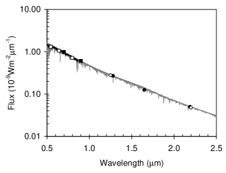
Figure 2: The flux distribution for $\beta$ Vir for the wavelength range 0.5–2.5 $\mu$m, with data from Table 4. The symbols have been plotted oversize for clarity. Key: small filled circles - Kiehling (1987); open squares - Cousins (1980) $VRI$ photometry; filled squares - Johnson et al. (1966) $RI$ photometry; open circles - Johnson et al. (1966) $JK$ photometry; filled circles - Alonso et al. (1994) $JHK$ photometry; grey line - fluxes for the fitted MARCS model atmosphere averaged over 0.025 per cent wavelength intervals.

The integrated fluxes for the fitted 6050 K flux distribution are listed in Table 5 for the four wavelength bands considered. The uncertainties have been derived by combining the estimated uncertainty in the fit to the observational data with the uncertainty in the observational data and in particular that in the Kiehling data involved in the fit.

Figure 3 shows an assembly of the observational flux data with the interpolated flux curve for a 6050 K model atmosphere fitted to the observational data as shown in Fig. 2. Figure 3 includes mid-infrared photometry from Spitzer by Trilling et al. (2008) and we note that the data appear to rule out their suggestion of a possible excess from a debris disk. The 12 $\mu$m IRAS Point Source flux does lie above the model curve but drawing a smooth curve from the flux for the $K$ band through the IRAS point and integrating it over the range 2.2–20 $\mu$m shows that it has negligible effect on the bolometric flux ($<$0.04 per cent) or effective temperature ($<$1 K).

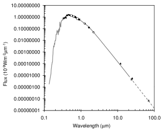
Figure 3: The flux distribution for $\beta$ Vir from the ultraviolet to the mid-infrared. Symbols have the same meanings as Fig. 2, with the addition of: filled triangles - IRAS Point Source Fluxes; and open triangles - Spitzer fluxes (Trilling et al., 2008). The dashed grey line is an extension of the MARCS model beyond 20 $\mu$m using a slope of $\lambda^{-4}$.

The resulting bolometric flux is $(9.44\pm 0.20)\times 10^{-10}\,{\rm Wm}^{-2}$, where the estimated uncertainty takes into account the fact that the uncertainties in the integrated fluxes for the wavelength ranges 0.33–0.86 $\mu$m, 0.86–2.2 $\mu$m and 2.2–20 $\mu$m are only partially independent. Our value is consistent with two previous determinations, namely $9.408\times 10^{-10}$ Wm^-2 by Alonso et al. (1995) and $9.59\times 10^{-10}$ Wm^-2 by Blackwell & Lynas-Gray (1998).

Table 5: Integrated fluxes for $\beta$ Vir in each spectral band and the resulting bolometric flux ($f$).

Wavelength	Flux
Range	(10-10Wm-2)
($\mu$m)
0–0.33	$0.35\pm 0.02$
0.33–0.86	$5.73\pm 0.13$
0.86–2.2	$2.97\pm 0.09$
2.2–20	$0.39\pm 0.02$
$>$20	negligible
$f$	$9.44\pm 0.20$

Table 6: Physical parameters of $\beta$ Vir. Estimates for density, mass and $\log g$ are given for two different values of $\Delta\nu$ (see text).

Parameter	Value	Uncertainty (per cent)
$\theta_{\rm LD}$ (mas)	$1.450\pm 0.018$	1.2
$f$ ($10^{-10}$ Wm-2)	$9.44\pm 0.20$	2.1
$\pi_{\rm p}$ (mas)	$91.50\pm 0.22$a	0.24
$R$ (R☉)	$1.703\pm 0.022$	1.3
$T_{\rm eff}$ (K)	$6059\pm 49$	0.8
$L$ (L☉)	$3.51\pm 0.08$	2.1
$\Delta\nu$ ($\mu$Hz)	$72.07\pm 0.10$	0.14
$\bar{\rho}$ (g cm-3)	$0.4028\pm 0.0081$	2.0
$M$ (M☉)	$1.413\pm 0.061$	4.3
$\log(g/{\rm cm\,s}^{-2})$	$4.125\pm 0.010$	2.4 (in $g$)
$\Delta\nu$ ($\mu$Hz)	$70.5$
$\bar{\rho}$ (g cm-3)	$0.3851\pm 0.0077$	2.0
$M$ (M☉)	$1.351\pm 0.058$	4.3
$\log(g/{\rm cm\,s}^{-2})$	$4.106\pm 0.010$	2.4 (in $g$)

^a van Leeuwen (2007)

4 Stellar Parameters

The observable quantities, limb-darkened angular diameter ($\theta_{\mathrm{LD}}$), bolometric flux ($f$) received from the star, parallax ($\pi_{\rm p}$) and large separation ($\Delta\nu$) combine to produce experimental constraints on the stellar radius ($R$), effective temperature ($T_{\rm eff}$), luminosity ($L$), mean density ($\bar{\rho}$), mass ($M$) and surface gravity ($\log g$). Values for these observable quantities are given in Table 6, along with the stellar parameters that are calculated in the remainder of this Section.

4.1 Radius

The stellar radius can be determined using our limb-darkened angular diameter and the Hipparcos parallax,

$$R=\theta_{\mathrm{LD}}\frac{C}{2\pi_{\rm p}},$$ (3)

where $C$ is the conversion from parsecs to metres, $\theta_{\mathrm{LD}}$ is in radians and $\pi_{\rm p}$ is in arcsec. Note that the revised Hipparcos parallax of $91.50\pm 0.22$ mas (van Leeuwen, 2007) has a substantially smaller uncertainty than the original value of $91.74\pm 0.77$ (Perryman et al., 1997). We obtain a stellar radius for $\beta$ Vir of $1.703\pm 0.022$ $R_{\sun}$. This is in excellent agreement with $1.706\pm 0.037$ R_☉ produced from surface brightness relations and the Hipparcos parallax by Thévenin et al. (2006), but is more precise and is based on a direct measurement.

4.2 Effective Temperature

The combination of the stellar bolometric flux and angular diameter yields an empirical effective temperature:

$$T_{\rm eff}=\left(\frac{4f}{\sigma\theta_{\mathrm{LD}}^{2}}\right)^{1/4},$$ (4)

where $\sigma$ is the Stefan-Boltzmann constant. Combining the new value for the bolometric flux (Section 3) with the limb-darkened angular diameter (Section 2) gives the effective temperature for $\beta$ Vir as $6059\pm 49$ K.

The new value for the effective temperature can be compared with the previous estimates listed in Table 3. There is excellent agreement with the line-depth ratio determination by Kovtyukh et al. (2003) and the determinations by Chen et al. (2001) and Allende Prieto et al. (2004) from the Strömgren photometry using the calibrations by Alonso et al. (1996) and Allende Prieto & Lambert (1999). The methods are completely independent, with only the new value presented here being based on a direct measurement of the angular diameter of the star.

The values for the bolometric flux of $9.408\times 10^{-10}\,{\rm Wm}^{-2}$ by Alonso et al. (1995) and $9.59\times 10^{-10}\,{\rm Wm}^{-2}$ by Blackwell & Lynas-Gray (1998) led those authors to effective temperatures of 6088 K and 6124 K respectively. However, if their bolometric fluxes are combined with our value for the limb-darkened angular diameter they give effective temperatures of 6054 K and 6083 K respectively, both of which are consistent with the value for the effective temperature presented here.

4.3 Luminosity

The luminosity of a star can be calculated via

$$L=4\pi f\frac{C^{2}}{\pi_{\rm p}^{2}},$$ (5)

where $C$ is the conversion from parsecs to metres and $\pi_{\mathrm{p}}$ is in arcsec. Substituting our value for $f$ gives $L=(1.349\pm 0.029)\times 10^{26}$ W. Following the work of Bahcall et al. (2001), we have adopted L${}_{\sun}=(3.842\pm 0.015)\times 10^{26}$ W and so get $L=3.51\pm 0.08\,L_{\sun}$.

A recent determination of $\beta$ Vir’s luminosity by Eggenberger & Carrier (2006), based on applying a bolometric correction to the absolute visual magnitude, gave $3.51\pm 0.10$ L_☉, which agrees with our value.

4.4 Mean Density from Asteroseismology

Carrier et al. (2005) collected high-precision velocity measurements of $\beta$ Vir over eleven nights with the CORALIE spectrograph. The Fourier spectrum showed a clear power excess in a broad frequency range centred at 1.5 mHz, confirming the presence of solar-like oscillations first reported by Martić et al. (2004). Carrier et al. found that the autocorrelation of their power spectrum showed peaks at 70.5, 72 and 74 $\mu$Hz, and they identified the second of these as the most likely value for the large frequency separation. After extracting oscillation frequencies and fitting to the asymptotic relation (Tassoul, 1980), they reported a value for the large separation of $72.07\pm 0.10\,\mbox{$\mu$Hz}$.

To a good approximation, the mean stellar density can be calculated from the observed large frequency separation (e.g. Ulrich, 1986):

$$\frac{\Delta\nu}{\Delta\nu_{\sun}}=\sqrt{\frac{\bar{\rho}}{\bar{\rho}_{\sun}}}.$$ (6)

Using the large separation for $\beta$ Vir reported by Carrier et al. (2005), and adopting solar values of $\bar{\rho}_{\sun}=1.408$ g cm^-3 and $\Delta\nu_{\sun}=134.8$ $\mu$Hz (Kjeldsen et al., 2008), we obtain $\bar{\rho}=0.4028$ g cm^-3.

It is important to note that equation (6) is an approximation. In particular, $\Delta\nu$ in a given star varies systematically with both frequency and with the angular degree of the modes. A more sophisticated approach involves comparing the observed oscillation frequencies with those calculated from an appropriate stellar model (this was done for $\beta$ Vir by Eggenberger & Carrier 2006). Unfortunately, due to the difficulty in modelling convection in the surface layers of stars, model calculations do not exactly reproduce observed oscillation frequencies, even for the Sun (Christensen-Dalsgaard et al., 1988; Dziembowski et al., 1988; Rosenthal et al., 1999; Li et al., 2002). This discrepancy increases with frequency, which means that the large separation is incorrectly predicted by the model calculations. For example, as discussed by Kjeldsen et al. (2008), the best models of the Sun have a large separation that is about 1 $\mu$Hz greater than the observed value.

To address this problem, Kjeldsen et al. (2008) have proposed an empirical method for correcting the frequencies of stellar models. They applied this method to the stars $\alpha$ Cen A, $\alpha$ Cen B and $\beta$ Hyi and obtained very accurate estimates of the mean stellar densities (better than 0.5 per cent). The same approach was used by Teixeira et al. (2009) to measure the density of $\tau$ Cet with similar precision.

We have attempted to apply this method to $\beta$ Vir, using the oscillation frequencies published by Carrier et al. (2005). We computed theoretical models using the Aarhus stellar evolution code (ASTEC, Christensen-Dalsgaard 2008a), and oscillation frequencies using the Aarhus adiabatic oscillation package (ADIPLS, Christensen-Dalsgaard 2008b). We followed the method described by Kjeldsen et al. (2008), which involves fitting both $\Delta\nu$ and the absolute frequencies of the radial modes (i.e., those having degree $l=0$). The method makes use of the fact that the frequency offset between observations and models should tend to zero with decreasing frequency. However, we were not able to achieve a fit with models whose fundamental parameters (luminosity and radius) agreed with the measured values. In other words, the frequencies of the radial modes listed by Carrier et al. (2005) do not appear to be consistent with models. Indeed, for $\beta$ Vir Eggenberger & Carrier (2006) remarked on an offset of more than 20 $\mu$Hz between observed and calculated frequencies, which they noted to be substantially larger than the corresponding offset for the Sun. Note that our conclusion that the published frequencies are inconsistent with models is not sensitive to the input physics of the evolutionary models. Kjeldsen et al. (2008) demonstrated that their fitting process works for models published by different authors using a range of model codes.

Two effects could have introduced a systematic offset to the observed frequencies. Firstly, an offset of $\pm 11.6\,\mbox{$\mu$Hz}$ could occur because of the cycle-per-day aliases in the power spectrum, which are strong in single-site observations such as those obtained for $\beta$ Vir. Indeed, many of the frequencies listed by Carrier et al. (2005, their Table 2) were shifted by 11.6 $\mu$Hz in one direction or the other in order to give a good fit to the p-mode spectrum. This includes the highest peak in the power spectrum, from which 11.6 $\mu$Hz was subtracted.

A second possibility is that the modes were misidentified, so that modes of odd and even degree were interchanged. That is, modes identified as having degree $l=0$ actually have degree $l=1$, and vice versa. Such a misidentification is plausible and, in the context of the method of Kjeldsen et al., would be equivalent to subtracting an offset of ${\textstyle\frac{1}{2}}\mbox{$\Delta\nu$}\approx 36\,\mbox{$\mu$Hz}$ from the frequencies of all modes.

We found that neither of the above corrections was able to give a consistent result, but we did find a good agreement between models and observations if we applied both together. That is, adding 11.6 $\mu$Hz and subtracting $36\,\mbox{$\mu$Hz}$ from the frequencies identified as radial modes gave a sensible result. However, if this scenario is correct then the whole mode identification process would be called into question, and it would be risky to rely on the tabulated frequencies to establish a precise density.

Until more oscillation data become available, we therefore fall back on the density that we determined from equation (6). Looking at the results for other stars (Kjeldsen et al., 2008; Teixeira et al., 2009), we estimate that this relation gives the mean density with an uncertainty of about 2 per cent. We have therefore adopted this value for the uncertainty in the density, as shown in Table 6.

4.5 Mass and Evolutionary State

Combining our radius measurement with the mean density inferred from asteroseismology, we calculate the mass to be $1.413\pm 0.061$ M_☉. This is slightly higher than previous estimates based on fitting models in the H-R diagram: $1.36\pm 0.09$ M_☉ (Allende Prieto & Lambert, 1999), $1.32$ M_☉ (Chen et al., 2001) and $1.34\pm 0.10$ M_☉ (Lambert & Reddy, 2004). The difference is not statistically significant, but we should point out that adopting a value of $\mbox{$\Delta\nu$}=70.5\,\mbox{$\mu$Hz}$, which is another of the three peaks in the autocorrelation of the observed power spectrum identified by Carrier et al. (2005), gives a mass of $1.35\,M_{\sun}$. This value, which is also shown in Table 6, is in better agreement with the location of the star in the H-R diagram. The models by Eggenberger & Carrier (2006) suggest that $\beta$ Vir either has a mass of $\sim$1.3 M_☉ and is towards the end of its main-sequence lifetime, or else it has mass of $\sim$1.2 M_☉ and is in the post main-sequence phase. Assuming that one of 70.5 or 72.1 $\mu$Hz is the correct large spacing, then the post main-sequence model appears to be excluded, indicating that $\beta$ Vir is still on the main sequence. Clearly, establishing the age of the star is also affected by the uncertainy in the mass. A more precise determination of its mass and evolutionary state will require further observations of its oscillations, preferably from multiple sites.

Substituting the stellar mass with the mean density and volume, the standard surface gravity relation becomes

$$g=\frac{4}{3}G\pi\bar{\rho}R,$$ (7)

where $G$ is the universal constant of gravitation. In Table 6 we show $\log g$ for the two values of $\Delta\nu$. Both determinations are consistent with the published values (see Table 3), which is not surprising given that spectroscopic determinations of $\log g$ are not very precise.

5 Conclusion

We have presented the first angular diameter measurement of the F9 V star $\beta$ Vir. In combination with the revised values for the bolometric flux and parallax, this angular diameter has experimentally constrained the stellar radius and effective temperature. The radius measurement, combined with the mean density determined from asteroseismology, allows an estimate of $\beta$ Vir’s mass and surface gravity.

The constraints on $R$, $T_{\rm eff}$, $M$, $\log g$ and $L$ that we present will be invaluable in the future to further test theoretical models of $\beta$ Vir and its oscillations. As stressed by Brown & Gilliland (1994), for example, oscillation frequencies are of most importance for testing evolution theories when the other fundamental stellar properties are well-constrained.

References

- Allende Prieto & Lambert (1999) Allende Prieto C., Lambert D. L., 1999, A&A, 352, 555
- Allende Prieto et al. (2004) Allende Prieto C., Barklem P. S., Lambert D. L., Cunha K., 2004, A&A, 420, 183
- Alonso et al. (1994) Alonso A., Arribas S., Martinez-Roger C., 1994, A&A, 107, 365
- Alonso et al. (1995) Alonso A., Arribas S., Martinez-Roger C., 1995, A&A, 297, 197
- Alonso et al. (1996) Alonso A., Arribas S., Martinez-Roger C., 1996, A&A, 313, 873
- Bahcall et al. (2001) Bahcall J. N., Pinsonneault M. H., Basu S., 2001, ApJ, 555, 990
- Balachandran (1990) Balachandran S., 1990, ApJ, 354, 310
- Bessell et al. (1998) Bessell M. S., Castelli F., Plez B., 1998, A&A, 333, 231
- Blackwell & Lynas-Gray (1998) Blackwell D. E., Lynas-Gray A. E., 1998, A&AS, 129, 505
- Brown & Gilliland (1994) Brown T. M., Gilliland R. L., 1994, ARA&A, 32, 37
- Carrier et al. (2005) Carrier F., Eggenberger P., D’Alessandro A., Weber L., 2005, NewA, 10, 315
- Chen et al. (2001) Chen Y. Q., Nissen P. E., Benoni T., Zhao G., 2001, A&A, 371, 943
- Christensen-Dalsgaard (2008a) Christensen-Dalsgaard J., 2008a, Ap&SS, 316, 13
- Christensen-Dalsgaard (2008b) Christensen-Dalsgaard J., 2008b, Ap&SS, 316, 113
- Christensen-Dalsgaard et al. (1988) Christensen-Dalsgaard J., Däppen W., Lebreton Y., 1988, Nat, 336, 634
- Cohen et al. (1996) Cohen M., Witteborn F. C., Carbon D. F., Davies J. K., Wooden D. H., Bregman J. D., 1996, AJ, 112, 2274
- Cousins (1980) Cousins A. W. J., 1980, SAAO Circ., 1, 234
- Creevey et al. (2007) Creevey O. L., Monteiro M. J. P. F. G., Metcalfe T. S., et al., 2007, ApJ, 659, 616
- Cunha et al. (2007) Cunha M. S., Aerts C., Christensen-Dalsgaard J., et al., 2007, A&AR, 14, 217
- Davis & Webb (1974) Davis J., Webb R. J., 1974, MNRAS, 168, 163
- Davis et al. (1999) Davis J., Tango W. J., Booth A. J., ten Brummelaar T. A., Minard R. A., Owens S. M., 1999, MNRAS, 303, 773
- Davis et al. (2000) Davis J., Tango W. J., Booth A. J., 2000, MNRAS, 318, 387
- Davis et al. (2007a) Davis J., Ireland M. J., Chow J., Jacob A. P., Lucas R. E., North J. R., O’Byrne J. W., Owens S. M., Robertson J. G., Seneta E. B., Tango W. J., Tuthill P. G., 2007a, PASA, 24, 138
- Davis et al. (2007b) Davis J., Booth A. J., Ireland M. J., Jacob A. P., North J. R., Owens S. M., Robertson J. G., Tango W. J., Tuthill P. G., 2007b, PASA, 24, 151
- di Benedetto (1998) di Benedetto G. P., 1998, A&A, 339, 858
- Dziembowski et al. (1988) Dziembowski W. A., Paternó L., Ventura R., 1988, A&A, 200, 213
- Edvardsson et al. (1993) Edvardsson B., Andersen J., Gustafsson B., Lambert D. L., Nissen P. E., Tomkin J., 1993, A&A, 275, 101
- Eggenberger & Carrier (2006) Eggenberger P., Carrier F., 2006, A&A, 449, 293
- Gray et al. (2001) Gray R. O., Graham P. W., Hoyt S. R., 2001, AJ, 121, 2159
- Gregory (2005) Gregory P. C., 2005, Bayesian Logical Data Analysis for the Physical Sciences. Cambridge University Press
- Gustafsson et al. (2003) Gustafsson B., Edvardsson B., Eriksson K., Mizuno-Wiedner M., Jørgensen U. G., Plez B., 2003, in Hubeny I., Mihalas D., Werner K., eds, Stellar Atmosphere Modeling Vol. 288 of ASP Conf. Series, A Grid of Model Atmospheres for Cool Stars. p. 331
- Hanbury Brown et al. (1974) Hanbury Brown R., Davis J., Allen L. R., 1974, MNRAS, 167, 121
- Hayes (1985) Hayes D. S., 1985, in Hayes D. S., Pasinetti L. E., Philip A. G. D., eds, Calibration of Fundamental Stellar Quantities Vol. 111 of IAU Symp., Stellar absolute fluxes and energy distributions from 0.32 to 4.0 microns. p. 225
- IRAS Team (1988) IRAS Team 1988, The IRAS Point Source Catalog, version 2.0. NASA RP–1190
- Johnson (1966) Johnson H. L., 1966, ARA&A, 4, 193
- Johnson et al. (1966) Johnson H. L., Iriarte B., Mitchell R. I., Wisniewskj W. Z., 1966, Comm. Lunar and Planetary Lab., 4, 99
- Kiehling (1987) Kiehling R., 1987, A&AS, 69, 465
- Kjeldsen et al. (2008) Kjeldsen H., Bedding T. R., Christensen-Dalsgaard J., 2008, ApJ, 683, L175
- Kovtyukh et al. (2003) Kovtyukh V. V., Soubiran C., Belik S. I., Gorlova N. I., 2003, A&A, 411, 559
- Lambert & Reddy (2004) Lambert D. L., Reddy B. E., 2004, MNRAS, 349, 757
- Li et al. (2002) Li L. H., Robinson F. J., Demarque P., Sofia S., Guenther D. B., 2002, ApJ, 567, 1192
- Malagnini et al. (2000) Malagnini M. L., Morossi C., Buzzoni A., Chavez M., 2000, PASP, 112, 1455
- Martić et al. (2004) Martić M., Lebrun J.-C., Appourchaux T., Korzennik S. G., 2004, A&A, 418, 295
- Megessier (1995) Megessier C., 1995, A&A, 296, 771
- Morel & Micela (2004) Morel T., Micela G., 2004, A&A, 423, 677
- Morgan & Keenan (1973) Morgan W. W., Keenan P. C., 1973, ARA&A, 11, 29
- Mozurkewich et al. (2003) Mozurkewich D., Armstrong J. T., Hindsley R. B., Quirrenbach A., Hummel C. A., Hutter D. J., Johnston K. J., Hajian A. R., Elias II N. M., Buscher D. F., Simon R. S., 2003, AJ, 126, 2502
- North et al. (2007) North J. R., Davis J., Bedding T. R., et al., 2007, MNRAS, 380, L83
- Perryman et al. (1997) Perryman M. A. C., Lindegren L., Kovalevsky J., Høg E., Bastian U., Bernacca P. L., Creze M., Donati F., Grenon M., Grewing M., van Leeuwen F., van der Marel H., Mignard F., Murray C. A., Le Poole R. S., Schrijver H., Turon C., Arenou F., Froeschle M., Petersen C. S., 1997, A&A, 323, L49
- Rosenthal et al. (1999) Rosenthal C. S., Christensen-Dalsgaard J., Nordlund Å., Stein R. F., Trampedach R., 1999, A&A, 351, 689
- Sánchez-Blázquez et al. (2006) Sánchez-Blázquez P., Peletier R. F., Jiménez-Vicente J., Cardiel N., Cenarro A. J., Falcón-Barroso J., Gorgas J., Selam S., Vazdekis A., 2006, MNRAS, 371, 703
- Tango & Davis (2002) Tango W. J., Davis J., 2002, MNRAS, 333, 642
- Tassoul (1980) Tassoul M., 1980, ApJS, 43, 469
- Teixeira et al. (2009) Teixeira T., Kjeldsen H., Bedding T. R., et al., 2009, A&A, in press
- Thévenin et al. (1986) Thévenin F., Vauclair S., Vauclair G., 1986, A&A, 166, 216
- Thévenin et al. (2006) Thévenin F., Bigot L., Kervella P., Lopez B., Pichon B., Schmider F.-X., 2006, Mem. Soc. Astron. Ital., 77, 411
- Thompson et al. (1978) Thompson G. I., Nandy K., Jamar C., Monfils A., Houziaux L., Carnochan D. J., Wilson R., 1978, Catalogue of stellar ultraviolet fluxes (TD-1). The Science Research Council, UK
- Trilling et al. (2008) Trilling D. E., Bryden G., Beichman C. A., Rieke G. H., Su K. Y. L., Stansberry J. A., Blaylock M., Stapelfeldt K. R., Beeman J. W., Haller E. E., 2008, ApJ, 674, 1086
- Ulrich (1986) Ulrich R. K., 1986, ApJ, 306, L37
- van Leeuwen (2007) van Leeuwen F., 2007, Hipparcos, the New Reduction of the Raw Data. Springer: Dordrecht
- Wittenmyer et al. (2006) Wittenmyer R. A., Endl M., Cochran W. D., Hatzes A. P., Walker G. A. H., Yang S. L. S., Paulson D. B., 2006, AJ, 132, 177