Metal-Absorption Column Densities in Fast Radiative Shocks

Abstract

In this paper we present computations of the integrated metal-ion column densities produced in the post-shock cooling layers behind fast, radiative shock-waves. For this purpose, we have constructed a new shock code that calculates the non-equilibrium ionization and cooling; follows the radiative transfer of the shock self-radiation through the post-shock cooling layers; takes into account the resulting photoionization and heating rates; follows the dynamics of the cooling gas; and self-consistently computes the initial photoionization state of the precursor gas. We discuss the shock structure and emitted radiation, and study the dependence on the shock velocity, magnetic field, and gas metallicity. We present a complete set of integrated post-shock and precursor metal-ion column densities of all ionization stages of the elements H, He, C, N, O, Ne, Mg, Si, S, and Fe, for shocks with velocities of $600$ and $\sim 2000$ km s^-1, corresponding to initial post-shock temperatures of $5\times 10^{6}$ and $5\times 10^{7}$ K, cooling down to 1000 K. We consider shocks in which the magnetic field is negligible ($B=0$) so that the cooling occurs at approximately constant pressure (“isobaric”), and shocks in which the magnetic pressure dominates everywhere such that the cooling occurs at constant density (isochoric). We present results for gas metallicities $Z$ ranging from $10^{-3}$ to twice the solar abundance of heavy elements, and we study how the observational signatures of fast radiative shocks depend on $Z$. We present our numerical results in convenient online figures and tables.

1. Introduction

Shock waves are a common phenomenon in astrophysics, and have a profound impact on the energetics and distribution of gas in the interstellar and intergalactic medium (McKee & Hollenbach 1980; Draine & McKee 1993 and references therein). A detailed understanding of the physical properties and observational signatures of shock-heated gas is needed, for example, in the study of diffuse gas in supernova remnants (e.g. Shull & McKee 1979; Dopita et al. 1984); young stellar objects (e.g. Dopita 1978); high velocity clouds (e.g. Fox et al. 2005); active galactic nuclei (e.g. Dopita & Sutherland 1995) – mostly in the context of narrow emission line regions, low ionization emission line regions, and radio galaxies; the shock-heated “warm/hot” intergalactic gas (e.g. Savage et al. 2005; Furlanetto et al. 2005; Cen & Ostriker 2006; Bertone et al. 2008); and in the virial and accretion shocks that may form in hot and cold-flow accretion into dark-matter halos and proto-disks in high redshift galaxies (e.g. Birnboim & Dekel 2003; Keres et al. 2005; Dekel et al. 2008).

In this paper we present new computations of the non-equilibrium metal ionization states and integrated metal column densities that are produced behind fast, steady, radiative shock waves, and of the equilibrium columns produced in their radiative precursors. Our work is motivated by recent Hubble Space Telescope (HST), Far Ultraviolet Spectroscopic Explorer (FUSE), Chandra, and XMM-Newton, detections and observations of hot gas around the Galaxy (Collins et al. 2005; Fang et al. 2006), and of gas that may be a part of a 10⁵-10⁷ K “warm/hot intergalactic medium” (WHIM; Tripp et al. 2000, 2006, 2007; Shull et al. 2003; Richter et al. 2004; Sembach et al. 2004; Soltan et al. 2005; Nicastro et al. 2005; Savage et al. 2005; Rasmussen et al. 2006; Williams et al. 2006). An intergalactic shock heated WHIM is expected to be a major reservoir of baryons in the low-redshift universe (Cen & Ostriker 1999, 2006; Dave et al. 2001; Furlanetto & Loeb 2004; Bertone et al. 2008; Danforth & Shull 2008). Important ions for the detection of such gas include C IV, N V, O VI, O VII, O VIII, Si III, Si IV, Ne VIII, and Ne IX.

Recent observations have confirmed the existence of warm/hot gas, both in the local Universe, and in more distant environments (e.g. Tripp et al. 2007; Savage et al. 2005). For example, Savage et al. (2005) reported on an absorption-line system at a redshift of $z=0.207$, containing C III, O III, O IV, O VI, N III, Ne VIII, Si III, and Si VI. They invoked an equilibrium two-phase model, in which most of the ions are created in a warm ($\sim 2\times 10^{4}$ K) photoionized cloud, while O VI and Ne VIII are produced in a hotter ($\sim 5\times 10^{5}$ K), collisionally ionized phase. The inferred temperature for the collisional phase is within the range of temperatures where departures from equilibrium are expected to be important (Gnat & Sternberg 2007; hereafter GS07). While observations have confirmed the existence of the warm/hot clouds, detailed theoretical modeling of the physical properties in the gas is needed to determine what fraction of baryons they harbor, and whether they confirm the theoretical predictions regarding the shock-heated WHIM (Furlanetto et al. 2005). Investigating how the absorption line properties of fast radiative shock waves depend on gas metallicity is particularly interesting in the context of intergalactic shocks, as some of the WHIM absorbers are expected to have significantly subsolar metallicities (e.g. Cen & Ostriker 2006).

We focus on fast shocks, with velocities, $v_{s}$, of $600$ and $2000$ km s^-1, corresponding to post-shock temperatures, $T_{s}$, of $5\times 10^{6}$ to $5\times 10^{7}$ K. After being heated by the shock, the gas emits energetic radiation which may later be absorbed by cooler gas further downstream, and by the unperturbed gas that is approaching the shock front. The shock self-radiation significantly affects the ionization states and thermal properties of the gas.

In following the time-dependent ion fractions, we rely on the code and work presented in GS07 where we focused on pure radiative cooling and ionization of gas clouds, with no external source of heating or photoionization. Below $\sim 10^{6}$ K, cooling can become rapid compared to ion-electron recombination. When recombination lags behind cooling the gas at any temperature tends to remain over-ionized compared to gas in collisional ionization equilibrium (Kafatos et al. 1973; Shapiro & Moore 1976; Edgar & Chevalier 1986; Schmutzler & Tscharnuter 1993; Sutherland & Dopita 1993). In GS07 we presented results for metal ionization states assuming collisional ionization equilibrium, as well as for the non-equilibrium ionization states that occur in radiatively cooling gas in which recombination lags behind cooling. Here we extend our work to compute the integrated metal-ion column-densities produced in steady flows of gas, in the post-shock cooling layers behind fast shocks. The computations we present in this paper build upon the results we presented in GS07. In addition to calculating the non-equilibrium ionization and cooling, we follow the dynamics of the cooling gas and the radiative transfer of the shock self-radiation through the post-shock cooling layers. We include the effects of photoionization and heating by the shock radiation, and also self-consistently compute the initial photoionization state of the precursor gas.

The diagnostic characteristics of gas cooling behind steady shock waves have been studied by many authors dating back to Cox (1972), Dopita (1976; 1977) and Raymond (1979). These works computed the time-dependent ionization and cooling in the post-shock cooling layers. Shull & McKee (1979) added a self-consistent computation of the ionization states in the radiative precursor produced by shock radiation emitted in the up-stream direction. All of these investigations considered intermediate or low-velocity shocks, with $v_{s}\lesssim 200$ km s^-1. Kang & Shapiro (1992) considered shocks with $v_{s}$ up to 400 km s^-1, for gas with primordial compositions. For slow shocks, the neutral fraction in the gas entering the shock may be considerable, and this significantly affects the thermal and dynamical evolution of the post-shock gas. The metal-line signatures of slow shocks differ significantly from those of faster shocks, both because collisional ionization and excitation behind cooler shocks are less efficient, and because the photoionizing self-radiation produced by the shocked gas is much less intense and less energetic.

The observational signatures of fast shock waves ($v_{s}>400$ km s^-1) were initially studied by Daltabuit, MacAlpine & Cox (1978), and Binette et al. (1985) assuming collisional ionization equilibrium, later by Dopita & Sutherland (1995; 1996), and more recently by Allen et al. (2008), who explicitly followed the time-dependent ion fractions, and took into account the photoionization and heating of both the “downstream” gas and radiative precursor by the shock self-radiation. Allen et al. present results for shocks with velocities between $100$ and $1000$ km s^-1, and with magnetic field parameters $B/\sqrt{n}$ between $10^{-4}$ and $10$ $\mu G$ cm^3/2. They considered five different heavy element abundance-sets, all with a roughly solar metals-to-hydrogen ratios. They presented results for the integrated metal column densities and resulting emission line properties.

None of the previous discussions investigated how the cooling column densities depend on the overall metallicity of the shocked gas. For the $600$ and $\sim 2000$ km s^-1 shocks that we consider, we present a complete set of results for gas metallicities $Z$ ranging from $10^{-3}$ to twice the solar abundance of heavy elements. We investigate how the observational signatures of fast radiative shocks depend on $Z$. Our emphasis is on the absorbing metal column densities that are produced in the post-shock cooling layers. We present computations for shocks in which the magnetic field is negligible ($B=0$) so that the cooling occurs at approximately constant pressure (isobaric), and for shocks in which the magnetic field dominates the pressure everywhere so that the gas cools at constant density (isochoric). There are two key differences between isobaric and isochoric shocks that we discuss in detail in this paper. First, in isobaric flows the cooling times are shortened in the downstream gas due to the higher densities that obtain as the gas cools and compresses. This leads to a large suppression of the integrated columns densities of species that are produced mainly in the cooler parts of the flows, in isobaric versus isochoric shocks. Second, the effects of photoionization by the shock radiation are much more important in isochoric shocks where the “ionization parameters” remain large because the gas densities do not grow as the radiation is absorbed. Photoionization in isochoric shocks leads to increased ionization in the cooler downstream absorbing layers, over and above what is produced by recombination lags in the rapidly cooling gas. The magnitude of these effects is sensitive to the metallicity, via its control of the cooling rates and the associated shock self-radiation.

In our computations we make several simplifying assumptions. First, we assume steady state, one dimensional, plane-parallel shocks. Fast radiative shocks are known to be subject to thermal instabilities, both locally – where small inhomogeneities in the gas grow to produce clumps and create secondary shocks, and globally – where the shock velocity oscillates, thus affecting the dynamics of the flowing gas (e.g. Draine & McKee 1993). Global shock instabilities are expected to occur for shock velocities in excess of $140$ km s^-1, based on both analytical (e.g. Chevalier & Imamura 1982; Innes et al. 1987; Innes 1992; Toth & Draine 1993) and numerical work (e.g. Langer et al. 1981; Gaetz et al. 1988; Toth & Draine 1993; Strickland & Blondin 1995; Sutherland et al. 2003; Pittard et al. 2005). Global oscillations of the shock velocity may affect the absorption and emission line signatures of the post-shock cooling gas, and it is unclear to what extent predictions based of steady-state shock models represent the complexity of real physical shocks. However, as noted by Allen et al. (2008), full three-dimensional models of unsteady and dynamically evolving shocks, including radiative transfer and time-dependent evolution of the ion fractions in the post-shock cooling layers is computationally very complex. This is beyond the scope of this work. Here we construct steady-state one-dimensional models as approximations. In our steady state, one-dimensional models, we self-consistently take into account the time dependent ionization, cooling, radiative transfer, and dynamics of the post-shock gas.

Second, we assume that the electron and ion temperatures are equal throughout the flow. Recent observational evidence has suggested that in “Balmer-dominated” shocks with $v_{s}\gtrsim 400$ km s^-1 the electrons and ions emerge from the shock with different post-shock temperatures (e.g. Ghavamian et al. 2007). In $600$ and $2000$ km s^-1 shocks, Ghavamian et al. estimate that the post-shock electron temperatures are $\sim 0.5$ and $0.05$ the proton post-shock temperatures. The validity of the standard electron-ion equipartition assumption has therefore been questioned (Chevalier et al. 1980; Ghavamian et al. 2001, 2007; Yoshida et al. 2005; Heng & McCray 2007; Heng et al. 2007; Rakowski et al. 2008; Raymond et al. 2008). However, the electron-proton equipartition time $t_{ep}\simeq 8.4\times 10^{3}T_{e7}^{3/2}/n_{e}$ years (where $n_{e}$ is the electron density, and $T_{e7}=T_{e}/10^{7}$ K, Spitzer 1962; Yoshida et al. 2005), is much shorter than the cooling times, $t_{c}\approx 3.9\times 10^{6}T_{7}^{3/2}/(n_{e}Z)$ (GS07), for the physical conditions that we consider, and any initial temperature difference will be rapidly removed. The electron and ion velocity distributions are therefore expected to remain closely coupled during the cooling process. For example, for solar metallicity ($Z=1$), we estimate, conservatively, that for $600$ and $2000$ km s^-1 shocks the initial ratios of the equipartition to cooling times are $4.3\times 10^{-3}$ and $7.2\times 10^{-2}$ respectively. The ratio $t_{ep}/t_{c}$ is smaller for lower $Z$. We therefore assume $T_{e}=T_{\rm ion}$ everywhere.

Third, we assume that any initial dust is rapidly destroyed (e.g. by thermal sputtering) after passing through the shock front, on a time scale that is much shorter than the cooling time. If a high dust mass can be maintained, cooling by gas-grain collisions may dominate the total cooling at high temperatures (Ostriker & Silk 1973; Draine 1981). Draine & McKee (1993) estimate that as much as $15\%$ of the initial thermal energy may be radiated away before the grains are completely destroyed. Even in this case, the integrated cooling column densities are only affected at a level of $\lesssim 10\%$ (except for the highest ionization state of each element which may be affected by $\lesssim 30\%$). More recently, the work of Smith et al. (1996) has suggested that the dust sputtering destruction time-scale is shorter than the cooling time when $T\gtrsim 3\times 10^{6}$ K. We consider higher shock temperatures, and assume that any dust is instantaneously destroyed. The post-shock gas then evolves with constant gas-phase elemental abundances as specified by the metallicity, $Z$.

The outline of our paper is as follows. In §2 we write down the equations of ionization, dynamics, cooling and heating, and radiative transfer that we solve in our computations. We also discuss our treatment of the initial ionization states in the gas approaching the shock front, and describe our numerical method. In §3 we discuss the shock structure and emitted radiation, and investigate how they depend on the controlling parameters, including the gas metallicity, shock velocity, magnetic field, and gas density. In §4 we present our computations of the non-equilibrium ionization states in the post-shock cooling layers. We describe how photoionization by the shock self-radiation and departures from ionization equilibrium affect the ion fractions in the cooling gas. In §5 we discuss the radiative cooling and heating efficiencies. Finally, in §6 we present the integrated metal-ion column-densities that are produced in steady flows of cooling gas behind fast radiative shocks, for gas metallicities between $10^{-3}$ and $2$ times solar abundances. We discuss how the column densities depend on the gas metallicity, shock velocity, and magnetic field. In § 7 we compute the equilibrium metal-ion column densities that are produced in the photoionized precursors of these fast radiative shocks. We summarize in §8.

In this work we have generated a large number of tables containing our numerical results. These are available as online data files at http://wise-obs.tau.ac.il/$\sim$orlyg/shocks/.

2. Basic Equations and Processes

We are interested in studying the evolving ionization states in steady flows of cooling gas. We focus on the ionization states in post-shock cooling layers behind steady fast radiative shock waves. The gas is heated to some high temperature $T_{s}\gtrsim 5\times 10^{6}$ K by the shock, and then cools and recombines as it flows away from the shock front. In our models we follow a gas element as it advances through the post-shock flow. If the gas cools faster than it recombines, non-equilibrium effects become significant, and the gas remains over-ionized. Non-equilibrium ionization leads to a suppression of the cooling rates. As in GS07, we compute this coupled time-dependent evolution. We describe the ionization and cooling in § 2.1 and § 2.3 below.

The dynamics of a gas parcel that moves through the flow is determined by the continuity equations for the mass-, momentum-, and energy-fluxes (see § 2.2). We explicitly follow these equations to derive the local gas velocity, density, temperature, and pressure.

As gas enters the shock, it is heated to a high temperature $T_{s}$. The gas then flows away from the shock front, and gradually radiates its thermal energy. For fast shock waves, this radiation is intense and energetic. The shock self-radiation is later absorbed by cooler gas further downstream, providing a source of heating and photoionization, which greatly affects the shock structure and the ion fractions in the cooling gas. To compute the local ionization and heating rates everywhere in the flow, we follow the transfer of the shock self-radiation as it advances downstream (see § 2.4).

The radiation field that is emitted by the shock penetrates the gas approaching the shock front, and creates a radiative precursor that is photoionized by this radiation (see § 2.5). The ionization states in the radiative precursor are in photoionization equilibrium with the shock self-radiation, and set the ion fractions in the gas entering the shock front. As we describe in § 2.6, we iterate to find a self-consistent solution for the initial ionization state and the shock self-radiation.

As we describe in § 1, we assume that the shocks are steady, and that after passing the shock fronts the electron and ion temperatures are equal. In computing the cooling rates and abundances, we neglect cooling by molecules and dust.

2.1. Ionization

As in GS07, we consider all ionization stages of the elements H, He, C, N, O, Ne, Mg, Si, S, and Fe. We include collisional ionization by thermal electrons, radiative recombination, dielectronic recombination, and neutralization and ionization by charge transfer reactions with hydrogen and helium atoms and ions (GS07, and references therein). Here we add statistical charge transfer rate coefficients for high-ions with charges greater than $+4$ (Kingdon & Ferland 1996). In this work we also include photoionization (Verner et al. 1996) and multi-electron Auger ionization processes (Kaastra & Mewe 1993) induced by the X-ray photons emitted by the cooling gas. (As we discuss in §4.6, the effects of Auger processes are small.)

The time-dependent equations for the ion abundance fractions, $x_{i}$, of element $m$ in ionization stage $i$, at every point in the flow, are

$$\begin{array}[]{l}\displaystyle{\frac{dx_{i}}{dt}}=x_{i-1}~{}~{}[q_{i-1}n_{\rm e}+k^{\rm H}_{\uparrow i-1}n_{\rm H^{+}}+k^{\rm He}_{\uparrow i-1}n_{\rm He^{+}}]+\displaystyle{\sum_{j<i}}x_{j}\Gamma_{j\rightarrow i}\\ \;\;\;\;\;\;\;\;\;\;\;+x_{i+1}~{}~{}[\alpha_{i+1}n_{\rm e}+k^{\rm H}_{\downarrow i+1}n_{\rm H^{0}}+k^{\rm He}_{\downarrow i+1}n_{\rm He^{0}}]\\ \;\;\;\;\;\;\;\;\;\;\;-x_{i}~{}~{}[(q_{i}+\alpha_{i})n_{\rm e}+\Gamma_{i}+k^{\rm H}_{\downarrow i}n_{\rm H^{0}}+k^{\rm He}_{\downarrow i}n_{\rm He^{0}}\\ \;\;\;\;\;\;\;\;\;\;\;\;\;\;\;\;\;\;\;\;\;+k^{\rm H}_{\uparrow i}n_{\rm H^{+}}+k^{\rm He}_{\uparrow i}n_{\rm He^{+}}]\ \ \ .\end{array}$$ (1)

In this expression, $q_{i}$ and $\alpha_{i}$ are the temperature-dependent rate coefficients for collisional ionization and recombination (radiative plus dielectronic), and $k^{\rm H}_{\downarrow i}$, $k^{\rm He}_{\downarrow i}$, $k^{\rm H}_{\uparrow i}$, and $k^{\rm He}_{\uparrow i}$ are the rate coefficients for charge transfer reactions with hydrogen and helium that lead to ionization or neutralization. The quantities $n_{\rm H^{0}}$, $n_{\rm H^{+}}$, $n_{\rm He^{0}}$, $n_{\rm He^{+}}$, and $n_{\rm e}$ are the particle densities (cm^-3) for neutral hydrogen, ionized hydrogen, neutral helium, singly ionized helium, and electrons, respectively. $\Gamma_{j\rightarrow i}$ are the local rates of photoionization of ions $j$ which result in the ejection of $i-j$ electrons. $\Gamma_{i}$ are the total photoionization rates of ions $i$ due to externally incident radiation.

For each element $m$, the ion fractions $x_{i}=n_{i,m}/(n_{H}A_{m})$ must at all times satisfy

$$\sum x_{i}=1\ \ \ ,$$ (2)

where $n_{i,m}$ is the density of ions $i$ of element $m$, $n_{H}=n_{\rm H^{0}}+n_{\rm H^{+}}$, and $A_{m}$ is the abundance of element $m$ relative to hydrogen.

2.2. Dynamics

As we discussed in § 1, we assume one-dimensional, steady-state radiative shocks. We neglect any instabilities that may form, even though fast radiative shocks are knows to be subject to a global oscillatory instability for shock velocities above $\sim 140$ km s^-1 (e.g. Ghavamian et al. 2007). We also assume that the electron and ion temperatures are equal everywhere. As discussed in §1, the electron-proton equipartition times are much shorter than the cooling times for the shock velocities we consider. The electron- and ion-velocity distributions are therefore expected to remain closely coupled during the cooling process.

Under these assumptions, we follow the standard Rankine-Hugoniot conditions (e.g. Cox 1972):

$$\begin{array}[]{l}\rho v=\rm{const}\\ B/\rho=\rm{const}\\ \rho v^{2}+P+\frac{1}{8\pi}B^{2}=\rm{const}\\ \frac{1}{2}\rho v^{3}+\frac{1}{\gamma-1}Pv+Pv+\frac{1}{4\pi}B^{2}v+\int_{0}^{x}(n_{e}n_{H}\Lambda-n\Upsilon)dx=\rm{const}\end{array}$$ (3)

where $\rho$ is the mass density, $v$ the velocity in the direction of the flow, $P$ is the gas pressure, $B$ is the magnetic field perpendicular to the direction of the flow, $n$ is the particle density, $\Lambda$ is the cooling efficiency (erg s^-1 cm³), and $\Upsilon$ the heating rate (erg s^-1). These equations represent the conservation of the mass-, momentum-, and energy-flux in the flow, and the condition of “frozen in” magnetic field.

The assumption of a strong shock implies the familiar jump conditions (e.g. Draine & McKee 1993) relating the pre-shock and post-shock physical properties: $n_{0}=4n_{pre}$, $v_{0}=1/4~{}v_{s}$. In these expressions $n_{0}$ and $v_{0}$ are the post-shock particle density and velocity, $n_{pre}$ is the pre-shock density, and $v_{s}$ is the shock velocity in the frame of the pre-shocked gas. The shock temperature and velocity are related by $T_{s}=3\mu v_{s}^{2}/16k_{\rm B}$ (e.g. McKee & Hollenbach 1980), where $\mu$ is the mean mass per particle, and $k_{\rm B}$ is the Boltzmann constant.

We consider two limiting cases. First, we consider flows in which $B=0$ everywhere. The gas then cools at approximately constant pressure (see § 2.3). Second, we study the case where the magnetic field is “dynamically dominant” everywhere, with $B/\sqrt{\rho}\gg v_{s}$, so that it dominates the pressure throughout the flow (see equation [3]). In this case, the condition of “frozen-in” magnetic field implies constant density evolution.

Realistic shocks may have some intermediate value for the magnetic field, and the observed signatures of such shocks will lie between the two limiting cases presented in this paper (e.g. Dopita & Sutherland 1996; Allen et al. 2008).

2.3. Cooling

The ionization equations are coupled to an energy equation for the time-dependent heating and cooling, and resulting temperature variation.

We follow the electron cooling efficiency, $\Lambda(T,x_{i},Z)$ (erg s^-1 cm³), which depends on the gas temperature, the ionization state, and the total abundances of the heavy elements specified by the metallicity $Z$. As in GS07, we adopt the elemental abundances reported by Asplund et al. (2005) for the photosphere of the Sun, and the enhanced Ne abundance recommended by Drake & Testa (2005). We list our assumed solar abundances in Table 1. In all computations we assume a primordial helium abundance $A_{\rm He}=1/12$ (Ballantyne et al. 2000), independent of $Z$.

Table 1Solar Elemental Abundances

Element	Abundance
	(X/H)⊙
Carbon	$2.45\times 10^{-4}$
Nitrogen	$6.03\times 10^{-5}$
Oxygen	$4.57\times 10^{-4}$
Neon	$1.95\times 10^{-4}$
Magnesium	$3.39\times 10^{-5}$
Silicon	$3.24\times 10^{-5}$
Sulfur	$1.38\times 10^{-5}$
Iron	$2.82\times 10^{-5}$

The electron cooling efficiency includes the removal of electron kinetic energy via recombinations with ions, collisional ionizations, collisional excitations followed by prompt line emissions, and thermal bremsstrahlung. We do not include the ionization potential energies as part of the internal energy but instead follow the loss and gain of the electron kinetic energy only (see GS07).

We also follow the heating rate, $\Upsilon(x_{i},Z,J_{\nu})$ (erg s^-1) due to absorption of the shock self-radiation, $J_{\nu}$, by gas further downstream. The net local cooling rate per volume is given by $n_{e}n_{H}\Lambda-n\Upsilon$, where $n$ is the total gas density.

For an ideal gas, the pressure $P=nk_{\rm B}T$, and the thermal energy density $u=3/2nk_{\rm B}T$, where $T$ is the gas temperature, and $n$ is the total particle density. We follow the gas pressure, density, temperature and velocity as is flows away from the shock front.

When the magnetic field is set to zero, the Rankine-Hugoniot conditions relate the net local cooling to the gas deceleration:

$$\frac{3}{2}\frac{c^{2}-v^{2}}{v}\frac{dv}{dt}=-\frac{n_{e}n_{H}\Lambda-n\Upsilon}{\rho},$$ (4)

(e.g. Shu 1992), where $c^{2}=(5/3)~{}P/\rho$ is the sound speed. We use equation (4) to follow the evolution of the velocity along the flow. We later use the mass and momentum continuity conditions to derive the gas density and pressure via,

$$\begin{array}[]{l}\rho=\rho_{0}v_{0}/v\rm{~{}~{}~{}~{}and}\\ P=\rho_{0}v_{0}(4v_{0}-v),\end{array}$$ (5)

where $\rho=n\mu$ and $v$ are the local gas mass density and velocity, $\rho_{0}$ and $v_{0}$ are the post-shock mass-density and velocity, and $\mu$ is the mean mass per particle. Right after passing the shock front, the gas density is determined by the jump conditions ($\rho_{0}=4\rho_{pre};~{}~{}v_{0}=v_{s}/4$). The gas pressure is then given by $P_{0}=3\rho_{0}v_{0}^{2}$ (see Equation [5]). As the gas radiates all of its internal energy, its velocity becomes very small, and the final pressure is then $P_{\infty}=4\rho_{0}v_{0}^{2}=4/3~{}P_{0}$. Thus, $B=0$ corresponds to approximately isobaric dynamics.

In the limit of a dynamically dominant magnetic field ($B/\sqrt{\rho}\gg v_{s}$), the Rankine-Hugoniot conditions imply constant density and velocity throughout the flow, so that $\rho=\rho_{0}$ and $v=v_{0}$ everywhere. This is an isochoric flow. We refer to this as the “strong-$B$” limit. Energy conservation then implies that the radiated energy equals the loss of thermal energy, and relates the net local cooling to the pressure change by

$$\frac{3}{2}\frac{dP}{dt}=-(n_{e}n_{H}\Lambda-n\Upsilon)$$ (6)

(see equation [7] in GS07).

Given a set of nonequilibrium ion abundances, $x_{i}(T)$, and the gas metallicity $Z$, we use the cooling and heating functions included in Cloudy (ver. 07.02.00; Ferland et al. 1998) to calculate $\Lambda(T,x_{i},Z)$ and $\Upsilon(x_{i},Z,J_{\nu})$.

2.4. Radiative Transfer

We follow the radiative transfer equation,

$$\frac{dI_{\nu}(\mu)}{d\tau_{\nu}}=I_{\nu}(\mu)-S_{\nu},$$ (7)

to evaluate the intensity of the radiation along the flow. In equation (7), $I_{\nu}(\mu)$ is the direction-dependent specific intensity (erg s^-1 cm^-1 Hz^-1 sr^-1), $S_{\nu}=\epsilon_{\nu}/\alpha_{\nu}$ is the source function, $\epsilon_{\nu}$ is the specific emissivity (or emission coefficient, erg s^-1 cm^-3 Hz^-1 sr^-1), $\alpha_{\nu}$ is the absorption coefficient (cm^-1), $\tau_{\nu}$ is the optical depth, and $\mu=cos(\theta)$.

We use a Gaussian quadrature scheme to evaluate the local intensity of the radiation as a function of distance from the shock front (Chandrasekhar 1960). We follow the specific intensity $I_{\nu}(\mu)$ along ten downstream directions between $\mu=1$ (parallel to the shock velocity) and $\mu=0$ (perpendicular to the velocity). We divide the flow into thin slabs of thickness $l(T)$ (see § 2.6). For each slab, we use Cloudy to evaluate the absorption ($\alpha_{\nu}$) and emission ($\epsilon_{\nu}$) appropriate for the local conditions that we calculate. We use our local non-equilibrium ionization states and temperature at the upstream edge of each slab as input for the Cloudy models. The Cloudy output includes the continuum specific emissivities, a list of line emissivities, and the continuum absorption coefficients as a function of energy.

Once the opacities and emissivities for a slab are known, we compute the radiative transfer for each of the $10$ values of $\mu$. The optical depth in the downstream direction is given by $\tau^{0}_{\nu}=l~{}\alpha_{\nu}$, where $l$ is the thickness of the slab in the downstream direction. The optical depth along the different directions is then given by $\tau_{\nu}(\mu)=\tau^{0}_{\nu}/\mu$. The source function $S_{\nu}=\epsilon_{\nu}/\alpha_{\nu}$. Given an input specific intensity, $I^{in}_{\nu}(\mu)$, the specific intensity at the downstream edge of a slab is

$$I^{out}_{\nu}(\mu)=e^{-\tau_{\nu}(\mu)}(I^{in}_{\nu}(\mu)-S_{\nu})+S_{\nu}\ \ \ .$$ (8)

$I^{out}_{\nu}$ is then used as input radiation for the next slab. Finally, the mean intensity, $J_{\nu}=\frac{1}{4\pi}\int{I_{\nu}(\mu)d\Omega}$, is computed locally, and used in evaluating the local heating and photoionization rates.

2.5. Radiative Precursor

The initial conditions for the shock depend on the ionization states in the radiative precursor. The precursor is photoionized by the intense radiation field created by the shocked gas (Shull & McKee 1979). If the velocity of the ionization front in the gas approaching the shock,

$$v_{ion}\equiv\frac{1}{n_{pre}}\int^{\infty}_{\nu_{0}}\frac{J_{\nu}}{h\nu}d\nu,$$ (9)

(where $n_{pre}$ is the preshock density) is larger than the shock velocity $v_{s}$, a stable photoionization equilibrium radiative precursor will form. This condition is met for shock velocities $\gtrsim 175$ km s^-1 (Dopita & Sutherland 1996), and a stable radiative precursor will therefore form for the shock velocities that we consider here.

We self consistently calculate the ionization states in the radiative precursor (see § 7). Since the photoionizing radiation is emitted by the shocked gas, iterations are required to obtain a self consistent solution. In the first iteration, we assume that the gas starts out in collisional ionization equilibrium (CIE) at the shock temperature, $T_{s}$. We then compute the resulting shock model, and follow the radiative transfer in the downstream direction (see § 2.4).

The self-radiation builds up with distance from the shock front, as more and more emitting gas contributes to the intensity. However, at some distance from the shock front, the gas becomes optically thick, and the intensity begins to decrease. We label the distance at which the gas becomes thick at the Lyman limit $l_{thick}$. At $l_{thick}$, most of the initial energy has been emitted, but it has not yet been absorbed. We assume that the mean intensity at this point, $J_{\nu}(l_{thick})$, is similar to the intensity entering the radiative precursor, and use $J_{\nu}(l_{thick})$ to compute the ionization states in the radiative precursor.

Since our shock velocities are high enough to ensure the formation of a steady equilibrium photoionized precursor, we use the photoionization code Cloudy to compute the ion fractions in the radiative precursor.

We then use these ionization states as initial conditions for a second iteration. This process can be repeated until the resulting photoionizing radiation $J_{\nu}(l_{thick})$ has converged. We find that the second iteration is sufficient, and that although the ionization states in the precursor are significantly underionized relative to CIE at the shock temperature, the radiation field created by the shocked gas is not substantially altered. The shock structure (e.g. the temperature as a function of time, and the integrated column densities) is also similar in the first and second iterations.

The assumption that the upstream radiation field equals $J_{\nu}(l_{thick})$ is based on the fact that the flowing gas is optically thin between the shock front and $l_{thick}$. Nevertheless, geometrical effects as well as scatterings in the downstream gas, may increase the intensity of the radiation in upstream directions. Our assumption may only lead to an underestimate of the intensity of radiation photoionizing the precursor. The true ionization states in the precursor may therefore be higher than we compute, but still lower than the CIE values used in the first iteration. Since the two iterations lead to similar shock structures and mean intensities, we conclude that this assumption does not significantly affect the solution. It may have a minor impact on the ionization states immediately following the shock-front before the gas adjusts to CIE at the shock temperature. This will have a negligible impact on the integrated column densities (see § 6).

2.6. Numerical Method

The abundance equations (1) and the flow equation (eq. [4] when $B=0$ or eq. [6] in the strong-$B$ limit) are a set of 103 coupled ordinary differential equations. When $B=0$, we advance the numerical solution in small velocity steps $\Delta v=\varepsilon v$, where $\varepsilon\lesssim 0.005$, and $v$ is the velocity associated with a temperature $T(v)$. For strong-$B$ isochoric conditions we advance the solution in small pressure steps $\Delta P=\varepsilon P$, where $P$ is the gas pressure associated with a temperature $T(P)$.

For any temperature $T$, we compute the total cooling and heating rates by passing the current non-equilibrium ion fractions $x_{i}(T)$, temperature $T$, and mean intensity $J_{\nu}$ to the Cloudy cooling and heating functions. We then compute the time interval $\Delta t$ associated with the velocity change $\Delta v=\varepsilon v$ (when $B=0$) or pressure change $\Delta P=\varepsilon P$ (for strong-$B$). In some cases, additional constraints were set when determining the time step, to ensure numerical accuracy and computational efficiency. As the gas approaches thermal equilibrium, the time steps $\Delta t$ become very large, and may exceed the recombination time. We therefore apply an upper limit on the time steps, $\Delta t_{\rm max}={\rm{max}}(0.05\times t,10^{11}/n_{0}/Z)$, that depends on the current time, and on the gas density and metallicity. We further demand that each time step will be at most $3$ times the previous step. We find that this choice prevents significant numerical “noise”, but allows the computation to proceed efficiently.

We integrate equations (1) over the interval $\Delta t$ using a Livermore ODE solver (Hindmarsh 1983, see GS07). We assume that over the time step $\Delta t$ the velocity (or pressure) evolves linearly with time. In the integration, the estimated local errors on the fractional ion abundances are controlled so as to be smaller than $10^{-6}$, $10^{-5}$, and $10^{-4}$, for hydrogen, helium and metals, respectively.

The radiation intensities in the different directions are stored as vectors indicating the intensities at different energies. The energy grid contains $565$ data point between an energy of $0.001$ Ryd and $\sim 850$ Ryd. The energy grid is “dense” near ionization edges to ensure an accurate computation of the photo-absorption rates.

When computing the ionization and heating rates, we assume that the intensity of the radiation field is constant within a slab of thickness $l=v\times\Delta t$, and is equal to the intensity of the radiation entering that slab. For each time step, we use the ion fractions at the beginning of the slab to compute the emissivities and opacities of the gas in the slab. In following the radiative transfer, we assume that the emissivities and opacities are constant within the slab.

In the first iteration, we assume that the gas starts at collisional ionization equilibrium at the shock temperature. We then compute the self radiation emitted by the cooling gas. We use this radiation field to compute the initial photoionization equilibrium ion fractions for the second iteration (see § 2.5). The equilibrium photoionization solution is significantly underionized relative to CIE at the shock temperature. Very rapid changes therefore occur as the gas adjusts to CIE just below the shock temperature. In order to follow this rapid evolution accurately, we set $\varepsilon=0.0001(\frac{5\times 10^{6}}{T_{s}})^{1.5}$ during this rapidly-evolving period. We find that the mean intensity emitted by the cooling gas converges by the second iteration to a level of $10\%$, and no further iterations are required.

3. Shock Structure and Scaling Relations

In this section we describe the shock structure, and how it depends on the controlling parameters: shock temperature (or velocity), gas metallicity, and magnetic field. We show results for two values of shock temperatures: $5\times 10^{6}$ K ($v_{s}\simeq 600$ km s¹), and $5\times 10^{7}$ K ($v_{s}\simeq 1920$ km s^-1). We explore five different values of the gas metallicity $Z$, from $10^{-3}$ to $2$ times the metal abundance of the Sun. For each shock temperature and gas metallicity we study the shock structure and ion fractions for the $B=0$, and strong-$B$ limits.

Figure 1 shows the temperature profiles of the post shock cooling layers for the different cases that we study. Panel (a) shows results for $T_{s}=5\times 10^{6}$ K, for a “strong-$B$” isochoric shock. The different curves show results for different gas metallicities. The horizontal axis shows $n_{0}\times t$ - the initial post-shock hydrogen density times time. This scheme makes the results nearly independent of density, as we discuss in section 3.5 below.

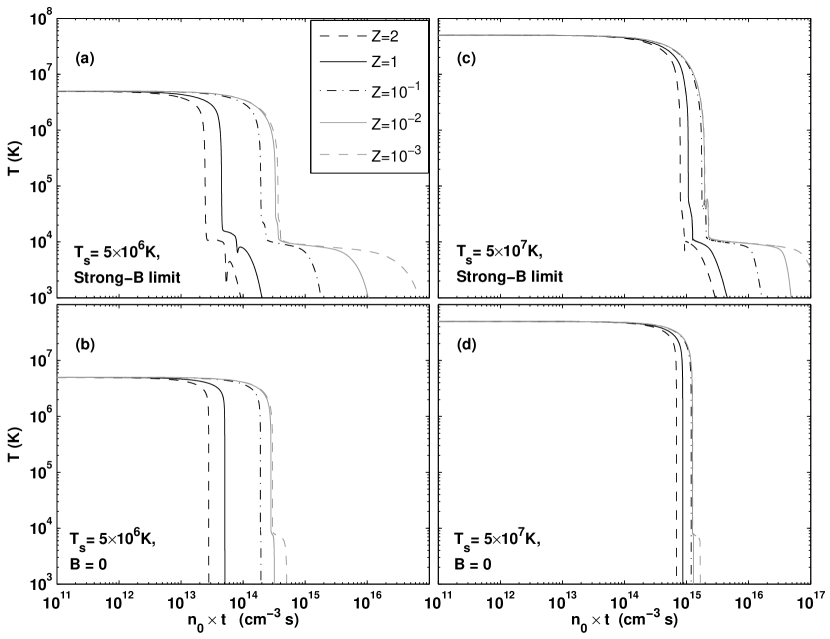
Figure 1.— Temperature versus post-shock hydrogen density times time (cm^-3 s), for gas metallicities ranging from $10^{-3}$ to $2$ times solar. The upper panels show results in the strong-$B$ limit (isochoric) and the lower panels show results for $B=0$ (approximately isobaric). The left hand panels show results for $T_{s}=5\times 10^{6}$ K, and the right hand panels for $T_{s}=5\times 10^{7}$ K. The results presented in this figure were computed assuming a post-shock hygrogen density, $n_{\rm H}=0.1$ cm^-3, but are nearly independent of density (see § 3.5).

3.1. A strong-$B$ (isochoric), $T_{s}=5\times 10^{6}$ K, shock at a metallicity of $Z=2$.

To illustrate the behavior of the post-shock cooling gas in the strong-$B$ limit, we first focus on the results for $T_{s}=5\times 10^{6}$ K and $Z=2$.

The initial ionization states of the gas that enters the shock, are set by photoionization equilibrium of the precursor gas with the shock self radiation. This gas has an equilibrium temperature which is significantly lower than the shock temperature.

As the precursor gas passes through the shock front, its temperature abruptly rises to $T_{s}$, leaving the gas under-ionized relative to CIE at the shock temperature. The gas then very rapidly adjusts to CIE at a temperature close to $T_{s}$. During this phase, the gas radiates very efficiently, as the hot thermal electrons efficiently excite the low-energy transitions of the under-ionized gas. Dopita and Sutherland (1996) refer to this phase as the “ionization zone”. The cooling efficiencies are about $60$ times higher than at CIE. The evolution to CIE is very rapid, and occurs within $n_{0}\times t=10^{11}$ cm^-3 s. After this time, the ion fractions and cooling efficiencies reach CIE, at a temperature very close to $T_{s}$ ($>0.95T_{s}$).

For the shock temperatures that we consider ($\gtrsim 5\times 10^{6}$ K), the CIE cooling efficiency at $\sim T_{s}$ is low. The gas therefore stays hot for a long time. This phase is the “hot radiative zone” (e.g. Draine & McKee 1993; Dopita & Sutherland 1996). Metal line emissions (and bremsstrahlung emission for low gas metallicity) dominate the cooling in this zone (Sutherland & Dopita 1993; GS07; see § 5).

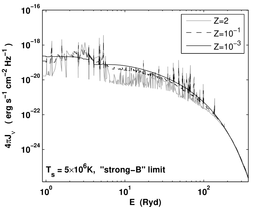
Figure 2.— Emitted mean intensity (erg s^-1 cm^-2 Hz^-1) versus energy (Ryd) for $T_{s}=5\times 10^{6}$ K in the strong-$B$ (isochoric) limit. The gray curve shows the emitted spectrum for $Z=2$, the dark dashed curve for $Z=10^{-1}$, and the dark solid curve for $Z=10^{-3}$.

The hot radiative phase ends once the gas cools to a temperature for which the cooling efficiency is high, $T\lesssim 10^{6}$ K. The shocked gas therefore emits most of its initial thermal energy while in the hot radiative phase. Figure 2 shows the mean intensity of the radiation field emitted by the shocked gas. The gray curve shows results for $Z=2$ times solar metallicity gas. For $Z=2$, the relative contribution of resonance lines is very large, and the line to continuum contrast is high. The spectrum shows a very prominent “UV-bump” created by numerous UV emission lines, with excess radiation between $\sim 1-5$ Ryd. The line contribution is also significant at far-UV and even X-ray energies. This radiation is absorbed by cooler gas further downstream, providing a source of heating and photoionization.

Once the temperature drops sufficiently to bring the gas closer to the cooling-efficiency peak, the temperature decline becomes very rapid, and the gas cools to a temperature of a few $\times 10^{4}$ K. If cooling becomes faster than recombination, departures from equilibrium occur, and the gas tends to stay over-ionized (Sutherland & Dopita 1993; GS07). We refer to this phase as the “non-equilibrium cooling zone” (e.g. Dopita & Sutherland 1996). During this rapid cooling stage, metal line emissions (and Hydrogen-Helium line emission for $Z\lesssim 10^{-2}$) dominate the cooling.

In Figure 3 we display various physical parameters in the cooling gas. The upper panel shows the temperature as a function of (linear) time, starting at the non-equilibrium cooling zone. As the gas cools, hydrogen starts to recombine (see panel c). Eventually, the neutral hydrogen fraction is high enough that it allows for efficient absorption of the shock radiation. This occurs when $x_{\rm H~{}I}\sim 10^{-3}$. This significantly raises the heating rate, as is shown by the gray line in panel (e). The integrated H I column density measured from the shock front is shown in panel (d).

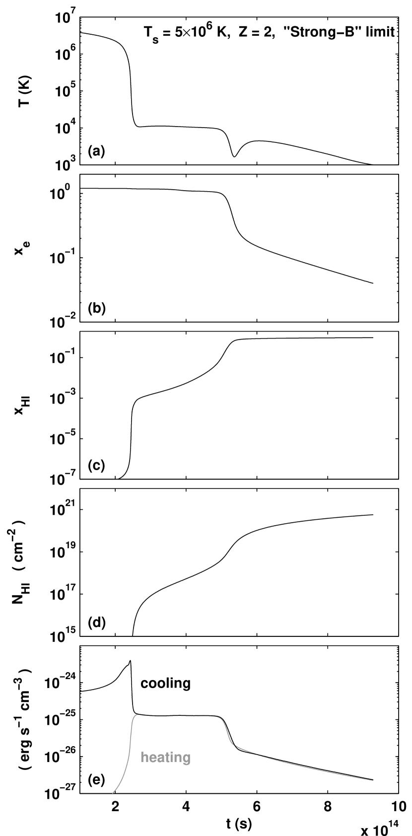
Figure 3.— Shock structure versus time for $T_{s}=5\times 10^{6}$ K, for $Z=2$ solar, and for a post-shock hydrogen density $n_{0}=0.1$ cm^-3, in the strong-$B$ limit. (a) Temperature (K). (b) Electron fraction. (c) Neutral hydrogen fraction. (d) Integrated H I column density (cm^-2) from the shock front. (e) Local cooling (dark) and heating (gray) rates per volume (erg s^-1 cm^-3).

Once the heating rate reaches the cooling rate (see panel e), the rapid temperature decrease stops, and the gas enters a “plateau” in which the temperature remains roughly constant, and the radiation is gradually absorbed. This is the “photoabsorption plateau” (e.g. Dopita & Sutherland 1996; also called the “recombination zone” [Shull & McKee 1979] or the “thermalization zone” [Draine & McKee 1993]). As the radiation is removed by absorption, the neutral fraction of the gas rises. In this optically thin and ionized part of the plateau, the heating rate changes very slowly. Once the neutral fraction is of order unity ($\gtrsim 0.1$), the optical depth increases and the heating rate declines more rapidly. We refer to the part of the plateau in which hydrogen is still ionized as the warm ionized medium (WIM) plateau.

The depth of the “WIM plateau” depends on the flux, $F_{\nu}$, of ionizing radiation entering the plateau. The thickness of the ionized region will be

$$l_{\rm WIM}=\frac{1}{n_{H}n_{e}\alpha}\int\frac{F_{\nu}}{h\nu}~{}d\nu,$$ (10)

where $\alpha$ is the recombination coefficient. The time spent in the WIM plateau is then $t_{\rm WIM}=l_{\rm WIM}/v_{0}\simeq 2.5\times 10^{14}$ s, following a $5\times 10^{6}$ K, $v_{0}=v_{s}/4=150$ km s^-1, $n_{0}=0.1$ cm^-3 isochoric shock.

For the set of parameters considered here ($T_{s}=5\times 10^{6}$ K, $Z=2$ solar, strong-$B$), after the hydrogen recombines the gas rapidly cools down to a temperature $T_{\rm low}=1000$ K, at which we terminate the computation. For other (lower) gas metallicities, an additional warm neutral medium (WNM) plateau may form, with a temperature between $8000$ and $10,000$ K. The depth of the “WNM plateau” depends on the gas X-ray opacity, which is set by the gas metallicity. The WNM plateau is more extended for lower metallicity gas (see Figure 1).

The various components in post-shock cooling layers (e.g. Draine & McKee 1993; Dopita & Sutherland 2003) are illustrated schematically in Figure 4. Here we have made the further distinction between warm ionized (WIM) and warm neutral (WNM) plateaus in the downstream absorbing layers.

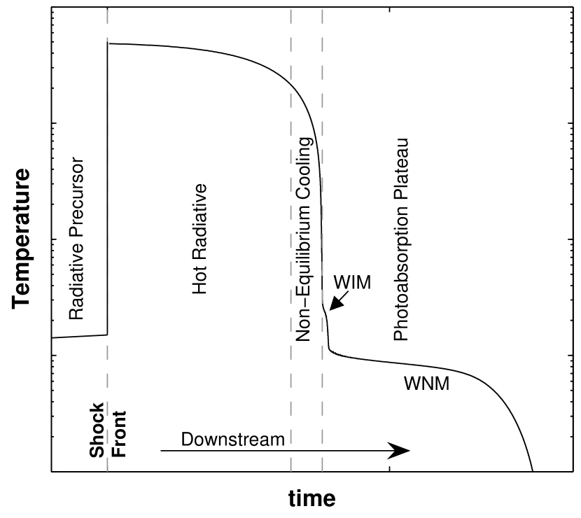
Figure 4.— A schematic plot of shock temperature versus time. The different zones are shown (from left to right): The preshocked upstream gas is initially in a photoionized “radiative precursor”; After passing the shock front, the gas enters the “Hot Radiative” zone, in which cooling is slow. It later passes through the “Non-Equilibrium Cooling” zone, in which cooling is rapid, and departures from equilibrium ionization and cooling may occur. After the neutral ion fraction rises, photoabsorption heating becomes efficient, and the gas enters a “Photoabsorption Plateau”, consisting of WIM and WNM components, in which the temperature declines much more slowly. Finally the gas cools to the minimal computed temperature. See text.

Throughout most of the photoabsorption plateau and the final cooling following it, the radiation field is absorbed slowly enough that the gas has time to approach photoionization and thermal equilibrium. The photoabsorption time scale is given by $t_{abs}=\frac{1}{<n\sigma>v}$, and the recombination time scale by $t_{rec}=\frac{1}{n_{e}\alpha}$. As long as $t_{rec}<<t_{abs}$, the gas stays at a state of near photoionization equilibrium with the local radiation field.

Once the temperature drops below $\sim 10^{4}$ K, Ly$\alpha$ emission and other allowed transitions become very inefficient, and the gas cools primarily via fine-structure (FS) line emissions, including O III 88.3$\mu$m, O III 51.8$\mu$m, Ne III 15.5$\mu$m, Si II 34.8$\mu$m, S III 33.5$\mu$m, and C II 157.7$\mu$m. (We do not include molecules or dust in this computation).

As mentioned above, for $Z=2$ metal line cooling dominates throughout. Metal lines are important even for $T\sim 10^{4}$ K where Ly$\alpha$ cooling dominates in CIE. The Ly$\alpha$ cooling efficiency is suppressed because the hydrogen is still mostly ionized, while the existence of over-ionized metal species, such as Ne⁴⁺, O³⁺, S³⁺, allows for efficient line cooling that is not available in CIE. Initially, the heating in the plateau is due to H I photoionization (for $n_{0}\times t<5.3\times 10^{13}$ cm^-3 s), then He I photoionization (for $5.3\times 10^{13}<n_{0}\times t<7.4\times 10^{13}$ cm^-3 s), and then by photoionization of metals, mostly by neutral oxygen (for $n_{0}\times t>7.4\times 10^{13}$ cm^-3 s). These transitions occur as the photo-absorptions remove lower energy photons from the radiation field. For photon energies greater than $1.8$ Ryd, helium absorbs more efficiently than hydrogen, and at yet higher energies oxygen is more efficient than helium.

Below $\sim 10^{4}$ K, the cooling rate per volume generally decreases due to the decreasing electron density. Below $\sim 6000$ K, the cooling rate per electron ($n_{H}\Lambda$) is constant to within  30% (for $Z=2$), with small variations due to recombinations that increases the abundance of the dominant coolants (e.g. C II 157.7$\mu$m and Si II 34.8 $mu$m).

Because the radiation field controls both the heating rate, and the electron fraction (which influences the cooling rates), heating and cooling remain strongly coupled for the remainder of the cooling process. While both the heating and cooling rates decrease with time, they remain nearly equal, leading to the slow thermal evolution in the plateau. However, departures from exact thermal equilibrium enable the gas to cool further, down to a temperature of $1650$ K at $n_{0}\times t~{}\sim 5.4\times 10^{13}$ cm^-3 s.

As the gas cools, and the heating radiation is absorbed, the H and He preferentially absorb low energy photons, and the remaining ionizing radiation therefore becomes harder with increasing depth in the photoabsorption plateau. Figure 3e shows that after the UV photons are absorbed (at $t\sim 5\times 10^{14}$ s), the heating rate decreases much more rapidly, and the cooling rate lags slightly behind the heating. This leads to the brief temperature dip at $n_{0}\times t=5.4\times 10^{13}$ s cm^-3 in Fig. 3a. After reaching a temperature minimum of $1650$ K at this time, the gas heats up again to $\sim 4500$ K. After this, the cooling rate overcomes the heating rate again, and the gas then cools monotonically to $1000$ K where we terminate the computation.

The shock structure and time-scales that are shown in Figure 1 are in qualitative agreement with previous computations (Dopita & Sutherland 1996, Allen et al. 2008). For example, our results for the temperature profiles in a solar metallicity shock, are similar to those presented in Allen et al. (2008) for their “Dopita 2005” abundance set (middle panel of their Figure 7), where gas stays in the hot radiative phase for a few $\times 10^{13}$ s, and then rapidly cools through the non-equilibrium cooling zone to enter the photoabsorption plateau. Differences between our results and those of Allen et al. are likely due to differences in the assumed abundances, and in the strength of the magnetic field, $B$.

3.2. Dependence on Gas Metallicity

The time-scale over which the gas cools from the initial shock temperature down to $1000$ K, depends on the shock velocity that sets the initial energy content of the shocked gas, and on the cooling efficiency of the post-shock gas. For $T_{s}=5\times 10^{6}$ K, the cooling is initially dominated by metal resonance line cooling for $Z\gtrsim 0.1$, and by bremsstrahlung emission for $Z\lesssim 10^{-2}$. For $T_{s}\gtrsim 10^{7}$ K, bremsstrahlung cooling becomes important even for high-metallicity gas. Metal lines continue to dominate the cooling at lower temperature for $Z\gtrsim 0.1$, whereas for $Z\lesssim 0.1$, hydrogen and helium dominate the cooling at $T\lesssim 3\times 10^{5}$ K (see also GS07).

The cooling efficiency therefore strongly depends on the metal content within the gas. For $Z\gtrsim 0.1$, the cooling efficiency is roughly proportional to the gas metallicity. However, at lower gas metallicity, as the metal contribution to the cooling rate above $\sim 10^{4}$ K becomes negligible, the cooling efficiency approaches a limit set by the primordial helium abundance (see Boehringer & Hensler 1989; GS07). This can be seen in Figure 1. For high gas metallicities the cooling time is proportional to $Z$, whereas the curves for $Z=10^{-2}$ and for $Z=10^{-3}$ nearly overlap for temperatures above $10^{4}$ K.

For $Z>1$, even at $\sim 10^{4}$ K, permitted metal transitions dominate the cooling, and are much more efficient than Ly$\alpha$. For $Z=1$ Ly$\alpha$ provides $\sim 15\%$ of the cooling at its peak efficiency. For lower gas metallicities, Ly$\alpha$ provides most of the cooling at $T\sim 10^{4}$ K. For example, for $Z=0.1$, Ly$\alpha$ provides as much as $80\%$ of the cooling. Therefore, the cooling times at $\sim 10^{4}$ K are nearly independent of gas metallicity, except for $Z>1$.

As the gas cools below $\sim 10^{4}$ K, metal fine structure emissions start to dominate the cooling, even for the lowest gas metallicities. In addition, the gas opacity and associated depth over which the heating radiation is absorbed are functions of the gas metallicity. The cooling times below $\sim 10^{4}$ K are roughly proportional to gas metallicity for all $Z$. The overall total cooling times in isochoric flows is therefore sensitive to $Z$, as can be clearly seen in panel (a) of Figure 1.

The different cooling times also set the degree of non-equilibrium ionization in the gas (GS07), as affected by the ratio of the cooling-time and the (metallicity-independent) recombination time. When the cooling is faster than recombination, departures from equilibrium may occur. Since cooling is faster for high gas metallicities, non-equilibrium effects, and the over-ionization in the gas, are more important for higher $Z$. These effects occur at temperatures between $\sim 10^{6}$K and $10^{4}$ K where the cooling is rapid. Below $10^{4}$ K, the heating becomes efficient, and the cooling times becomes long, so that the gas stays close to photoionization equilibrium.

A second factor that is strongly affected by the gas metallicity is the radiation field emitted by the cooling gas. As discussed before, the emitted radiation is composed mainly of bremsstrahlung continuum, and of emission-lines and recombination continua. The total flux of radiation emitted by the cooling gas equals the input energy flux into the flow,

$$F\propto n_{0}k_{\rm B}T_{s}v_{s}\propto n_{0}v_{s}^{3}\ \ \ .$$ (11)

However, the relative contribution of metal emission lines to the total flux depends on $Z$.

For high-metallicity gas, a large fraction of the input energy is radiated as line emission. For low metallicity, the relative contribution of lines is small, and most of the initial energy flux is radiated as thermal bremsstrahlung. This can be clearly seen in Figure 2. For $Z=2$ (the gray solid line), the lines-to-continuum contrast is large, producing the “UV-bump” discussed above. For $Z=0.1$ (dashed dark curve), lines are still important, but are much less pronounced than for $Z=2$. For $Z=10^{-3}$ (black solid curve) the spectrum is very smooth, and consists almost entirely of thermal bremsstrahlung.

The differences in the spectral energy distribution of the emitted radiation field affect the thermal evolution of the cooling gas in the photoabsorption region, and the resulting ion distributions. We discuss the impact of the changing spectral energy distribution on the ion fractions in detail in § 4.

Additional features in the shock profiles are affected by the gas metallicity and associated cooling efficiency. The start of the photoabsorption plateau is associated with the increase in photoabsorption efficiency that occurs as the neutral hydrogen fraction becomes sufficiently large (of order $10^{-3}$ for $5\times 10^{6}$ K shocks). Higher-metallicity gas is more over-ionized, and therefore reaches this critical neutral fraction at a lower temperature. The start of the WIM plateau therefore takes place at lower temperature for higher metallicity gas. For $Z=2$, the plateau starts at $10^{4}$ K, for $Z=1$ at $1.7\times 10^{4}$ K, and for $Z\lesssim 0.1$ at $2.5\times 10^{4}$ K. The depth of the WIM plateau is given by equation (10). Since the energy flux emitted by models with the same initial shock temperature and magnetic field is similar, the depth of the WIM plateau is independent of gas metallicity. For our $T_{s}=5\times 10^{6}$ K shocks it is $\sim 2.5\times 10^{14}$ s (for $n_{0}=0.1$ cm^-3 and strong-$B$) for $Z$ between $10^{-3}$ and $2$.

For $Z<1$, a second warm ionized medium plateau is apparent in Figure 1. This plateau has a temperature $T\sim 10^{4}$ K. The depth over which the heating self-radiation is absorbed and the WNM plateau persists, depends on the gas opacity which is a function of $Z$. Lower metallicity gas produces longer WNM plateaus.

In the final cooling of the gas, fine-structure transitions dominate the cooling. The intensity of fine-structure cooling is proportional to gas metallicity as discussed above. At high gas metallicities ($Z\gtrsim 1$) fine-structure cooling is efficient, and starts to dominate the cooling at $\sim 10^{4}$ K. At lower metallicities ($Z\lesssim 0.1$), fine-structure cooling starts to dominate at $\sim 7500$ K.

3.3. Shock Temperature

Panel (c) of Figure 1 shows the temperature profiles in a shock with an initial temperature $T_{s}=5\times 10^{7}$ K, in the strong-$B$ limit. The overall characteristics of these temperature profiles are similar to those of the lower-velocity ($T_{s}=5\times 10^{6}$ K) shocks discussed in § 3.1. The gas is initially heated to $T_{s}$, then goes through a prolonged hot radiative phase during which it emits most of its initial thermal energy as radiation. As $T$ drops, cooling becomes more efficient, and a phase of rapid non-equilibrium cooling begins, bringing the gas to a temperature of a few $\times 10^{4}$ K. At this point the neutral hydrogen fraction becomes large enough that photoionization heating becomes significant, and a temperature plateau is formed. The WIM plateau ends when the neutral fraction is of order unity. A WNM plateau then follows. The gas finally cools to our cut-off temperature, $T_{\rm low}=1000$ K.

Since the initial temperature is $10$ times higher in a $5\times 10^{7}$ K shock than in a $5\times 10^{6}$ K shock, and the velocity is $10^{1/2}\sim 3$ times higher, the total energy flux input is $\sim 30$ times higher. The overall cooling time is therefore longer, as the gas has to radiate more energy.

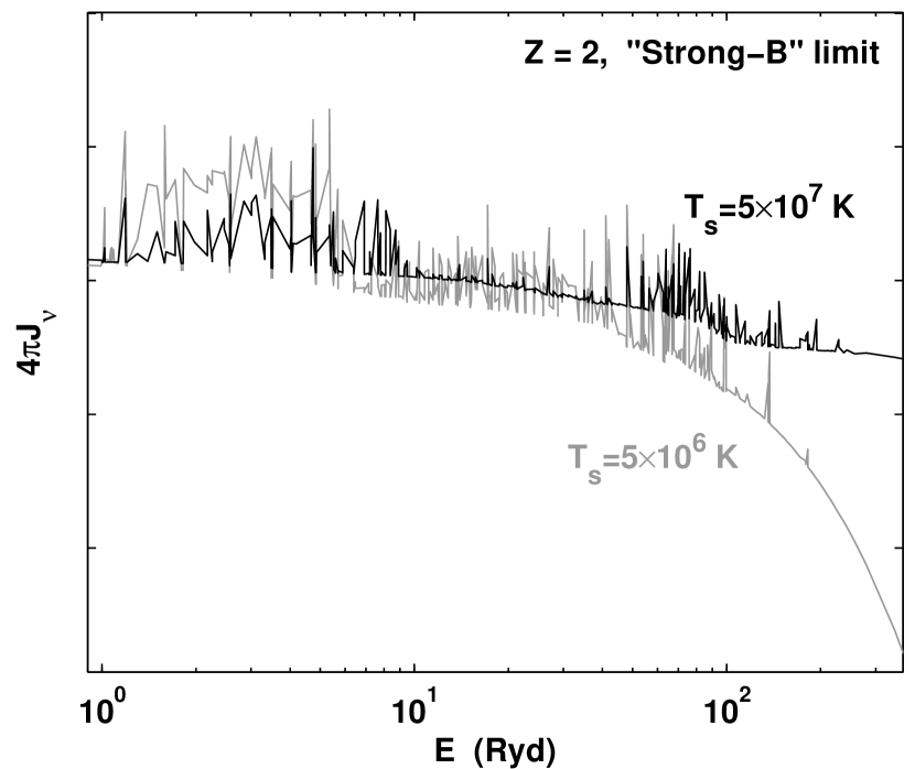
Figure 5.— Shock self-radiation as a function of shock temperature for the strong-$B$ limit, and for $Z=2$. The dark curve is the mean intensity (erg s^-1 cm^-2 Hz^-1) for $T_{s}=5\times 10^{6}$ K. The gray curve is the mean intensity for $T_{s}=5\times 10^{7}$ K. The spectra are normalized so that their UV continuum-intensities overlap, to emphasize the different spectral energy distributions.

The emitted radiation field is affected by the increased initial temperature. The higher temperature produces a more intense bremsstrahlung continuum with more energetic photons (the exponential bremsstrahlung cut-off occurring at higher photon frequencies). In addition, since at temperatures above $\sim 2\times 10^{7}$ K bremsstrahlung is the dominant cooling process even at $Z=2$, a large fraction of the initial energy is radiated as bremsstrahlung continuum rather than in lines. Lines still dominate the cooling at lower temperatures, but their total contribution to the integrated spectrum is smaller. This is shown in Figure 5 that compares the (normalized) spectral energy distributions for $5\times 10^{6}$ K and $5\times 10^{7}$ K shocks. The hotter shock provides a flatter spectrum extending to higher energies, and its line-to-continuum contrast is smaller due to the larger fraction of radiation emitted at high temperatures dominated by bremsstrahlung emission.

Because much of the initial energy in the $5\times 10^{7}$ K shock gas is radiated as bremsstrahlung, the cooling times above $\sim 10^{4}$ K are much less sensitive to the gas metallicity than for $5\times 10^{6}$ K-shocks. In fact, the cooling time from $5\times 10^{7}$ K to $\sim 10^{4}$ K increases only by a factor of $1.6$ when the metallicity is reduced from $Z=1$ to $Z=0.1$.

3.4. Magnetic Field

Panel (b) of Figure 1 shows the temperature profiles for $T_{s}=5\times 10^{6}$ K, assuming $B=0$. As discussed in § 2.2, the hydrodynamics follow equations (3), and the evolution is nearly isobaric, with $P_{\infty}=4/3\;P_{0}$. The most important difference between shocks in which $B=0$ and the previously discussed strong-$B$ limit, is that for $B=0$ the density increases as the gas cools. Since the cooling time is inversely proportional to the gas density, this implies a rapidly decreasing cooling time within the flow. The overall cooling times are therefore much shorter, and the evolution below $10^{4}$ K, while qualitatively similar to that of the previously discussed isochoric shocks, is compressed into a very short interval. This can be seen in Figure 1b. Once the gas starts to cool, the decline down to a temperature of $1000$ K is very rapid.

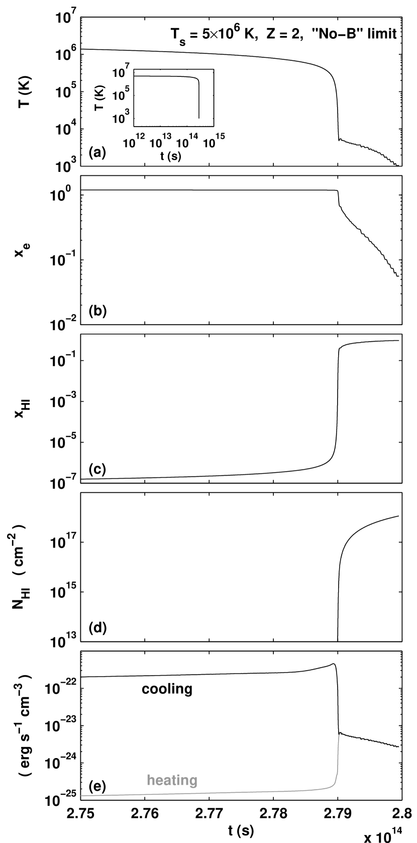
Figure 6.— Shock structure versus time for $T_{s}=5\times 10^{6}$ K, $Z=2$ solar, for $B=0$. The plots focus on the final evolution, between $2.75\times 10^{14}$ s and $2.8\times 10^{14}$ s for $n_{0}=0.1$ cm^-3. (a) Temperature (K). (b) Electron fraction. (c) Neutral hydrogen fraction. (d) Integrated H I column density (cm^-2) from the shock front. (e) Local cooling (dark) and heating (gray) rates per volume (erg s^-1 cm^-3).

Figure 6 shows a “zoomed-in” snapshot of the final stages of the evolution for $Z=2$. All times are shown assuming a post shock hydrogen density of $0.1$ cm^-3. The insert in panel (a) shows the full temperature profile in the flow. The panels focus on the final evolution, between $t=2.75\times 10^{14}$ s and $2.8\times 10^{14}$ s. The final evolution shows similar features to those discussed for the strong-$B$ isochoric shocks. The gas cools rapidly to a point where photoabsorption becomes significant enough that the heating balances the cooling. It then enters a photoabsorption region in which the shock self-radiation is gradually absorbed, and the temperature decline becomes slower. This happens on much shorter time scales due to the increasing density (c.f. Figure 5 in Allen et al. 2008).

Equation (11) states that the total flux created by the cooling gas is proportional to the input energy flux, $F\propto n_{0}v_{s}^{3}$. Almost all of this flux ($>99.8\%$) is emitted before the plateau starts, and most of it ($>80\%$) is emitted within the hot radiative zone. The level of photoionization in the gas is determined by the ionization parameter, which is proportional to $F/n$. For strong-$B$ shocks, the density in the flow is constant, and the ionization parameter is therefore $\propto v_{s}^{3}$. For $B=0$, the density increases as the gas cools, and the ionization parameter is therefore $\propto v_{s}^{3}n_{0}/n$, which is smaller by a factor $n_{0}/n$ (or $\sim T/T_{s}$). Photoionization is therefore much less important in $B=0$ models, and its contribution to the creation of intermediate- and high-ions is diminished.

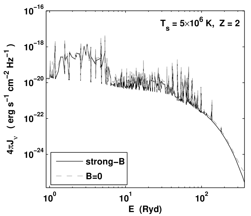
Figure 7.— Shock self radiation for $T_{s}=5\times 10^{6}$ K shocks and for $Z=2$ solar metallicity gas. The solid curve shows the mean intensity (erg s^-1 cm^-2 Hz^-1) in the strong-$B$ limit. The gray dashed curve shows the mean intensity for $B=0$, divided by $5/3$ to remove the $PdV$ contribution. As expected, the spectra are similar.

A more subtle effect is related to the $PdV$ work that appears in $B=0$ shock models, due to the gas compression. The work done on the cooling gas implies that the overall emitted radiation field is $5/3$ times larger for $B=0$ shocks than for isochoric shocks (Edgar & Chevalier 1986; GS07). The final total flux in strong-$B$ flows is $3/2~{}n_{0}k_{\rm B}T_{s}v_{s}$, while for $B=0$ it is $5/2~{}n_{0}k_{\rm B}T_{s}v_{s}$. This is shown in Figure 7. However, the effect of the $5/3$-factor on the downstream ionization parameter is much smaller than the impact of the increasing density in $B=0$ shocks.

Figure 8 compares the temperature profiles for strong-$B$ and $B=0$ models. Initially, due to the $PdV$ work, the cooling in the isochoric, strong-$B$, shock is faster than in the $B=0$ nearly isobaric flow. However, for $B=0$ the density and cooling rates quickly grow, and the final $B=0$ cooling is much more rapid.

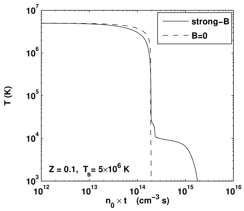
Figure 8.— Temperature profiles for $T_{s}=5\times 10^{6}$ K and $Z=0.1$ solar metallicity. The solid curve shows results in the strong-$B$ limit. The dashed curve shows results for $B=0$.

Figure 9 shows the hydrodynamic evolution of a $B=0$, $T_{s}=5\times 10^{6}$ K, $Z=2$ flow. Panel (a) shows the gas temperature. Panel (d) shows the gas pressure. As discussed above (see equation [5]), the flow is nearly isobaric, with a total pressure change of $4/3$. This implies that the gas density is roughly inversely proportional to the temperature, as can be seen in panel (b). The mass flux conservation equation implies that the velocity is inversely proportional to the gas density as can be seen in panel (c).

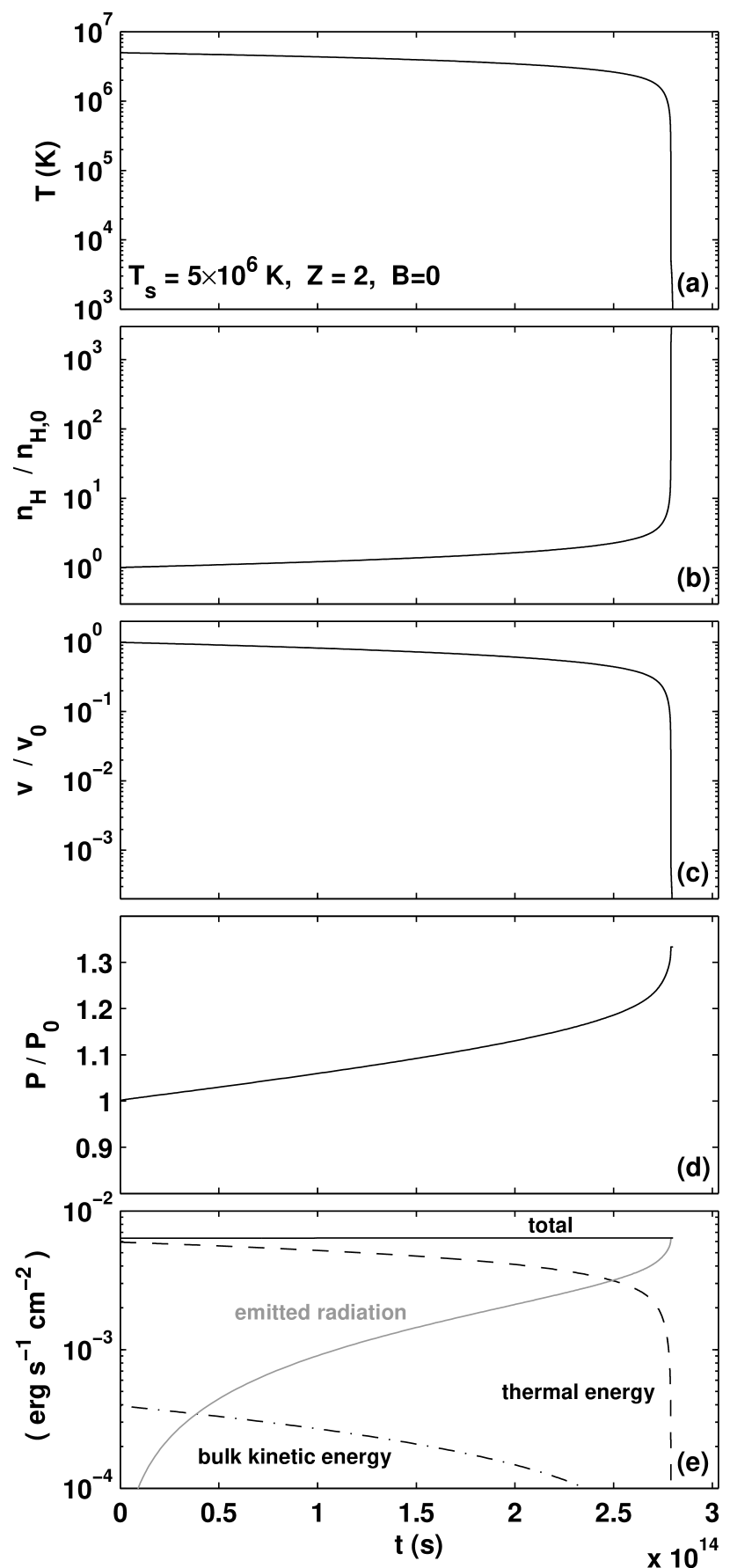
Figure 9.— Dynamics in a $5\times 10^{6}$ K, $Z=2$, $B=0$ shock. (a) Temperature (K). (b) Density profile. (c) Velocity profile. (d) Pressure profile. (e) Energy flux (erg s^-1 cm^-2). The dark solid curve shows the total energy flux in the flow, which is conserved as it should. The dashed line shows the thermal energy flux ($\frac{5}{2}Pv$), which is initially the dominant component of the energy flux, but drops as the gas cools. The dash-dotted line shows the bulk kinetic energy flux ($\frac{1}{2}\rho v^{3}$). The gray solid curve is the integrated cooling radiation, which is accumulated in the flow as the gas cools, until it reaches the total input energy flux when all thermal energy is lost.

For $B=0$, the pressure is dominated by the thermal gas pressure through the flow. We can therefore verify mass, momentum and energy conservation, and we indeed find that they are conserved to better than $1\%$. Panel (e) shows the energy flux components in the flow. The total energy flux, shown by the upper solid line, remains constant as it should. The thermal energy component ($5Pv/2$) is shown by the dark dashed line. Initially it dominates the energy flux, but as the gas cools, the thermal component gradually decreases. The bulk kinetic energy ($\rho v^{3}/2$) is shown by the dash-dotted line. Initially, this is only a small fraction of the total energy flux, and it decreases further as the gas cools and decelerates. The gray line shows the integrated cooling radiation. As expected, this component grows with depth into the flow, and finally reaches a value equal to the total initial energy flux when all internal thermal energy is lost.

The impact of gas metallicity on $B=0$ isobaric shocks is similar to that which occurs in strong-$B$ isochoric shocks discussed in § 3.2. Again, as the gas metallicity increases, the metal-line cooling efficiency increases, and cooling becomes more rapid. This is clearly seen in Figure 1b, where the initial cooling time is proportional to gas metallicity, except at $Z\lesssim 10^{-2}$ where the metals contribution to the cooling is negligible.

The cooling below $\sim 10^{4}$ K is very rapid due to the increased gas density. While the cooling times below $\sim 10^{4}$ K are proportional to gas metallicity, this cannot be seen in Figure 1b since the total cooling times below $\sim 10^{4}$ K are so much shorter than the cooling times from $5\times 10^{6}$ K to $10^{4}$ K. The low-temperature cooling time only becomes long enough to be seen in Figure 1b for $Z\lesssim 10^{-2}$, for which the cooling time during the plateau phase is of order the cooling time to reach the plateau.

3.5. Gas Density

The results discussed above for $T$ versus $n_{0}\times t$ are independent of density for strong-$B$ isochoric models. When $B=0$, the gas is compressed as it cools, and the thermal evolution below $\sim 10^{4}$ K may depend on the initial density. In the high-density compressed gas, the cooling efficiencies may be suppressed by collisional de-excitations of the cooling transitions if the densities become sufficiently high. The temperature at which such collisional quenching occurs depends on the shock velocity as well as on the initial post-shock density, $n_{0}$.

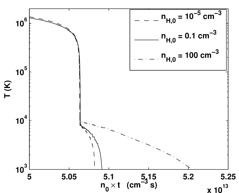
Figure 10.— Temperature profiles for different post-shock hydrogen densities, for a $5\times 10^{6}$ K shock and $B=0$. The plot focuses on the final evolution. Higher density models cool less efficiently because collisional quenching occurs sooner as the gas is compressed.

Figure 10 shows the temperature as a function of $n_{0}\times t$ in $T_{s}=5\times 10^{6}$ K shocks, assuming post-shock hydrogen densities of $10^{-5}$ cm^-3 (dashed line), $0.1$ cm^-3 (solid line), and $100$ cm^-3 (dash-dotted line). For these initial densities, the gas density never becomes high enough for significant collisional de-excitation of the permitted transitions. However, once the temperature drops below $\sim 10^{4}$ K, some of the fine-structure cooling is quenched, and the thermal evolution is altered. As shown by Figure 10, for higher initial post-shock densities this collisional quenching occurs sooner, and the effective cooling times, $n_{0}\times t$, are therefore longer for higher $n_{0}$ (c.f. Figure 6 in Allen et al. 2008, in which the cooling times from $T_{s}$ to the photoabsorption plateau scale as $n^{-1}$, whereas the cooling below $\sim 10^{4}$ K depends more strongly on $n$).

3.6. Steady-State Conditions

The results presented in this paper rely on the assumption that the shocks have reached a steady-state structure. Attaining steady-state requires that the shock exists for a time-scale that is longer than the cooling time. Otherwise, the shocked gas only cools partially, and the shock structure, self-radiation, and integrated column densities are time-dependent.

In Table 2 we list the total cooling times (yr), from $T_{s}$ down to $1000$ K, assuming a post-shock hydrogen density, $n_{0}=1$ cm^-3. We also list the associated length-scales (kpc), and total hydrogen column densities, $N_{\rm H,tot}$ (cm^-2). These are then the hydrogen columns and length scales required for the formation of steady-state shocks. For example, Table 2 implies that for a $T_{s}=5\times 10^{6}$ K shock in solar metallicity gas, the time required to reach steady-state is $6.4\times 10^{6}$ yrs, in the strong-$B$ isochoric limit. The cooling length is then $1$ kpc, and the associated hydrogen column density is $3\times 10^{21}$ cm^-2. The time- and size-scales are generally proportional to $n_{0}^{-1}$, while the total hydrogen columns are generally independent of $n_{0}$ (but see § 3.5).

Table 2Shock Parameters (for $n_{0}=1$ cm^-3)

	$T_{s}=5\times 10^{6}$ K				$T_{s}=5\times 10^{7}$ K
Metallicity	Time	Size	$N_{\rm H,tot}$		Time	Size	$N_{\rm H,tot}$
	(yr)	(kpc)	(cm-2)		(yr)	(kpc)	(cm-2)
strong-$B$ (isochoric)
$Z=2$	$2.9\times 10^{6}$	$0.45$	$1.4\times 10^{21}$		$9.2\times 10^{7}$	$45$	$1.4\times 10^{23}$
$Z=1$	$6.4\times 10^{6}$	$1.0$	$3.0\times 10^{21}$		$1.4\times 10^{8}$	$71$	$2.2\times 10^{23}$
$Z=10^{-1}$	$5.7\times 10^{7}$	$8.8$	$2.7\times 10^{22}$		$5.2\times 10^{8}$	$250$	$7.8\times 10^{23}$
$Z=10^{-2}$	$3.3\times 10^{8}$	$50$	$1.6\times 10^{23}$		$1.5\times 10^{9}$	$750$	$2.3\times 10^{24}$
$Z=10^{-3}$	$2.1\times 10^{9}$	$330$	$1.0\times 10^{24}$		$4.1\times 10^{9}$	$2000$	$6.3\times 10^{24}$
$B=0$ (“isobaric”)
$Z=2$	$8.9\times 10^{5}$	$0.10$	$4.3\times 10^{20}$		$2.2\times 10^{7}$	$7.0$	$3.3\times 10^{22}$
$Z=1$	$1.6\times 10^{6}$	$0.18$	$7.8\times 10^{20}$		$2.8\times 10^{7}$	$8.6$	$4.2\times 10^{22}$
$Z=10^{-1}$	$6.1\times 10^{6}$	$0.63$	$2.9\times 10^{21}$		$3.8\times 10^{7}$	$11.0$	$5.7\times 10^{22}$
$Z=10^{-2}$	$1.0\times 10^{7}$	$0.87$	$4.8\times 10^{21}$		$4.1\times 10^{7}$	$11.4$	$6.3\times 10^{22}$
$Z=10^{-3}$	$1.6\times 10^{7}$	$0.91$	$7.7\times 10^{21}$		$5.3\times 10^{7}$	$11.5$	$8.0\times 10^{22}$

Note. — Cooling-times (yr), size-scales (kpc), and total hydrogen column densities (cm^-2) for post-shock gas cooling from $T_{s}$ to $1000$ K, assuming a post-shock hydrogen density, $n_{0}=1$ cm^-3.

4. Ion Fractions

We have computed the ionization states of H, He, C, N, O, Ne, Mg, Si, S, and Fe in the post-shock cooling layers. When the photoionized precursor-gas enters the shock, its ionization state rapidly reaches CIE at a temperature very close to $T_{s}$. As the hot gas flows away from the shock front, it recombines, cools, and radiates away its thermal energy. This radiation is later absorbed by the cooler gas further downstream, providing a source of heating and photoionization. We follow the time dependent ion fractions in the flow, taking into account photoionization by the shock self-radiation. As we discuss below, the photoionizing radiation significantly affects the ion fractions in the gas.

When the cooling time becomes short compared to the recombination time, departures from equilibrium may occur, keeping the gas over-ionized compared to ionization equilibrium at the local conditions (as specified by the mean intensity of the photoionizing radiation, gas density, and temperature). We consider the non-equilibrium ionization states as a function of the time dependent temperature and mean radiation intensity. We present results for gas cooling behind shocks with initial post-shock temperatures $5\times 10^{6}$ K and $5\times 10^{7}$ K, with metallicities $Z=10^{-3}$, $10^{-2}$, $10^{-1}$, $1$, and $2$ times the solar metal abundances, in the $B=0$ (nearly isobaric) and “strong-$B$” (isochoric) limits.

Table 3 lists the ion fractions as a function of time and temperature for the various models that we consider, as outlined in Table 4. All the times given in Table 3 were computed assuming a post-shock hydrogen density $n_{{\rm H},0}=0.1$ cm^-3. As we discussed in § 3, the shock structures, as functions of $n_{0}\times t$, are independent of the gas density in the strong-$B$ limit, and are density-dependent only at low temperatures ($\lesssim 10^{4}$ K) when $B=0$.

Table 3Ion Fractions in a $5\times 10^{6}$ K, $2$ times solar, strong-$B$-shock

Time	Temperature	H0/H	H+/H	He0/He	…
s	K
$0.00$	$5.000\times 10^{6}$	$1.63\times 10^{-4}$	$0.00$	$4.93\times 10^{-3}$	…
$7.25\times 10^{8}$	$4.998\times 10^{6}$	$1.52\times 10^{-5}$	$0.00$	$3.59\times 10^{-3}$	…
$1.57\times 10^{9}$	$4.997\times 10^{6}$	$1.01\times 10^{-6}$	$0.00$	$2.48\times 10^{-3}$	…

Note. — The complete version of this table is in the electronic edition of the Journal. The printed edition contains only a sample. The full table lists ion fractions for the $B=0$ (isobaric) and strong-B (isochoric) magnetic field limits, for shock temperatures of $5\times 10^{6}$ K and $5\times 10^{7}$ K, and for $Z=10^{-3}$, $10^{-2}$, $10^{-1}$, $1$, and $2$ times solar metallicity gas (for a guide, see Table 4). The times in the first column are fo an assumed post-shock hydrogen density of $0.1$ cm^-3.

Table 4Ionization and Cooling Tables

					Post-Shock	Precursor
Data			Ion Fractions	Cooling	Columns	Columns
$5\times 10^{6}$ K	strong-$B$	$Z=2$	3A	5A	6A	8A
		$Z=1$	3B	5B	6B	8B
		$Z=10^{-1}$	3C	5C	6C	8C
		$Z=10^{-2}$	3D	5D	6D	8D
		$Z=10^{-3}$	3E	5E	6E	8E
	$B=0$	$Z=2$	3F	5F	6F	8F
		$Z=1$	3G	5G	6G	8G
		$Z=10^{-1}$	3H	5H	6H	8H
		$Z=10^{-2}$	3I	5I	6I	8I
		$Z=10^{-3}$	3J	5J	6J	8J
$5\times 10^{7}$ K	strong-$B$	$Z=2$	3K	5K	6K	8K
		$Z=1$	3L	5L	6L	8L
		$Z=10^{-1}$	3M	5M	6M	8M
		$Z=10^{-2}$	3N	5N	6N	8N
		$Z=10^{-3}$	3O	5O	6O	8O
	$B=0$	$Z=2$	3P	5P	6P	8P
		$Z=1$	3Q	5Q	6Q	8Q
		$Z=10^{-1}$	3R	5R	6R	8R
		$Z=10^{-2}$	3S	5S	6S	8S
		$Z=10^{-3}$	3T	5T	6T	8T

As a detailed example, in Figure 11 we show the carbon ion fractions for $T_{s}=5\times 10^{6}$ K, in the strong-$B$ limit, for the various values of $Z$. The second panel (Fig 11b) shows the results for $Z=1$. We first focus on these results, and then consider how the results depend on $Z$.

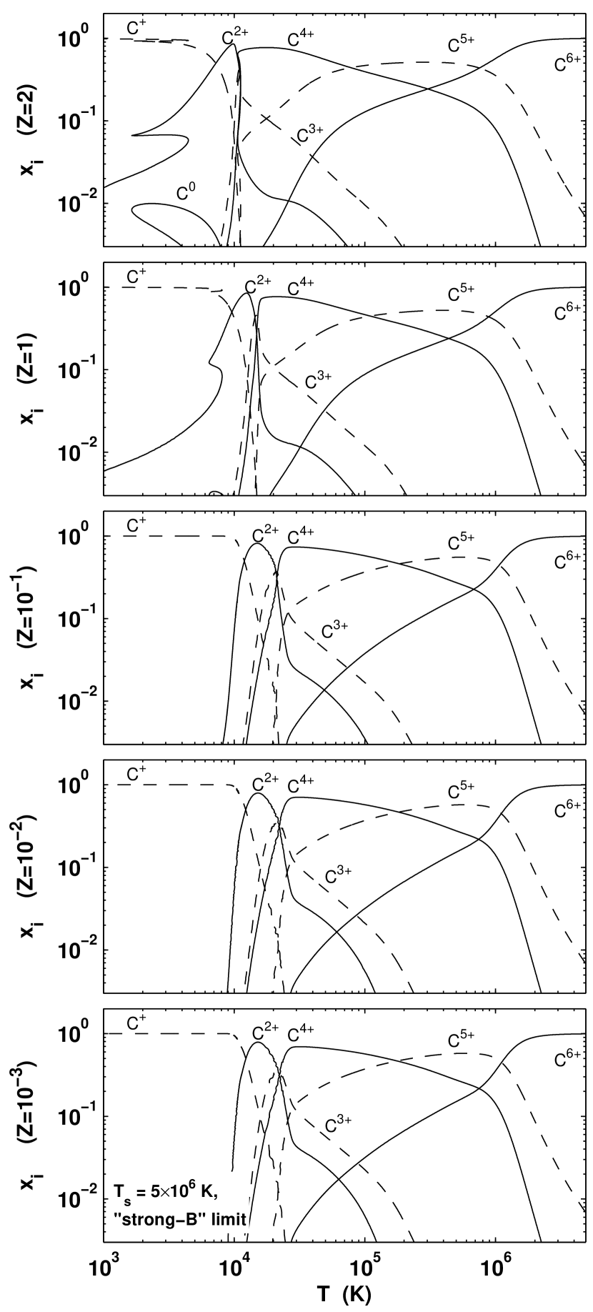
Figure 11.— Carbon ion fractions versus gas temperature in a $T_{s}=5\times 10^{6}$ K shock in the strong-$B$ limit. The various panels show results for gas metallicities ranging from $10^{-3}$ to $2$ times solar.

As the photoionized precursor gas enters the shock, the carbon ion fractions approach CIE at the shock temperature. This initial rise is very rapid, and cannot be seen in Figure 11. Figure 12 focuses on this initial evolution. The abundant carbon ions in the precursor gas are C⁴⁺ and C⁵⁺. As can be seen from Figure 12, these ionization states are quickly replaced by C⁶⁺, which is the abundant ion at $T_{s}=5\times 10^{6}$ K (see GS07). By the time the temperature drops to $4.97\times 10^{6}$ K, the carbon ion fractions reach CIE. Later on, as carbon recombines in the cooling flow, the lower ionization states reappear at lower temperatures, as can be seen in the second panel of Figure 11. For example, C⁴⁺ is again the most abundant carbon ion between $T\sim 10^{5}$ K, and $T\sim 2\times 10^{4}$ K. Many ionic species show such a double peak abundance pattern, where the abundance peaks first immediately after passing through the shock front, and then a second time as the gas recombines further downstream.

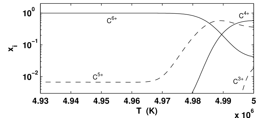
Figure 12.— Carbon ion fraction versus gas temperature just after crossing the shock front, for $T_{s}=5\times 10^{6}$ K, strong-$B$, and $Z=1$ gas. The plot shows how the initial ionization states quickly adjust to CIE at the initial shock temperature.

The time scales of the two peaks are very different. For the example shown is Figure 12, the width of the first peak in the C⁴⁺ abundance is of order $10^{12}$ s, while the second peak lasts of order $10^{14}$ s. The total contribution of the first abundance peak to the total ionic column density is therefore very small. However, since the gas is underionized as it goes through this first peak, the hot ambient electrons efficiently excite the transitions of the underionized ions (McCray 1987), creating an enhanced emissivity. This enhanced emissivity also implies that the cooling rates during this adjustment phase are enhanced. In lower velocity shocks, the first peaks can contribute significantly to the integrated column denisties (Krolik & Raymond 1985).

Figure 11 shows that in the hot radiative zone, the gas remains close to CIE, with C⁶⁺ being the most dominant carbon ion. During the non-equilibrium cooling phase ($T\lesssim 10^{6}$ K), the gas cools and recombines, and the most abundant ionization state drops to C⁵⁺ and later to C⁴⁺. The ionization state stays higher than at CIE due to photoionization by the shock self-radiation as we discuss below. The photoabsorption plateau starts at $T\sim 2\times 10^{4}$ K, and as the shock self radiation is absorbed within the plateau, the dominant carbon ion gradually drops from C³⁺ to C²⁺, and finally to C⁺. For the parameters considered here, C⁺ remains the dominant species until the gas reaches our termination temperature $T_{\rm low}=1000$ K. Our results are in qualitative agreement with those of Allen et al. (2008; see their Figure 9), in which C⁶⁺ is the most dominant carbon ion in the hot radiative phase, C⁵⁺-C³⁺ dominate in the non-equilibrium cooling zone, and in the plateau C²⁺ recombines to from C⁺, which remains dominant down to $1000$ K.

4.1. Photoionization

The radiation emitted by the hot post-shock gas has a profound effect on the ion fractions in the cooling gas. To illustrate the importance of photoionization by the gas self-radiation on the evolution and ion fractions, we have computed a comparison-model in which the radiation field at any point in the flow is artificially set to zero, so that there is no photoionization and associated heating anywhere in the flow. The results (for $T_{s}=5\times 10^{6}$ K, strong-$B$, and $Z=1$) with and without photoionization are presented in Figure 13.

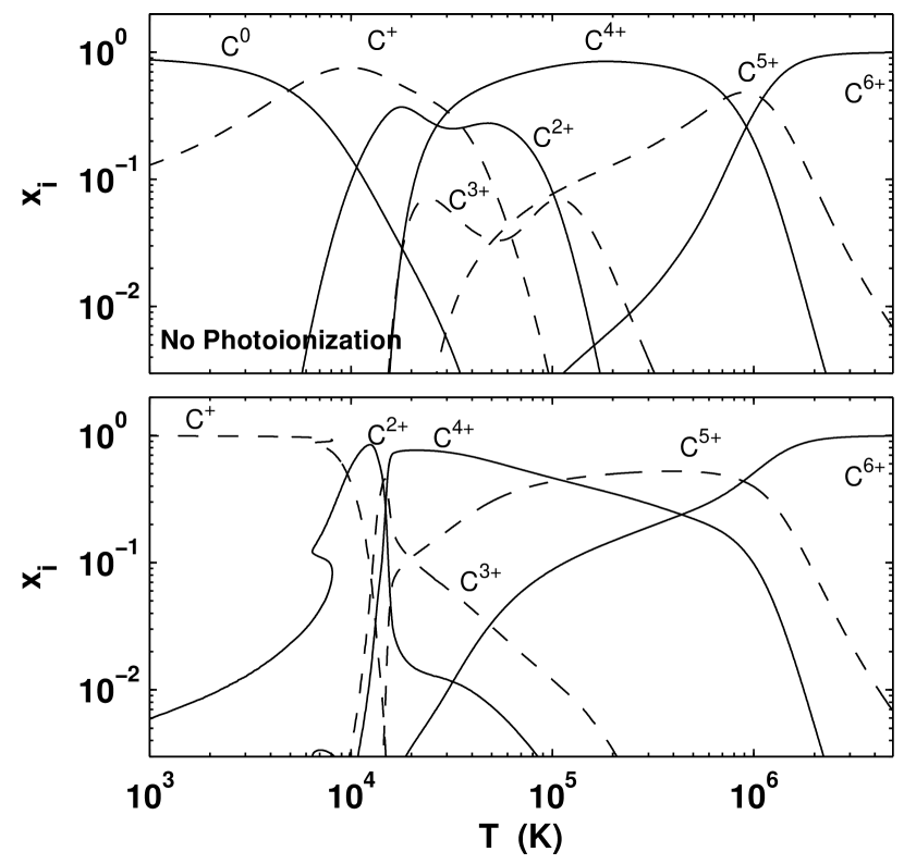
Figure 13.— Carbon ion fractions versus gas temperature in a $T_{s}=5\times 10^{6}$ K strong-$B$ shock for $Z=1$. The upper panel shows a non-physical model in which photoionization is not included in the computation. The lower panel shows results when photoionization is included.

In the hottest parts of the flow where $T\gtrsim 10^{6}$ K, the ionizing radiation has a negligible effect on the ion fractions, because the typical ionization potentials are too high to be efficiently affected by the radiation. At lower temperatures, photoionization becomes important. For example, in the post-shock gas the C⁵⁺ ion fraction remains higher than $10\%$ down to a temperature of $\sim 2\times 10^{4}$ K, whereas without photoionization it drops below $10\%$ at $T\sim 10^{5}$ K. As expected, photoionization becomes dominant at lower temperatures, maintaining C²⁺ as an abundant species below $10^{4}$ K, and C⁺ the most abundant species even at $T\sim 10^{3}$ K. Without radiation, the ionization level is much lower, and neutral carbon is the most dominant species below $5000$ K. Photoionization thus strongly affects the resulting integrated column densities in the cooling layer. The column density of the high-ion C⁵⁺ is enhanced by a factor of $\sim 1.5$ due to photoionization. The column densities of the mid- and low-ions C³⁺, C²⁺, and C⁺ are enhanced by factors of more than $100$.

4.2. Shock Temperature

The shock self-radiation depends on the shock velocity and associated initial post-shock temperature $T_{s}$. As discussed in § 3.2 (equation [11]), the mean intensity of the radiation field is proportional to $T_{s}^{1.5}$. In addition to the overall intensity dependence, the spectral-energy distribution hardens with increasing $T_{s}$. Figure 5 shows the spectral energy distributions for $T_{s}$ equal to $5\times 10^{6}$ K and $5\times 10^{7}$ K. Even high ions, which are only collisionally ionized in a $5\times 10^{6}$ K shock, are photoionized by the harder photon emitted in a $5\times 10^{7}$ K shock. The gas in the hotter shock is more highly ionized, both due to the higher intensity, and the harder spectral shape of the shock radiation.

In Figure 14 we show the carbon ion fractions as a function of gas temperature. The upper panel is for $T_{s}=5\times 10^{7}$ K, and the lower panel is for $T_{s}=5\times 10^{6}$ K. It is clear that the gas is more highly ionized for the hotter shock. This is evident even at very high temperatures, $>10^{6}$ K, where the more energetic photons created by the hotter bremsstrahlung continuum of the $5\times 10^{7}$ K-shock efficiently ionize C⁵⁺ to C⁶⁺.

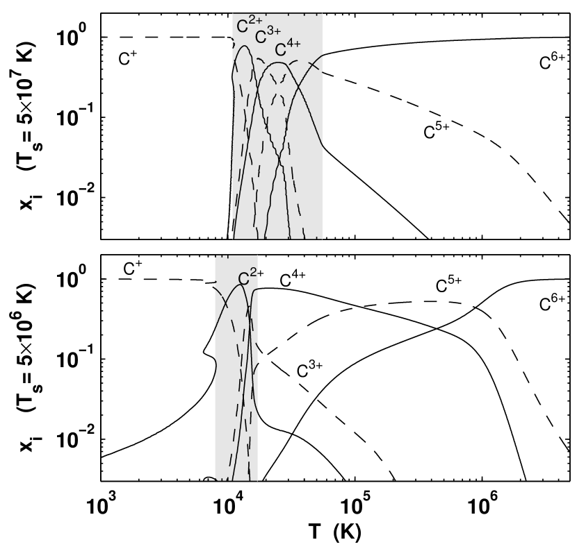
Figure 14.— Carbon ion fraction versus gas temperature in a solar metallicity gas, for a strong-$B$ (isochoric) shock. The upper panel shows results for a shock temperature of $5\times 10^{7}$ K, and the lower panel shows results for $5\times 10^{6}$ K.

Some of the differences between the ion distributions shown in Figure 14 for the two shock velocities, result from the fact that the various “zones” occur at different gas temperatures depending on $T_{s}$. For example, the ranges of temperatures at which the gas is in the WIM plateau (see § 3) are marked in Figure 14 by the gray shaded zones. The WIM plateau starts at a temperature of $\sim 5.5\times 10^{4}$ K for $T_{s}=5\times 10^{7}$ K, and at a temperature of $\sim 1.6\times 10^{4}$ K for $T_{s}=5\times 10^{6}$ K. As the radiation is absorbed in the plateau, the carbon ionization states drops to C³⁺, then C²⁺, and eventually to C⁺ towards the end of the WIM plateau where hydrogen and helium become neutral. While this recombination process takes place within the WIM plateau for both values of $T_{s}$, the ion distributions versus temperature, $x_{i}(T)$, are different.

In the absence of photoionization, the ion fractions, for ions that are produced collisionally at temperatures less than $T_{s}$, are independent of the shock velocity. Thus, without photoionization the ion fractions versus temperature shown in Fig. 17 would be identical for the two shock temperatures. The integrated column densities through the flow are then proportional to the shock velocity (e.g. Heckman et al. 2002). However, as is clearly seen from Figures 13 and 14, photoionization plays a major role in setting the ion fractions in the flow, and the ion distributions are affected by the metallicity, shock temperature, and magnetic field, through their control of the ionization parameter. We present detailed results for the ionic column densities in § 6.

4.3. Magnetic Field

One of the parameters that determines the level of photoionization in the post-shock gas is the strength of the magnetic field. As discussed in § 3.4, the magnetic field strongly affects the ionization parameter in the downstream gas, due to the compression that takes place when $B$ is small. We therefore expect that at low temperatures, after significant compression has taken place, models with $B=0$ will be much less ionized than strong-$B$ isochoric models.

Figure 15 shows the carbon ion fractions in the isobaric $B=0$ (upper panel), and isochoric strong-B (lower panel) limits. The lower ionization parameter in the downstream gas when $B=0$ results in lower ionization states at all temperatures. For example, at a temperature of $30,000$ K, $>98\%$ of the carbon is in the state of C³⁺-C⁵⁺ in the limit of strong-$B$, whereas for $B=0$ more than half of the carbon is in the state of C⁰-C²⁺.

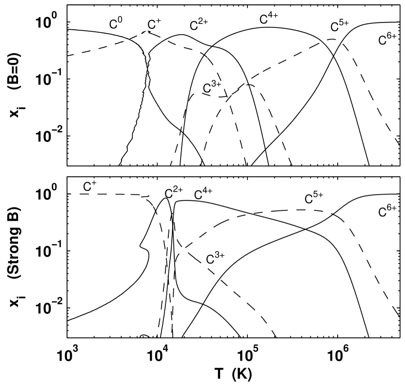
Figure 15.— Carbon ion fractions versus gas temperature in a $T_{s}=5\times 10^{6}$ K shock for $Z=0$. The upper panel is for $B=0$, and the lower panel is for strong-$B$.

For $B=0$, the temperature versus time in the post-shock cooling layers depends on the density, at temperatures lower than $\sim 10^{4}$ K (see § 3.5) where collisional de-excitations of fine-structure transitions become significant. The physical conditions below $T\sim 10^{4}$ K, therefore depend on the density of the shocked medium. The computations presented here assume a post-shock hydrogen density of $0.1$ cm^-3.

4.4. Departures from Equilibrium Ionization

In a photoionized gas with a high ionization parameter, the ion fractions depend only weakly on the gas temperature, as opposed to purely collisionally ionized gas. Since the gas does not have to significantly adjust its ionization state to the time-dependent temperature during cooling, departures from equilibrium are expected to be smaller than for pure radiative cooling.

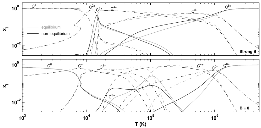
Figure 16.— Carbon ion fractions versus gas temperature in $T_{s}=5\times 10^{6}$ K shocks, for a solar metallicity gas. The upper panel is for the strong-$B$ limit, and the lower panel is for $B=0$. The gray curves show the local photoionization equilibrium ion fractions.

To demonstrate how departures from equilibrium affect the ion fractions, we compare our time-dependent models to a computation in which local equilibrium ionization is imposed everywhere, given the local mean intensities and temperatures that obtain for $5\times 10^{6}$ K, $Z=1$ shocks. In the comparison calculations we use the mean intensities and temperatures derived from the full time-dependent computations. (These mean intensities are different from those that would be derived in a “self-consistent” equilibrium model.) Figure 16 shows the time-dependent (dark) and equilibrium (gray) carbon ion fractions as a function of temperature. The upper panel is for a strong-$B$ isochoric model, and the lower panel is for $B=0$.

For strong-$B$ shocks, the upper of Figure 16 shows that departures from photoionization equilibrium occur at temperatures between $\sim 2\times 10^{4}$ K and $\sim 10^{6}$ K, but the ion fractions differ by $\lesssim 25\%$. These differences are significantly smaller than the differences in the absence of photoionization (GS07). In strong-$B$ shocks, photoionization increases the abundances of high-ions at low temperatures, beyond the enhancement of the “collisional” recombination lag (see Figure 13). The time-dependent ionization states then remain close to photoionization equilibrium (to within $25\%$) even in the non-equilibrium cooling zone.

The lower panel shows that when $B=0$, departures from equilibrium ionization are larger, due to the smaller effect of photoionization resulting from the gas compression (see § 4.3). For example, the non-equilibrium abundance of C⁴⁺ is greater than $0.05$ down to $\sim 2.2\times 10^{4}$ K, whereas the equilibrium abundance vanishes below $\sim 3.3\times 10^{4}$ K. Departures from equilibrium ionization tend to keep the gas at any temperature over-ionized, as recombination lags behind cooling. The contribution of photoionization increases the equilibrium ion fractions relative to the case of pure radiative cooling (GS07), especially at $T\lesssim 10^{5}$K, where the shock self-radiation is energetic enough to efficiently ionize the abundant species, but the compression is still not too large to maintain a significant ionization parameter. At lower temperatures, the non-equilibrium ion-fractions are due entirely to the recombination lags in the collisionally ionized gas. Below $\sim 10^{4}$ K, efficient heating increases the net cooling times significantly, and the gas approaches photoionization equilibrium as can be seen by the near overlap between the dark and gray curves.

4.5. Gas Metallicity

Our results for the non-equilibrium ion fractions, $x_{i}(T)$, for metallicities $Z$ equal to $10^{-3}$, $10^{-2}$, $10^{-1}$, $1$ and $2$, are presented in Table 3. Figure 11 shows, as an example, the carbon ion fractions for the different values of $Z$. The assumed metallicity affects the ion fractions in several ways. First, the cooling times depend on the metal abundance. Higher $Z$ leads to enhanced metal lines cooling, and therefore shorter cooling times. Departures from equilibrium and recombination lags are therefore larger for higher metal abundances. Higher metallicity gas will tend to be more over-ionized.

Second, the spectral shape of the shock self radiation depends on the gas metallicity. Since metal line emission is enhanced for higher $Z$, a larger fraction of the initial energy is radiated via line emission, and a smaller fraction as bremsstrahlung continuum. High-metallicity shocks therefore produce more photons with energies between $1$ and $\sim 5$ Rydbergs, and fewer photons with $E\gtrsim 6$ Rydbergs. At low $Z$ the shock self-radiation is harder. The changing spectral energy distribution as a function of gas metallicity affects the photoionization rates, and therefore the ion fractions as a function of temperature.

As examples illustrating the various effects, in Figure 17a-c we display the C³⁺, O⁵⁺, and Ne⁷⁺ distributions for the different values of $Z$ for a $5\times 10^{6}$ K shock in the strong-B limit. For comparison, in panels (d)-(f) we shows the local equilibrium ion fractions, given the local mean intensities and temperatures that obtain in the shock.

Panel (a) shows that carbon is more over-ionized for higher metallicity gas, and that the C³⁺ ion fraction peaks at lower temperatures for higher $Z$. For example, for $Z=2$ the C³⁺ distribution peaks at $T\simeq 10^{4}$ K. For smaller $Z$, the ion fraction peaks at higher temperatures. For $Z=10^{-3}$, it peaks at $T\simeq 2\times 10^{4}$ K. The sharp decline in the C³⁺ fraction at $\sim 10^{4}$ K, is related to the onset of the photoabsorption plateau, which occurs at a metallicity-dependent temperature (see § 3.2). Panels (a) and (d) show that the C³⁺ fraction remains close to its equilibrium distribution for any value of $Z$, and for the entire temperature range over which it is abundant ($\sim 10^{4}-2\times 10^{5}$ K).

O⁵⁺ shows similar behavior. The higher metallicity shocks are more over-ionized, and the O⁵⁺ fraction persists to lower temperatures where the photoabsorption plateau occurs. A comparison of panels (b) and (e) shows that departures from equilibrium ionization occur only for $Z\gtrsim 1$, and are limited to $T\sim 3\times 10^{5}$ K where the role of photoionization is still minor.

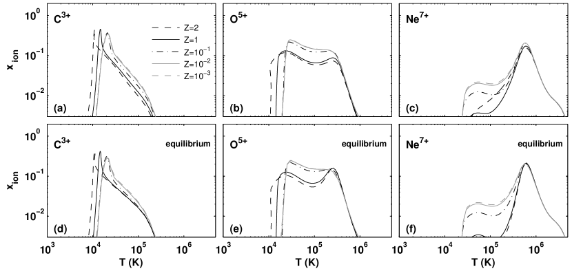
Figure 17.— C³⁺, O⁵⁺, and Ne⁷⁺ ion fraction versus temperature for gas metallicities between $10^{-3}$ and $2$ times solar, in a $5\times 10^{6}$ K shock in the limit of strong-$B$ (panels [a]-[c]). Panels (d)-(f) show, for comparison, the local equilibrium ion fractions, given the local mean intensities and temperatures that obtain in the shock.

For Ne⁷⁺, the behavior is a bit more complicated. At high gas metallicities ($Z>1$), the recombination lags enhance the Ne⁷⁺ abundances above the enhancements due to photoionization, for temperatures between $4\times 10^{4}$ and $2\times 10^{5}$ K. Because the spectral energy distributions for $Z=2$ and for $Z=1$ are similar, the equilibrium distributions are identical. They are also narrower than the non-equilibrium distributions. However, for lower values of $Z$ ($<0.1$), the varying spectral energy distributions affects the Ne⁷⁺ fractions. Figure 2 shows that there are more photons capable of ionizing Ne⁶⁺ (with an ionization threshold of $15.2$ Ryd) for low $Z$, than for $Z=2$. Indeed, for decreasing $Z$ the Ne⁷⁺ ion distribution becomes broader again, due to enhanced photoionization by the shock radiation. This can be seen in panel (f). A comparison with panel (c) then shows that for $Z<0.1$ the Ne⁷⁺-fraction approaches the equilibrium distribution controlled by photoionization.

At low gas metallicities ($\lesssim 10^{-2}$), the total contributions of the metals to the gas cooling and to the emissivity becomes negligible (GS07). The cooling rates and spectral energy distributions therefore become independent of $Z$. This can be clearly seen in Figure 17, where the ion distributions for $Z=10^{-2}$ and for $Z=10^{-3}$ are similar for C³⁺, O⁵⁺, and Ne⁷⁺.

4.6. Auger Effects

We have included multi-electron Auger ionizations using cross section and yields from Kaastra & Mewe (1993). Auger ionization is a potential source of multiply charged metal species in largely neutral (and cool) hydrogen gas, due to the large penetration depths of high-energy photons. However, we find that rapid charge-transfer neutralization with atomic hydrogen quickly removes such ions. The metal abundances are therefore not significantly affected by the Auger processes (cf. Dopita and Sutherland 1996). However, the charge transfer reactions do lead to a slight rise in the ionized-hydrogen (proton) densities. We demonstrate this effect in Figure 18 for a strong-$B$, $Z=1$, $5\times 10^{7}$ K shock, in which intense X-rays are produced. The dark and gray solid lines show the ionized hydrogen fractions with and without the inclusion of Auger processes. Major contributors to the increase in the ionized hydrogen fraction are charge-transfer reactions with Fe and Si ions. The dark dashed curve shows the H⁺ abundances if Auger ionizations are included for iron ions only.

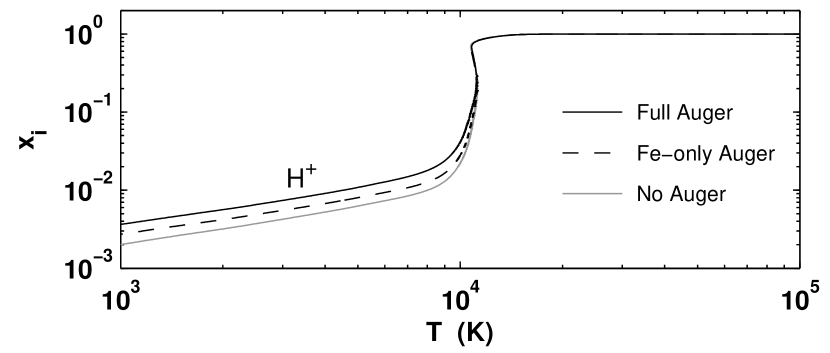
Figure 18.— H⁺ fraction as a function of temperature for a strong-$B$, $5\times 10^{7}$ K shock at $Z=1$. The dark solid line shows the H⁺ fraction when multi-electron Auger ionizations are included. The gray solid line shows a model in which Auger ionizations are excluded. The dashed curve shows the H⁺ ion fraction when Auger ionizations are only included for iron ions.

5. Heating and Cooling

We have carried out computations of the heating and cooling efficiencies in the post-shock cooling layers for shock temperatures of $5\times 10^{6}$ K and $5\times 10^{7}$ K, for gas metallicities $Z$ between $10^{-3}$ and $2$, for $B=0$ and strong-$B$ dynamics. Our results for the heating rates and cooling efficiencies are listed in Table 5, as outlined by Table 4. We use the self-consistent non-equilibrium ion fractions, $x_{i}$, obtained in § 4 to compute $\Lambda(T,x_{i},Z)$ and $\Upsilon(x_{i},Z,J_{\nu})$ for all temperatures in the downstream gas. There is no external source of photoionization and heating, and all of the heating radiation is produced by the shock itself. In all of our shock models, photo-heating is negligible above temperatures of a few $\times 10^{4}$ K and the gas undergoes pure radiative cooling. However, as discussed in § 4, photoionization of the metals can become a very important process even in the hotter components, and this can alter the radiative cooling efficiencies.

Table 5Cooling and Heating in a $5\times 10^{6}$ K, $2$ times solar, strong-$B$-shock

Time	Temperature	$\Lambda$	$\Upsilon$
(s)	(T)	(erg s-1 cm3)	(erg s-1)
$0.00$	$5.000\times 10^{6}$	$2.72\times 10^{-21}$	$2.98\times 10^{-27}$
$7.25\times 10^{8}$	$4.998\times 10^{6}$	$2.34\times 10^{-21}$	$4.38\times 10^{-28}$
$1.57\times 10^{9}$	$4.997\times 10^{6}$	$2.10\times 10^{-21}$	$1.79\times 10^{-28}$

Note. — The complete version of this table is in the electronic edition of the Journal. The printed edition contains only a sample. The full table lists the cooling and heating for strong-$B$ and for $B=0$, for shock temperatures of $5\times 10^{6}$ K and $5\times 10^{7}$ K, and for $Z=10^{-3}$, $10^{-2}$, $10^{-1}$, $1$, and $2$ (for a guide, see Table 4). The times in the first column are given assuming a post-shock hydrogen density of $0.1$ cm^-3. $\Lambda$ and $\Upsilon$ are defined such that the cooling rate per volume is $n_{e}n_{\rm H}\Lambda$, and the heating rate per volume is $n_{\rm tot}\Upsilon$.

For $Z\gtrsim 0.1$, the radiative cooling between a few $\times 10^{4}$ K and $\sim 10^{7}$ K is dominated by electron impact excitation of resonance line transitions of metal ions. Above $\sim 10^{7}$ K, bremsstrahlung cooling dominates for all gas metallicities. At lower temperatures ($\lesssim 10^{4}$ K), Ly$\alpha$ cooling and fine-structure lines dominate the cooling, with relative contributions depending on $T$ and $Z$, as we discuss below (Boehringer & Hensler 1989; Sutherland & Dopita 1996; GS07).

As an example, in Figure 19 we show the cooling and heating rates per unit volume, $n_{e}n_{H}\Lambda$ and $n\Upsilon$, as a function of time (in panel [a]), and as a function of temperature (in panel[ b]) for a strong-$B$, $T_{s}=5\times 10^{6}$ K shock at $Z=1$. In panel (a), we have assumed a post-shock hydrogen density of 0.1 cm^-3 for the cooling time-scales. The dominant cooling and heating elements are indicated near the curves.

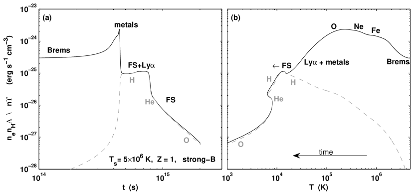
Figure 19.— The cooling (dark) and heating (gray) rates per unit volume (erg s^-1 cm^-3) for a strong-B $5\times 10^{6}$ K at $Z=1$. (a) Cooling and heating rates per unit volume as a function of time, assuming a post-shock hydrogen density $n_{0}=0.1$ cm^-3. (b) Cooling and heating rates per unit volume as a function of temperature. The dominant cooling and heating elements are indicated near the curves.

The gas starts out in the “hot radiative” phase. In this model it remains in this phase for $\sim 3.5\times 10^{14}$ s, and cools gradually, via metal resonance transitions and bremsstrahlung emission, down to a temperature of $\sim 2.5\times 10^{6}$ K. It then enters the “non-equilibrium cooling” phase, where it rapidly cools to a temperature of $\sim 10^{4}$ K via very efficient metal line cooling. This cooling is due mainly to iron, neon, and oxygen ions, as indicated in Figure 19b. Throughout the “hot radiative” and “non-equilibrium cooling” phases, heating is negligible, and the gas cools radiatively from the initial hot shock temperature down to $\sim 10^{4}$ K. However, since photoionization has a major influence on the ion fractions, the non-equilibrium cooling rates differ significantly from those presented in GS07 in which no sources of ionizing radiation were considered. We discuss this point further below.

As discussed in § 3, once the neutral hydrogen fraction becomes large enough, $\gtrsim 10^{-3}$, to allow for efficient photoabsorption, the gas enters the “WIM photoabsorption plateau”. In this stage, heating is mainly due to H and He⁺ photoabsorption. As previously discussed, for $Z=1$, Ly$\alpha$ provides only $15\%$ of the cooling at its peak efficiency. The rest of the cooling is provided by metal resonance lines for $T\gtrsim 2\times 10^{4}$ K, and by fine-structure (FS) and resonance line transitions at lower temperatures. For lower gas metallicities, Ly$\alpha$ constitutes a larger fraction of the cooling at $T\sim 10^{4}$ K. Below $\lesssim 8000$ K, Ly$\alpha$ cooling vanishes and the cooling is dominated entirely by fine-structure transitions.

Heating is first dominated by hydrogen photoabsorption. As the radiation is increasingly absorbed and the gas cools to $\sim 6500$ K, helium photoabsorption dominates the heating. Finally, below $\sim 2000$ K, and as the ionizing radiation becomes even harder, oxygen and other metals become significant absorbers. In the WIM and WNM plateaus the gas remains close to thermal equilibrium, as is evident by the fact that the heating and cooling curves nearly overlap. The delicate balance between heating and cooling that depends on the temperature, electron density and ion fractions, determines the temperatures profiles that were discussed in § 3.

The way in which the cooling efficiency, $\Lambda$, depends on the gas metallicity determines the column-density ratios in the post-shock cooling layers, as we discuss in § 6 below. For $T>10^{7}$ K, cooling is dominated by bremsstrahlung emission for all gas metallicities, and the cooling efficiency is therefore only weakly dependent on $Z$.

For $2\times 10^{4}$ K$~{}\lesssim T\lesssim 10^{7}$ K, resonance metal line transitions are efficiently excited. For $Z\gtrsim 0.1$, the dominant cooling process is metal line cooling, and $\Lambda\propto 1/Z$. For $Z\lesssim 0.01$, the contribution of metals to the gas cooling is negligible. The cooling is dominated by bremsstrahlung emission and by hydrogen and helium Ly$\alpha$, and $\Lambda$ is therefore independent of $Z$.

At $T\sim 10^{4}$ K, a mixture of metal fine structure and Ly$\alpha$ emissions provide the gas cooling. For isochoric flows with $Z>1$, fine-structure emissions dominate the cooling, and $\Lambda$ is therefore proportional to $1/Z$. For lower gas metallicities, and in $B=0$ flows Ly$\alpha$ emission dominates the cooling and $\Lambda$ is independent of $Z$.

Below $\sim 7000$ K, fine structure line emissions are the only available coolants we have included and $\Lambda$ is therefore proportional to $Z$ for all gas metallicities. The dependence of $\Lambda$ on $Z$ is summarized in Table 6 below. These scalings will be useful in § 6.

Table 6The Dependence of $\Lambda(x_{i},T)$ on $Z$

Temperature	Cooling efficiency, $\Lambda(x_{i},T)$
K	$Z\lesssim 10^{-2}$	$10^{-2}<Z<1$	$Z\gtrsim 1$
$\lesssim 7000$	$\propto Z$ (1)	$\propto Z$ (1)	$\propto Z$ (1)
$\sim 10^{4}$	$\propto 1$ (2)	$\propto 1$ (2)	$\propto Z$ (1)
$2\times 10^{4}-10^{7}$	$\propto 1$ (3)	$\propto Z$ (4)	$\propto Z$ (4)
$\gtrsim 10^{7}$	$\propto 1$ (5)	$\propto 1$ (5)	$\propto 1$ (5)

Note. — Given a set of ion fractions $x_{i}$, and a temperature $T$, the table shows how the cooling efficiency $\Lambda(x_{i},T)$ depends on the gas metallicity $Z$. The entry “$\propto 1$” means that the cooling efficiency is nearly independent of $Z$ (but does depend on $x_{i}$ and $T$).

(1) FS line cooling.

(2) H Ly$\alpha$ cooling.

(3) H, He, and bremsstrahlung cooling.

(4) Metal resonance line cooling.

(5) Bremsstrahlung cooling.

In Figure 20, we display the cooling efficiencies for $Z$ between $10^{-3}$ and $2$, in the “hot radiative” and “non-equilibrium cooling” phases for the $T_{s}=5\times 10^{6}$ K (left panels) and $T_{s}=5\times 10^{7}$ K (right panels) shocks that we have considered, in the $B=0$ (lower panels) and strong-B limits (upper panels). We display results for temperatures between $5\times 10^{6}$ K, and the temperatures at which the photoabsorption plateau begins.

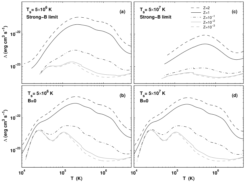
Figure 20.— The cooling efficiencies, $\Lambda$ (erg cm³ s^-1), as a function of temperature in the “hot radiative” and “non-equilibrium cooling” zones. Each panel shows results for gas metallicities between $10^{-3}$ and $2$ times solar. For the range of temperatures displayed in this figure, heating is negligible. The curves end where the photoabsorption plateaus begin. (a) $T_{s}=5\times 10^{6}$ K, for strong-$B$. (b) $T_{s}=5\times 10^{6}$ K, for $B=0$. (c) $T_{s}=5\times 10^{7}$ K, for strong-$B$. (d) $T_{s}=5\times 10^{7}$ K, for $B=0$.

Consider first the $5\times 10^{6}$ K shocks. For $B=0$ (isobaric) the gas compression reduces the photoionization parameter, and the non-equilibrium ion-fractions are mostly due to the recombination lags in the collisionally ionized gas. In this limit, therefore, the cooling curves are almost identical to the non-equilibrium cooling curves presented in GS07 in which photoionization processes were excluded. However, as discussed in § 4, in the strong-B (isochoric) limit, photoionization by the shock radiation significantly increases the ionization state of the gas above the non-equilibrium level that obtains in a purely radiatively cooling gas. More highly ionized species generally have more energetic resonance line transitions, and these are less efficiently excited by the thermal electrons at any given temperature (McCray 1987). The cooling curves are therefore suppressed, compared to $B=0$ shocks.

For the hotter $5\times 10^{7}$ K shock, the shock radiation is more intense, and photoionization drives the ion fractions to still higher ionization states. Again, the more highly ionized gas cools less efficiently, and the cooling rates at a given temperature are therefore lower compared to the $5\times 10^{6}$ K shocks. In the strong-$B$ limit the intensity of the radiation is high enough that even minute amounts of neutral hydrogen allow for efficient photoabsorption heating, and the photoabsorption plateaus begin at a higher temperature of $\sim 5\times 10^{4}$ K.

6. Cooling Columns in Shocked Gas

In this section we present computations of the integrated metal-ion column densities that are produced in the post-shock cooling layers. In computing the cooling columns, we integrate from the shock front to a distance where the gas has cooled down to our termination temperature $T_{\rm low}=1000$ K.

As an example of what these integrations look like, in Figure 21 we display the O⁵⁺ ion fraction and accumulated column density, in a strong-$B$, $5\times 10^{6}$ K shock, for $Z=1$. Panel (a) shows the O⁵⁺ ion fraction as a function of time, for an assumed post-shock hydrogen density of $0.1$ cm^-3. Initially, the O⁵⁺ abundance peaks as the gas is ionized after passing the shock front. This first peak is short, with a duration of less than $10^{11}$ s. Later on, a second peak is formed as the gas cools behind the shock front. This second peak lasts for $\sim 10^{14}$ s. Panel (b) shows the ion fraction as a function of temperature. The first abundance peak occurs over such a narrow temperature range ($T\sim T_{s}$) that it cannot be resolved in panel (b). The second abundance peak is seen to occur between a temperature of $\sim 10^{6}$ K, and $\sim 10^{4}$ K.

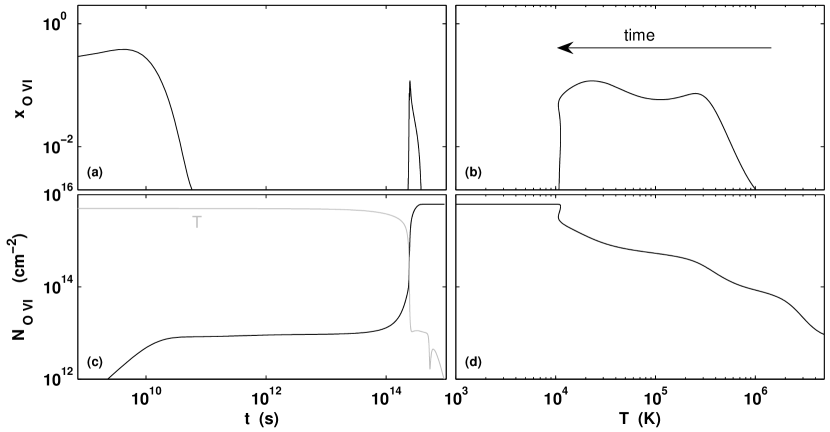
Figure 21.— O⁵⁺ ion fraction (upper panels) and accumulated column density (lower panels) as a function of time (left hand panels) and temperature (right hand panels), for a strong-B, $T_{s}=5\times 10^{6}$ K, $Z=1$ shock. The gray curve in panel (c) shows the temperature (rescaled by $\times 10^{9}$) as a function of time.

Panel (c) shows the accumulated O⁵⁺ column density as a function of time. The initial abundance peak contributes an O⁵⁺ column density of $\sim 10^{13}$ cm^-2. The column density builds rapidly, and remains unchanged until $\gtrsim 10^{14}$ s. The gray curve in panel (c) shows a scaled temperature as a function of time. During the hot radiative phase the accumulated column density remains unaltered, as higher ions dominate the oxygen abundance. The column remains constant until the non-equilibrium cooling phase, during which the second abundance peaks occurs. The column density then builds up rapidly to $\sim 10^{15}$ cm^-2. The O⁵⁺ column keeps increasing in the photoabsorption plateau, until O⁵⁺ finally recombines at $T\sim 10^{4}$ K. The accumulated column density as a function of temperature is shown in panel (d). Panels (c) and (d) show that the contribution of the first abundance peak to the total column density in the post-shock cooling layers is negligible.

More generally, the integrated metal ion column density, $N_{i}$, through the post-shock cooling gas is given by,

$$N_{i}=\int^{0}_{t_{\rm end}}n_{H}ZA_{\rm el}x_{i}vdt\ \ \ ,$$ (12)

with

$$dt\propto\frac{dT}{n\Lambda(x_{i},T,Z)}$$ (13)

In this expression, $n_{H}$ is the hydrogen density, $A_{\rm el}$ is the abundance of the element relative to hydrogen in a solar metallicity gas, $x_{i}$ is the ion fraction, and $v$ is the gas velocity.

Since $n_{H}v$ is constant throughout the flow (eq. [3]), equations (12) and (13) imply that

$$N_{i}\propto Z\int^{T_{s}}_{T_{\rm low}}x_{i}\frac{dT}{n\Lambda}.$$ (14)

For strong-$B$ isochoric flows $n=n_{0}$ everywhere, and $N_{i}\propto Z\int x_{i}dT/\Lambda$. However, for $B=0$ isobaric flows the density increases and the cooling times are shortened as the gas cools (see § 3). Therefore, the column densities of ions produced in low temperature gas are substantially suppressed (by the shorter cooling times) in isobaric versus isochoric cooling flows (e.g. Edgar & Chevalier 1986). For an ion that is produced at a characteristic temperature $T$, the column density in a $B=0$ shock is quenched by a factor approximately $n_{0}/n(T)\simeq T/T_{s}$ relative to a strong-$B$ shock. Because $T/T_{s}$ is smaller for higher $T_{s}$, the quenching effect is more significant for higher shock velocities.

Given an ion distribution $x_{i}(T)$, equation (14) implies that $N_{i}$ is independent of $Z$ if $\Lambda\propto Z$ (as occurs when metals dominate the cooling). When $\Lambda\propto Z$, reduced elemental abundances are compensated by longer cooling times, and $Z$ cancels out in equation (14). On the other hand, for ions that are abundant at temperatures where the cooling is dominated by hydrogen, helium, or bremsstrahlung emissions, equation (14) implies that the column densities are proportional to $Z$.

The actual behavior is more complicated because the ion distributions, $x_{i}(T)$, are themselves a function of gas metallicity and shock temperature as discussed in § 4. For example, higher shock temperatures imply stronger photoionizing radiation fields, which affect the ionization states in the post-shock cooling layers. The gas metallicity affects the spectral energy distribution of the shock self-radiation, changing the ion fractions for different values of $Z$. Departures from equilibrium ionization and the degree of over-ionization in the gas are also a function of gas metallicity. All these factors imply that the column densities depend on the metallicity even for temperatures where $\Lambda\propto Z$.

In Figures 22-25 we display the full set of carbon-, nitrogen, oxygen, and neon-ion column densities, for $Z$ between $10^{-3}$ and $2$, for strong-B (upper panels) and B=0 (lower panels) post-shock cooling layers. Left hand panels are for $T_{s}=5\times 10^{6}$ K, and the right hand panels for $T_{s}=5\times 10^{7}$ K. The shaded areas show ions that are still abundant at $T_{\rm low}=1000$ K. The column densities of these ions (e.g. O and O⁺) are sensitive to the choice of $T_{\rm low}$. The full set of column densities for all the metal ions that we consider are listed in Table 7, as described in Table 4.

Table 7Metal-ion Column Densities in a $5\times 10^{6}$ K, $2$ times solar, strong-$B$-shock

ionization	H	He	C	N	…
	(cm-2)	(cm-2)	(cm-2)	(cm-2)	…
I	$5.7\times 10^{20}$	$4.4\times 10^{19}$	$8.8\times 10^{14}$	$5.7\times 10^{16}$	…
II	$8.5\times 10^{20}$	$2.7\times 10^{19}$	$3.1\times 10^{17}$	$2.3\times 10^{16}$	…
III	–	$4.8\times 10^{19}$	$1.0\times 10^{17}$	$2.2\times 10^{16}$	…

Note. — The complete version of this table is in the electronic edition of the Journal. The printed edition contains only a sample. The full table lists metal-ion column densities for $B=0$ and in the strong-$B$ limit, for shock temperatures of $5\times 10^{6}$ K and $5\times 10^{7}$ K, and for $Z=10^{-3}$, $10^{-2}$, $10^{-1}$, $1$, and $2$ times solar metallicity gas (for a guide, see Table 4).

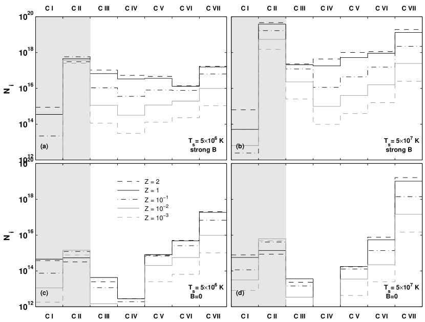
Figure 22.— Carbon ion-column densities in post-shock cooling layers, for $Z$ from $10^{-3}$ to $2$ times solar. (a) $T_{s}=5\times 10^{6}$ K, for strong-$B$. (b) $T_{s}=5\times 10^{7}$ K, for strong-$B$. (c) $T_{s}=5\times 10^{6}$ K, for $B=0$. (d) $T_{s}=5\times 10^{7}$ K, for $B=0$. The shaded areas show ions that are still abundant at $T_{\rm low}=1000$ K where we stop the computation. The column densities of these ions are sensitive to the choice of $T_{\rm low}$.

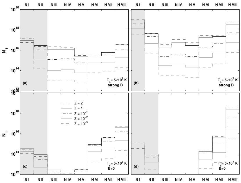
Figure 23.— Same as Figure 22 but for Nitrogen.

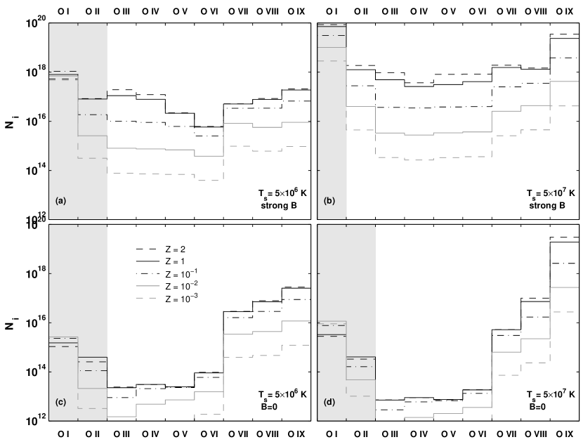
Figure 24.— Same as Figure 22 but for Oxygen.

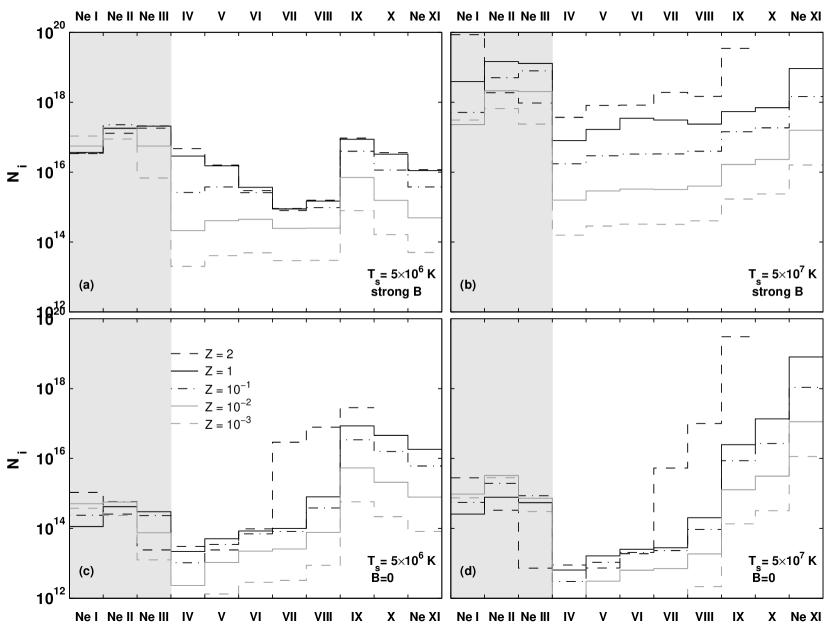
Figure 25.— Same as Figure 22 but for Neon.

Our integrated metal-ion cooling column densities are in good qualitative agreement with the recent results of Allen et al. (2008) for the case of a solar metallicity gas cooling behind a $600$ km s^-1 shock, in which $B\simeq 0$ (their model “J_n1_b0”). Remaining differences are likely due to differences in the assumed elemental abundances, and in the magnetic field strength. The computations presented in Allen et al. cover a different region of the parameter space, and do not show results for the other cases than we consider here (namely $v_{s}=2000$ km s^-1, sub-solar metallicities, and the limit of strong-$B$).

We now focus on the oxygen ion fractions shown in Figure 24 as an example. Table 6 predicts that the column densities in low metallicity gas ($\lesssim 10^{-2}$) are always proportional to $Z$ except at very low temperatures. As can be seen from Figure 24 the ratio between the oxygen ion column densities for $Z=10^{-2}$ and the columns for $Z=10^{-3}$ is $\sim 10$ as expected. For example, in panel (a) the columns of O³⁺, O⁴⁺, and O⁵⁺ are $\sim 8\times 10^{14}$, $\sim 7.5\times 10^{14}$, and $\sim 7\times 10^{14}$ cm^-2 for $Z=10^{-2}$, and $\sim 8\times 10^{13}$, $\sim 7.5\times 10^{14}$, and $\sim 7\times 10^{13}$ for $Z=10^{-3}$. The same applies for other shock temperatures and magnetic field limits, as can be seen in panels (b)-(d).

For $Z>1$, Table 6 predicts that for a given ion distribution $x_{i}$, the column densities are independent of $Z$. Figures 24c and 24d show that for $B=0$ where photoionization is less significant, the column densities for $Z=1$ and for $Z=2$ are indeed similar. Departures from equilibrium have only a very minor impact on the column densities. For example, in Figure 24c, the O⁵⁺ column is $9.6\times 10^{13}$ cm^-2 for $Z=2$, and $9.1\times 10^{13}$ cm^-2 for $Z=1$, due to the longer recombination lags for higher $Z$. However, in strong-$B$ isochoric shocks, photoionization introduces a $Z$ dependence. For example, Figure 24b shows that the O³⁺ column density is $8.1\times 10^{17}$ cm^-2 for $Z=2$, but is $3.1\times 10^{17}$ cm^-2 for $Z=1$. Although $\Lambda\sim Z$, the O³⁺ column density ratio of $2.6$ is in this case even larger than the metallicity-ratio of $2.0$.

Figures 22-25 clearly show the differences between strong-$B$ (isochoric) shocks and $B=0$ (approximately isobaric) shocks. For $B=0$, the gas compression and shorter cooling times reduce the column densities of low and intermediate ions that are formed at $T<T_{s}$. A comparison of Figures 24a and 24c shows that while the column densities of the high ions (O⁶⁺, O⁷⁺) is similar in both cases, the column densities of O²⁺-O⁵⁺ are greatly suppressed in $B=0$ models. For example, in solar metallicity gas, the O⁶⁺ column is, as expected, similar for the two cases. It is $5\times 10^{16}$ cm^-2 for a strong-$B$ shock, and $3\times 10^{16}$ cm^-2 for $B=0$. However, for O³⁺ the column density is $8\times 10^{16}$ cm^-2 for strong-$B$, and $3\times 10^{13}$ cm^-2 for $B=0$, $3.5$ orders of magnitude lower. The magnetic field therefore has a very strong impact on the column density ratios between high- and intermediate-ions, and X-ray and UV observations will be able to easily distinguish between the cases of strong versus weak magnetic fields.

The shock velocity affects the column densities profoundly. Equation 12 implies that for ions that only exist below $T_{s}$, and given an ion distribution $x_{i}(T)$, the integrated column density will be proportional to the shock velocity. However, since the shock self-radiation and the degree of photoionization in the gas depends on the shock temperature, this scaling is not exact. For $B=0$, photoionization is less important, and the ion distributions $x_{i}(T)$ are therefore less sensitive to $T_{s}$. For strong-$B$ shocks, photoionization plays a major role in setting the ion fractions in the cooling gas, and the ion distributions are more affected by $T_{s}$.

For example, panels (a) and (b) show that the column density of O⁴⁺ is $8.1\times 10^{17}$ cm^-2 in a $5\times 10^{7}$ K shock of a two solar metallicity gas, compared to $2.2\times 10^{16}$ cm^-2 in a $5\times 10^{6}$ K shock. This is a factor of $\sim 37$ in the column density, compared to a factor of $10^{1/2}\sim 3$ in the shock velocities. For $B=0$ an additional factor $T/T_{s}$ suppresses the ion column densities as discussed above, and the exact range of temperatures over which the ion is abundant will determine the column density ratio.

7. Metal Columns in the Radiative Precursor

In this section we present equilibrium photoionization computations of the integrated metal-ion column densities that are produced in the radiative precursors. The precursor gas is heated and photoionized by the shock self-radiation propagating upstream. The upstream radiation is gradually absorbed in the radiative precursor, producing a photoabsorption layer in which the heating and ionization rates gradually decline with (upstream) distance from the shock front.

The ionization parameter in the radiative precursor is higher than in the post-shock photoabsorption plateau, because the gas density in the precursor is four times lower than the post-shock density (see § 2.2). Typically, the temperature of the gas approaching the shock front is a few times $10^{4}$ K, but it may be as high as $\sim 10^{5}$ K for $T_{s}=5\times 10^{7}$ K. In computing the precursor columns, we integrate from the shock front to a distance where the heating rate in the unshocked gas is sufficiently low that is reaches a temperature $T_{\rm low}=1000$ K.

We use Cloudy to construct equilibrium photoionization models for the radiative precursors. For the radiation flux entering the precursor, we use the post-shock flux at the position in which the post-shocked gas first becomes thick at the Lyman limit, $l_{thick}$, similarly to the scheme presented in § 2.5. For each shock model, we construct a precursor model assuming that a flux $F_{\nu}(l_{thick})$ enters a gas of density $n_{0}/4$. The metal column densities are then $N_{i}=\int n_{\rm H}ZA_{\rm el}x_{i}dl$, where $l$ is the upstream distance from the shock front, and $n_{\rm H}=n_{0}/4$. In all cases, the precursors are assumed to have a constant density.

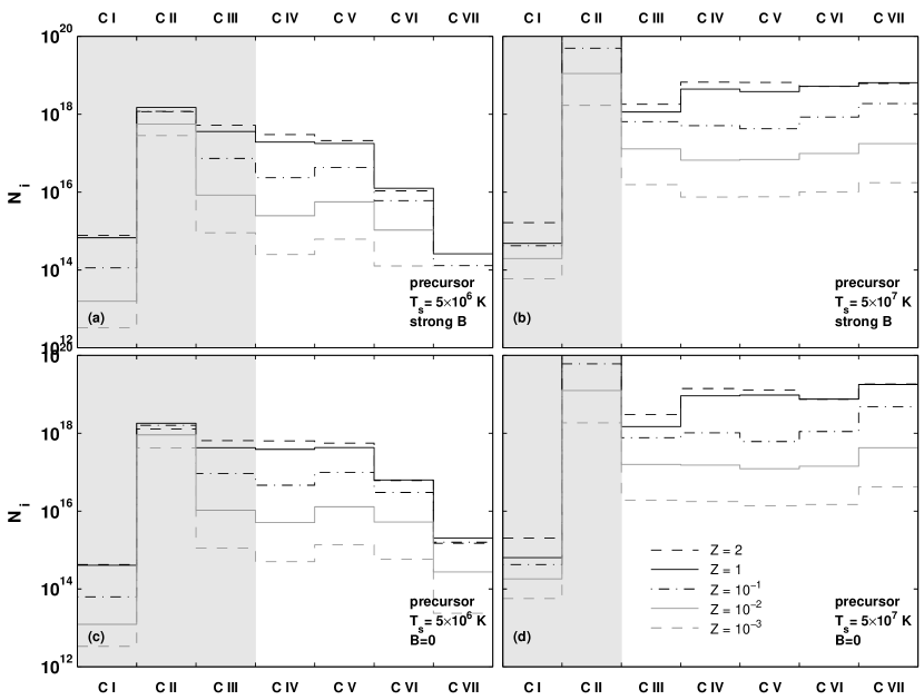
Figure 26.— Carbon ion-column densities in radiative precursor, for $Z$ from $10^{-3}$ to $2$ times solar. (a) $T_{s}=5\times 10^{6}$ K, for strong-$B$. (b) $T_{s}=5\times 10^{7}$ K, for strong-$B$. (c) $T_{s}=5\times 10^{6}$ K, for $B=0$. (d) $T_{s}=5\times 10^{7}$ K, for $B=0$. The shaded areas show ions that are still abundant at $T_{\rm low}=1000$ K where we stop the integration. The column densities of these ions are sensitive to the choice of $T_{\rm low}$.

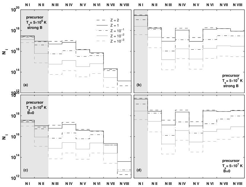
Figure 27.— Same as Figure 22 but for Nitrogen.

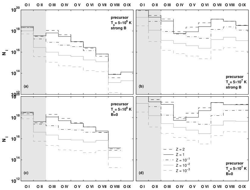
Figure 28.— Same as Figure 22 but for Oxygen.

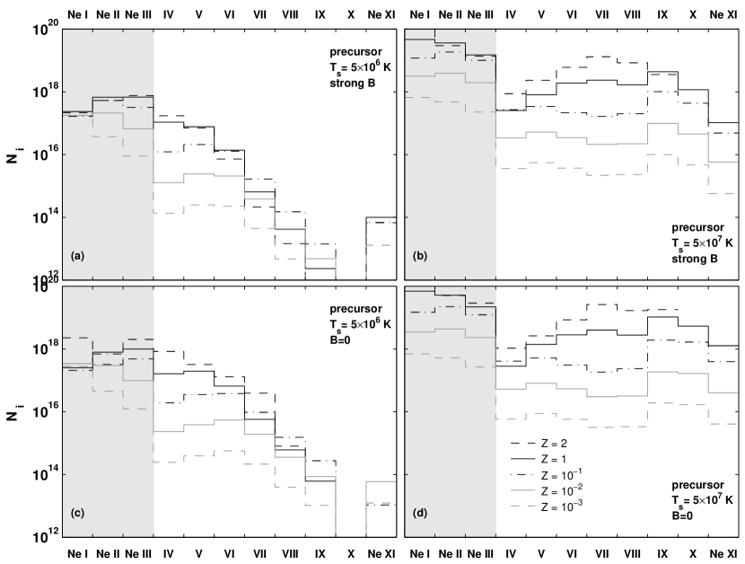
Figure 29.— Same as Figure 22 but for Neon.

Figures 26-29 display the full set of carbon-, nitrogen-, oxygen-, and neon-ion column densities, for $Z$ between $10^{-3}$ and $2$, for the radiative precursors of strong-$B$ (upper panels) and $B=0$ (lower panels) shocks. Left hand panels are for $T_{s}=5\times 10^{6}$ K, and right hand panels are for $T_{s}=5\times 10^{7}$ K. The shaded areas show ions that are still abundant at $T_{\rm low}=1000$ K. The column densities of these ions (e.g. O and O⁺) are sensitive to the choice of $T_{\rm low}$. The full set of column densities for all the metal ions that we consider are listed in Table 8, as described in Table 4. Our integrated precursor column densities are in good qualitative agreement with the recent results of Allen et al. (2008) for the case of a solar metallicity gas cooling behind a $600$ km s^-1 shock, in which $B\simeq 0$ (their model “J_n1_b0”).

Table 8Precursor Column Densities in a $5\times 10^{6}$ K, $2$ times solar, strong-$B$-shock

ionization	H	He	C	N	…
	(cm-2)	(cm-2)	(cm-2)	(cm-2)	…
I	$2.2\times 10^{21}$	$1.7\times 10^{20}$	$7.8\times 10^{14}$	$2.4\times 10^{17}$	…
II	$2.3\times 10^{21}$	$1.5\times 10^{20}$	$1.2\times 10^{18}$	$8.4\times 10^{16}$	…
III	–	$5.5\times 10^{19}$	$5.2\times 10^{17}$	$9.1\times 10^{16}$	…

Note. — The complete version of this table is in the electronic edition of the Journal. The printed edition contains only a sample. The full table lists precursorn column densities for $B=0$ and in the strong-$B$ limit, for shock temperatures of $5\times 10^{6}$ K and $5\times 10^{7}$ K, and for $Z=10^{-3}$, $10^{-2}$, $10^{-1}$, $1$, and $2$ times solar metallicity gas (for a guide, see Table 4).

Figures 26-29 show that significant column densities are created in the radiative precursors. For the high-ions, which collisional abundance peak at $T\sim T_{s}$, the column densities are dominated by the post-shock cooling layers. However, the higher ionization parameters in the lower density precursors allow for a very efficient production of lower ions that are created below $T_{s}$. The precursor columns often exceed the post-shock cooling columns, especially for ions that are maintained by photoionization in the post-shock gas. For example, in solar metallicity gas, the ratio of post-shock to precursor column density of the high ion O VIII, is $N_{\rm post}/N_{\rm pre}=1000$ for a $T_{s}=5\times 10^{6}$ K strong-$B$ shock. The O VIII column is completely dominated by the post-shock gas. However, for O IV this ratio is $0.25$, so that most of the O IV column is created in the precursor.

Higher shocks velocities produce harder and more intense radiation-fields, resulting in efficient production of high-ions and in deeper, higher column-densities, radiative precursors. For example the upper panels in Figure 28 show that when $Z=1$, the O VIII column is $8.5\times 10^{18}$ cm^-2 for $T_{s}=5\times 10^{7}$ K, but $7.7\times 10^{13}$ cm^-2 for $T_{s}=5\times 10^{6}$ K. The O IV column is $5.9\times 10^{17}$ cm^-2 for $T_{s}=5\times 10^{7}$ K, but $3.1\times 10^{17}$ cm^-2 for $T_{s}=5\times 10^{6}$ K.

The column densities produced in the radiative precursors of strong-$B$ shocks are similar to those produced in $B=0$ precursor. The radiative fluxes in the two cases differ only by a factor $5/3$ (see Figure 7). A comparison of the upper and lower panels in Figures 26-29 shows that the precursor columns are indeed similar.

For a given radiation field and absorption depth, the metal-ion column densities scale linearly with gas metallicity. However, since both the spectral energy distribution and the gas opacities are functions of the gas metallicity, some deviations from this linear correlation are expected. For example, lower-$Z$ shocks produce harder radiation fields, which are more efficient in producing high ions. Figures 26-29 shows that the metal-ion column densities generally scale with gas metallicity, but departures from exact linear correlation are apparent in some cases.

While the column densities in the radiative precursor may far exceed the columns produced in the post-shock cooling layers, kinematic differences may distinguish the two components. For high-ions created at $\sim T_{s}$, the kinematic offset between the radiative precursor and the post-shocked gas is $3v_{s}/4$, which is of order the thermal width. Ions produced at lower temperatures have narrower widths, making it possible to distinguish the precursor and post-shock components. In $B=0$ shocks, the post-shock low-ion columns are greatly suppressed (see § 6), and are orders of magnitudes lower than the precursor columns. In strong-$B$ isochoric shocks, significant post-shock low-ion columns are expected to form with a velocity offset of $3v_{s}/4$ relative to the precursor, and with the same velocity centroid as the post-shock high-ions.

8. Summary

In this paper we present new computations of the metal-ion column-densities produced in post-shock cooling layers behind fast, radiative shocks. We have constructed a new (one-dimensional, steady) shock code in which we explicitly follow the non-equilibrium ionization states of post-shock gas containing H, He, C, N, O, Ne, Mg, Si, S, and Fe. We present results for initial post-shock temperatures, $T_{s}$, of $5\times 10^{6}$ and $5\times 10^{7}$ K, corresponding to shock velocities, $v_{s}$, of $600$ and $\sim 2000$ km s^-1. We consider shocks in which there is no magnetic field ($B=0$) for which the cooling flows are approximately isobaric ($P_{\infty}=(4/3)P_{0}$). We also consider shocks in which the magnetic field dominates the pressure everywhere (”strong-$B$”) for which the flows are isochoric ($n_{\infty}=n_{0}$). We assume that the gas is dust free, and we present results for metallicities $Z$ ranging from $10^{-3}$ to twice the solar photospheric abundances of the heavy elements.

For the shock temperatures that we consider, the post-shock gas emits energetic radiation that may later be absorbed by cooler gas further downstream, and by the unperturbed gas that is approaching the shock front. The shock self-radiation significantly affects the ionization states and thermal properties of the gas. Its absorption by the downstream gas creates a photoabsorption zone, in which the temperature and ionization states of the gas are set by the shock self-radiation.

In following the time-dependent ion fractions, we rely on the code and work presented in Gnat & Sternberg (2007). In this paper, in addition to calculating the non-equilibrium ionization and cooling, we also follow the radiative transfer of the shock self-radiation through the post-shock cooling layers; take into account the resulting photoionization and heating rates; follow the dynamics of the cooling gas; and self-consistently compute the initial photoionization states in the precursor gas. We use up-to-date rate coefficients for all of the atomic ionization and recombination processes, and for the energy loss and absorption mechanisms. The equations and our numerical method are presented in § 2.

In § 3 we discuss the shock structure and emitted radiation, and we discuss how these quantities depend on the controlling parameters, including the gas metallicity, shock velocity, magnetic field and gas density (see, e.g. Fig. 1). For $B=0$ shocks (nearly isobaric) the gas is compressed and decelerated as it cools. Because the cooling time-scale is proportional to $1/n$, the final evolutionary stages of isobaric shocks occur much more rapidly than in ”strong-$B$” isochoric shocks. The effects of photoionization by the shock radiation are much more important in isochoric shocks because the ionization parameter remains large in the downstream absorbing layers.

The evolution of the post-shock cooling layers is significantly affected by the gas metallicity in several ways. High metallicity shocks cool more rapidly, because for $10^{4}\lesssim T\lesssim 10^{7}$ K the cooling efficiency is dominated by metal-line cooling. The degree to which recombination lags behind cooling, and the resulting departures from ionization equilibrium therefore depend on the gas metallicity. Second, while the total energy emitted by the cooling gas is independent of $Z$, and equals the energy flux entering the shock, the spectral energy distribution of the shock self-radiation is a function of gas metallicity. For high-$Z$, a high fraction of the input energy is radiated as line-emission, while for low-$Z$, the relative contribution of lines is small, and most of the initial energy flux is radiated as thermal bremsstrahlung continuum. At low $Z$ the shock self-radiation is harder. The photoionization states of the downstream layers depend on the metallicity-dependent spectral energy distributions.

In § 4 we present our computations of the non-equilibrium ionization states in the post-shock cooling layers. In Table 3 we list the time-dependent ion fractions as a function of time and temperature for the various shock models that we consider. As the gas enters the shock, its ionization state rapidly adjusts toward CIE at the shock temperature. Later the gas gradually cools, recombines, and radiates its thermal energy. We describe how photoionization by the shock self-radiation affects the ion fractions in the cooling gas. We find that in strong-$B$ (isochoric) shocks, photoionization plays a central role in setting the ionization states in the cooling layers, even when the gas is still optically thin. Photoionization increases the abundances of high-ions at low temperatures, above the enhancements due to the recombination lags. In those phases where photoionization dominates, the ionization states remain close to photoionization equilibrium. For $B=0$ (isobaric) shocks, the gas compression significantly suppresses the role of photoionization.

We further demonstrate how departures from ionization equilibrium alter the gas ionization. We find that for strong-$B$ shocks, departures from photoionization equilibrium occur at temperatures between $\sim 2\times 10^{4}$ K and $\sim 10^{6}$ K, but the ion fractions differ by $\lesssim 25\%$. However, when $B=0$, departures from equilibrium ionization are larger due to the smaller effect of photoionization, and the non-equilibrium ion-fractions are mostly due to the recombination lags in collisionally ionized gas. We also study the how the ion distributions depend on the gas metallicity, shock velocity, and magnetic field.

We present our computations of the radiative cooling and heating efficiencies in § 5. We list our results in Table 5 and display them in Figure 20. We discuss the different cooling and heating processes that operate in the various cooling “zones” (or ”phases”) and shown in Figures 1 and 4.

Finally, in § 6 and § 7 we present our results for the integrated metal-ion column-densities. In § 6 we discuss the columns that are produced in the post-shock cooling gas. We give results for gas metallicities between $10^{-3}$ and $2$ times the solar abundances. The computed column densities are listed in Table 7. We show that the cooling column densities created in the post shock cooling layers are strong functions of the magnetic field intensity, shock velocity and gas metallicity. Ionic ratios are useful as diagnostic probes. The predicted column densities show that UV and X-ray absorption-line observations of shocked gas may be used to probe the intensity of magnetic fields in interstellar and intergalactic shocks, and to infer the physical properties of gas in fast radiative shock waves. In § 7 we compute the integrated equilibrium metal-ion column densities produced in the upstream radiative precursors. Our precursor column densities are listed in Table 8. For “low-ions”, the column densities produced in the radiative precursors are often comparable to or greater than the post-shock cooling columns. However, kinematic differences between the precursor and post-shock components may provide a means to distinguish observationally between the two contributions.

References

- (1) Allen, M.G., Groves, B.A., Dopita, M.A., Sutherland, R.S., & Kewly, L.J. 2008, astro-ph/0805.0204
- Asplund et al. (2005) Asplund, M., Grevesse, N., & Sauval, A. J. 2005a, ASP Conf. Ser. 336: Cosmic Abundances as Records of Stellar Evolution and Nucleosynthesis, 336, 25
- Ballantyne et al. (2000) Ballantyne, D. R., Ferland, G. J., & Martin, P. G. 2000, ApJ, 536, 773
- (4) Bertone, S., Schaye, J., & Dolag, K. 2008, Space Science Reviews, in press
- (5) Birnboim, Y., & Dekel, A. 2003, MNRAS, 345, 349
- Binette et al. (1985) Binette, L., Dopita, M. A., & Tuohy, I. R. 1985, ApJ, 297, 476
- Boehringer & Hensler (1989) Boehringer, H., & Hensler, G. 1989, A&A, 215, 147
- (8) Bykov, A.M., Dolag, K., & Durret, F. 2008, Space Science Reviews, 134, 119
- Cen & Ostriker (2006) Cen, R., & Ostriker, J. P. 2006, ApJ, 650, 560
- Cen & Ostriker (1999) Cen, R., & Ostriker, J. P. 1999, ApJ, 514, 1
- Chandrasekhar (1960) Chandrasekhar, S. 1960, New York: Dover, 1960
- Chevalier & Imamura (1982) Chevalier, R. A., & Imamura, J. N. 1982, ApJ, 261, 543
- Chevalier et al. (1980) Chevalier, R. A., Kirshner, R. P., & Raymond, J. C. 1980, ApJ, 235, 186
- Collins et al. (2005) Collins, J. A., Shull, J. M., & Giroux, M. L. 2005, ApJ, 623, 196
- Cox (1972) Cox, D. P. 1972, ApJ, 178, 143
- (16) Daltabuit, E., MacAlpine, G.M., & Cox, D.P. 1978, ApJ, 219, 372
- (17) Danforth, C.W., & Shull, J.M. 2008, ApJ, 679, 194
- Davé et al. (2001) Davé, R., et al. 2001, ApJ, 552, 473
- (19) Dekel, A., et al. 2008, Nature, submitted
- (20) Dopita, M.A., & Sutherland, R.S. 2003, Astrophysics of the Diffuse Universe (Springer, Astronomy and astrophysics library)
- (21) Dopita, M.A., & Sutherland, R.S. 1996, ApJS, 102, 161
- Dopita & Sutherland (1995) Dopita, M. A., & Sutherland, R. S. 1995, ApJ, 455, 468
- Dopita (1978) Dopita, M. A. 1978, ApJS, 37, 117
- Dopita (1977) Dopita, M. A. 1977, ApJS, 33, 437
- Dopita (1976) Dopita, M. A. 1976, ApJ, 209, 395
- Draine & McKee (1993) Draine, B.T., & McKee, C.F. 1993, ARA&A, 31, 373
- Draine (1981) Draine, B. T. 1981, ApJ, 245, 880
- Drake & Testa (2005) Drake, J. J., & Testa, P. 2005, Nature, 436, 525
- Edgar & Chevalier (1986) Edgar, R. J., & Chevalier, R. A. 1986, ApJ, 310, L27
- Fang et al. (2006) Fang, T., Mckee, C. F., Canizares, C. R., & Wolfire, M. 2006, ApJ, 644, 174
- Ferland et al. (1998) Ferland, G. J., Korista, K. T., Verner, D. A., Ferguson, J. W., Kingdon, J. B., & Verner, E. M. 1998, PASP, 110, 761
- Fox et al. (2005) Fox, A. J., Wakker, B. P., Savage, B. D., Tripp, T. M., Sembach, K. R., & Bland-Hawthorn, J. 2005, ApJ, 630, 332
- Furlanetto et al. (2005) Furlanetto, S. R., Phillips, L. A., & Kamionkowski, M. 2005, MNRAS, 359, 295
- (34) Furlanetto, S.R., & Loeb, A. 2004, ApJ, 611, 642
- Gaetz et al. (1988) Gaetz, T. J., Edgar, R. J., & Chevalier, R. A. 1988, ApJ, 329, 927
- (36) Ganguly, R., Cen, R., Fang, T., & Sembach. K. 2008, ApJ, 678, L89
- Ghavamian et al. (2007) Ghavamian, P., Laming, J. M., & Rakowski, C. E. 2007, ApJ, 654, L69
- Ghavamian et al. (2001) Ghavamian, P., Raymond, J., Smith, R. C., & Hartigan, P. 2001, ApJ, 547, 995
- Gnat & Sternberg (2007) Gnat, O., & Sternberg, A. 2007, ApJS, 168, 213
- Heckman et al. (2002) Heckman, T. M., Norman, C. A., Strickland, D. K., & Sembach, K. R. 2002, ApJ, 577, 691
- Heng & McCray (2007) Heng, K., & McCray, R. 2007, ApJ, 654, 923
- Heng et al. (2007) Heng, K., van Adelsberg, M., McCray, R., & Raymond, J. C. 2007, ApJ, 668, 275
- Hindmarsh (1983) Hindmarsh, A. C., 1983, ODEPACK, A Systematized Collection of ODE Solvers, in Scientific Computing, R. S. Stepleman et al. (eds.), North-Holland, Amsterdam, 1983 (vol. 1 of IMACS Transactions on Scientific Computation), pp. 55-64.
- Innes (1992) Innes, D. E. 1992, A&A, 256, 660
- Innes et al. (1987) Innes, D. E., Giddings, J. R., & Falle, S. A. E. G. 1987, MNRAS, 226, 67
- Kaastra & Mewe (1993) Kaastra, J. S., & Mewe, R. 1993, A&AS, 97, 443
- Kafatos (1973) Kafatos, M. 1973, ApJ, 182, 433
- (48) Kang, H.& Shapiro, P.R. 1992, ApJ, 386, 432
- (49) Keres, D., Katz, N., Weinberg, D.H., & Dave, R. 2005, MNRAS, 363, 2
- Kingdon & Ferland (1996) Kingdon, J. B., & Ferland, G. J. 1996, ApJS, 106, 205
- Krolik & Raymond (1985) Krolik, J. H., & Raymond, J. C. 1985, ApJ, 298, 660
- Langer et al. (1981) Langer, S. H., Chanmugam, G., & Shaviv, G. 1981, ApJ, 245, L23
- McKee & Hollenbach (1980) McKee, C. F., & Hollenbach, D. J. 1980, ARA&A, 18, 219
- McCray (1987) McCray, R. 1987, in Spectroscopy of Astrophysical Plasmas, Eds. A. Dalgarno & D. Layzer (Cambridge University Press), p. 255
- Nicastro et al. (2005) Nicastro, F., et al. 2005, Nature, 433, 495
- Ostriker & Silk (1973) Ostriker, J., & Silk, J. 1973, ApJ, 184, L113
- (57) Pittard, J.M., Dobson, M.S., Durisen, R.H., Dyson, J.E., Hartquist, T.W., & O’brien, J.T. 2005, AA, 438, 11
- Rakowski et al. (2008) Rakowski, C. E., Laming, J. M., & Ghavamian, P. 2008, ArXiv e-prints, 805, astro-ph/0805.3084
- (59) Ramachandran, B., & Smith M.D. 2006, MNRAS, 366, 586
- Rasmussen et al. (2006) Rasmussen, A. P., Kahn, S. M., Paerels, F., Willem den Herder, J., Kaastra, J., & de Vries, C. 2006, astro-ph/0604515
- Raymond et al. (2008) Raymond, J. C., Isenberg, P. A., & Laming, J. M. 2008, ArXiv e-prints, 804, arXiv:0804.3808
- Raymond (1979) Raymond, J. C. 1979, ApJS, 39, 1
- Richter et al. (2004) Richter, P., Savage, B. D., Tripp, T. M., & Sembach, K. R. 2004, ApJS, 153, 165
- Savage et al. (2005) Savage, B. D., Lehner, N., Wakker, B. P., Sembach, K. R., & Tripp, T. M. 2005, ApJ, 626, 776
- Schmutzler & Tscharnuter (1993) Schmutzler, T., & Tscharnuter, W. M. 1993, A&A, 273, 318
- Sembach et al. (2004) Sembach, K. R., Tripp, T. M., Savage, B. D., & Richter, P. 2004, ApJS, 155, 351
- Shapiro & Moore (1976) Shapiro, P. R., & Moore, R. T. 1976, ApJ, 207, 460
- Shu (1992) Shu, F. H. 1992, Physics of Astrophysics, Vol. II, by Frank H. Shu. Published by University Science Books, ISBN 0-935702-65-2, 476pp, 1992.
- Shull et al. (2003) Shull, J. M., Tumlinson, J., & Giroux, M. L. 2003, ApJ, 594, L107
- Shull & McKee (1979) Shull, J. M., & McKee, C. F. 1979, ApJ, 227, 131
- Soltan et al. (2005) Soltan, A. M., Freyberg, M. J., & Hasinger, G. 2005, å, 436, 67
- Sutherland et al. (2003) Sutherland, R. S., Bisset, D. K., & Bicknell, G. V. 2003, ApJS, 147, 187
- Sutherland & Dopita (1993) Sutherland, R. S., & Dopita, M. A. 1993, ApJS, 88, 253
- Smith et al. (1996) Smith, R. K., Krzewina, L. G., Cox, D. P., Edgar, R. J., & Miller, W. W. I. 1996, ApJ, 473, 864
- Spitzer (1962) Spitzer, L. 1962, Physics of Fully Ionized Gases, New York: Interscience (2nd edition), 1962,
- (76) Strickland, R. & Blondin, J.M. 1995, ApJ, 449, 727
- Sutherland & Dopita (1993) Sutherland, R. S., & Dopita, M. A. 1993, ApJS, 88, 253
- Toth & Draine (1993) Toth, G., & Draine, B. T. 1993, ApJ, 413, 176
- Tripp et al. (2000) Tripp, T. M., Savage, B. D., & Jenkins, E. B. 2000, ApJ, 534, L1
- Tripp et al. (2006) Tripp, T. M., Aracil, B., Bowen, D. V., & Jenkins, E. B. 2006, ApJ, 643, L77
- Tripp et al. (2007) Tripp, T. M., Sembach, K. R., Bowen, D. V., Savage, B. D., Jenkins, E. B., Lehner, N., & Richter, P. 2007, ArXiv e-prints, 706, arXiv:0706.1214
- (82) Tripp, T.M., Sembach, K.R., Bowen, D.V., Savage, B.D., Jenkins, E.B. Lehner, N., & Richter, P. 2008, ApJS, 177, 39
- (83) Tumilson, J, Shull, J.M., Giroux, M.L., & Stocke, J.T. 2005, ApJ, 620, 95
- Verner et al. (1996) Verner, D. A., Ferland, G. J., Korista, K. T., & Yakovlev, D. G. 1996, ApJ, 465, 487
- Williams et al. (2006) Williams, R. J., Mathur, S., Nicastro, F., & Elvis, M. 2006, ApJ, 642, L95
- Yoshida et al. (2005) Yoshida, N., Furlanetto, S. R., & Hernquist, L. 2005, ApJ, 618, L91