Combinatorics of Tripartite Boundary Connections
for Trees and Dimers

Abstract

A grove is a spanning forest of a planar graph in which every component tree contains at least one of a special subset of vertices on the outer face called nodes. For the natural probability measure on groves, we compute various connection probabilities for the nodes in a random grove. In particular, for “tripartite” pairings of the nodes, the probability can be computed as a Pfaffian in the entries of the Dirichlet-to-Neumann matrix (discrete Hilbert transform) of the graph. These formulas generalize the determinant formulas given by Curtis, Ingerman, and Morrow, and by Fomin, for parallel pairings. These Pfaffian formulas are used to give exact expressions for reconstruction: reconstructing the conductances of a planar graph from boundary measurements. We prove similar theorems for the double-dimer model on bipartite planar graphs.

1 Introduction

In a companion paper [KW06] we studied two probability models on finite planar graphs: groves and the double-dimer model.

1.1 Groves

Given a finite planar graph and a set of vertices on the outer face, referred to as nodes, a grove is a spanning forest in which every component tree contains at least one of the nodes. A grove defines a partition of the nodes: two nodes are in the same part if and only if they are in the same component tree of the grove. See Figure 1.

When the edges of the graph are weighted, one defines a probability measure on groves, where the probability of a grove is proportional to the product of its edge weights. We proved in [KW06] that the connection probabilities—the partition of nodes determined by a random grove—could be computed in terms of certain “boundary” measurements. Explicitly, one can think of the graph as a resistor network in which the edge weights are conductances. Suppose the nodes are numbered in counterclockwise order. The $L$ matrix, or Dirichlet-to-Neumann matrix (also known as the response matrix or discrete Hilbert transform), is then the function $L=(L_{i,j})$ indexed by the nodes, with $Lv$ being the vector of net currents out of the nodes when $v$ is a vector of potentials applied to the nodes (and no current loss occurs at the internal vertices). For any partition $\pi$ of the nodes, the probability that a random grove has partition $\pi$ is

$$\Pr(\pi)=\ddddot{\Pr}(\pi)\Pr(1|2|\cdots|n),$$

where $1|2|\cdots|n$ is the partition which connects no nodes, and $\ddddot{\Pr}(\pi)$ is a polynomial in the entries $L_{i,j}$ with integer coefficients (we think of it as a normalized probability, $\ddddot{\Pr}(\pi)=\Pr(\pi)/\Pr(1|2|\cdots|n)$, hence the notation). In [KW06] we showed how the polynomials $\ddddot{\Pr}(\pi)$ could be constructed explicitly as integer linear combinations of elementary polynomials.

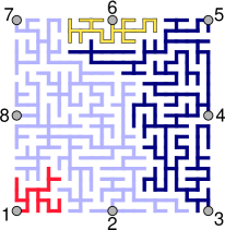
Figure 1: A random grove (left) of a rectangular grid with $8$ nodes on the outer face. In this grove there are $4$ trees (each colored differently), and the partition of the nodes is $\{\{1\},\{2,7,8\},\{3,4,5\},\{6\}\}$, which we write as $1|278|345|6$, and illustrate schematically as shown on the right.

For certain partitions $\pi$, however, there is a simpler formula for $\ddddot{\Pr}(\pi)$: for example, Curtis, Ingerman, and Morrow [CIM98], and Fomin [Fom01], showed that for certain partitions $\pi$, $\ddddot{\Pr}(\pi)$ is a determinant of a submatrix of $L$. We generalize these results in several ways.

Firstly, we give an interpretation (§ 8) of every minor of $L$ in terms of grove probabilities. This is analogous to the all-minors matrix-tree theorem [Cha82] [Che76, pg. 313 Ex. 4.12–4.16, pg. 295], except that the matrix entries are entries of the response matrix rather than edge weights, so in fact the all-minors matrix-tree theorem is a special case.

Secondly, we consider the case of tripartite partitions $\pi$ (see Figure 2), showing that the grove probabilities $\ddddot{\Pr}(\pi)$ can be written as the Pfaffian of an antisymmetric matrix derived from the $L$ matrix. One motivation for studying tripartite partitions is the work of Carroll and Speyer [CS04] and Petersen and Speyer [PS05] on so-called Carroll-Speyer groves (Figure 7) which arose in their study of the cube recurrence. Our tripartite groves directly generalize theirs. See § 9.

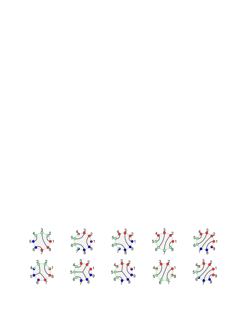
Figure 2: Illustration of tripartite partitions. The two partitions in each column are duals of one another. The nodes come in three colors, red, green, and blue, which are arranged contiguously on the outer face; a node may be split between two colors if it occurs at the transition between these colors. Assuming the number of nodes of each color (where split nodes count as half) satisfies the triangle inequality, there is a unique noncrossing partition with a minimal number of parts in which no part contains nodes of the same color. This partition is called the tripartite partition, and is essentially a pairing, except that there may be singleton nodes (where the colors transition), and there may be a (unique) part of size three. If there is a part of size three, we call the partition a tripod. If one of the color classes is empty (or the triangle inequality is tight), then the partition is the “parallel crossing” studied in [CIM98] and [Fom01].

A third motivation is the conductance reconstruction problem. Under what circumstances does the response matrix ($L$ matrix), which is a function of boundary measurements, determine the conductances on the underlying graph? This question was studied in [CIM98, CdV98, CdVGV96]. Necessary and sufficient conditions are given in [CdVGV96] for two planar graphs on $n$ nodes to have the same response matrix. In [CdV98] it was shown which matrices arise as response matrices of planar graphs. Given a response matrix $L$ satisfying the necessary conditions, in § 7 we use the tripartite grove probabilities to give explicit formulas for the conductances on a standard graph whose response matrix is $L$. This question was first solved in [CIM98], who gave an algorithm for recursively computing the conductances, and was studied further in [CM02, Rus03]. In contrast, our formulas are explicit.

1.2 Double-dimer model

A number of these results extend to another probability model, the double-dimer model on bipartite planar graphs, also discussed in [KW06].

Let $\mathcal{G}$ be a finite bipartite graph embedded in the plane with a set $N$ of $2n$ distinguished vertices (referred to as nodes) which are on the outer face of $\mathcal{G}$ and numbered in counterclockwise order. One can consider a multiset (a subset with multiplicities) of the edges of $\mathcal{G}$ with the property that each vertex except the nodes is the endpoint of exactly two edges, and the nodes are endpoints of exactly one edge in the multiset. In other words, it is a subgraph of degree $2$ at the internal vertices, degree $1$ at the nodes, except for possibly having some doubled edges. Such a configuration is called a double-dimer configuration; it will connect the nodes in pairs.

If edges of $\mathcal{G}$ are weighted with positive real weights, one defines a probability measure in which the probability of a configuration is a constant times the product of weights of its edges (and doubled edges are counted twice), times $2^{\ell}$ where $\ell$ is the number of loops (doubled edges do not count as loops).

We proved in [KW06] that the connection probabilities—the matching of nodes determined by a random configuration—could be computed in terms of certain boundary measurements.

Let $Z^{\mathsf{DD}}(\mathcal{G},\mathbf{N})$ be the weighted sum of all double-dimer configurations. Let $\mathcal{G}^{\mathsf{BW}}$ be the subgraph of $\mathcal{G}$ formed by deleting the nodes except the ones that are black and odd or white and even, and let $\mathcal{G}^{\mathsf{BW}}_{i,j}$ be defined as $\mathcal{G}^{\mathsf{BW}}$ was, but with nodes $i$ and $j$ included in $\mathcal{G}^{\mathsf{BW}}_{i,j}$ if and only if they were not included in $\mathcal{G}^{\mathsf{BW}}$.

A dimer cover, or perfect matching, of a graph is a set of edges whose endpoints cover the vertices exactly once. When the graph has weighted edges, the weight of a dimer configuration is the product of its edge weights. Let $Z^{\mathsf{BW}}$ and $Z^{\mathsf{BW}}_{i,j}$ be the weighted sum of dimer configurations of $\mathcal{G}^{\mathsf{BW}}$ an $\mathcal{G}^{\mathsf{BW}}_{i,j}$, respectively, and define $Z^{\mathsf{WB}}$ and $Z^{\mathsf{WB}}_{i,j}$ similarly but with the roles of black and white reversed. Each of these quantities can be computed via determinants, see [Kas67].

One can easily show that $Z^{\mathsf{DD}}=Z^{\mathsf{BW}}Z^{\mathsf{WB}}$; this is essentially equivalent to Ciucu’s graph factorization theorem [Ciu97]. (The two dimer configurations in Figure 3 are on the graphs $\mathcal{G}^{\mathsf{BW}}$ and $\mathcal{G}^{\mathsf{WB}}$.) The variables that play the role of $L_{i,j}$ in groves are defined by

$$X_{i,j}=Z^{\mathsf{BW}}_{i,j}/Z^{\mathsf{BW}}.$$

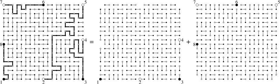
Figure 3: A double-dimer configuration is a union of two dimer configurations.

We showed in [KW06] that for each matching $\pi$, the normalized probability $\widehat{\Pr}(\pi)=\Pr(\pi)Z^{\mathsf{WB}}/Z^{\mathsf{BW}}$ that a random double-dimer configuration connects nodes in the matching $\pi$, is an integer polynomial in the quantities $X_{i,j}$.

In the present paper, we show in Theorem 6.1 that when $\pi$ is a tripartite pairing, that is, the nodes are divided into three consecutive intervals around the boundary and no node is paired with a node in the same interval, $\widehat{\Pr}(\pi)$ is a determinant of a matrix whose entries are the $X_{i,j}$’s or $0$.

1.3 Conductance reconstruction

Recall that an electrical transformation of a resistor network is a local rearrangement of the type shown in Figure 4. These transformations do not change the response matrix of the graph. [CdVGV96] showed that a planar graph with $n$ nodes can be reduced, using electrical transformations, to a standard graph $\Sigma_{n}$ (shown in Figure 5 for $n$ up to $6$), or a minor of one of these graphs (obtained from $\Sigma_{n}$ by deletion/contraction of edges).

\psfrag{=}[bc][Bc][1][0]{$\Leftrightarrow$}\psfrag{a}[bc][Bc][1][0]{$a$}\psfrag{b}[bc][Bc][1][0]{$b$}\psfrag{c}[bc][Bc][1][0]{$c$}\psfrag{a+b}[bc][Bc][1][0]{$a+b$}\psfrag{ab/(a+b)}[bc][Bc][1][0]{\small$ab/(a+b)$}\psfrag{ab/(a+b+c)}[bc][Bc][1][0]{$\frac{ab}{a+b+c}$}\psfrag{ac/(a+b+c)}[bc][Bc][1][0]{$\frac{ac}{a+b+c}$}\psfrag{bc/(a+b+c)}[tc][Bc][1][0]{$\frac{bc}{a+b+c}$}\includegraphics{elec-trans}

Figure 4: Local graph transformations that preserve the electrical response matrix of the graph; the edge weights are the conductances. These transformations also preserve the connection probabilities of random groves, though some of the transformations scale the weighted sum of groves. Any planar graph with $n$ nodes can be transformed to a minor of the “standard graph” $\Sigma_{n}$ (Figure 5) via these transformations [CdVGV96].

\psfrag{G1}[tc][tc][1][0]{$\Sigma_{1}$}\psfrag{G2}[tc][tc][1][0]{$\Sigma_{2}$}\psfrag{G3}[tc][tc][1][0]{$\Sigma_{3}$}\psfrag{G4}[tc][tc][1][0]{$\Sigma_{4}$}\psfrag{G5}[tc][tc][1][0]{$\Sigma_{5}$}\psfrag{G6}[tc][tc][1][0]{$\Sigma_{6}$}\includegraphics{stdgraphs0}

Figure 5: Standard graphs $\Sigma_{n}$ with $n$ nodes for $n$ up to $6$.

In particular the response matrix of any planar graph on $n$ nodes is the same as that for a minor of the standard graph $\Sigma_{n}$ (with certain conductances). [CdV98] computed which matrices occur as response matrices of a planar graph. [CIM98] showed how to reconstruct recursively the edge conductances of $\Sigma_{n}$ from the response matrix, and the reconstruction problem was also studied in [CM02] and [Rus03]. Here we give an explicit formula for the conductances as ratios of Pfaffians of matrices derived from the $L$ matrix and its inverse. These Pfaffians are irreducible polynomials in the matrix entries (Theorem 5.1), so this is in some sense the minimal expression for the conductances in terms of the $L_{i,j}$.

2 Background

Here we collect the relevant facts from [KW06].

2.1 Partitions

We assume that the nodes are labeled $1$ through $n$ counterclockwise around the boundary of the graph $\mathcal{G}$. We denote a partition of the nodes by the sequences of connected nodes, for example $1|234$ denotes the partition consisting of the parts $\{1\}$ and $\{2,3,4\}$, i.e., where nodes $2$, $3$, and $4$ are connected to each other but not to node $1$. A partition is crossing if it contains four items $a<b<c<d$ such that $a$ and $c$ are in the same part, $b$ and $d$ are in the same part, and these two parts are different. A partition is planar if and only if it is non-crossing, that is, it can be represented by arranging the items in order on a circle, and placing a disjoint collection of connected sets in the disk such that items are in the same part of the partition when they are in the same connected set. For example $13|24$ is the only non-planar partition on $4$ nodes.

2.2 Bilinear form and projection matrix

Let $W_{n}$ be the vector space consisting of formal linear combinations of partitions of $\{1,2,\dots,n\}$. Let $U_{n}\subset W_{n}$ be the subspace consisting of formal linear combinations of planar partitions.

On $W_{n}$ we define a bilinear form: if $\tau$ and $\sigma$ are partitions, $\langle\tau,\sigma\rangle_{\mathsf{t}}$ takes value $1$ or $0$ and is equal to $1$ if and only if the following two conditions are satisfied:

1. The number of parts of $\tau$ and $\sigma$ add up to $n+1$.

2. The transitive closure of the relation on the nodes defined by the union of $\tau$ and $\sigma$ has a single equivalence class.

For example $\langle 123|4,24|1|3\rangle_{\mathsf{t}}=1$ but $\langle 12|34,12|3|4\rangle_{\mathsf{t}}=0.$ (We write the subscript $\mathsf{t}$ to distinguish this form from ones that arise in the double-dimer model in § 6.)

This form, restricted to the subspace $U_{n}$, is essentially the “meander matrix”, see [KW06, DFGG97], and has non-zero determinant. Hence the bilinear form is non-degenerate on $U_{n}$. We showed in [KW06], Proposition 2.6, that $W_{n}$ is the direct sum of $U_{n}$ and a subspace $K_{n}$ on which $\langle,\!\rangle_{\mathsf{t}}$ is identically zero. In other words, the rank of $\langle,\!\rangle_{\mathsf{t}}$ is the $n$${}^{\text{th}}$ Catalan number $C_{n}$, which is the dimension of $U_{n}$. Projection to $U_{n}$ along the kernel $K_{n}$ associates to each partition $\tau$ a linear combination of planar partitions. The matrix of this projection is called ${\mathcal{P}}^{(\mathsf{t})}$. It has integer entries [KW06]. Observe that ${\mathcal{P}}^{(\mathsf{t})}$ preserves the number of parts of a partition: each non-planar partition with $k$ parts projects to a linear combination of planar partitions with $k$ parts (this follows from condition 1 above).

2.3 Equivalences

The rows of the projection matrix ${\mathcal{P}}^{(\mathsf{t})}$ determine the crossing probabilities, see Theorem 2.5 below. In this section we give tools for computing columns of ${\mathcal{P}}^{(\mathsf{t})}$.

We say two elements of $W_{n}$ are equivalent ($\stackrel{{\scriptstyle\mathsf{t}}}{{\equiv}}$) if their difference is in $K_{n}$, that is, their inner product with any partition is equal. We have, for example,

Lemma 2.1.

$1|234+2|134+3|124+4|123\stackrel{{\scriptstyle\mathsf{t}}}{{\equiv}}12|34+13|24+14|23$

which is another way of saying that

$${\mathcal{P}}^{(\mathsf{t})}(13|24)=1|234+2|134+3|124+4|123-12|34-14|23.$$

This lemma, together with the following two equivalences, will allow us to write any partition as an equivalent sum of planar partitions. That is, it allows us to compute the columns of ${\mathcal{P}}^{(\mathsf{t})}$.

Lemma 2.2.

Suppose $n\geq 2$, $\tau$ is a partition of $1,\dots,n-1$, and $\tau\stackrel{{\scriptstyle\mathsf{t}}}{{\equiv}}\sum_{\sigma}\alpha_{\sigma}\sigma$. Then

$$\tau|n\stackrel{{\scriptstyle\mathsf{t}}}{{\equiv}}\sum_{\sigma}\alpha_{\sigma}\sigma|n.$$

If $\tau$ is a partition of $1,\dots,n-1$, we can insert $n$ into the part containing item $j$ to get a partition of $1,\dots,n$.

Lemma 2.3.

Suppose $n\geq 2$, $\tau$ is a partition of $1,\dots,n-1$, $1\leq j<n$, and $\tau\stackrel{{\scriptstyle\mathsf{t}}}{{\equiv}}\sum_{\sigma}\alpha_{\sigma}\sigma$. Then

$$\text{\rm[$\tau$ with $n$ inserted into $j$'s part]}\stackrel{{\scriptstyle\mathsf{t}}}{{\equiv}}\sum_{\sigma}\alpha_{\sigma}\text{\rm[$\sigma$ with $n$ inserted into $j$'s part]}.$$

One more lemma is quite useful for computations.

Lemma 2.4 ([KW06, Lemma 4.1]).

If a planar partition $\sigma$ contains only singleton and doubleton parts, and $\sigma^{\prime}$ is the partition obtained from $\sigma$ by deleting all the singleton parts, then the rows of the matrices ${\mathcal{P}}^{(\mathsf{t})}$ for $\sigma$ and $\sigma^{\prime}$ are equal, in the sense that they have the same non-zero entries (when the columns are matched accordingly by deleting the corresponding singletons).

The above lemmas can be used to recursively rewrite a non-planar partition $\tau$ as an equivalent linear combination of planar partitions. As a simple example, to reduce $13|245$, start with the equation from Lemma 2.1 and, using Lemma 2.3, adjoin a $5$ to every part containing $4$, yielding

$$13|245\equiv 1|2345+2|1345+3|1245+45|123-12|345-145|23.$$

2.4 Connection probabilities

For a partition $\tau$ on $1,\dots,n$ we define

$$L_{\tau}=\sum_{F}\prod_{\text{$\{i,j\}\in F$}}L_{i,j},$$ (1)

where the sum is over those spanning forests $F$ of the complete graph on $n$ vertices $1,\dots,n$ for which trees of $F$ span the parts of $\tau$.

This definition makes sense whether or not the partition $\tau$ is planar. For example, $L_{1|234}=L_{2,3}L_{3,4}+L_{2,3}L_{2,4}+L_{2,4}L_{3,4}$ and $L_{13|24}=L_{1,3}L_{2,4}$.

Recall that $\ddddot{\Pr}(\sigma)=\Pr(\sigma)/\Pr(\operatorname{uncrossing}).$

Theorem 2.5 (Theorem 1.2 of [KW06]).

$$\ddddot{\Pr}(\sigma)=\sum_{\tau}{\mathcal{P}}^{(\mathsf{t})}_{\sigma,\tau}L_{\tau}.$$

3 Tripartite pairing partitions

Recall that a tripartite partition is defined by three circularly contiguous sets of nodes $R$, $G$, and $B$, which represent the red nodes, green nodes, and blue nodes (a node may be split between two color classes), and the number of nodes of the different colors satisfy the triangle inequality. In this section we deal with tripartite partitions in which all the parts are either doubletons or singletons. (We deal with tripod partitions in the next section.) By Lemma 2.4 above, in fact additional singleton nodes could be inserted into the partition at arbitrary locations, and the $L$-polynomial for the partition would remain unchanged. Thus we lose no generality in assuming that there are no singleton parts in the partition, so that it is a tripartite pairing partition. This assumption is equivalent to assuming that each node has only one color.

Theorem 3.1.

Let $\sigma$ be the tripartite pairing partition defined by circularly contiguous sets of nodes $R$, $G$, and $B$, where $|R|$, $|G|$, and $|B|$ satisfy the triangle inequality. Then

$$\ddddot{\Pr}(\sigma)=\operatorname{Pf}\begin{bmatrix}0&\phantom{-}L_{R,G}&\phantom{-}L_{R,B}\\ -L_{G,R}&0&\phantom{-}L_{G,B}\\ -L_{B,R}&-L_{B,G}&0\end{bmatrix}.$$

Here $L_{R,G}$ is the submatrix of $L$ whose columns are the red nodes and rows are the green nodes. Similarly for $L_{R,B}$ and $L_{G,B}$. Also recall that the Pfaffian $\operatorname{Pf}M$ of an antisymmetric $2n\times 2n$ matrix $M$ is a square root of the determinant of $M$, and is a polynomial in the matrix entries:

$$\operatorname{Pf}M=\sum_{\begin{subarray}{c}\text{permutations $\pi$}\\ \pi_{1}<\pi_{2},\dots,\pi_{2n-1}<\pi_{2n}\\ \pi_{1}<\pi_{3}<\cdots<\pi_{2n-1}\end{subarray}}(-1)^{\pi}M_{\pi_{1},\pi_{2}}M_{\pi_{3},\pi_{4}}\cdots M_{\pi_{2n-1},\pi_{2n}}=\pm\sqrt{\det M},$$ (2)

where the sum can be interpreted as a sum over pairings of $\{1,\ldots,2n\}$, since any of the $2^{n}n!$ permutations associated with a pairing $\{\{\pi_{1},\pi_{2}\},\ldots,\{\pi_{2n-1},\pi_{2n}\}\}$ would give the same summand.

In Appendix B there is a corresponding formula for tripartite pairings in terms of the matrix $R$ of pairwise resistances between the nodes.

Observe that we may renumber the nodes while preserving their cyclic order, and the above Pfaffian remains unchanged: if we move the last row and column to the front, the sign of the Pfaffian changes, and then if we negate the (new) first row and column so that the entries above the diagonal are non-negative, the Pfaffian changes sign again.

As an illustration of the theorem, we have

$$\raisebox{-24.0pt}{\includegraphics{rgb-624}}\ \ \ \ddddot{\Pr}(16|23|45)= \operatorname{Pf}\left[\begin{matrix}0&0&\phantom{-}L_{1,3}&\phantom{-}L_{1,4}&\phantom{-}L_{1,5}&\phantom{-}L_{1,6}\\ 0&0&\phantom{-}L_{2,3}&\phantom{-}L_{2,4}&\phantom{-}L_{2,5}&\phantom{-}L_{2,6}\\ -L_{1,3}&-L_{2,3}&0&0&\phantom{-}L_{3,5}&\phantom{-}L_{3,6}\\ -L_{1,4}&-L_{2,4}&0&0&\phantom{-}L_{4,5}&\phantom{-}L_{4,6}\\ -L_{1,5}&-L_{2,5}&-L_{3,5}&-L_{4,5}&0&0\\ -L_{1,6}&-L_{2,6}&-L_{3,6}&-L_{4,6}&0&0\end{matrix}\right]$$ (3)

$$= L_{1,3}L_{2,5}L_{4,6}-L_{1,3}L_{2,6}L_{4,5}-L_{1,4}L_{2,5}L_{3,6}+L_{1,4}L_{2,6}L_{3,5}$$

$$-L_{1,5}L_{2,3}L_{4,6}+L_{1,5}L_{2,4}L_{3,6}+L_{1,6}L_{2,3}L_{4,5}-L_{1,6}L_{2,4}L_{3,5}.$$

Note that when one of the colors (say blue) is absent, the Pfaffian becomes a determinant (in which the order of the green vertices is reversed). This bipartite determinant special case was proved by Curtis, Ingerman, and Morrow [CIM98, Lemma 4.1] and Fomin [Fom01, Eqn. 4.4]. See § 8 for a (different) generalization of this determinant special case.

Proof of Theorem 3.1.

From Theorem 2.5 we are interested in computing the non-planar partitions $\tau$ (columns of ${\mathcal{P}}^{(\mathsf{t})}$) for which ${\mathcal{P}}^{(\mathsf{t})}_{\sigma,\tau}\neq 0$.

When we project $\tau$, if $\tau$ has singleton parts, its image must consist of planar partitions having those same singleton parts, by the lemmas above: all the transformations preserve the singleton parts. Since $\sigma$ consists of only doubleton parts, because of the on the number of parts, ${\mathcal{P}}^{(\mathsf{t})}_{\sigma,\tau}$ is non-zero only when $\tau$ contains only doubleton parts. Thus in Lemma 2.1 we may use the abbreviated transformation rule

$$13|24\to-14|23-12|34.$$ (4)

Notice that if we take any crossing pair of indices, and apply this rule to it, each of the two resulting partitions has fewer crossing pairs than the original partition, so repeated application of this rule is sufficient to express $\tau$ as a linear combination of planar partitions.

If a non-planar partition $\tau$ contains a monochromatic part, and we apply Rule (4) to it, then because the colors are contiguous, three of the above vertices are of the same color, so both of the resulting partitions contain a monochromatic part. When doing the transformations, once there is a monochromatic doubleton, there always will be one, and since $\sigma$ contains no such monochromatic doubletons, we may restrict attention to columns $\tau$ with no monochromatic doubletons.

When applying Rule (4) since there are only three colors, some color must appear twice. In one of the resulting partitions there must be a monochromatic doubleton, and we may disregard this partition since it will contribute $0$. This allows us to further abbreviate the uncrossing transformation rule:

$$\operatorname{red}_{1}x|\operatorname{red}_{2}y\to-\operatorname{red}_{1}y|\operatorname{red}_{2}x,$$

and similarly for green and blue. Thus for any partition $\tau$ with only doubleton parts, none of which are monochromatic, we have ${\mathcal{P}}^{(\mathsf{t})}_{\sigma,\tau}=\pm 1$, and otherwise ${\mathcal{P}}^{(\mathsf{t})}_{\sigma,\tau}=0$.

If we consider the Pfaffian of the matrix

$$\begin{bmatrix}0&\phantom{-}L_{R,G}&\phantom{-}L_{R,B}\\ -L_{G,R}&0&\phantom{-}L_{G,B}\\ -L_{B,R}&-L_{B,G}&0\end{bmatrix},$$

each monomial corresponds to a monomial in the $L$-polynomial of $\sigma$, up to a possible sign change that may depend on the term.

Suppose that the nodes are numbered from $1$ to $2n$ starting with the red ones, continuing with the green ones, and finishing with the blue ones. Let us draw the linear chord diagram corresponding to $\sigma$. Pick any chord, and move one of its endpoints to be adjacent to its partner, while maintaining their relative order. Because the chord diagram is non-crossing, when doing the move, an integer number of chords are traversed, so an even number of transpositions are performed. We can continue this process until the items in each part of the partition are adjacent and in sorted order, and the resulting permutation will have even sign. Thus in the above Pfaffian, the term corresponding to $\sigma$ has positive sign, i.e., the same sign as the $\sigma$ monomial in $\sigma$’s $L$-polynomial.

Next we consider other pairings $\tau$, and show by induction on the number of transpositions required to transform $\tau$ into $\sigma$, that the sign of the $\tau$ monomial in $\sigma$’s $L$-polynomial equals the sign of the $\tau$ monomial in the Pfaffian. Suppose that we do a swap on $\tau$ to obtain a pairing $\tau^{\prime}$ closer to $\sigma$. In $\sigma$’s $L$ polynomial, $\tau$ and $\tau^{\prime}$ have opposite sign. Next we compare their signs in the Pfaffian. In the parts in which the swap was performed, there is at least one duplicated color (possibly two duplicated colors). If we implement the swap by transposing the items of the same color, then the items in each part remain in sorted order, and the sign of the permutation has changed, so $\tau$ and $\tau^{\prime}$ have opposite signs in the Pfaffian.

Thus $\sigma$’s $L$-polynomial is the Pfaffian of the above matrix. ∎

4 Tripod partitions

In this section we show how to compute $\ddddot{\Pr}(\sigma)$ for tripod partitions $\sigma$, i.e., tripartite partitions $\sigma$ in which one of the parts has size three. The three lower-left panels of Figure 2 and the left panels of Figure 6 and Figure 7 show some examples.

4.1 Via dual graph and inverse response matrix

For every tripod partition $\sigma$, the dual partition $\sigma^{*}$ is also tripartite, and contains no part of size three. As a consequence, we can compute the probability $\ddddot{\Pr}(\sigma)$ when $\sigma$ is a tripod in terms of a Pfaffian in the entries of the response matrix $L^{*}$ of the dual graph $\mathcal{G}^{*}$:

$$\ddddot{\Pr}(\sigma)=\frac{\Pr(\text{$\sigma$ in $\mathcal{G}$})}{\Pr(\text{$1|2|\cdots|n$ in $G$})}=\frac{\Pr(\text{$\sigma^{*}$ in $\mathcal{G}^{*}$})}{\Pr(\text{$1|2|\cdots|n$ in $\mathcal{G}^{*}$})}\frac{\Pr(\text{$12\cdots n$ in $\mathcal{G}$})}{\Pr(\text{$1|2|\cdots|n$ in $\mathcal{G}$})}.$$

The last ratio in the right is known to be an $(n-1)\times(n-1)$ minor of $L$ (see e.g., § 8); it remains to express the matrix $L^{*}$ in terms of $L$.

Let $i^{\prime}$ be the node of the dual graph which is located between the nodes $i$ and $i+1$ of $\mathcal{G}$.

Lemma 4.1.

The entries of $L^{*}$ are related to the entries of $L$ as follows:

$$L^{*}_{i^{\prime},j^{\prime}}=(\delta_{i}-\delta_{i+1})L^{-1}(\delta_{j}-\delta_{j+1}).$$

Here even though $L$ is not invertible, the vector $\delta_{j}-\delta_{j+1}$ is in the image of $L$ and $\delta_{i}-\delta_{i+1}$ is perpendicular to the kernel of $L$, so the above expression is well defined.

Proof.

From [KW06, Proposition 2.9], we have

$$L_{i^{\prime},j^{\prime}}^{*}=\frac{1}{2}(R_{i,j}+R_{i+1,j+1}-R_{i,j+1}-R_{i+1,j}),$$

where $R_{i,j}$ is the resistance between nodes $i$ and $j$. From [KW06, Proposition A.2],

$$R_{i,j}=-(\delta_{i}-\delta_{j})^{T}L^{-1}(\delta_{i}-\delta_{j}).$$

The result follows. ∎

4.2 Via Pfaffianiod

In § 4.1 we saw how to compute $\ddddot{\Pr}(\sigma)$ for tripartite partitions $\sigma$. It is clear that the formula given there is a rational function of the $L_{i,j}$’s, but from Theorem 2.5, we know that it is in fact a polynomial in the $L_{i,j}$’s. Here we give the polynomial.

We saw in § 3 that the Pfaffian was relevant to tripartite pairing partitions, and that this was in part because the Pfaffian is expressible as a sum over pairings. For tripod partitions (without singleton parts), the relevant matrix operator resembles a Pfaffian, except that it is expressible as a sum over near-pairings, where one of the parts has size $3$, and the remaining parts have size $2$. We call this operator the Pfaffianoid, and abbreviate it $\operatorname{Pfd}$. Analogous to (2), the Pfaffianoid of an antisymmetric $(2n+1)\times(2n+1)$ matrix $M$ is defined by

$$\operatorname{Pfd}M=\sum_{\begin{subarray}{c}\text{permutations $\pi$}\\ \pi_{1}<\pi_{2},\dots,\pi_{2n-3}<\pi_{2n-2}\\ \pi_{2n-1}<\pi_{2n+1}\\ \pi_{1}<\pi_{3}<\cdots<\pi_{2n-3}\end{subarray}}(-1)^{\pi}M_{\pi_{1},\pi_{2}}M_{\pi_{3},\pi_{4}}\cdots M_{\pi_{2n-3},\pi_{2n-2}}\times M_{\pi_{2n-1},\pi_{2n}}M_{\pi_{2n},\pi_{2n+1}},$$ (5)

where the sum can (almost) be interpreted as a sum over near-pairings (one tripleton and rest doubletons) of $\{1,\ldots,2n+1\}$, since for any permutation associated with the near-pairing $\{\{\pi_{1},\pi_{2}\},\ldots,\{\pi_{2n-3},\pi_{2n-2}\},\{\pi_{2n-1},\pi_{2n},\pi_{2n+1}\}\}$, the summand only depends on the order of the items in the tripleton part.

The sum-over-pairings formula for the Pfaffian is fine as a definition, but there are more computationally efficient ways (such as Gaussian elimination) to compute the Pfaffian. Likewise, there are more efficient ways to compute the Pfaffianoid than the above sum-over-near-pairings formula. For example, we can write

$$\operatorname{Pfd}M=\sum_{1\leq a<b<c\leq 2n+1}(-1)^{a+b+c}(M_{a,b}M_{b,c}+M_{b,c}M_{a,c}+M_{a,c}M_{a,b})\operatorname{Pf}[M\smallsetminus\{a,b,c\}],$$ (6)

where $M\smallsetminus\{a,b,c\}$ denotes the matrix $M$ with rows and columns $a$, $b$, and $c$ deleted. It is also possible to represent the Pfaffianoid as a double-sum of Pfaffians.

The tripod probabilities can written as a Pfaffianoid in the $L_{i,j}$’s as follows:

Theorem 4.2.

Let $\sigma$ be the tripod partition without singletons defined by circularly contiguous sets of nodes $R$, $G$, and $B$, where $|R|$, $|G|$, and $|B|$ satisfy the triangle inequality. Then

$$\ddddot{\Pr}(\sigma)=(-1)^{\text{\rm sum of items in $\sigma$'s tripleton part}}\operatorname{Pfd}\begin{bmatrix}0&\phantom{-}L_{R,G}&\phantom{-}L_{R,B}\\ -L_{G,R}&0&\phantom{-}L_{G,B}\\ -L_{B,R}&-L_{B,G}&0\end{bmatrix}.$$

The proof of Theorem 4.2 is similar in nature to the proof of Theorem 3.1, but there are more cases, so we give the proof in Appendix A.

Unlike the situation for tripartite partitions, here we cannot appeal to Lemma 2.4 to eliminate singleton parts from a tripod partition, since Lemma 2.4 does not apply when there is a part with more than two nodes. However, any nodes in singleton parts of the partition can be split into two monochromatic nodes of different color, one of which is a leaf. The response matrix of the enlarged graph is essentially the same as the response matrix of the original graph, with some extra rows and columns for the leaves which are mostly zeroes. Theorem 4.2 may then be applied to this enlarged graph to compute $\ddddot{\Pr}(\sigma)$ for the original graph.

5 Irreducibility

Theorem 5.1.

For any non-crossing partition $\sigma$, $\ddddot{\Pr}(\sigma)$ is an irreducible polynomial in the $L_{i,j}$’s.

By looking at the dual graph, it is a straightforward consequence of Theorem 5.1 that $\Pr(\sigma)/\Pr(12\cdots n)$ is an irreducible polynomial on the pairwise resistances. In contrast, for the double-dimer model, the polynomials $\widehat{\Pr}(\sigma)$ sometimes factor (the first, second, and fourth examples in § 6 factor).

Proof of Theorem 5.1.

Suppose that $\ddddot{\Pr}(\sigma)$ factors into $\ddddot{\Pr}(\sigma)=P_{1}P_{2}$ where $P_{1}$ and $P_{2}$ are polynomials in the $L_{i,j}$’s. Because $\ddddot{\Pr}(\sigma)=\sum_{\tau}{\mathcal{P}}^{(\mathsf{t})}_{\sigma,\tau}L_{\tau}$ and each $L_{\tau}$ is multilinear in the $L_{i,j}$’s, we see that no variable $L_{i,j}$ occurs in both polynomials $P_{1}$ and $P_{2}$.

Suppose that for distinct vertices $i,j,k$, the variables $L_{i,j}$ and $L_{i,k}$ both occur in $\ddddot{\Pr}(\sigma)$, but occur in different factors, say $L_{i,j}$ occurs in $P_{1}$ while $L_{i,k}$ occurs in $P_{2}$. Then the product $\ddddot{\Pr}(\sigma)$ contains monomials divisible by $L_{i,j}L_{i,k}$. If we consider one such monomial, then the connected components (with edges given by the indices of the variables of the monomial) define a partition $\tau$ for which ${\mathcal{P}}^{(\mathsf{t})}_{\sigma,\tau}\neq 0$ and for which $\tau$ contains a part containing at least three distinct items $i$, $j$, and $k$. Then $L_{\tau}$ contains $L_{j,k}$, so $L_{j,k}$ also occurs in one of $P_{1}$ or $P_{2}$, say (w.l.o.g.) that it occurs in $P_{1}$. Because $L_{\tau}$ contains monomials divisible by $L_{i,j}L_{j,k}$, so does $\ddddot{\Pr}(\sigma)$, and hence $P_{1}$ must contain monomials divisible by $L_{i,j}L_{j,k}$. But then $P_{1}P_{2}$ would contain monomials divisible by $L_{i,j}L_{i,k}L_{j,k}$, but $\ddddot{\Pr}(\sigma)$ contains no such monomials, a contradiction, so in fact $L_{i,j}$ and $L_{i,k}$ must occur in the same factor of $\ddddot{\Pr}(\sigma)$.

If we consider the graph which has an edge $\{i,j\}$ for each variable $L_{i,j}$ of $\ddddot{\Pr}(\sigma)$, we aim to show that the graph is connected except possibly for isolated vertices; it will then follow that $\ddddot{\Pr}(\sigma)$ is irreducible.

We say that two parts $Q_{1}$ and $Q_{2}$ of a non-crossing partition $\sigma$ are mergeable if the partition $\sigma\setminus\{Q_{1},Q_{2}\}\cup\{Q_{1}\cup Q_{2}\}$ is non-crossing. It suffices, to complete the proof, to show that if $Q_{1}$ and $Q_{2}$ are mergeable parts of $\sigma$, then $\ddddot{\Pr}(\sigma)$ contains $L_{a,c}$ for some $a\in Q_{1}$ and $c\in Q_{2}$.

Suppose $Q_{1}$ and $Q_{2}$ are mergeable parts of $\sigma$ that both have at least two items. When the items are listed in cyclic order, say that $a$ is the last item of $Q_{1}$ before $Q_{2}$, $b$ is the first item of $Q_{2}$ after $Q_{1}$, $c$ is the last item of $Q_{2}$ before $Q_{1}$, and $d$ is the first item of $Q_{1}$ after $Q_{2}$. Let $\tau$ be the partition formed from $\sigma$ by swapping $c$ and $d$. Let $\sigma^{*}=\sigma\setminus\{Q_{1},Q_{2}\}$, and let $A=Q_{1}\setminus\{d\}$ and $B=Q_{2}\setminus\{c\}$. Then $\sigma=\sigma^{*}\cup\{A\cup\{d\},B\cup\{c\}\}$ and $\tau=\sigma^{*}\cup\{A\cup\{c\},B\cup\{d\}\}$. Then

$$\tau\to-\sigma-(\sigma^{*}\cup\{A\cup B,\{c,d\}\})\\ +(\sigma^{*}\cup\{A\cup B\cup\{d\},\{c\}\})+(\sigma^{*}\cup\{A\cup B\cup\{c\},\{d\}\})\\ +(\sigma^{*}\cup\{A,B\cup\{c,d\}\})+(\sigma^{*}\cup\{A\cup\{c,d\},B\}).$$

Each of the partitions on the right-hand side is non-crossing, so ${\mathcal{P}}^{(\mathsf{t})}_{\sigma,\tau}=-1$, so in particular $L_{a,c}$ occurs in $\ddddot{\Pr}(\sigma)$.

Now suppose that $\sigma$ contains a singleton part $\{a\}$ and another part $Q_{2}$ containing at least three items $b$, $c$, $d$, where $b$, $c$, and $d$ are the first, second, and last items of the part $Q_{2}$ as viewed from item $a$. Let $\sigma^{*}=\sigma\setminus\{\{a\},Q_{2}\}$ and $C=Q_{2}\setminus\{b,d\}$. Let $\tau$ be the partition

$$\tau=\sigma^{*}\cup\{\{a\}\cup C,\{b,d\}\}.$$

Now

$$\tau\to\sigma+(\sigma^{*}\cup\{\{b\},\{a,d\}\cup C\})+(\sigma^{*}\cup\{\{d\},\{a,b\}\cup C\})+(\sigma^{*}\cup\{C,\{a,b,d\}\})\\ -(\sigma^{*}\cup\{\{b\}\cup C,\{a,d\}\})-(\sigma^{*}\cup\{\{a,b\},\{d\}\cup C\}).$$

The second, third, fourth, fifth, and sixth terms on the RHS contribute nothing to ${\mathcal{P}}^{(\mathsf{t})}_{\sigma,\tau}$ because their restrictions to the intervals $[b,b]$, $[d,d]$, $(b,d)$, $[b,d)$, and $(b,d]$ respectively are planar and do not agree with $\sigma$. Thus ${\mathcal{P}}^{(\mathsf{t})}_{\sigma,\tau}=1$, and hence $L_{a,c}$ occurs in $\ddddot{\Pr}(\sigma)$.

Finally, if $\sigma$ contains singleton parts but no parts with at least three items, then $\ddddot{\Pr}(\sigma)$ is formally identical to the polynomial $\ddddot{\Pr}(\sigma^{*})$ where $\sigma^{*}$ is the partition with the singleton parts removed from $\sigma$, and we have already shown above that the polynomial $\ddddot{\Pr}(\sigma^{*})$ is irreducible. ∎

6 Tripartite pairings in the double-dimer model

In this section we prove a determinant formula for the tripartite pairing in the double-dimer model.

Theorem 6.1.

Suppose that the nodes are contiguously colored red, green, and blue (a color may occur zero times), and that $\sigma$ is the (unique) planar pairing in which like colors are not paired together. Let $\sigma_{i}$ denote the item that $\sigma$ pairs with item $i$. We have

$$\widehat{\Pr}(\sigma)=\det[1_{\text{\rm$i$, $j$ colored differently}}X_{i,j}]^{i=1,3,\dots,2n-1}_{j=\sigma_{1},\sigma_{3},\dots,\sigma_{2n-1}}.$$

For example,

$$\raisebox{-24.0pt}{\includegraphics{rgb-42}}\ \ \ \ \ \widehat{\Pr}(\,{}^{1}_{4}\!\mid\!{}^{3}_{2}\,)= \begin{vmatrix}X_{1,4}&0\\ 0&X_{3,2}\end{vmatrix}$$

(this first example formula is essentially Theorems 2.1 and 2.3 of [Kuo04], see also [Kuo06] for a generalization different from the one considered here)

$$\raisebox{-24.0pt}{\includegraphics{rgb-264}}\ \ \ \ \ \widehat{\Pr}(\,{}^{1}_{2}\!\mid\!{}^{3}_{6}\!\mid\!{}^{5}_{4}\,)= \begin{vmatrix}X_{1,2}&0&X_{1,4}\\ 0&X_{3,6}&0\\ X_{5,2}&0&X_{5,4}\\ \end{vmatrix}$$

$$\raisebox{-24.0pt}{\includegraphics{rgb-246}}\ \ \ \ \ \widehat{\Pr}(\,{}^{1}_{2}\!\mid\!{}^{3}_{4}\!\mid\!{}^{5}_{6})= \begin{vmatrix}X_{1,2}&X_{1,4}&0\\ 0&X_{3,4}&X_{3,6}\\ X_{5,2}&0&X_{5,6}\end{vmatrix}$$

$$\raisebox{-24.0pt}{\includegraphics{rgb-2864}}\ \ \ \ \ \widehat{\Pr}(\,{}^{1}_{2}\!\mid\!{}^{3}_{8}\!\mid\!{}^{5}_{6}\!\mid\!{}^{7}_{4}\,)= \begin{vmatrix}X_{1,2}&0&0&X_{1,4}\\ 0&X_{3,8}&X_{3,6}&0\\ 0&X_{5,8}&X_{5,6}&0\\ X_{7,2}&0&0&X_{7,4}\\ \end{vmatrix}$$

$$\raisebox{-24.0pt}{\includegraphics{rgb-2846}}\ \ \ \ \ \widehat{\Pr}(\,{}^{1}_{2}\!\mid\!{}^{3}_{8}\!\mid\!{}^{5}_{4}\!\mid\!{}^{7}_{6}\,)= \begin{vmatrix}X_{1,2}&0&X_{1,4}&X_{1,6}\\ 0&X_{3,8}&0&X_{3,6}\\ X_{5,2}&X_{5,8}&X_{5,4}&0\\ X_{7,2}&0&X_{7,4}&X_{7,6}\\ \end{vmatrix}$$

Proof.

Recall our theorem from [KW06], which shows how to compute the “$X$” polynomials for the double-dimer model in terms of the “$L$” polynomials for groves:

Theorem 6.2 (Kenyon-Wilson ’06).

If a partition $\sigma$ contains only doubleton parts, then if we make the following substitutions to the grove partition polynomial $\ddddot{\Pr}(\sigma)$:

$$L_{i,j}\to\begin{cases}0&\text{if $i$ and $j$ have the same parity}\\ (-1)^{(|i-j|-1)/2}X_{i,j}&\text{otherwise}\end{cases}$$

then the result is the double-dimer pairing polynomial $\widehat{\Pr}(\sigma)$, when we interpret $\sigma$ as a pairing.

Thus our Pfaffian formula for tripartite groves in terms of the $L_{i,j}$’s immediately gives a Pfaffian formula for the double-dimer model. For the double-dimer tripartite formula there are node parities as well as colors (recall that the graph is bipartite). Rather than take a Pfaffian of the full matrix, we can take the determinant of the odd/even submatrix, whose rows are indexed by red-even, green-even, and blue-even vertices, and whose columns are indexed by red-odd, green-odd, and blue-odd vertices. For example, when computing the probability

$$\widehat{\Pr}(\,{}^{1}_{8}\!\mid\!{}^{3}_{4}\!\mid\!{}^{5}_{6}\!\mid\!{}^{7}_{2}\,),$$

nodes $1$, $2$, and $3$ are red, $4$ and $5$ are green, and $6$, $7$, and $8$ are blue; the odd nodes are black, and the even ones are white. The $L$-polynomial is

$$\operatorname{Pf}\begin{bmatrix}0&0&0&\phantom{-}L_{1,4}&\phantom{-}L_{1,5}&\phantom{-}L_{1,6}&\phantom{-}L_{1,7}&\phantom{-}L_{1,8}\\ 0&0&0&\phantom{-}L_{2,4}&\phantom{-}L_{2,5}&\phantom{-}L_{2,6}&\phantom{-}L_{2,7}&\phantom{-}L_{2,8}\\ 0&0&0&\phantom{-}L_{3,4}&\phantom{-}L_{3,5}&\phantom{-}L_{3,6}&\phantom{-}L_{3,7}&\phantom{-}L_{3,8}\\ -L_{4,1}&-L_{4,2}&-L_{4,3}&0&0&\phantom{-}L_{4,6}&\phantom{-}L_{4,7}&\phantom{-}L_{4,8}\\ -L_{5,1}&-L_{5,2}&-L_{5,3}&0&0&\phantom{-}L_{5,6}&\phantom{-}L_{5,7}&\phantom{-}L_{5,8}\\ -L_{6,1}&-L_{6,2}&-L_{6,3}&-L_{6,4}&-L_{6,5}&0&0&0\\ -L_{7,1}&-L_{7,2}&-L_{7,3}&-L_{7,4}&-L_{7,5}&0&0&0\\ -L_{8,1}&-L_{8,2}&-L_{8,3}&-L_{8,4}&-L_{8,5}&0&0&0\\ \end{bmatrix}$$

Next we do the substitution $L_{i,j}\to 0$ when $i+j$ is even, and reorder the rows and columns so that the odd nodes are listed first. Each time we swap a pair of rows and do the same swap on the corresponding pair of columns, the sign of the Pfaffian changes by $-1$. Since there are $2n$ nodes the number of swaps is $n(n-1)/2$. If $n$ is congruent to $0$ or $1\bmod 4$ the sign does not change, and otherwise it does change. After the rows and columns have been sorted by their parity, the matrix has the form

$$\begin{bmatrix}0&\pm L_{O,E}\\ \mp L_{E,O}&0\end{bmatrix},$$

where $O$ represents the odd nodes and $E$ the even nodes, and where the individual signs are $+$ if the odd node has smaller index than the even node, and $-$ otherwise. The Pfaffian of this matrix is just the determinant of the upper-right submatrix, times the sign of the permutation $1,n+1,2,n+2,\dots,n,2n$, which is $(-1)^{n(n-1)/2}$. This sign cancels the above $(-1)^{n(n-1)/2}$ sign. In this example we get

$$\det\begin{bmatrix}0&L_{1,4}&L_{1,6}&L_{1,8}\\ 0&L_{3,4}&L_{3,6}&L_{3,8}\\ -L_{5,2}&0&L_{5,6}&L_{5,8}\\ -L_{7,2}&-L_{7,4}&0&0\\ \end{bmatrix}.$$

Next we do the $L_{i,j}\to(-1)^{(|i-j|-1)/2}X_{i,j}$ substitution. The $i,j$ entry of this matrix is $(-1)^{i>j}L_{i,j}$. Each time that $i$ or $j$ are incremented or decremented by $2$, the $(-1)^{(|i-j|-1)/2}$ sign will flip, unless the $(-1)^{i>j}$ sign also flips. After the substitution, the signs of the $X_{i,j}$ are staggered in a checkerboard pattern. If we then multiply every other row by $-1$ and every other column by $-1$, the determinant is unchanged and all the signs are $+$. In the example we get

$$\det\begin{bmatrix}0&-X_{1,4}&\phantom{-}X_{1,6}&-X_{1,8}\\ 0&\phantom{-}X_{3,4}&-X_{3,6}&\phantom{-}X_{3,8}\\ \phantom{-}X_{5,2}&0&\phantom{-}X_{5,6}&-X_{5,8}\\ -X_{7,2}&\phantom{-}X_{7,4}&0&0\\ \end{bmatrix}=\det\begin{bmatrix}0&X_{1,4}&X_{1,6}&X_{1,8}\\ 0&X_{3,4}&X_{3,6}&X_{3,8}\\ X_{5,2}&0&X_{5,6}&X_{5,8}\\ X_{7,2}&X_{7,4}&0&0\\ \end{bmatrix}.$$

There is then a global sign of $(-1)^{\sigma}$ where the sign of the pairing $\sigma$ is the sign of sign of the permutation of the even elements when the parts are arranged in increasing order of their odd parts. In our example, the sign of $\,{}^{1}_{8}\!\mid\!{}^{3}_{4}\!\mid\!{}^{5}_{6}\!\mid\!{}^{7}_{2}\,$ is the sign of $8462$, which is $-1$. This global sign may be canceled by reordering the columns in this order, i.e., so that the pairing $\sigma$ can be read in the indices along the diagonal of the matrix, which for our example is

$$\det\begin{bmatrix}X_{1,8}&X_{1,4}&X_{1,6}&0\\ X_{3,8}&X_{3,4}&X_{3,6}&0\\ X_{5,8}&0&X_{5,6}&X_{5,2}\\ 0&X_{7,4}&0&X_{7,2}\\ \end{bmatrix}.$$

∎

7 Reconstruction on the “standard graphs” $\Sigma_{n}$

Given a planar resistor network, can we determine (or “reconstruct”) the conductances on the edges from boundary measurements, that is, from the entries in the $L$ matrix?

While reconstruction is not possible in general, each planar graph is equivalent, through a sequence of electrical transformations, to a graph on which generically the conductances can be reconstructed. Let $\Sigma_{n}$ denote the standard graph on $n$ nodes, illustrated in Figure 5 for $n$ up to $6$. Every circular planar graph with $n$ nodes is electrically equivalent to a minor of a standard graph $\Sigma_{n}$.

Here we will use the Pfaffian formulas to give explicit formulas for reconstruction on standard graphs. For minors of standard graphs, the conductances can be computed by taking limits of the formulas for standard graphs.

Curtis, Ingerman and Morrow [CIM98] gave a recursive construction to compute conductances for standard graphs from the $L$-matrix. Card and Muranaka [CM02] give another way. Russell [Rus03] shows how to recover the conductances, and shows that they are rational functions of $L$-matrix entries. However the solution is sometimes given parametrically, as a solution to polynomial constraints, even when graph is recoverable.

For a vertex $v\in\Sigma_{n}$ we define $\pi_{v}$ to be the tripod partition of the nodes indicated in Figure 6, with a single triple connection joining the nodes $v_{\to}$ horizontally across from $v$ and the two nodes $v_{\uparrow},v_{\downarrow}$ vertically located from $v$ (in the same column as $v$), and the remaining nodes joined in nested pairs between $v_{\to}$ and $v_{\uparrow}$, $v_{\uparrow}$ and $v_{\downarrow}$, and $v_{\downarrow}$ and $v_{\to}$ (with up to two singletons if $v_{\to},v_{\uparrow}$ and/or $v_{\to},v_{\downarrow}$ have an odd number of nodes between them).

Similarly, for a bounded face $f$ of $\Sigma_{n}$ define $\pi_{f}$ to be the tripartite partition of the nodes indicated in Figure 6. It has three nested sequences of pairwise connections (with two of the nested sequences going to the NE and SE, possibly terminating in singletons). We think of the unbounded face as containing many “external faces,” each consisting of a unit square which is adjacent to an edge of $\Sigma_{n}$. For each of these external faces, we define $\pi_{f}$ in the same manner as for internal faces. For the external faces $f$ on the left of $\Sigma_{n}$, the “left-going” nested sequence of $\pi_{f}$ is empty. For the other external faces $f$, the partition $\pi_{f}$ is $(1,n|2,n-1|\cdots)$, independent of $f$.

\psfrag{n1}[bl][Bl][1][0]{$v_{\to}$}\psfrag{n2}[bc][Bc][1][0]{$v_{\uparrow}$}\psfrag{n3}[tc][tc][1][0]{$v_{\downarrow}$}\psfrag{f}[bc][Bc][1][0]{$f$}\psfrag{o}[bc][Bc][1][0]{$v$}\includegraphics[height=178.50919pt]{tripod} \psfrag{n1}[bl][Bl][1][0]{$v_{\to}$}\psfrag{n2}[bc][Bc][1][0]{$v_{\uparrow}$}\psfrag{n3}[tc][tc][1][0]{$v_{\downarrow}$}\psfrag{f}[bc][Bc][1][0]{$f$}\psfrag{o}[bc][Bc][1][0]{$v$}\includegraphics[height=178.50919pt]{dualtripod}

Figure 6: Tripod partition (left) and tripartite partition (right) on the standard graph $\Sigma_{n}$.

Observe that for the standard graphs $\Sigma_{n}$, there is only one grove of type $\pi_{v}$ or of type $\pi_{f}$. Let $a_{e}$ denote the conductance of edge $e$ in $\Sigma_{n}$. Each $Z_{\pi_{v}}$ and $Z_{\pi_{f}}$ is a monomial in these conductances $a_{e}$. To simplify notation we write $Z_{v}=Z_{\pi_{v}}$ and $Z_{f}=Z_{\pi_{f}}.$

Each conductance $a_{e}$ can be written in terms of the $Z_{v}$ and $Z_{f}$:

Lemma 7.1.

For an edge $e$ of the standard graph $\Sigma_{n}$, let $v_{1}$ and $v_{2}$ be the endpoints of $e$, and let $f_{1}$ and $f_{2}$ be the faces bounded by $e$. We have

$$a_{e}=\frac{Z_{v_{1}}Z_{v_{2}}}{Z_{f_{1}}Z_{f_{2}}}.$$

Proof.

A straightforward inspection of the various cases. ∎

Combining this lemma with the results of Sections 4 and 3, we can write each edge conductance $a_{e}$ as a rational function in the $L_{i,j}$’s. Since the $Z_{v}$’s and $Z_{f}$’s are irreducible by Theorem 5.1, this formula is the simplest rational expression for the $a_{e}$’s in terms of the $L_{i,j}$’s.

8 Minors of the response matrix

We have the following interpretation of the minors of $L$.

Theorem 8.1.

For general graphs (not necessarily planar), suppose that $A$, $B$, $C$, and $D$ are pairwise disjoint sets of nodes such that $|A|=|B|$ and $A\cup B\cup C\cup D$ is the set of all nodes. Then the determinant of $L_{(A\cup C),(B\cup C)}$ is given by

$$\det[L_{i,j}]^{i=a_{1},\dots,a_{|A|},c_{1},\dots,c_{|C|}}_{j=b_{1},\dots,b_{|B|},c_{1},\dots,c_{|C|}}=\frac{\sum_{\pi}(-1)^{\pi}\Pr[a_{1},b_{\pi(1)}|\cdots|a_{|A|},b_{\pi(|A|)}|d_{1}|\cdots|d_{|D|}]}{\Pr[\operatorname{uncrossing}]}$$

where the nodes of $C$ may appear in any of the above parts.

In Appendix B, equation (12), there is a corresponding formula in terms of the pairwise resistances between nodes.

For an example of the Theorem, if there are 6 nodes, then

$$\det L_{(1,2,3),(3,4,5)}= \ddddot{\Pr}(15|24|6)-\ddddot{\Pr}(14|25|6)$$

$$= \ddddot{\Pr}(153|24|6)+\ddddot{\Pr}(15|243|6)+\ddddot{\Pr}(15|24|63)$$

$$-\ddddot{\Pr}(143|25|6)-\ddddot{\Pr}(14|253|6)-\ddddot{\Pr}(14|25|63),$$

which for circular planar graphs is just $\ddddot{\Pr}(15|243|6)$.

When $C=\emptyset$, this determinant formula is equivalent to Lemma 4.1 of Curtis-Ingerman-Morrow [CIM98], though their formulation is a bit more complicated. The formula $L_{i,j}=\ddddot{\Pr}(i,j|\text{rest singletons})$ [KW06, Proposition 2.8] is a further specialization, with $A=\{i\}$ and $B=\{j\}$.

Proof of Theorem..

We assume first that $L_{C,C}$ is non-singular. By standard linear algebra

$$\det L_{(A\cup C),(B\cup C)}=\begin{vmatrix}L_{A,B}&L_{A,C}\\ L_{C,B}&L_{C,C}\end{vmatrix} =\begin{vmatrix}L_{A,B}-L_{A,C}L_{C,C}^{-1}L_{C,B}&L_{A,C}L_{C,C}^{-1}\\ 0&I\end{vmatrix}\begin{vmatrix}I&0\\ L_{C,B}&L_{C,C}\end{vmatrix}$$

$$=\det[L_{A,B}-L_{A,C}L_{C,C}^{-1}L_{C,B}]\det L_{C,C}$$ (7)

Since this is essentially Schur reduction, $L_{A,B}-L_{A,C}L_{C,C}^{-1}L_{C,B}$ is the $A,B$ submatrix of the response matrix when nodes in $C$ are redesignated as internal, so by Lemma 4.1 of Curtis-Ingerman-Morrow [CIM98],

$$\det[L_{A,B}-L_{A,C}L_{C,C}^{-1}L_{C,B}]=\frac{\text{signed sum of pairings from $A$ to $B$ when $C$ is internal}}{\text{uncrossing when $C$ is internal}}.$$ (8)

If we glue the nodes not in $C$ together, the response matrix of the resulting graph has $L_{C,C}$ as a co-dimension $1$ submatrix, so by Lemma A.1 of Kenyon-Wilson [KW06],

$$\det L_{C,C}=\frac{\text{forests rooted at $A\cup B\cup D$}}{\text{uncrossing}}=\frac{\text{uncrossing when $C$ is internal}}{\text{uncrossing}}.$$ (9)

Combining Equations 7, 8, and 9 gives the result for nonsingular $L_{C,C}$.

The case of singular $L_{C,C}$ can be obtained as a limit of the above nonsingular case. ∎

9 Carroll-Speyer groves

Here we study the groves of Carroll and Speyer. For Carroll and Speyer’s work, the relevant graph is a triangular portion of the triangular grid, shown in Figure 7. Carroll and Speyer computed the number of groves on this graph which form a tripod grove (for $N$ even) or a tripartite grove (for $N$ odd). The relevant tripod or tripartite partition is the one for which the three sides of the triangular region form the three color classes, and each part connects nodes with different colors. For the case $N=6$, the relevant tripod partition is $1,17|2,16|3,9,15|4,8|5,7|10,14|11,13|6|12|18$, and an example grove is shown in Figure 7. The number of such groves turns out to always be a power of $3$, specifically, when there are $3N$ nodes, there are $3^{\lfloor N^{2}/4\rfloor}$ groves. In this section we consider these graphs as a test case for our methods for counting groves. There is much that we can compute, but we do not know how at present to obtain a second derivation of the power-of-$3$ formula.

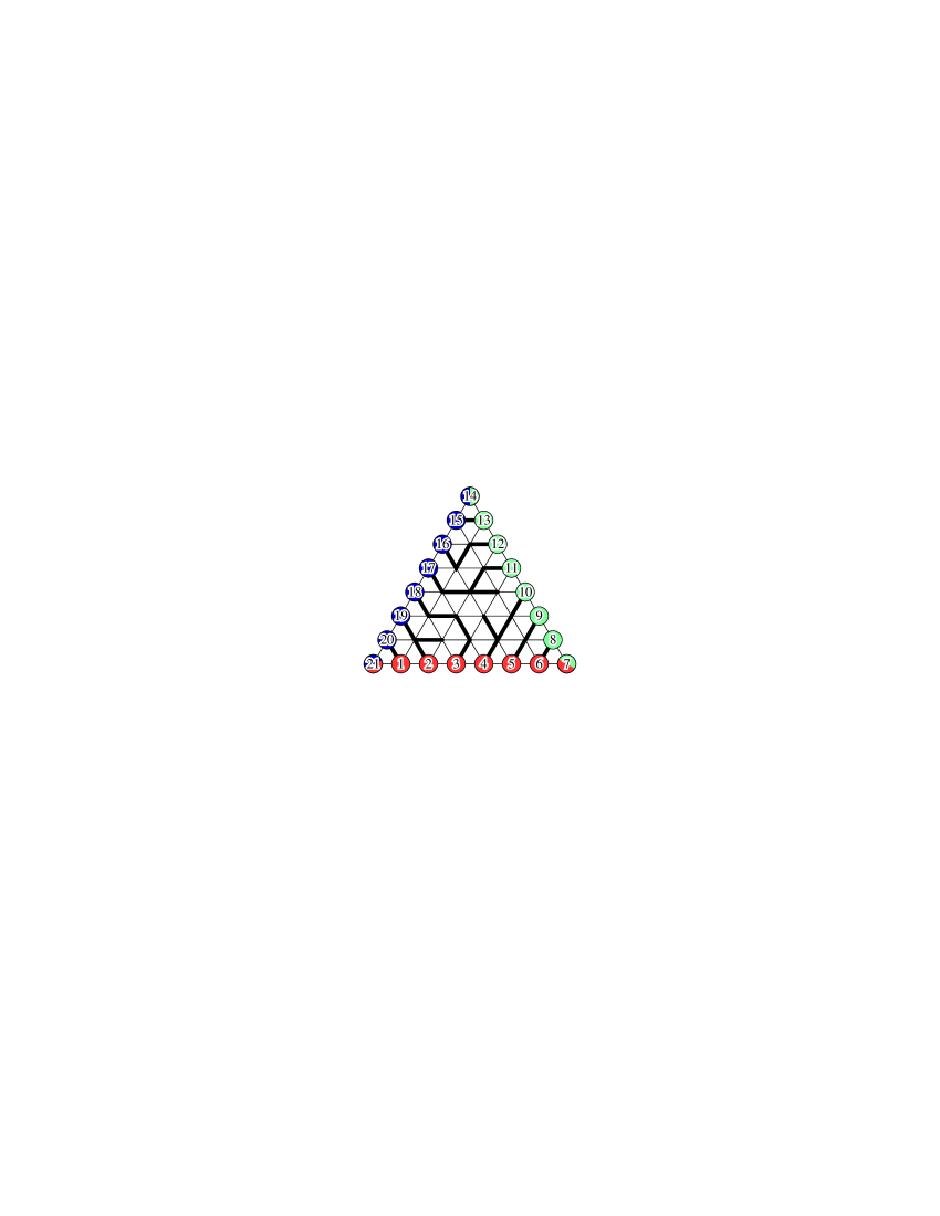
Figure 7: Carroll-Speyer graph for $N=6$ (left) and $N=7$ (right), each shown with one of its Caroll-Speyer groves. The graphs have $n=3N$ nodes; for even $N$ the grove partition type is a (generalized) tripod, while for odd $N$ the grove partition type is a (generalized) tripartite pairing. The number of Carroll-Speyer groves is $3^{\lfloor N^{2}/4\rfloor}$ [CS04].

We need the entries of the $L$ matrix in order to compute the connection probabilities using the Pfaffian and Pfaffianoid formulas presented in § 3 and § 4. To compute the tripartite connection probabilities, we need those entries of the $L$ matrix whose indices come from different sides of the triangle. From symmetry considerations, it suffices to consider the entries between the first two sides. In the $N=6$ example from Figure 7, the submatrix of the $L$ matrix with rows indexed by the nodes on side 1 (excluding corners) and columns indexed by the nodes on side 2 (excluding corners) is given by

$$\begin{bmatrix}L_{1,7}&L_{1,8}&L_{1,9}&L_{1,10}&L_{1,11}\\ L_{2,7}&L_{2,8}&L_{2,9}&L_{2,10}&L_{2,11}\\ L_{3,7}&L_{3,8}&L_{3,9}&L_{3,10}&L_{3,11}\\ L_{4,7}&L_{4,8}&L_{4,9}&L_{4,10}&L_{4,11}\\ L_{5,7}&L_{5,8}&L_{5,9}&L_{5,10}&L_{5,11}\end{bmatrix} =\begin{bmatrix}\frac{31}{9456}&\frac{25}{2364}&\frac{23}{1576}&\frac{25}{2364}&\frac{31}{9456}\\ \frac{37}{2364}&\frac{445}{9456}&\frac{23}{394}&\frac{355}{9456}&\frac{25}{2364}\\ \frac{87}{1576}&\frac{53}{394}&\frac{97}{788}&\frac{23}{394}&\frac{23}{1576}\\ \frac{529}{2364}&\frac{3043}{9456}&\frac{53}{394}&\frac{445}{9456}&\frac{25}{2364}\\ \frac{11167}{9456}&\frac{529}{2364}&\frac{87}{1576}&\frac{37}{2364}&\frac{31}{9456}\end{bmatrix}$$

$$=\begin{bmatrix}\phantom{-2015}\mathchoice{\hbox to0.0pt{\hss$\displaystyle{1}$}}{\hbox to0.0pt{\hss$\textstyle{1}$}}{\hbox to0.0pt{\hss$\scriptstyle{1}$}}{\hbox to0.0pt{\hss$\scriptscriptstyle{1}$}}&\phantom{-2015}\mathchoice{\hbox to0.0pt{\hss$\displaystyle{-1}$}}{\hbox to0.0pt{\hss$\textstyle{-1}$}}{\hbox to0.0pt{\hss$\scriptstyle{-1}$}}{\hbox to0.0pt{\hss$\scriptscriptstyle{-1}$}}&\phantom{-208}\mathchoice{\hbox to0.0pt{\hss$\displaystyle{1}$}}{\hbox to0.0pt{\hss$\textstyle{1}$}}{\hbox to0.0pt{\hss$\scriptstyle{1}$}}{\hbox to0.0pt{\hss$\scriptscriptstyle{1}$}}&\phantom{-31}\mathchoice{\hbox to0.0pt{\hss$\displaystyle{-1}$}}{\hbox to0.0pt{\hss$\textstyle{-1}$}}{\hbox to0.0pt{\hss$\scriptstyle{-1}$}}{\hbox to0.0pt{\hss$\scriptscriptstyle{-1}$}}&\phantom{-}1\\ \phantom{-2015}\mathchoice{\hbox to0.0pt{\hss$\displaystyle{-31}$}}{\hbox to0.0pt{\hss$\textstyle{-31}$}}{\hbox to0.0pt{\hss$\scriptstyle{-31}$}}{\hbox to0.0pt{\hss$\scriptscriptstyle{-31}$}}&\phantom{-2015}\mathchoice{\hbox to0.0pt{\hss$\displaystyle{24}$}}{\hbox to0.0pt{\hss$\textstyle{24}$}}{\hbox to0.0pt{\hss$\scriptstyle{24}$}}{\hbox to0.0pt{\hss$\scriptscriptstyle{24}$}}&\phantom{-208}\mathchoice{\hbox to0.0pt{\hss$\displaystyle{-16}$}}{\hbox to0.0pt{\hss$\textstyle{-16}$}}{\hbox to0.0pt{\hss$\scriptstyle{-16}$}}{\hbox to0.0pt{\hss$\scriptscriptstyle{-16}$}}&\phantom{-31}\mathchoice{\hbox to0.0pt{\hss$\displaystyle{8}$}}{\hbox to0.0pt{\hss$\textstyle{8}$}}{\hbox to0.0pt{\hss$\scriptstyle{8}$}}{\hbox to0.0pt{\hss$\scriptscriptstyle{8}$}}&-1\\ \phantom{-2015}\mathchoice{\hbox to0.0pt{\hss$\displaystyle{361}$}}{\hbox to0.0pt{\hss$\textstyle{361}$}}{\hbox to0.0pt{\hss$\scriptstyle{361}$}}{\hbox to0.0pt{\hss$\scriptscriptstyle{361}$}}&\phantom{-2015}\mathchoice{\hbox to0.0pt{\hss$\displaystyle{-208}$}}{\hbox to0.0pt{\hss$\textstyle{-208}$}}{\hbox to0.0pt{\hss$\scriptstyle{-208}$}}{\hbox to0.0pt{\hss$\scriptscriptstyle{-208}$}}&\phantom{-208}\mathchoice{\hbox to0.0pt{\hss$\displaystyle{81}$}}{\hbox to0.0pt{\hss$\textstyle{81}$}}{\hbox to0.0pt{\hss$\scriptstyle{81}$}}{\hbox to0.0pt{\hss$\scriptscriptstyle{81}$}}&\phantom{-31}\mathchoice{\hbox to0.0pt{\hss$\displaystyle{-16}$}}{\hbox to0.0pt{\hss$\textstyle{-16}$}}{\hbox to0.0pt{\hss$\scriptstyle{-16}$}}{\hbox to0.0pt{\hss$\scriptscriptstyle{-16}$}}&\phantom{-}1\\ \phantom{-2015}\mathchoice{\hbox to0.0pt{\hss$\displaystyle{-2015}$}}{\hbox to0.0pt{\hss$\textstyle{-2015}$}}{\hbox to0.0pt{\hss$\scriptstyle{-2015}$}}{\hbox to0.0pt{\hss$\scriptscriptstyle{-2015}$}}&\phantom{-2015}\mathchoice{\hbox to0.0pt{\hss$\displaystyle{888}$}}{\hbox to0.0pt{\hss$\textstyle{888}$}}{\hbox to0.0pt{\hss$\scriptstyle{888}$}}{\hbox to0.0pt{\hss$\scriptscriptstyle{888}$}}&\phantom{-208}\mathchoice{\hbox to0.0pt{\hss$\displaystyle{-208}$}}{\hbox to0.0pt{\hss$\textstyle{-208}$}}{\hbox to0.0pt{\hss$\scriptstyle{-208}$}}{\hbox to0.0pt{\hss$\scriptscriptstyle{-208}$}}&\phantom{-31}\mathchoice{\hbox to0.0pt{\hss$\displaystyle{24}$}}{\hbox to0.0pt{\hss$\textstyle{24}$}}{\hbox to0.0pt{\hss$\scriptstyle{24}$}}{\hbox to0.0pt{\hss$\scriptscriptstyle{24}$}}&-1\\ \phantom{-2015}\mathchoice{\hbox to0.0pt{\hss$\displaystyle{5297}$}}{\hbox to0.0pt{\hss$\textstyle{5297}$}}{\hbox to0.0pt{\hss$\scriptstyle{5297}$}}{\hbox to0.0pt{\hss$\scriptscriptstyle{5297}$}}&\phantom{-2015}\mathchoice{\hbox to0.0pt{\hss$\displaystyle{-2015}$}}{\hbox to0.0pt{\hss$\textstyle{-2015}$}}{\hbox to0.0pt{\hss$\scriptstyle{-2015}$}}{\hbox to0.0pt{\hss$\scriptscriptstyle{-2015}$}}&\phantom{-208}\mathchoice{\hbox to0.0pt{\hss$\displaystyle{361}$}}{\hbox to0.0pt{\hss$\textstyle{361}$}}{\hbox to0.0pt{\hss$\scriptstyle{361}$}}{\hbox to0.0pt{\hss$\scriptscriptstyle{361}$}}&\phantom{-31}\mathchoice{\hbox to0.0pt{\hss$\displaystyle{-31}$}}{\hbox to0.0pt{\hss$\textstyle{-31}$}}{\hbox to0.0pt{\hss$\scriptstyle{-31}$}}{\hbox to0.0pt{\hss$\scriptscriptstyle{-31}$}}&\phantom{-}1\end{bmatrix}^{-1}.$$

We explain here why the inverse of this submatrix is integer-valued, and how to interpret the entries.

Recall Theorem 8.1 on minors of the $L$ matrix. Letting $A$, $B$, and $C$ denote the nodes on the first, second, and third sides respectively,

$$\det[L_{i,j}]^{i\in A}_{j\in B}=\frac{Z(\text{nodes of $A$ paired with nodes of $B$, nodes of $C$ singletons})}{Z(\operatorname{uncrossing})}=\frac{1}{Z(\operatorname{uncrossing})}.$$

Likewise

$$\det[L_{i,j}]^{i\in A\setminus\{i_{0}\}}_{j\in B\setminus\{j_{0}\}}=\frac{Z\left(\genfrac{}{}{0.0pt}{0}{\text{nodes of $A\setminus\{i_{0}\}$ paired with nodes of $B\setminus\{j_{0}\}$,}}{\text{nodes of $C\cup\{i_{0},j_{0}\}$ singletons}}\right)}{Z(\operatorname{uncrossing})}.$$

Thus the $i_{0},j_{0}$ entry of the inverse of the above matrix is

$$\left([L_{i,j}]^{i\in A}_{j\in B}\right)^{-1}_{j_{0},i_{0}}=(-1)^{i_{0}+j_{0}}Z\left(\genfrac{}{}{0.0pt}{0}{\text{nodes of $A\setminus\{i_{0}\}$ paired with nodes of $B\setminus\{j_{0}\}$,}}{\text{nodes of $C\cup\{i_{0},j_{0}\}$ singletons}}\right).$$

When there are edge weights, the $i_{0},j_{0}$ entry of the inverse matrix will be given by the corresponding polynomial in the edge weights.

To get the normalized probability of the tripartite partition (for odd $N$), the Pfaffian we need is

$$\operatorname{Pf}\begin{bmatrix}\phantom{-}0&\phantom{-}L_{A,B}&\phantom{-}L_{A,C}\\ -L_{B,A}&\phantom{-}0&\phantom{-}L_{B,C}\\ -L_{C,A}&-L_{C,B}&\phantom{-}0\end{bmatrix}=\operatorname{Pf}\begin{bmatrix}\phantom{-}0&\phantom{-}L_{A,B}&\phantom{-}L_{A,B}^{T}\\ -L_{A,B}^{T}&\phantom{-}0&\phantom{-}L_{A,B}\\ -L_{A,B}&-L_{A,B}^{T}&\phantom{-}0\end{bmatrix}$$

which in the case $N=7$ gives $\ddddot{\Pr}(\text{tripartite grove})=531441/135418115000$. The calculations for the tripod partitions for even $N$ is similar, except that we take a Pfaffianoid rather than a Pfaffian.

To compute the number (as opposed to probability) of groves of a given type, we also need the number of spanning forests rooted at the nodes. The number of spanning forests may be computed from the graph Laplacian using the matrix-tree theorem, which yields the following formula

$$\prod_{\begin{subarray}{c}\{\alpha,\beta,\gamma\}\\ \alpha^{3N)}=1\\ (\alpha/\beta)^{N}=1\\ \alpha\beta\gamma=1\\ \alpha,\beta,\gamma\text{\ distinct}\end{subarray}}(6-\alpha-\alpha^{-1}-\beta-\beta^{-1}-\gamma-\gamma^{-1})$$

(see [KPW00, § 6.9] for the derivation of a similar formula). In the case $N=7$ this formula yields $135418115000$, so there are $531441=3^{12}=3^{\lfloor 7^{2}/4\rfloor}$ tripartite groves, in agreement with Carroll and Speyer’s formula. Is it possible to derive the $3^{\lfloor N^{2}/4\rfloor}$ formula using this approach?

Appendix A Pfaffianoid formula for tripod partitions

Proof of Theorem 4.2.

Any column partition $\tau$ contributing to $\sigma$ will have $(n-1)/2$ parts (as $\sigma$ does) and no singleton parts, and as such it will consist of a single tripleton part together with doubleton parts. To determine what $\tau$ contributes to $\sigma$, we may use the following abbreviated rules. For two crossing doubletons, as in (4) we use

$$13|24\to-12|34-14|23.$$

For a crossing doubleton and a tripleton, recall (Lemmas 2.1 and 2.3) that

$$13|24 \equiv 1|234+2|134+3|124+4|123-12|34-14|23$$

$$13|245 \equiv 1|2345+2|1345+3|1245+45|123-12|345-145|23$$

so we may use the rule

$$13|245 \to 45|123-12|345-23|154$$

After we apply the $13|245$ rule, let us consider another doubleton part. If the doubleton part did not cross $13$ or $245$, it will cross none of $45$, $123$, $12$, $345$, $23$, or $154$. Otherwise it is one of the following forms:

crosses	13 $|$	245	$\to$	45 $|$	123	12 $|$	345	23 $|$	154
.5, 1.5	y $|$	n		n $|$	y	y $|$	n	n $|$	y
.5, 2.5	y $|$	y		n $|$	y	n $|$	n	y $|$	y
.5, 3.5	n $|$	y		n $|$	n	n $|$	y	n $|$	y
.5, 4.5	n $|$	y		y $|$	n	n $|$	y	n $|$	y
1.5, 2.5	n $|$	y		n $|$	y	y $|$	n	y $|$	n
1.5, 3.5	y $|$	y		n $|$	y	y $|$	y	n $|$	n
1.5, 4.5	y $|$	y		y $|$	y	y $|$	y	n $|$	y
2.5, 3.5	y $|$	n		n $|$	y	n $|$	y	y $|$	n
2.5, 4.5	y $|$	y		y $|$	y	n $|$	y	y $|$	y
3.5, 4.5	n $|$	y		y $|$	n	n $|$	y	n $|$	y

In each case the doubleton part crosses at most as many other parts in the new partitions as it did in the old partition. Thus the number of crossing parts strictly decreases.

After we apply the $13|24$ rule, we saw already that the number of crossings amongst doubleton parts strictly decreases. Now let us consider crossings amongst doubleton parts and the tripleton part. The tripleton part divides the vertices into three sectors. The distribution of $1,2,3,4$ amongst these sectors is one of

• All four endpoints in same sector. Before rule neither of the chords 13,24 cross the tripleton, nor do any of them after the rule.

• Three endpoints in same sector. Before rule one chord crosses tripleton, after rule one chord crosses tripleton.

• At least one sector contains exactly two endpoints. If we apply the rule then it must be that the chords crossed, so both chords cross the tripleton. After rule, in one partition two chords cross tripleton, in other partition neither chord crosses tripleton.

In any event, the total number of crossing parts strictly decreases.

We may repeatedly apply the $13|245$ rule and $13|24$ rule, in any order, until no two parts cross, and we are guaranteed to obtain a linear combination of planar partitions containing a tripleton part and rest doubleton parts.

Recall the rule

$$13|245\to 45|123-12|345-23|154.$$

Suppose that at least one of these parts has two or more vertices of the same color, say red. We have the following possibilities:

$$\overset{r}{1}\overset{r}{3}|\overset{r}{2}45 \to 45|\overset{r}{1}\overset{r}{2}\overset{r}{3}-\overset{r}{1}\overset{r}{2}|\overset{r}{3}45-\overset{r}{2}\overset{r}{3}|\overset{r}{1}54$$

$$13|2\overset{r}{4}\overset{r}{5} \to\overset{r}{4}\overset{r}{5}|123-12|3\overset{r}{4}\overset{r}{5}-23|1\overset{r}{5}\overset{r}{4}$$

$$1\overset{r}{3}|\overset{r}{2}\overset{r}{4}5 \to\overset{r}{4}5|1\overset{r}{2}\overset{r}{3}-1\overset{r}{2}|\overset{r}{3}\overset{r}{4}5-\overset{r}{2}\overset{r}{3}|15\overset{r}{4}$$

$$\overset{r}{1}3|\overset{r}{2}4\overset{r}{5} \to 4\overset{r}{5}|\overset{r}{1}\overset{r}{2}3-\overset{r}{1}\overset{r}{2}|34\overset{r}{5}-\overset{r}{2}3|\overset{r}{1}\overset{r}{5}4$$

(the remaining cases contain more reds than these). In each case, each of the resulting partitions has a part with two or more vertices of the same color, so by induction, such partitions will not contribute to $\sigma$. Thus we may restrict attention to partitions $\tau$ with bichromatic doubleton parts and a trichromatic tripleton part.

We take another look at the rule

$$13|245\to 45|123-12|345-23|154.$$

Two colors occur twice. There are three possibilities (up to renamings of color):

	5,1 red and 3,4 blue	in which case we may use the rule $13|245\to 45|123$
($*$)	5,1 red and 2,3 blue	in which case we may use the rule $13|245\to-12|345$
($**$)	1,2 red and 3,4 blue	in which case we may use the rule $13|245\to-23|154$

(And similarly for the $13|24$ rule, either $13|24\to-12|34$ or $13|24\to-14|23$.)

Thus each maximally multichromatic partition $\tau$ contributes either $+1$ or $-1$ to $\sigma$.

Let us compare the contributions to $\sigma$ of partitions $\tau$ which contain doubleton parts that do not cross one another, and a tripleton part which may cross the doubleton parts. Any such partition $\tau$ may be obtained from $\sigma$ by repeatedly transposing items of the tripleton with their neighbors. From the above rules ($*$) and ($**$) we see that each such transposition changes the sign of $\tau$’s contribution to $\sigma$.

Next we consider what happens if we leave the tripleton part alone and only apply the $13|24$ rule. Upon deleting the tripleton part, and recalling our earlier analysis of the tripartite pairing (Theorem 3.1), we see that each partition $\tau$ contributes to $\sigma$ a sign which involves moving the tripod to its desired location in $\sigma$, times the sign in the corresponding Pfaffian in which rows and columns of items of tripleton part have been deleted. This gives us the tripod Pfaffianoid formula:

$$(-1)^{\text{sum of items in $\sigma$'s tripleton part}}\times\\ \sum_{a\in R,b\in G,c\in B}(-1)^{a+b+c}(L_{a,b}L_{b,c}+L_{a,b}L_{a,c}+L_{a,c}L_{b,c})\operatorname{Pf}(R\smallsetminus\{a\};G\smallsetminus\{b\};B\smallsetminus\{c\}).$$

∎

Appendix B Tripartite pairings in terms of Pfaffians in the resistances

There is a formula analogous to the one in Theorem 3.1 for the probability of a tripartite partition, expressing it in terms of the pairwise electrical resistances $R_{i,j}$ rather than the response matrix entries $L_{i,j}$. The normalization is also different, rather than normalizing by $\Pr(1|2|\cdots|n)$, we normalize by $\Pr(12\cdots n)$. The corresponding formula is illustrated by the following example:

$$\frac{\Pr(16|23|45)}{\Pr(123456)}=\\ [t]\operatorname{Pf}\!\left[\begin{matrix}0&0&\phantom{+}t-\frac{1}{2}R_{1,3}&\phantom{+}t-\frac{1}{2}R_{1,4}&\phantom{+}t-\frac{1}{2}R_{1,5}&\phantom{+}t-\frac{1}{2}R_{1,6}\\ 0&0&\phantom{+}t-\frac{1}{2}R_{2,3}&\phantom{+}t-\frac{1}{2}R_{2,4}&\phantom{+}t-\frac{1}{2}R_{2,5}&\phantom{+}t-\frac{1}{2}R_{2,6}\\ -t+\frac{1}{2}R_{1,3}&-t+\frac{1}{2}R_{2,3}&0&0&\phantom{+}t-\frac{1}{2}R_{3,5}&\phantom{+}t-\frac{1}{2}R_{3,6}\\ -t+\frac{1}{2}R_{1,4}&-t+\frac{1}{2}R_{2,4}&0&0&\phantom{+}t-\frac{1}{2}R_{4,5}&\phantom{+}t-\frac{1}{2}R_{4,6}\\ -t+\frac{1}{2}R_{1,5}&-t+\frac{1}{2}R_{2,5}&-t+\frac{1}{2}R_{3,5}&-t+\frac{1}{2}R_{4,5}&0&0\\ -t+\frac{1}{2}R_{1,6}&-t+\frac{1}{2}R_{2,6}&-t+\frac{1}{2}R_{3,6}&-t+\frac{1}{2}R_{4,6}&0&0\end{matrix}\right]$$ (10)

Here the Pfaffian is a polynomial in $t$, in fact a linear function of $t$, and the coefficient of the linear term gives $\Pr(16|23|45)/\Pr(123456)$.

We prove here this formula when one of the color classes is empty, so that the Pfaffian is actually a determinant (see Theorem B.3). The general tripartite Pfaffian formula follows from the bipartite determinant special case, together with a result that we prove in our next article that for any planar pairing, the $L$-polynomial is a linear combination of such determinants [KW08].

Recall that any codimension-1 minor of $L$ is the ratio of the spanning trees to the uncrossing. Let $\tilde{L}$ be the $(n-1)\times(n-1)$ submatrix of $L$ obtained by deleting the last row and column. Recall that $R_{i,j}={\tilde{L}}^{-1}_{i,i}+{\tilde{L}}^{-1}_{j,j}-2{\tilde{L}}^{-1}_{i,j}$, where ${\tilde{L}}^{-1}_{i,j}$ is interpreted to be $0$ if either $i=n$ or $j=n$ (see [KW06, Section A.2]).

Lemma B.1.

For each row of $I+LR/2$, the row’s entries are all the same.

Proof.

Suppose $i\neq n$. Then

$$\sum_{j}L_{i,j}R_{j,k} =\sum_{j}L_{i,j}[{\tilde{L}}^{-1}_{j,j}+{\tilde{L}}^{-1}_{k,k}-2{\tilde{L}}^{-1}_{j,k}]$$

$$=\sum_{j}L_{i,j}[R_{j,n}+0]-2\delta_{i,k}.$$

So for any $i\neq n$, the $i$${}^{\text{th}}$ row of $I+LR/2$ is constant. By re-indexing the rows, we see that this must hold for the $n$${}^{\text{th}}$ row as well. ∎

Lemma B.2.

The diagonal entries of $RLR$ are all the same.

Proof.

We have

$$\sum_{j,k}R_{i,j}L_{j,k}R_{k,i} =\sum_{j,k}({\tilde{L}}^{-1}_{i,i}+{\tilde{L}}^{-1}_{j,j}-2{\tilde{L}}^{-1}_{i,j})L_{j,k}({\tilde{L}}^{-1}_{i,i}+{\tilde{L}}^{-1}_{k,k}-2{\tilde{L}}^{-1}_{i,k}).$$

The third factor contains no $j$ subscripts, and neither does the ${\tilde{L}}^{-1}_{i,i}$ term of the first factor, so summing over $j$ gives $0$, and we may drop the ${\tilde{L}}^{-1}_{i,i}$ term in the first factor. Similarly, we may drop the ${\tilde{L}}^{-1}_{i,i}$ term in the third factor.

$$\sum_{j,k}R_{i,j}L_{j,k}R_{k,i} =\sum_{j,k}({\tilde{L}}^{-1}_{j,j}-2{\tilde{L}}^{-1}_{i,j})L_{j,k}({\tilde{L}}^{-1}_{k,k}-2{\tilde{L}}^{-1}_{i,k})$$

$$=\sum_{j,k}{\tilde{L}}^{-1}_{j,j}L_{j,k}{\tilde{L}}^{-1}_{k,k}-2\sum_{j,k}{\tilde{L}}^{-1}_{j,j}L_{j,k}{\tilde{L}}^{-1}_{i,k}-2\sum_{j,k}{\tilde{L}}^{-1}_{i,j}L_{j,k}({\tilde{L}}^{-1}_{k,k}-2{\tilde{L}}^{-1}_{i,k})$$

$$=\sum_{j,k}{\tilde{L}}^{-1}_{j,j}L_{j,k}{\tilde{L}}^{-1}_{k,k}-2\sum_{j}{\tilde{L}}^{-1}_{j,j}\delta_{j,i}-2\sum_{k}\delta_{i,k}({\tilde{L}}^{-1}_{k,k}-2{\tilde{L}}^{-1}_{i,k})$$

$$=\sum_{j,k}{\tilde{L}}^{-1}_{j,j}L_{j,k}{\tilde{L}}^{-1}_{k,k}$$

which in particular does not depend upon $i$: the diagonal terms of $RLR$ are all equal. ∎

Suppose that we add an extra $(n+1)$${}^{\text{st}}$ node to the graph where the conductance between nodes $j$ and $n+1$ is $\varepsilon(1+\frac{1}{2}\sum_{k}L_{j,k}R_{j,k})$, where $\varepsilon\approx 0$. (Some of these conductances may be negative.) From Lemma B.1 we have

$$\delta_{i,j}+\frac{1}{2}\sum_{k}L_{j,k}R_{k,i} =1+\frac{1}{2}\sum_{k}L_{j,k}R_{j,k}$$

$$1=\sum_{j}\left[\delta_{i,j}+\frac{1}{2}\sum_{k}L_{j,k}R_{k,i}\right] =\sum_{j}\left[1+\frac{1}{2}\sum_{k}L_{j,k}R_{j,k}\right],$$

so adding up the conductances of these new edges gives $\varepsilon$. If we set node $n+1$ to be at $1$ volt and node $i$ to be at $0$ volts, then to first order, each of the nodes $1,\dots,n$ be nearly at $0$ volts. Then the current flowing from node $n+1$ to node $j$ is $(1+o(1))\varepsilon(\delta_{i,j}+\frac{1}{2}\sum_{k}L_{j,k}R_{k,i})$, and the total current from node $n+1$ is $(1+o(1))\varepsilon$. Let $v$ denote the voltages of the first $n$ nodes. Now we view the first $n$ nodes as a circuit to which we apply the voltages $v$. The current flowing into node $j\neq i$ is $(1+o(1))\frac{\varepsilon}{2}\sum_{k}L_{j,k}R_{k,i}$, and the current flowing into node $i$ is $(1+o(1))\varepsilon(1+\frac{1}{2}\sum_{k}L_{i,k}R_{k,i})-(1+o(1))\varepsilon$ (the first term is the current from the $(n+1)$${}^{\text{st}}$ node to node $i$, and the second term is the current flowing out of node $i$, i.e., the total current flowing in from node $(n+1)$). To summarize, we have

$$Lv=(1+o(1))\frac{1}{2}\varepsilon LR\delta_{i},$$

where $\delta_{i}$ is the $i$${}^{\text{th}}$ basis vector. We would like to cancel the $L$’s from this equation, but the equation only determines $v$ up to an additive constant: $v=\frac{1}{2}\varepsilon R\delta_{i}+o(\varepsilon)+\text{const}$. But $v_{i}=0$ and $R_{i,i}=0$, so the additive constant is zero. Knowing the voltages $v_{j}=\frac{1}{2}\varepsilon R_{i,j}+o(\varepsilon)$ allows us to compute the currents to second order: the total current from node $n+1$ is

$$\sum_{j}\varepsilon\left[\delta_{i,j}+\frac{1}{2}\sum_{k}L_{j,k}R_{k,i}\right]\left(1-\frac{\varepsilon}{2}R_{i,j}+o(\varepsilon)\right) =\varepsilon-\frac{\varepsilon^{2}}{4}\sum_{j,k}R_{i,j}L_{j,k}R_{k,i}+o(\varepsilon^{2})$$

$$=\varepsilon-\frac{\varepsilon^{2}}{4}Q+o(\varepsilon^{2})$$

where $Q$ is the diagonal entry of $RLR$. Let $\tilde{R}$ denote the resistances in the extended graph; we have

$$\tilde{R}_{i,n+1}=1/\varepsilon+Q/4+o(1).$$

Let $\tilde{L}$ be the $L$-matrix of the enlarged graph, $\tilde{L}^{\prime}$ be the submatrix obtained by deleting the $(n+1)$${}^{\text{st}}$ vertex, and $\tilde{L}^{\prime-1}$ be the inverse of $\tilde{L}^{\prime}$ (sometimes extended to have an all-$0$ $(n+1)$${}^{\text{st}}$ row and column). The ratio of spanning trees to the uncrossing is

$$\lim_{\varepsilon\to 0}\frac{1}{\varepsilon}\det(-\tilde{L}^{\prime}) =\lim_{\varepsilon\to 0}\frac{1}{\varepsilon}\frac{1}{\det(-\tilde{L}^{\prime-1})}$$

now recall $$(-\tilde{L}^{\prime-1})_{i,j}=(\tilde{R}_{i,n+1}+\tilde{R}_{j,n+1}-\tilde{R}_{i,j})/2$$, so

$$=\lim_{\varepsilon\to 0}\frac{1}{\varepsilon}\frac{1}{\det[1/\varepsilon+Q/4-R_{i,j}/2+o(1)]^{i=1,\dots,n}_{j=1,\dots,n}}.$$

This determinant is a linear function of $$t=1/\varepsilon+Q/4$$, so we may rewrite this limit as

$$=\frac{1}{[t]\det[t-{\textstyle\frac{1}{2}}R_{i,j}]^{i=1,\dots,n}_{j=1,\dots,n}}.$$

Let $A$ and $B$ be two subsets of the nodes. We have

$$\det[L_{i,j}]^{i\in A}_{j\in B}= \lim_{\varepsilon\to 0}\det[\tilde{L}^{\prime}_{i,j}]^{i\in A}_{j\in B}$$

$$= \lim_{\varepsilon\to 0}\det\tilde{L}^{\prime}\det[\tilde{L}^{\prime-1}_{j,i}]^{j\in B^{c}}_{i\in A^{c}}\times(-1)^{\sum_{a\in A}a+\sum_{b\in B}b}$$

$$= \lim_{\varepsilon\to 0}\frac{\varepsilon}{[t]\det[t-{\textstyle\frac{1}{2}}R_{i,j}]^{i=1,\dots,n}_{j=1,\dots,n}}\det[-1/\varepsilon-Q/4+R_{i,j}/2+o(1)]^{j\in B^{c}}_{i\in A^{c}}$$

$$\ \ \ \ \ \times(-1)^{\sum_{a\in A}a+\sum_{b\in B}b}$$

$$= \frac{[t]\det[-t+{\textstyle\frac{1}{2}}R_{i,j}]^{j\in B^{c}}_{i\in A^{c}}}{[t]\det[t-{\textstyle\frac{1}{2}}R_{i,j}]^{i=1,\dots,n}_{j=1,\dots,n}}\times(-1)^{\sum_{a\in A}a+\sum_{b\in B}b},$$ (11)

where in the above, the rows and columns in $A$, $B$, $A^{c}$, and $B^{c}$ are arranged in sorted order.

Note that (11) allows us to rewrite any minor of the $L$ matrix in terms of the pairwise resistances between the nodes. Since the denominator of the right-hand side of (11) is $Z(\operatorname{uncrossing})/Z(\operatorname{tree})$, we have

$$\frac{Z(\operatorname{uncrossing})}{Z(\operatorname{tree})}\det[L_{i,j}]^{i\in A}_{j\in B}=[t]\det[-t+{\textstyle\frac{1}{2}}R_{i,j}]^{j\in B^{c}}_{i\in A^{c}}\times(-1)^{\sum_{a\in A}a+\sum_{b\in B}b}.$$ (12)

If $A=B^{c}$, then (12) simplifies to yield

Theorem B.3.

If $A$ and $B$ are disjoint and equinumerous sets of nodes and $A\cup B$ is the set of all nodes, then

$$\frac{Z(\operatorname{uncrossing})}{Z(\operatorname{tree})}\det[L_{i,j}]^{i\in A}_{j\in B}=[t]\det[t-{\textstyle\frac{1}{2}}R_{i,j}]^{i\in A}_{j\in B}.$$

References

- [CdV98] Yves Colin de Verdière. Spectres de graphes, volume 4 of Cours Spécialisés [Specialized Courses]. Société Mathématique de France, Paris, 1998. MR1652692 (99k:05108)
- [CdVGV96] Yves Colin de Verdière, Isidoro Gitler, and Dirk Vertigan. Réseaux électriques planaires. II. Comment. Math. Helv., 71(1):144–167, 1996. MR1371682 (98a:05054)
- [Cha82] Seth Chaiken. A combinatorial proof of the all minors matrix tree theorem. SIAM J. Algebraic Discrete Methods, 3(3):319–329, 1982. MR666857 (83h:05062)
- [Che76] Wai Kai Chen. Applied Graph Theory: Graphs and electrical networks. North-Holland Publishing Co., Amsterdam, 2nd edition, 1976. MR0472234 (57 #11940)
- [CIM98] E. B. Curtis, D. Ingerman, and J. A. Morrow. Circular planar graphs and resistor networks. Linear Algebra Appl., 283(1-3):115–150, 1998. MR1657214 (99k:05096)
- [Ciu97] Mihai Ciucu. Enumeration of perfect matchings in graphs with reflective symmetry. J. Combin. Theory Ser. A, 77(1):67–97, 1997. MR1426739 (98a:05112)
- [CM02] Ryan K. Card and Brandon I. Muranaka. Using network amalgamation and separation to solve the inverse problem, 2002. http://www.math.washington.edu/~morrow/papers/ryanc.pdf.
- [CS04] Gabriel D. Carroll and David Speyer. The cube recurrence. Electron. J. Combin., 11(1):Research Paper 73, 31 pp., 2004, arXiv:math.CO/0403417. MR2097339 (2005f:05007)
- [DFGG97] P. Di Francesco, O. Golinelli, and E. Guitter. Meanders and the Temperley-Lieb algebra. Comm. Math. Phys., 186(1):1–59, 1997, arXiv:hep-th/9602025. MR1462755 (99f:82028)
- [Fom01] Sergey Fomin. Loop-erased walks and total positivity. Trans. Amer. Math. Soc., 353(9):3563–3583 (electronic), 2001, arXiv:math.CO/0004083. MR1837248 (2002f:15030)
- [Kas67] P. W. Kasteleyn. Graph theory and crystal physics. In Graph Theory and Theoretical Physics, pages 43–110. Academic Press, London, 1967. MR0253689 (40 #6903)
- [KPW00] Richard W. Kenyon, James G. Propp, and David B. Wilson. Trees and matchings. Electron. J. Combin., 7:Research Paper 25, 34 pp., 2000, arXiv:math.CO/9903025. MR1756162 (2001a:05123)
- [Kuo04] Eric H. Kuo. Applications of graphical condensation for enumerating matchings and tilings. Theoretical Computer Science, 319(1-3):29–57, 2004, arXiv:math.CO/0304090.
- [Kuo06] Eric H. Kuo. Graphical condensation generalizations involving Pfaffians and determinants, 2006. http://math.gmu.edu/~ekuo/pfaff.pdf.
- [KW06] Richard W. Kenyon and David B. Wilson. Boundary partitions in trees and dimers, 2006, arXiv:math.PR/0608422. Trans. Amer. Math. Soc., to appear.
- [KW08] Richard W. Kenyon and David B. Wilson. Marginal pairing probabilities for trees and dimers, 2008. Manuscript.
- [PS05] T. Kyle Petersen and David Speyer. An arctic circle theorem for Groves. J. Combin. Theory Ser. A, 111(1):137–164, 2005, arXiv:math.CO/0407171. MR2144860 (2006m:05055)
- [Rus03] Jeffrey T. Russell. and solve the inverse problem, 2003. http://www.math.washington.edu/~reu/papers/2003/russell/recovery.pdf.