A symplectic integration method for elastic filaments

Abstract

A new method is proposed for integrating the equations of motion of an elastic filament. In the standard finite-difference and finite-element formulations the continuum equations of motion are discretized in space and time, but it is then difficult to ensure that the Hamiltonian structure of the exact equations is preserved. Here we discretize the Hamiltonian itself, expressed as a line integral over the contour of the filament. This discrete representation of the continuum filament can then be integrated by one of the explicit symplectic integrators frequently used in molecular dynamics. The model systematically approximates the continuum partial differential equations, but has the same level of computational complexity as molecular dynamics and is constraint free. Numerical tests show that the algorithm is much more stable than a finite-difference formulation and can be used for high aspect ratio filaments, such as actin.

I Introduction

Elastic rods are a ubiquitous model of semi-flexible biopolymers such as DNA,Marko1994a ; Marko1995 ; Swigon1998 ; Balaeff1999 ; Coleman2000 ; Tobias2000a ; Coleman2003 ; Rossetto2003 actin,Isambert1995 ; Maggs1998 ; Gardel2004 ; DiDonna2007 and microtubules.Brangwynne2006 They can also be found in a diverse range of applications including catheter navigation,Lawton1999 undersea cables,Goyal2008 and organismal biology.Goriely2006 In biophysics, the worm-like chain (WLC) modelMarko1994 ; Marko1995 underpins many theoreticalLevine2004a ; Head2005 ; Storm2005 ; DiDonna2006 ; DiDonna2007 ; Das2007 ; Mizuno2007 ; MacKintosh2008 and numericalEveraers1999 ; Wada2006 ; Wada2007a ; Llopis2007 studies of semiflexible polymers. The WLC model is a linearization of the classical Kirchoff rod model,Love1944 ; Landau1959 which is itself a limiting case where the product of the local curvature and filament thickness is everywhere small.Coleman1993 In this limit the shear and extensional strains are negligible but the constraint forces generated by them are not. In this paper we consider a generalization of the Kirchoff model,Romero2002 ; Bishop2004 where the shear and extensional strains are explicitly accounted for by an elastic constitutive model, eliminating the need for constraint forces at the cost of an additional time scale; such models are frequently referred to as “geometrically exact” in the finite-element literature.Romero2002 ; Bishop2004

The dynamics of Kirchoff or geometrically exact (GE) filaments is typically determined by finite-element or finite-difference approximations, but the stiffness of the numerical system has proved to be a difficult and long-standing problem.Simo1988 ; Simo1995 Significant progress has been made by developing implicit methods that exactly satisfy the constraints of momentum and energy conservation,Romero2002 ; Goyal2005 yet even here artificial dissipation is often needed for long-term stability.Armero2003 On the other hand, in discrete dynamical systems it is known that symplectic integration methods give superior long-term stability in comparison with either high-order explicit or implicit integration methods;Dullweber1997 the most common symplectic integrator is the Verlet algorithm.Verlet1967 Symplectic integrators generate a sequence of canonical transformations, which do not exactly conserve energy but do preserve the density of points in the phase space, along with the Poincaré invariants. In recent years symplectic integrators have been developed for both linear and angular motions.Dullweber1997 ; Miller2002 ; Zon2008 The objective of this paper is to explore a symplectic integration method for geometrically exact filament models. This requires both a Hamiltonian approximation to the partial differential equations describing the filament dynamics, and a symplectic integrator.

The proposed algorithm is based on a discretization of the Hamiltonian line integral of an elastic filament, including shear and extensional degrees of freedom. Since the nodal forces and torques follow from an exact differentiation of a potential function, the equations of motion are guaranteed to be Hamiltonian, although the potential function itself is only an approximation to the continuum limit. This is in contrast to finite-element methods, where the continuum equations of motion are discretized in space; in this case the Hamiltonian structure is not preserved, even if the total energy is conserved.Romero2002 In fact, it can be shown that for any approximate solution it is not possible to maintain both the symplectic structure and exact energy conservation simultaneously.Zhong1988

An outline of the paper is as follows. In Sec. II we describe different models of elastic filaments–GE, Kirchoff, WLC–and indicate how they are related. Next (Sec. III), we derive a simple finite-difference approximation of the equations of motion of a GE filament model, as a basis for comparison with the Hamiltonian formulation presented in Sec. IV. We note that the Hamiltonian approach has only been followed occasionally,Dichmann1996 and in that case for the Kirchoff rod model. We will argue (Sec. V) that the absence of geometric constraints in the GE model offers computational advantages over the Kirchoff model when there are excluded volume interactions between the segments. We replace the usual implicit time integrationDichmann1996 ; Romero2002 with an explicit operator splitting method,Miller2002 which eliminates the repeated force evaluations of an implicit method. The numerical scheme is stable and energy conserving even for large deformations; we illustrate this by numerical example in Sec. V. Our conclusions and future outlook are in Sec. VI.

II Elastic filament models

Figure 1: An elastic filament in the unstrained (reference) state (a) and after deformation (b). In the reference state, the material plane, shown by the solid ellipse, is aligned with its normal parallel to the tangent to the centerline (dashed line). The local director basis of the reference state, ${\mbox{\boldmath${d}$}}_{i}^{0}(s)$, and the deformed state, ${\mbox{\boldmath${d}$}}_{i}(s)$, are also shown. A material point (solid black circle) moves with the translation and rotation of the local coordinate system; in this case extension, shear, bend, and twist can all be seen.

The classical Kirchoff theory of elastic rods has been elegantly and concisely described in the “Theory of Elasticity” by Landau and Lifshitz,Landau1959 and the seminal book by Love.Love1944 More rigorous derivations of the equations of motion are available in the literature.Green1966 ; Coleman1993 Here we summarize the key concepts and establish the notation to be used later in the paper. An elastic filament (or thin rod) is described by the coordinates of its centerline ${\mbox{\boldmath${r}$}}(s)$ and a set of orthonormal directors ${\mbox{\boldmath${d}$}}_{1}(s)$, ${\mbox{\boldmath${d}$}}_{2}(s)$, ${\mbox{\boldmath${d}$}}_{3}(s)$. The directors establish the orientation of a cross section or material plane at the location $s$, where $s$ is a parametric coordinate defining the position of each point along the centerline. In the undeformed filament, $s$ is the contour length from the origin. We will choose a body-fixed coordinate system such that ${\mbox{\boldmath${d}$}}_{1}$ and ${\mbox{\boldmath${d}$}}_{2}$ point along the principal axes of inertia of the cross section and therefore ${\mbox{\boldmath${d}$}}_{3}={\mbox{\boldmath${d}$}}_{1}\times{\mbox{\boldmath${d}$}}_{2}$ is normal to the material plane; the coordinate system is illustrated in Fig 1. If the rod has a circular cross section then the initial choice of ${\mbox{\boldmath${d}$}}_{1}$ and ${\mbox{\boldmath${d}$}}_{2}$ contains an arbitrary rotation about ${\mbox{\boldmath${d}$}}_{3}$. In contrast with the Kirchoff theory, we will not assume that ${\mbox{\boldmath${d}$}}_{3}$ is constrained to be parallel to the tangent vector $\partial_{s}{\mbox{\boldmath${r}$}}$ (Fig 1b).

The key assumption of thin-rod elasticity is that there is no deformation within a material plane, only translation and rotation of that plane. Deformation of an elastic filament is then described by two one-dimensional strain fields, ${\mbox{\boldmath${\Gamma}$}}(s)$ and ${\mbox{\boldmath${\Omega}$}}(s)$, describing the rate of change of the centerline position and director vectors along the filamentRomero2002 ; Bishop2004

$$\begin{array}[]{ccc}\Gamma_{1}={\mbox{\boldmath${d}$}}_{1}\cdot(\partial_{s}{\mbox{\boldmath${r}$}})&{}{}{}\hfil&\Omega_{1}={\mbox{\boldmath${d}$}}_{3}\cdot(\partial_{s}{\mbox{\boldmath${d}$}}_{2})=-{\mbox{\boldmath${d}$}}_{2}\cdot(\partial_{s}{\mbox{\boldmath${d}$}}_{3})\\ \Gamma_{2}={\mbox{\boldmath${d}$}}_{2}\cdot(\partial_{s}{\mbox{\boldmath${r}$}})&{}{}{}\hfil&\Omega_{2}={\mbox{\boldmath${d}$}}_{1}\cdot(\partial_{s}{\mbox{\boldmath${d}$}}_{3})=-{\mbox{\boldmath${d}$}}_{3}\cdot(\partial_{s}{\mbox{\boldmath${d}$}}_{1})\\ \Gamma_{3}={\mbox{\boldmath${d}$}}_{3}\cdot(\partial_{s}{\mbox{\boldmath${r}$}})&{}{}{}\hfil&\Omega_{3}={\mbox{\boldmath${d}$}}_{2}\cdot(\partial_{s}{\mbox{\boldmath${d}$}}_{1})=-{\mbox{\boldmath${d}$}}_{1}\cdot(\partial_{s}{\mbox{\boldmath${d}$}}_{2}).\end{array}$$ (1)

A thin segment of the filament can be subjected to six different deformations. $\Gamma_{1}$ and $\Gamma_{2}$ describe transverse motions of a material plane with respect to the normal vector (${\mbox{\boldmath${d}$}}_{3}$), which causes shearing of the segment, while $\Gamma_{3}$ describes extension or compression of the segment. Bending of the segment about its principal axes is described by $\Omega_{1}$ and $\Omega_{2}$, and twisting of the segment by $\Omega_{3}$. Uniform deformation corresponds to constant values of ${\Gamma}$ and ${\Omega}$; for example, in a straight rod ${\mbox{\boldmath${\Gamma}$}}=[0,0,1]$ and ${\mbox{\boldmath${\Omega}$}}=[0,0,0]$. More interestingly, a helical rod can be described by a constant bend and twist, ${\mbox{\boldmath${\Gamma}$}}=[0,0,1]$, ${\mbox{\boldmath${\Omega}$}}=[R\kappa^{2},0,P\kappa^{2}]$, where $R$ is the radius of the helix, $2\pi P$ is the pitch, and the combined curvature due to bend and twist, $\kappa=(P^{2}+R^{2})^{-1/2}$. The choice of signs define a right-handed helix, ${\mbox{\boldmath${r}$}}(s)=[R\cos(\kappa s),R\sin(\kappa s),P\kappa s]$, with basis vectors

$$\begin{array}[]{l}{\mbox{\boldmath${d}$}}_{1}=[P\kappa\sin(\kappa s),-P\kappa\cos(\kappa s),R\kappa]\\ {\mbox{\boldmath${d}$}}_{2}=[\cos(\kappa s),\sin(\kappa s),0]\\ {\mbox{\boldmath${d}$}}_{3}=[-R\kappa\sin(\kappa s),R\kappa\cos(\kappa s),P\kappa].\end{array}$$ (2)

The stresses in the rod are assumed to be linear in the deviations in the strain fields, $\Delta\Gamma_{i}=\Gamma_{i}-\Gamma_{i}^{0}$ and $\Delta\Omega_{i}=\Omega_{i}-\Omega_{i}^{0}$, from the reference (stress free) configuration ${\mbox{\boldmath${\Gamma}$}}^{0}$, ${\mbox{\boldmath${\Omega}$}}^{0}$. It is convenient to define the strains in the body-fixed coordinate system, since the elastic constant matrix is then diagonal. The force $F_{i}^{\Gamma}$ and couple $F_{i}^{\Omega}$ on each material plane areLandau1959 ; Love1944

$$F_{i}^{\Gamma}=C_{i}^{\Gamma}\Delta\Gamma_{i},~{}~{}~{}F_{i}^{\Omega}=C_{i}^{\Omega}\Delta\Omega_{i},$$ (3)

where the elastic constants for each deformation are, in principle, independent. In the GE model, the strain energy density $U(s)$ contains contributions from shear and extension, in addition to the usual bend and twist of the Kirchoff model,

$$U=U^{\Gamma}+U^{\Omega}=\frac{1}{2}\sum_{i=1}^{3}\left(C_{i}^{\Gamma}\Delta\Gamma_{i}^{2}+C_{i}^{\Omega}\Delta\Omega_{i}^{2}\right).$$ (4)

For an isotropic material, the elastic moduli for shear ($C_{1,2}^{\Gamma}$), extension ($C_{3}^{\Gamma}$), bend ($C_{1,2}^{\Omega}$), and twist ($C_{3}^{\Omega}$) are given by:

$$\begin{array}[]{ccc}C_{1}^{\Gamma}=GA&{}{}{}\hfil&C_{1}^{\Omega}=YI_{1}\\ C_{2}^{\Gamma}=GA&{}{}{}\hfil&C_{2}^{\Omega}=YI_{2}\\ C_{3}^{\Gamma}=YA&{}{}{}\hfil&C_{3}^{\Omega}=GI_{3},\end{array}$$ (5)

where $G$ is the shear modulus, $Y$ is Young’s modulus, $A$ is the area of the cross-section and $I_{1}$ and $I_{2}$ are its principle moments of inertia. For rods with a circular cross section, $I_{3}=I_{1}+I_{2}$, but in the general case there is an additional contribution from the warping of the cross section,Landau1959 so that $I_{3}$ is then distinct from $I_{1}+I_{2}$. The elastic coefficients can also be determined empirically, without reference to any particular constitutive law.

The velocity and angular velocity of the segment are defined in an analogous fashion to the strain fields in Eq. 1,

$$\begin{array}[]{ccc}v_{1}={\mbox{\boldmath${d}$}}_{1}\cdot(\partial_{t}{\mbox{\boldmath${r}$}})&{}{}{}\hfil&\omega_{1}={\mbox{\boldmath${d}$}}_{3}\cdot(\partial_{t}{\mbox{\boldmath${d}$}}_{2})=-{\mbox{\boldmath${d}$}}_{2}\cdot(\partial_{t}{\mbox{\boldmath${d}$}}_{3})\\ v_{2}={\mbox{\boldmath${d}$}}_{2}\cdot(\partial_{t}{\mbox{\boldmath${r}$}})&{}{}{}\hfil&\omega_{2}={\mbox{\boldmath${d}$}}_{1}\cdot(\partial_{t}{\mbox{\boldmath${d}$}}_{3})=-{\mbox{\boldmath${d}$}}_{3}\cdot(\partial_{t}{\mbox{\boldmath${d}$}}_{1})\\ v_{3}={\mbox{\boldmath${d}$}}_{3}\cdot(\partial_{t}{\mbox{\boldmath${r}$}})&{}{}{}\hfil&\omega_{3}={\mbox{\boldmath${d}$}}_{2}\cdot(\partial_{t}{\mbox{\boldmath${d}$}}_{1})=-{\mbox{\boldmath${d}$}}_{1}\cdot(\partial_{t}{\mbox{\boldmath${d}$}}_{2}).\end{array}$$ (6)

The kinetic energy density of the filament is thenLandau1959 ; Love1944

$$T=T^{\Gamma}+T^{\Omega}=\frac{1}{2}\sum_{i=1}^{3}\left(M_{i}^{\Gamma}v_{i}^{2}+M_{i}^{\Omega}\omega_{i}^{2}\right),$$ (7)

where the generalized mass densities associated with shear ($M_{1}^{\Gamma},M_{2}^{\Gamma}$), extension ($M_{3}^{\Gamma}$), bend ($M_{1}^{\Omega},M_{2}^{\Omega}$) and twist ($M_{3}^{\Omega}$), are

$$\begin{array}[]{ccc}M_{i}^{\Gamma}=\rho A,&{}{}{}\hfil&M_{i}^{\Omega}=\rho I_{i},\end{array}$$ (8)

and $\rho$ is the mass density of the filament.

Equations of motion for the filament can be derived from the balance of linear and angular momenta in a thin segment bounded by the planes $s$ and $s+ds$. The rate of change of the linear momentum of the segment, ${\mbox{\boldmath${p}$}}ds$, is

$${\dot{\mbox{\boldmath${p}$}}}ds={\mbox{\boldmath${F}$}}^{\Gamma}(s+ds)-{\mbox{\boldmath${F}$}}^{\Gamma}(s),$$ (9)

where ${\mbox{\boldmath${p}$}}=\sum_{i=1}^{3}M^{\Gamma}v_{i}{\mbox{\boldmath${d}$}}_{i}$ is the linear momentum density (per unit length). The forces on the two planes must be differenced in a common coordinate frame, which we take as the space-fixed frame. The balance of angular momentum in the segment ${\mbox{\boldmath${l}$}}ds$ involves both couples and moments of the force,

$${\dot{\mbox{\boldmath${l}$}}}ds={\mbox{\boldmath${F}$}}^{\Omega}(s+ds)-{\mbox{\boldmath${F}$}}^{\Omega}(s)+{\mbox{\boldmath${r}$}}(s+ds)\times{\mbox{\boldmath${F}$}}^{\Gamma}(s+ds)-{\mbox{\boldmath${r}$}}(s)\times{\mbox{\boldmath${F}$}}^{\Gamma}(s),$$ (10)

where ${\mbox{\boldmath${l}$}}=\sum_{i=1}^{3}M_{i}^{\Omega}\omega_{i}{\mbox{\boldmath${d}$}}_{i}$ is the linear angular momentum density. Thus the equations of motion of a GE filament are

$${\dot{\mbox{\boldmath${p}$}}} = \partial_{s}{\mbox{\boldmath${F}$}}^{\Gamma},$$ (11)

$${\dot{\mbox{\boldmath${l}$}}} = \partial_{s}{\mbox{\boldmath${F}$}}^{\Omega}+{\mbox{\boldmath${r}$}}^{\prime}\times{\mbox{\boldmath${F}$}}^{\Gamma},$$ (12)

where ${\mbox{\boldmath${r}$}}^{\prime}=\partial_{s}{\mbox{\boldmath${r}$}}$ indicates a spatial derivative along the filament. A finite-difference approximation to these equations is described in Sec. III.

Equations 11–12 describe the dynamics of the GE rod model.Romero2002 ; Bishop2004 The difference with the Kirchoff theory is that, here, the force on a material plane, $F_{i}^{\Gamma}$, is given by a constitutive equation, Eq. (3), based on the deflection and extension of the local tangent vector relative to the material plane, Eq (1). In the Kirchoff model the tangent vector is constrained to remain parallel to ${\mbox{\boldmath${d}$}}_{3}$ (unshearable) and of unit length (inextensible), or in other words $\Delta\Gamma_{i}=0$ and ${\mbox{\boldmath${r}$}}^{\prime}={\mbox{\boldmath${d}$}}_{3}$. As a result, neighboring segments can only rotate with respect to one another, leading to a compatibility condition,Goyal2005

$${\mbox{\boldmath${v}$}}^{\prime}={\mbox{\boldmath${\omega}$}}\times{\mbox{\boldmath${r}$}}^{\prime}={\dot{\mbox{\boldmath${d}$}}}_{3},$$ (13)

where the last equality follows from the kinematic conditions, ${\dot{\mbox{\boldmath${d}$}}}_{i}={\mbox{\boldmath${\omega}$}}\times{\mbox{\boldmath${d}$}}_{i}$.Landau1959 ; Green1966 Differentiating Eq. (11) with respect to $s$ gives an equation for the constraint force satisfying the compatibility equation,

$$\partial_{s}^{2}{\mbox{\boldmath${F}$}}^{\Gamma}=M^{\Gamma}{\ddot{\mbox{\boldmath${d}$}}}_{3},$$ (14)

where ${\ddot{\mbox{\boldmath${d}$}}}_{3}={\dot{\mbox{\boldmath${\omega}$}}}\times{\mbox{\boldmath${d}$}}_{3}+{\mbox{\boldmath${\omega}$}}\times({\mbox{\boldmath${\omega}$}}\times{\mbox{\boldmath${d}$}}_{3})$.Lawton1999 ; Gueron2001a ; Goyal2005 A simpler, but approximate solution is to neglect the angular momentum perpendicular to the tangent vector,Klapper1996 ; Hou1998 and determine the shear forces, ${\mbox{\boldmath${F}$}}^{\Gamma,\perp}$, directly from the cross product of Eq. (12) with ${\mbox{\boldmath${d}$}}_{3}$,

$${\mbox{\boldmath${d}$}}_{3}\times\partial_{s}{\mbox{\boldmath${F}$}}^{\Omega}=\left({\mbox{\boldmath${1}$}}-{\mbox{\boldmath${d}$}}_{3}{\mbox{\boldmath${d}$}}_{3}\right)\cdot{\mbox{\boldmath${F}$}}^{\Gamma}={\mbox{\boldmath${F}$}}^{\Gamma,\perp}.$$ (15)

The force along ${\mbox{\boldmath${d}$}}_{3}$ is determined from the inextensibility condition,Tornberg2004

$$\partial_{s}{\mbox{\boldmath${r}$}}\cdot\partial_{s}{\mbox{\boldmath${r}$}}=1.$$ (16)

The Kirchoff model has the computational advantage that the shear and extensional modes are frozen by the constraints, so that a larger time step may be used. On the other hand the numerical integration is inherently implicit and must be solved iteratively at each time step.

Bending forces can also be determined from the curvature in the centerline position vector,Landau1959 ${\mbox{\boldmath${r}$}}^{\prime}\times{\mbox{\boldmath${r}$}}^{\prime\prime}$, rather than from derivatives of the basis vectors, Eq. (1). In the case of a weakly bent filament, the tangent can be assumed to be locally constant,Landau1959 and, with an isotropic bending stiffness $C_{1}^{\Omega}=C_{2}^{\Omega}=C^{\Omega}$,

$${\mbox{\boldmath${F}$}}^{\Gamma,\perp}=-C^{\Omega}\left({\mbox{\boldmath${1}$}}-{\mbox{\boldmath${r}$}}^{\prime}{\mbox{\boldmath${r}$}}^{\prime}\right)\cdot{\mbox{\boldmath${r}$}}^{\prime\prime\prime}.$$ (17)

Differentiating once more (again ignoring derivatives of ${\mbox{\boldmath${r}$}}^{\prime}$), we obtain the equation of motion for the bending of a WLC,Everaers1999 ; Tornberg2004 ; Wada2006 ; Llopis2007

$$M^{\Gamma}{\ddot{\mbox{\boldmath${r}$}}}=-C^{\Omega}\left({\mbox{\boldmath${1}$}}-{\mbox{\boldmath${r}$}}^{\prime}{\mbox{\boldmath${r}$}}^{\prime}\right)\cdot{\mbox{\boldmath${r}$}}^{\prime\prime\prime\prime},$$ (18)

although what is really being calculated is the constraint force needed to resist the shear deformations arising from the compatibility condition, Eq. 13. In addition, a constraint force is needed to satisfy the inextensibility condition, Eq. (16). Unfortunately, Eq. 18 is very stiff, and numerical integration of the partial differential equations is not straightforward.Tornberg2004 Most simulations of the WLC model have therefore discretized the filament into a sequence of beads interacting via a bending potential.Everaers1999 ; Wada2006 ; Llopis2007 Although this sacrifices fidelity to the continuum filament model, the ordinary differential equations for the bead positions can be integrated using standard molecular dynamics methods, including constraint forces to maintain a discrete approximation to Eq. (16). In this paper we derive a discrete Hamiltonian representation of a GE rod model, along the lines already established for the WLC. Our algorithm systematically approximates the GE filament model, while maintaining the simplicity of the WLC approach. We wish to emphasize that the models described in this work are discrete approximations to continuous filaments, in which the nodes indicate representative points along the centerline. This is different from models where the segments are physical objects with finite length, undergoing rigid-body motion.Butler2005 ; Qi2006

III Discrete equations of motion

We first describe a spatial discretization of the equations of motion of a GE rod, Eqs. 11–12. The filament is divided into $N$ equal segments of length $\Delta s=L/N$, and nodes are defined at the center of each segment,Dichmann1996

$$s_{n}=\left(n-{\textstyle\frac{1}{2}}\right)\Delta s,~{}~{}~{}n=1,2,\ldots N.$$ (19)

The instantaneous state of the filament is then given by the nodal coordinates $r_{\alpha}^{n}$, quaternions $q_{a}^{n}$, linear momenta $p_{\alpha}^{n}$, and angular momenta $l_{i}^{n}$. We use Greek subscripts, $\alpha,\beta,\gamma$, to indicate components in the space-fixed frame, subscripts $i,j,k$, to indicate components in the body-fixed frame, and the subscripts $a,b,c$, to denote the components of the quaternion, $q_{a}=[q_{0},q_{x},q_{y},q_{z}]$. The Einstein summation convention is applied to the subscripts $\alpha,\beta,\gamma$ and $a,b,c$, but not to the indexes $i,j,k$. Thus for example

$$p_{\alpha}=\sum_{i=1}^{3}p_{i}d_{i\alpha},~{}~{}~{}p_{i}=d_{i\alpha}p_{\alpha}.$$ (20)

Table 1: Properties of Quaternions (Appendix A)

$$\begin{array}[]{c}q_{0}=\cos\left(\frac{\vartheta}{2}\right)\cos\left(\frac{\phi+\psi}{2}\right)\\ q_{x}=\sin\left(\frac{\vartheta}{2}\right)\cos\left(\frac{\phi-\psi}{2}\right)\\ q_{y}=\sin\left(\frac{\vartheta}{2}\right)\sin\left(\frac{\phi-\psi}{2}\right)\\ q_{z}=\cos\left(\frac{\vartheta}{2}\right)\sin\left(\frac{\phi+\psi}{2}\right)\end{array}$$ (T1.1)

Relation between quaternions and Euler angles $(\phi,\vartheta,\psi)$Landau1976 ; Goldstein1980

$$\left(\begin{array}[]{c}{\mbox{\boldmath${d}$}}_{1}\\ {\mbox{\boldmath${d}$}}_{2}\\ {\mbox{\boldmath${d}$}}_{3}\end{array}\right)=\left(\begin{array}[]{ccc}q_{0}^{2}+q_{x}^{2}-q_{y}^{2}-q_{z}^{2}&2(q_{x}q_{y}+q_{0}q_{z})&2(q_{x}q_{z}-q_{0}q_{y})\\ 2(q_{y}q_{x}-q_{0}q_{z})&q_{0}^{2}-q_{x}^{2}+q_{y}^{2}-q_{z}^{2}&2(q_{y}q_{z}+q_{0}q_{x})\\ 2(q_{z}q_{x}+q_{0}q_{y})&2(q_{z}q_{y}-q_{0}q_{x})&q_{0}^{2}-q_{x}^{2}-q_{y}^{2}+q_{z}^{2}\end{array}\right).$$ (T1.2)

Director basis in terms of quaternions

$$\left(\begin{array}[]{c}{\mbox{\boldmath${e}$}}_{1}\\ {\mbox{\boldmath${e}$}}_{2}\\ {\mbox{\boldmath${e}$}}_{3}\end{array}\right)=\left(\begin{array}[]{cccc}-q_{x}&~{}~{}\,q_{0}&~{}~{}\,q_{z}&-q_{y}\\ -q_{y}&-q_{z}&~{}~{}\,q_{0}&~{}~{}\,q_{x}\\ -q_{z}&~{}~{}\,q_{y}&-q_{x}&~{}~{}\,q_{0}\end{array}\right).$$ (T1.3)

Body-fixed rotations in a quaternion basis

$$\frac{\partial d_{i\alpha}}{\partial q_{a}}=\sum_{j,k=1}^{3}2\epsilon_{ijk}d_{j\alpha}e_{ka}+2q_{a}d_{i\alpha}.$$ (T1.4)

Derivatives of ${d}$ vectors

$$\frac{\partial e_{ia}}{\partial q_{b}}=\sum_{j,k=1}^{3}\epsilon_{ijk}e_{ja}e_{kb}+e_{ia}q_{b}-q_{a}e_{ib}.$$ (T1.5)

Derivatives of ${e}$ vectors

The quaternion ${\cal Z}=[q_{0},{\mbox{\boldmath${q}$}}]$ describes a rotation about an axis parallel to the vector ${\mbox{\boldmath${q}$}}=[q_{x},q_{y},q_{z}]$ by an angle $\vartheta=2\cos^{-1}(q_{0})$. The orientation of a body in space can be specified by the components of ${\cal Z}$, which we denote by $q_{a}$. We use quaternions in preference to the director basis vectors as angular coordinates,Romero2002 since it reduces the number of degrees of freedom. Symplectic integration algorithms using operator splitting exist for both quaternionsMiller2002 and director vectors.Dullweber1997 The choice of the body-fixed angular momenta is guided by the integration algorithm,Miller2002 which requires them for the quaternion update. Key properties of quaternions are summarized in Table T1.5 and derived in Appendix A.

An infinitesimal rotation about the body-fixed axes can be written in terms of variations in the quaternions (see Appendix A for details),

$$\delta\phi_{i}=2e_{ia}\delta q_{a},$$ (21)

where the quaternion variation is subject to the normalization constraint $\delta q_{a}q_{a}=0$. In other words the variation in $q_{a}$ must be in a three-dimensional space orthogonal to $q_{a}$. The quaternion basis vectors $e_{i}$ (Eq. T1.3) describe rotations about a body-fixed axis and are orthogonal to each other and to the quaternion itself. The factor of 2 arises because it takes a product of two quaternions to describe a rotation (Appendix A). The inverse relation

$$\delta q_{a}=\frac{1}{2}\sum_{i=1}^{3}e_{ia}\delta\phi_{i}$$ (22)

automatically maintains the normalization of $q_{a}$. The angular velocity and bending strains can be directly related to derivatives of $q_{a}$,

$$\omega_{i}={\dot{\phi}}_{i}=2e_{ia}{\dot{q}_{a}}~{}~{}~{}\Omega_{i}=\phi_{i}^{\prime}=2e_{iq}q_{a}^{\prime}.$$ (23)

We are now in a position to write down ordinary differential equations that approximate the dynamics of an elastic filament. A nice feature of the midpoint discretizationDichmann1996 is that the strains are naturally evaluated at integer multiples of the segment length, $n\Delta s$, with $n=0,1,\ldots,N$. An additional differencing of the internal forces and couples then gives accelerations back at the nodal positions. Thus the algorithm is second-order accurate in $\Delta s$, with only three nodes directly interacting with one another, just as in the WLC model. The derivatives ${r_{\alpha}^{\prime n}},{q_{a}^{\prime n}}$ are approximated by centered differences at the discrete locations $n\Delta s$, midway between the nodes,

$$r_{\alpha}^{\prime n}=\frac{r_{\alpha}^{n+1}(t)-r_{\alpha}^{n}(t)}{\Delta s}+{\cal O}(\Delta s)^{2},$$ (24)

$$q_{a}^{\prime n}=\frac{q_{a}^{n+1}(t)-q_{a}^{n}(t)}{\Delta s}+{\cal O}(\Delta s)^{2}.$$ (25)

In addition we need to estimate the quaternions at $n\Delta s$ in order to calculate the rotation matrices, Eqs. T1.2–T1.3,

$${\bar{q}_{a}}^{n}=\frac{q_{a}^{n+1}(t)+q_{a}^{n}(t)}{{\left|{q_{a}^{n+1}(t)+q_{a}^{n}(t)}\right|}}+{\cal O}(\Delta s)^{2}.$$ (26)

Thus the coordinates, $r_{\alpha}^{n},q_{a}^{n}$, are evaluated at the nodal positions, $(n+1/2)\Delta s$, while the derivatives $r_{\alpha}^{\prime,n},q_{a}^{\prime,n}$, and mean, ${\bar{q}}_{a}^{n}$, are evaluated at $n\Delta s$.

The elastic forces and couples at the interior positions $n\Delta s$, $n=1,2,\ldots,N-1$, are then

$$F_{\alpha}^{\Gamma,n} = \sum_{i=1}^{3}C_{i}^{\Gamma}{\bar{d}}_{i\alpha}^{n}\left({\bar{d}}_{i\beta}^{n}r_{\beta}^{\prime n}-\Gamma_{i}^{0}\right),$$ (27)

$$F_{\alpha}^{\Omega,n} = \sum_{i=1}^{3}C_{i}^{\Omega}{\bar{d}}_{i\alpha}^{n}\left(2{\bar{e}}_{ib}^{n}q_{b}^{\prime n}-\Omega_{i}^{0}\right),$$ (28)

where the notation ${\bar{d}}_{i\alpha}^{n}$ and ${\bar{e}}_{ia}^{n}$ indicates the basis vectors are calculated from the average quaternions ${\bar{q}}_{a}^{n}$ (Eq. 26). The forces at the ends of the rod, $n=0$ and $n=N$, are determined by the boundary conditions. For free ends,

$$F_{\alpha}^{\Gamma,0}=F_{\alpha}^{\Gamma,N}=F_{\alpha}^{\Omega,0}=F_{\alpha}^{\Omega,N}=0,$$ (29)

while prescribed external forces and couples on the ends of the rod can also be included. Dirichlet boundary conditions require virtual nodes, $n=0$ and $n=N+1$, which are constructed to satisfy the boundary conditions at the ends of the filament.Dichmann1996 For example, if the position and orientation of the rod at $s=0$ are specified by ${\bar{r}}_{\alpha}^{0}$ and ${\bar{q}}_{a}^{0}$, then the virtual coordinates are

$$r_{\alpha}^{0} = 2{\bar{r}}_{\alpha}^{0}-r_{\alpha}^{1},$$ (30)

$$q_{a}^{0} = \frac{2{\bar{q}}_{a}^{0}-q_{a}^{1}}{\sqrt{(2{\bar{q}}_{a}^{0}-q_{a}^{1})(2{\bar{q}}_{a}^{0}-q_{a}^{1})}}.$$ (31)

The elastic forces and couples at $s=0$ can then be determined in the same way as for the interior nodes. However, it seems preferable to implement Dirichlet conditions by placing the nodes at integer locations along the filament, $n\Delta s$, and then calculating the forces at the half-integer positions; this eliminates the need for virtual nodes. In the case of mixed boundary conditions a combination of these strategies may be necessary, depending on the specifics of the problem; in this paper we just consider filaments with force and couple free boundaries.

The nodal coordinates and momenta satisfy the ordinary differential equations ($n=1,2,\ldots,N$)

$${\dot{r}}_{\alpha}^{n} = \frac{p_{\alpha}^{n}}{M^{\Gamma}},$$ (32)

$${\dot{q}}_{a}^{n} = \frac{1}{2}\sum_{i=1}^{3}\frac{e_{ia}^{n}d_{i\alpha}^{n}l_{\alpha}^{n}}{M_{i}^{\Omega}},$$ (33)

$${\dot{p}}_{\alpha}^{n} = f_{\alpha}^{n}=\frac{F_{\alpha}^{\Gamma,n}-F_{\alpha}^{\Gamma,n-1}}{\Delta s},$$ (34)

$${\dot{l}}_{\alpha}^{n} = t_{\alpha}^{n}=\left(\frac{F_{\alpha}^{\Omega,n}-F_{\alpha}^{\Omega,n-1}}{\Delta s}+\sum_{i,j,k=1}^{3}\epsilon_{ijk}d_{i\alpha}^{n}\frac{(\Gamma_{j}^{n}+\Gamma_{j}^{n-1})(F_{k}^{\Gamma,n}+F_{k}^{\Gamma,n-1})}{4}\right).$$ (35)

The rotation matrices $d_{i\alpha}^{n}$ and $e_{ia}^{n}$, without the overbar (c.f. Eqs. 27 and 28), are evaluated from the nodal quaternions $q_{a}^{n}$, whereas the strains $\Gamma_{i}^{n}$, $\Omega_{i}^{n}$ and forces $F_{i}^{\Gamma,n}$, $F_{i}^{\Omega,n}$ are evaluated at the points $n\Delta s$, midway between nodes $n$ and $n-1$. The numerical approximation to the term ${\mbox{\boldmath${\Gamma}$}}\times{\mbox{\boldmath${F}$}}^{\Gamma}$ requires nodal values of ${\Gamma}$ and ${\mbox{\boldmath${F}$}}^{\Gamma}$, which are determined by averaging the body-fixed strains and forces, and then rotating the vector product to the space-fixed frame (Eq. 35).

IV Hamiltonian formulation

The standard procedure for solving the partial differential equations for the linear and angular momentaSimo1988 ; Simo1995 ; Romero2002 ; Bishop2004 ; Goyal2005 does not, in general, lead to a symplectic algorithm, because the discrete nodal forces are not derived from a potential energy function. Rather than discretize the equations of motion for the continuum rod, we instead discretize the line integral making up the Hamiltonian function,Dichmann1996 to obtain a discrete Hamiltonian that is a second order (in $\Delta s$) approximation to ${\cal H}={\cal T}+{\cal U}$. We then use time integration schemes that preserve the symplectic structure of the discrete Hamiltonian.Dichmann1996 ; Miller2002

IV.1 Hamiltonian for an elastic filament

The kinetic (Eq. 7) and potential (Eq. 4) energies of an elastic filament can be written in terms of the coordinates and their space and time derivatives,

$${\cal T} = \frac{1}{2}\int_{0}^{L}\left(M^{\Gamma}{\dot{r}}_{\alpha}{\dot{r}}_{\alpha}+4\sum_{i=1}^{3}M_{i}^{\Omega}e_{ia}e_{ib}{\dot{q}}_{a}{\dot{q}}_{b}\right)ds,$$ (36)

$${\cal U} = \frac{1}{2}\int_{0}^{L}\sum_{i=1}^{3}\left[C_{i}^{\Gamma}(d_{i\alpha}r_{\alpha}^{\prime}-\Gamma_{i}^{0})(d_{i\beta}r_{\beta}^{\prime}-\Gamma_{i}^{0})+C_{i}^{\Omega}(2e_{ia}q_{a}^{\prime}-\Omega_{i}^{0})(2e_{ib}q_{b}^{\prime}-\Omega_{i}^{0})\right]ds.$$ (37)

The first step is to identify the momentum fields, ${\mbox{\boldmath${P}$}}=\partial T/\partial{\dot{\mbox{\boldmath${Q}$}}}$, conjugate to our chosen coordinates, ${\mbox{\boldmath${Q}$}}(s,t)=[r_{\alpha}(s,t),q_{a}(s,t)]$:

$$p_{\alpha}=M^{\Gamma}{\dot{r}}_{\alpha},~{}~{}~{}l_{a}=4\sum_{i=1}^{3}M_{i}^{\Omega}e_{ia}e_{ib}{\dot{q}}_{b},$$ (38)

where $l_{a}=[l_{0},l_{x},l_{y},l_{z}]$ is the angular momentum field conjugate to $q_{a}$. It is related to the body-fixed angular momentum field, $l_{i}=M_{i}^{\Omega}\omega_{i}=2M_{i}^{\Omega}e_{ib}{\dot{q}}_{b}$,

$$l_{a}=2\sum_{i=1}^{3}l_{i}e_{ia},~{}~{}~{}l_{i}=\frac{1}{2}e_{ia}l_{a}.$$ (39)

Rewriting the kinetic energy in terms of the conjugate momenta,

$${\cal T}=\frac{1}{2}\int_{0}^{L}\left(\frac{p_{\alpha}p_{\alpha}}{M^{\Gamma}}+\frac{1}{4}\sum_{i=1}^{3}e_{ia}e_{ib}\frac{l_{a}l_{b}}{M_{i}^{\Omega}}\right)ds,$$ (40)

we can derive the equations of motion of the coordinates by functional differentiation of ${\cal T({\mbox{\boldmath${P}$}},{\mbox{\boldmath${Q}$}}})$ with respect to ${P}$:

$${\dot{r}}_{\alpha} = \frac{\delta{\cal T}}{\delta p_{\alpha}}=\frac{p_{\alpha}}{M^{\Gamma}},$$ (41)

$${\dot{q}}_{a} = \frac{\delta{\cal T}}{\delta l_{a}}=\frac{1}{4}\sum_{i=1}^{3}\frac{e_{ia}e_{ib}l_{b}}{M_{i}^{\Omega}}=\frac{1}{2}\sum_{i=1}^{3}\frac{e_{ia}l_{i}}{M_{i}^{\Omega}}.$$ (42)

The equation of motion for the linear momentum field derives from the potential energy due to shear and extension (Eq. 37),

$${\dot{p}_{\alpha}}=-\frac{\delta U^{\Gamma}}{\delta r_{\alpha}}=-\int_{0}^{L}F_{\beta}^{\Gamma}\frac{\delta r_{\beta}^{\prime}}{\delta r_{\alpha}}ds.$$ (43)

The functional derivative requires an integration by parts to convert variations in ${\mbox{\boldmath${r}$}}^{\prime}$ to variations in ${r}$,

$${\dot{p}_{\alpha}}=\partial_{s}F_{\alpha}^{\Omega},$$ (44)

as before (Eq. 11). Here we have omitted contributions derived from work done on the ends of the rod by external forces, which we assume are included in an external interaction potential $U^{E}$.

The angular momentum field has three contributions; from ${\cal T}$, ${\cal U}^{\Gamma}$, and ${\cal U}^{\Omega}$,

$${\dot{l}_{a}}=\partial_{s}F_{a}^{\Omega}+\sum_{i,j,k=1}^{3}\epsilon_{ijk}e_{ia}\left(\frac{-l_{j}l_{k}}{M_{j}^{\Omega}}+\Omega_{j}F_{k}^{\Omega}+2\Gamma_{j}F_{k}^{\Gamma}\right)+2q_{a}\sum_{i=1}^{3}\Gamma_{i}F_{i}^{\Gamma}.$$ (45)

The functional derivative of ${\cal U}^{\Omega}$ was evaluated following Eq. 43, but includes an additional term derived from the rotation of the frame by variations in $q_{a}$. There are similar contributions from rotations of the frame in the functional derivatives of ${\cal T}$ and ${\cal U}^{\Gamma}$. Derivatives of the basis vectors $d_{i\alpha}$ and $e_{ia}$ with respect to $q_{a}$ were evaluated using Eqs. T1.4–T1.5 from Table T1.5. Although the equations of motion must be derived for the canonical momenta $p_{\alpha}$ and $l_{a}$, the numerical implementation can use any frame. We have found that it is most convenient to use space-fixed linear momenta and body-fixed angular momenta as the primary variables, since this seems to minimize the number of rotations of ${l}$. The quaternion momenta can be rewritten as body-fixed momenta, ${\dot{l}_{i}}=({\dot{e}_{ia}}l_{a}+e_{ia}{\dot{l}_{a}})/2$,

$${\dot{l}_{i}}+\sum_{j,k=1}^{3}\epsilon_{ijk}\frac{l_{j}l_{k}}{M_{j}^{\Omega}}=\partial_{s}F_{i}^{\Omega}+\sum_{j,k=1}^{3}\epsilon_{ijk}\left(\Omega_{j}F_{k}^{\Omega}+\Gamma_{j}F_{k}^{\Gamma}\right),$$ (46)

again using Eq. T1.5 to evaluate variations in $e_{ia}$. This expression is equivalent to Eq. 12 except that it is written in the body-fixed frame instead of the space-fixed frame.

IV.2 Discretized Hamiltonian

In this section we will derive equations of motion for the nodal coordinates and momenta by discretizing the line integrals in Eqs. 37 and 40. The kinetic energy is approximated by the midpoint rule,

$${\cal T}^{N}=\frac{1}{2}\sum_{n=1}^{N}\left(\frac{p_{\alpha}^{n}p_{\alpha}^{n}}{M^{\Gamma}}+\frac{1}{4}\sum_{i=1}^{3}e_{ia}^{n}e_{ib}^{n}\frac{l_{a}^{n}l_{b}^{n}}{M_{i}^{\Omega}}\right),$$ (47)

where ${\cal T}^{N}$ is the discrete kinetic energy per unit length. The discrete Hamiltonian of a set of infinitesimal segments, ${\cal H}^{N}$, is an energy density, whereas a Hamiltonian describing finite-length segmentsButler2005 ; Qi2006 would have units of energy. Equation 47 is a second order approximation to the kinetic energy of the continuous filament, ${\cal T}={\cal T}^{N}\Delta s+{\cal O}(\Delta s)^{3}$. Discrete approximations to the potential energy involve coordinate differences evaluated at the midpoints between pairs of nodes. We therefore approximate the potential energy by a trapezoidal rule, which is also second order in $\Delta s$,

$${\cal U}^{N}=\frac{1}{2}\sum_{n=0}^{N}\sum_{i=1}^{3}w_{n}\left[C_{i}^{\Gamma}({\bar{d}}_{i\alpha}^{n}r_{\alpha}^{\prime n}-\Gamma_{i}^{0})({\bar{d}}_{i\beta}^{n}r_{\beta}^{\prime n}-\Gamma_{i}^{0})+C_{i}^{\Omega}(2{\bar{e}}_{ia}^{n}q_{a}^{\prime n}-\Omega_{i}^{0})(2{\bar{e}}_{ib}^{n}q_{b}^{\prime n}-\Omega_{i}^{0})\right].$$ (48)

The derivatives $r_{\alpha}^{\prime n}$ and $q_{a}^{\prime n}$ are defined in Eqs. 24–25 and the average quaternions ${\bar{q}}_{a}^{n}$, used to calculate ${\bar{e}}_{ia}^{n}$, are defined in Eq. 26. The weights, $w_{n}$, for the trapezoidal integration rule are $w_{n}=1/2$ if $n=0$ or $n=N$ and $w_{n}=1$ otherwise.

The equations of motion for the nodal coordinates and momenta then follow by differentiation:

$${\dot{r}}_{\alpha}^{n} = \frac{\partial{\cal T}^{N}}{\partial p_{\alpha}^{n}}=\frac{p_{\alpha}^{n}}{M^{\Gamma}},$$ (49)

$${\dot{q}}_{a}^{n} = \frac{\partial{\cal T}^{N}}{\partial l_{a}^{n}}=\frac{1}{2}\sum_{i=1}^{3}\frac{e_{ia}^{n}l_{i}^{n}}{M_{i}^{\Omega}},$$ (50)

$${\dot{p}}_{\alpha}^{n} = -\frac{\partial{\cal U}^{N}}{\partial r_{\alpha}^{n}}=f_{\alpha}^{n},$$ (51)

$${\dot{l}}_{a}^{n} = -\frac{\partial{\cal H}^{N}}{\partial q_{a}^{n}}=-\sum_{i,j,k=1}^{3}\epsilon_{ijk}\frac{e_{ia}^{n}l_{j}^{n}l_{k}^{n}}{M_{j}^{\Omega}}+t_{a}^{n},$$ (52)

where the nodal forces and torques are

$$f_{\alpha}^{n} = \frac{w_{n}F_{\alpha}^{\Gamma,n}-w_{n-1}F_{\alpha}^{\Gamma,n-1}}{\Delta s},$$ (53)

$$t_{a}^{n} = \frac{w_{n}F_{a}^{\Omega,n}-w_{n-1}F_{a}^{\Omega,n-1}}{\Delta s}$$ (54)

$$+ \sum_{i,j,k=1}^{3}\epsilon_{ijk}\left(w_{n}{\bar{e}}_{ia}^{n}\frac{\Omega_{j}^{n}F_{k}^{\Omega,n}}{2{\bar{q}}^{n}}+w_{n-1}{\bar{e}}_{ia}^{n-1}\frac{\Omega_{j}^{n-1}F_{k}^{\Omega,n-1}}{2{\bar{q}}^{n-1}}\right)$$

$$+ \sum_{i,j,k=1}^{3}\epsilon_{ijk}\left(w_{n}{\bar{e}}_{ia}^{n}\frac{\Gamma_{j}^{n}F_{k}^{\Gamma,n}}{{\bar{q}}^{n}}+w_{n-1}{\bar{e}}_{ia}^{n-1}\frac{\Gamma_{j}^{n-1}F_{k}^{\Gamma,n-1}}{{\bar{q}}^{n-1}}\right),$$

and ${\bar{q}}^{n}$ is the length of the unnormalized quaternion ${\bar{q}}^{n}={\left|{q_{a}^{n}+q_{a}^{n-1}}\right|}/2$. It is essential that the differentiation is done exactly, otherwise the Hamiltonian structure of the equations of motion is lost. Equations 49–53 are straightforward, but Eq. 54 requires some explanation. The factor of two between the ${\mbox{\boldmath${\Gamma}$}}\times{\mbox{\boldmath${F}$}}^{\Gamma}$ and ${\mbox{\boldmath${\Omega}$}}\times{\mbox{\boldmath${F}$}}^{\Omega}$ contributions (c.f. Eq. 45) arises because the rate of rotation of the quaternion basis is one-half that of the body-fixed frame. Terms involving dot products of ${\bar{q}_{a}}^{n}$ with ${\bar{e}_{ia}}^{n}$ vanish by orthogonality, even for the midpoint quaternions. Less obviously, the orthogonality of $q_{a}$ and $q_{a}^{\prime}$ is preserved by the discretization, so that

$${\bar{q}_{a}}^{n}q_{a}^{\prime n}=\left(\frac{q_{a}^{n+1}+q_{a}^{n}}{2}\right)\left(\frac{q_{a}^{n+1}-q_{a}^{n}}{\Delta s}\right)=0.$$ (55)

Although the discrete Hamiltonian, ${\cal H}^{N}={\cal T}^{N}+{\cal U}^{N}$, is only a second-order approximation to ${\cal H}$, the equations of motion for the nodes (Eqs. 49–54) exactly preserve a Hamiltonian structure for any $\Delta s$. Equations 33–35 do not have this property, although they are the same to second order in $\Delta s$.

For our numerical implementation, it is more convenient to calculate the angular momenta in the body-fixed frame rather than the quaternion basis. Making the same transformation as from Eq. 45 to Eq. 46,

$${\dot{l}_{i}^{n}}+\sum_{j,k=1}^{3}\epsilon_{ijk}\frac{l_{j}^{n}l_{k}^{n}}{M_{j}^{\Omega}}=\frac{1}{2}e_{ia}^{n}t_{a}^{n},$$ (56)

where the conservative torque in the quaternion basis is given by Eq. 54. No further simplification is possible in this case, because the quaternion basis vector $e_{ia}^{n}$ is not the same as those in the expression for $t_{a}^{n}$. The slight variations in the quaternions make the difference between the Hamiltonian formulation for the torque (Eq. 54) and the torque (Eq. 35) derived from the finite-difference discretization described in Sec. III.

IV.3 Operator splitting

Implicit integration methods are typically used to integrate the equations of motion of elastic rods,Dichmann1996 ; Romero2002 ; Goyal2005 even when the model has no explicit constraints.Romero2002 The most common choice is the implicit midpoint method, which updates the vector ${\mbox{\boldmath${Y}$}}=[{\mbox{\boldmath${P}$}},{\mbox{\boldmath${Q}$}}]$ to second order in the time step $\Delta t$,

$${\mbox{\boldmath${Y}$}}(t+\Delta t)={\mbox{\boldmath${Y}$}}(t)+\frac{\Delta t}{2}\left({\dot{\mbox{\boldmath${Y}$}}}[{\mbox{\boldmath${Y}$}}(t)]+{\dot{\mbox{\boldmath${Y}$}}}[{\mbox{\boldmath${Y}$}}(t+\Delta t)]\right).$$ (57)

Implicit methods have the advantage of stability for large time steps and the implicit midpoint method is in addition symplectic.McLachlan1992 However a number of force evaluations are needed at each time step to solve the non-linear equations (57) to machine precision, which is necessary to maintain the symplectic structure. Moreover, the normalization constraint on the quaternion is not conserved,

$${\left|{q_{a}^{k+1}}\right|}=1+\frac{h^{2}}{16}\sum_{i=1}^{3}\left(\omega_{i}^{k+1}\right)^{2}-\left(\omega_{i}^{k}\right)^{2},$$ (58)

and must be rescaled at each time step.

Operator splitting techniques are increasingly being used to solve both deterministicDullweber1997 ; Miller2002 ; Zon2008 and stochastic differential equations.Serrano2006 ; Fabritiis2006 Typically the splitting is devised so that the individual propagators can be determined exactly. If the underlying dynamics is strictly Hamiltonian,Dullweber1997 ; Miller2002 ; Zon2008 then symplectic integrators can be constructed by such techniques. The Liouville operator, ${\cal L}={\cal L}^{T}+{\cal L}^{U}$, is decomposed into kinetic (${\cal L}^{T}$) and potential (${\cal L}^{U}$) terms,

$${\cal L}^{T} = \sum_{n=1}^{N}\left({\dot{r}_{\alpha}^{n}}\frac{\partial}{\partial r_{\alpha}^{n}}+{\dot{q}_{a}^{n}}\frac{\partial}{\partial q_{a}^{n}}\right),$$ (59)

$${\cal L}^{U} = \sum_{n=1}^{N}\left(f_{\alpha}^{n}\frac{\partial}{\partial p_{\alpha}^{n}}+t_{\alpha}^{n}\frac{\partial}{\partial l_{\alpha}^{n}}\right):$$ (60)

here we use a second-order Trotter decomposition,Dullweber1997 ; Miller2002

$$\exp\left[{{\cal L}\Delta t}\right]=\exp\left[{{\cal L}^{T}\Delta t/2}\right]\exp\left[{\cal L}^{U}\Delta t\right]\exp\left[{\cal L}^{T}\Delta t/2\right]+{\cal O}(\Delta t)^{3},$$ (61)

although higher-order algorithms are available.Omelyan2002 ; Omelyan2003

The integration of the position and momentum equations is a straightforward and exact streaming,

$$r_{\alpha}(\Delta t) = \exp\left[({\cal L}^{T}\Delta t\right]r_{\alpha}=r_{\alpha}+\frac{p_{\alpha}}{M^{\Gamma}}\Delta t,$$ (62)

$$p_{\alpha}^{n}(\Delta t) = \exp\left[{\cal L}^{U}\Delta t\right]p_{\alpha}^{n}=p_{\alpha}^{n}+f_{\alpha}^{n}\Delta t,$$ (63)

$$l_{i}^{n}(\Delta t) = \exp\left[{\cal L}^{U}\Delta t\right]l_{i}^{n}=l_{i}+t_{i}^{n}\Delta t.$$ (64)

An exact solution of the quaternion update is more complicated, but can be carried out using elliptic integrals.Zon2008 Nevertheless, here we adopt a simpler formulation which uses a sequence of rotations about the body-fixed axes,

$${\cal L}^{T}=\sum_{n=1}^{N}\left({\dot{r}_{\alpha}^{n}}\frac{\partial}{\partial r_{\alpha}^{n}}+\sum_{i=1}^{3}{\cal L}_{i}^{n}\right),~{}~{}~{}{\cal L}_{i}^{n}=\frac{l_{i}^{n}}{2M_{i}^{\Omega}}e_{ia}^{n}\frac{\partial}{\partial q_{a}^{n}}.$$ (65)

A rotation $\Delta\phi_{i}^{n}=l_{i}^{n}\Delta t/M_{i}^{\Omega}$ about one of the body-fixed axes changes both the quaternions and the other body-fixed momenta:

$$\exp\left({\cal L}_{i}^{n}\Delta t\right)q_{a}^{n} = \cos(\Delta\phi_{i}^{n}/2)q_{a}^{n}+\sin(\Delta\phi_{i}^{n}/2)e_{ia}^{n},$$ (66)

$$\exp\left({\cal L}_{i}^{n}\Delta t\right)l_{j}^{n} = \cos(\Delta\phi_{i}^{n})l_{j}^{n}+\sum_{k=1}^{3}\epsilon_{ijk}\sin(\Delta\phi_{i}^{n})l_{k}^{n}.$$ (67)

The individual rotations can be combined using any suitable second-order decomposition for $\sum_{i=1}^{3}{\cal L}_{i}^{n}$, for example

$$\left(\exp\left[{{\cal L}_{1}^{n}\Delta t/2J}\right]\exp\left[{{\cal L}_{2}^{n}\Delta t/2J}\right]\exp\left[{{\cal L}_{3}^{n}\Delta t/J}\right]\exp\left[{{\cal L}_{2}^{n}\Delta t/2J}\right]\exp\left[{{\cal L}_{1}^{n}\Delta t/2J}\right]\right)^{J}.$$ (68)

The update of the quaternions is not exact, but it is symplectic and exactly preserves the norm of the quaternion. If the time step is broken up into $J$ subintervals, a more accurate integration can be achieved without substantial overhead, since no force evaluation is needed.Miller2002

V Numerical examples

Our analysis has been supplemented by numerical simulations using the algorithms described in the text. We have compared explicit fourth-order Runga-Kutta (RK) integration, implicit second-order midpoint (MP) integration, and second-order Operator Splitting (OS) (Sec. IV.3). We have tried each method with forces and torques derived from discretizing the partial differential equations (DF), Eqs. (34)-(35), and with forces and torques derived from discretizing the Hamiltonian (DH), Eqs. (53)-(54). We investigated the stability and conservation of energy from two initial conditions: a straight filament bent into a circle and a straight filament bent into a helix.

V.1 A filament bent into a circle

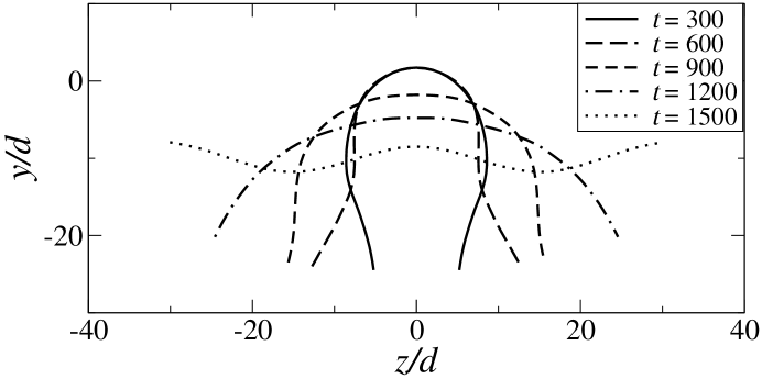
Figure 2: Filament shapes at different times: $300t_{0}$ (solid), $600t_{0}$ (long dashes), $900t_{0}$ (dashes), $1200t_{0}$ (dot dash), and $1500t_{0}$ (dotted). The time scale $t_{0}=d/c_{l}$ is the time for a longitudinal wave to cross the diameter of the filament

A straight filament of length $20\pi d$ was bent into a circle of radius $10d$ and released. The dynamics were followed for two different spatial discretizations, dividing the filament into $63$ or $127$ equal segments; the corresponding segment lengths were approximately $d$ and $0.5d$. The largest time step for the explicit integrators is Courant limited by the time, $t_{C}$, for a longitudinal wave to cross the shorter of the diameter, $d$, and the segment length, $\Delta s$; we typically use a time step $\Delta t=0.2t_{C}$. As the rod evolves from its initial configuration, flexural waves propagate along the filament, leading to a surprising variety of configurations; a sampling of the filament shapes is illustrated in Fig. 2. Initially the ends move slowly, and the filament assumes a teardrop shape ($t=300t_{0}$), followed by a hairpin ($t=600t_{0}$) as the ends of the filament accelerate. The time unit $t_{0}=d/c_{l}$, where $c_{l}$ is the longitudinal wave speed. The inverted U shape ($t=900t_{0}$) straightens out ($t=1200t_{0}$), and then develops a ”double-minimum” shape ($t=1500t_{0}$). The center of the filament moves down to complete the inversion and the filament approximately retraces the sequence of shapes in reverse order, to arrive at the inverted configuration at roughly half the period of the main oscillation. However, the motion is not exactly periodic because of the strong coupling between the flexural modes. The interaction of flexural waves can lead to large local stresses, exceeding that of the initial configuration; for example at the top of the teardrop ($t=300t_{0}$) and at the bends in the hairpin ($t=600t_{0}$). It has been shown that flexural modes can cause unexpected fractures by this mechanism.Audoly2005

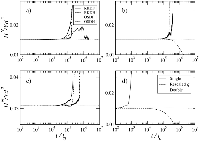
Figure 3: Conservation of energy for symplectic (OSDH) and non-symplectic (RKDF, RKDH, OSDF) algorithms. The initially circular configuration of the filament unwinds as illustrated by the snapshots in Fig. 2: a) 63 segments, $\Delta t=0.2t_{0}=0.2t_{C}$; b) 63 segments, $\Delta t=0.02t_{0}=0.02t_{C}$; c) 127 segments, $\Delta t=0.1t_{0}=0.2t_{C}$; d) OSDH algorithm with varying precision, 63 segments, $\Delta t=0.2t_{0}=0.2t_{C}$.

A complete cycle of the filament motion, back to a rough approximation of its initial configuration, takes about $6000t_{0}$ for a filament of length $L\sim 60d$, and is quadratic in the length of the filament. The scaling is due to the dispersion relation of flexural waves, $\omega\propto k^{2}$, which is quadratic rather than linear in the wavevector ($k$); the period of the longest flexural wave, $8\pi/(c_{l}k^{2}d)$ is roughly $10^{4}t_{0}$. A plot of energy vs. time, Fig. 3a, shows that all the algorithms integrate stably for about 10 oscillations, but only the symplectic methods, MPDH and OSDH, are stable at long times; on the scale of Fig. 3, results for MPDH and OSDH superpose, so only the results for OSDH are shown. We have run the MPDH and OSDH algorithms to a time of $10^{8}t_{0}$ or $16000$ periods, with no indication of instability. By contrast, changing the forces to the non-Hamiltonian form (OSDF) or switching to the RK4 integrator (RKDH) causes instabilities at times of the order of $10^{5}t_{0}$. Reducing the time step, Fig. 3b, improves the stability of the Runga-Kutta integration of the Hamiltonian forces (RKDH), increasing the range of stability by about an order of magnitude. This is because RKDH becomes symplectic in the limit $\Delta t\rightarrow 0$. On the other hand if the forces are not Hamiltonian, reducing the time step does not improve the stability; both RKDF and OSDF algorithms become unstable after a time of about $10^{5}t_{0}$, regardless of time step. The discretized forces approach a Hamiltonian form in the limit $\Delta s\rightarrow 0$ and reducing the segment length improves the stability of the OSDF algorithm, extending the range of stability by about a factor of 4 for a twofold reduction in the segment length, Fig. 3c. However, this is a double limiting process requiring a progressively smaller time step as well as a reduced segment length, making it computationally expensive. The RKDF algorithm is not helped by a reduction in segment length; it needs a further reduction in time step as well to see any improvement.

The non-linearity of the dynamics causes the filament to eventually reach a state of thermal equilibrium, fluctuating around the straight configuration. For the $63$ segment rod the equilibration time is about $10^{7}t_{0}$ independent of time step. For a constant filament length, we observe that the equilibration time is roughly quadratic in the number of segments. Thus the behavior of this system in the continuum limit is an interesting question for future work, but beyond the scope of the present paper.

The stability of the symplectic integrator is affected by accumulated round-off error. The results in Fig. 3d show that the symplectic integration scheme (OSDH) is quite unstable in single precision arithmetic. The most rapid instability, at $t<10^{3}t_{0}$, was traced to accumulated errors in the quaternion normalization. The operator splitting algorithm maintains the quaternion normalization to machine precision and with 64-bit arithmetic the normalization error is stable at less than one part in $10^{14}$. But in single precision, the error increases rapidly, which causes an incompatibility with the assumption that the nodal quaternions are normalized. More puzzling is that rescaling the quaternions does not solve the problem, but merely delays the onset of the instability. However, if the initial accumulation of round-off error is random, we would expect the double precision version to run stably for about $10^{16}$ times longer, or $10^{18}t_{0}$ which is well beyond the event horizon of the simulation.

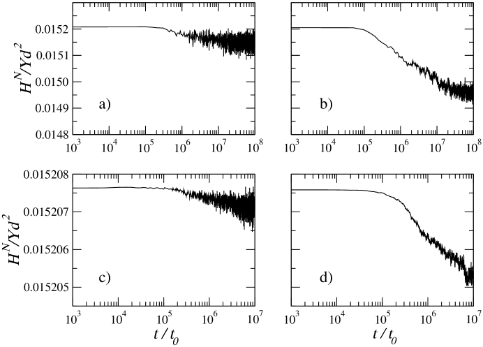
Figure 4: Conservation of energy for symplectic algorithms OSDH and MPDH; 63 segments were used in each case. a) OSDH, $\Delta t=0.2t_{0}$; b) MPDH $\Delta t=0.2t_{0}$; c) OSDH, $\Delta t=0.02t_{0}$; d) MPDH, $\Delta t=0.02t_{0}$.

The short-time fluctuations in energy of the OSDH algorithm cannot be seen on the scale of Fig. 3, but they are quadratic in the time step, with a relative magnitude of approximately $0.1(\Delta t/t_{0})^{2}$. These short-time fluctuations in energy are about 20 times larger with OSDH than with MPDH. However there is also a drift in the energy with time, again quadratic in $\Delta t$, but larger, as shown in Fig. 4. Over long time intervals, OSDH preserves energy conservation with about an order of magnitude better accuracy than MPDH at the same $\Delta t$ (Fig. 4). MPDH requires 5-10 times as many force evaluations as OSDH per time step, so that the explicit operator splitting algorithm is clearly preferable for long-time dynamics.

Dichmann and Maddocks studied the dynamics of a Kirchoff rod from the same initial configuration,Dichmann1996 but with the filament pinned at one end. The nodal forces and torques were also Hamiltonian, but the implicit midpoint integrator was used instead of operator splitting. Their results showed a small drift in the total energy of around $0.2\%$ after approximately 30 oscillations of the filament, or $200,000t_{0}$ in our units. Our results for the MPDH algorithm behave in a qualitatively similar fashion; with a time step $\Delta t=0.2t_{0}$ we observe an accumulated energy drift of $0.3\%$ at $t=200,000t_{0}$. The error with OSDH is about an order of magnitude smaller. The GE model requires a smaller time step to explicitly integrate the shear and extensional degrees of freedom, but surprisingly, it is only a factor of 8 smaller than the time step used for the constrained rod.Dichmann1996 This suggests that the explicit OSDH algorithm can integrate the full GE rod model with about the same computational cost as an implicit integration of the Kirchoff model. If excluded volume interactions are included, it is likely that these very stiff forces will set the overall time step, as is typical in molecular dynamics simulations. In such cases the computational advantages of a fully explicit simulation will be considerable.

V.2 A filament bent into a helix

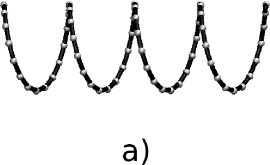
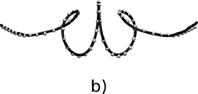
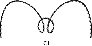
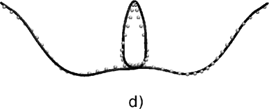
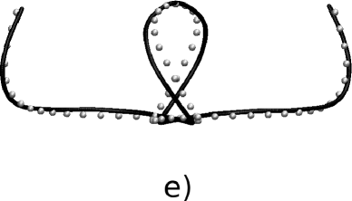
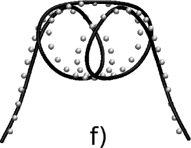
Figure 5: Filament shapes at different times: a) $t=0$; b) $t=100t_{0}$; c) $t=200t_{0}$; d) $t=300t_{0}$; e) $t=400t_{0}$; f) $t=500t_{0}$. The simulations with 630 segments are shown as thick solid lines, while simulations with 63 segments are shown by the spheres.

We have also examined a more complicated initial condition, a straight rod of length $20\pi d$ wound into a tight helix with exactly four complete turns. The curvature, ${\mbox{\boldmath${\Omega}$}}=[0.4d^{-1},0,0.1d^{-1}]$, is high and generates motion in all three spatial dimensions, which poses a difficult challenge for the numerical method. We used two different discretizations, $63$ segments of length $\Delta s\approx d$ and $630$ segments of length $\Delta s\approx 0.1d$; snapshots of the initial evolution of the filament shapes are shown in Fig. 5. There is a high degree of dynamical coherence between the results at the two different resolutions, although the strong nonlinearity of the problem means that they start to diverge at times of the order of $500t_{0}$. We did not include any excluded volume interactions in these simulations, and the filaments can therefore cross; this does not affect the accuracy of the numerical algorithm.

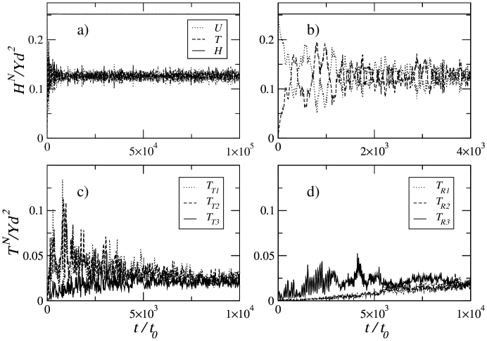
Figure 6: Conservation of energy and thermal equilibrium with the symplectic integrator OSDH. The initially helical configuration of the filament unwinds as illustrated by the snapshots in Fig. 5. The kinetic, potential and total energy of the $63$ segment model ($\Delta t=0.1t_{0}=0.1t_{C}$) are shown for: a) $10^{5}t_{0}$ and b) $4000t_{0}$. The body-fixed kinetic energy of the individual degrees of freedom is also shown: c) Shear and extension and d) Bending and torsion.

As in the planar bend case, the symplectic algorithm (OSDH) conserves energy, Fig. 6a, for as long a time as we have tested, up to $10^{6}t_{0}$. The non-linear coupling is much stronger than in the previous example, because of the higher curvature and the three-dimensional deformation; here the filament rapidly comes to thermal equilibrium. The loss of coherent oscillations can be seen more clearly in the expanded time scale of Fig. 6b. Over the same time scale, $10^{4}t_{0}$, we see that equipartition of energy is established between the various degrees of freedom, Figs. 6c and  6d; similar results holds for the various components of the potential energy as well. Unlike the planar bend case, here the more finely resolved filament ($630$ segments) comes to thermal equilibrium on more or less the same time scale, $\sim 40,000t_{0}$, rather than $10^{6}t_{0}$ as would be expected for a quadratic scaling of the equilibration time with $N$. This suggests fundamental differences in the dynamics of the two-dimensional bending from the full three-dimensional problem.

VI Conclusions

In this paper we have presented a new algorithm for simulating the dynamics of elastic filaments. The test problems show the method to be extremely stable, with exact conservation of momentum and angular momentum (to machine precision), and global energy conservation to order $\Delta t^{2}$. The algorithm is fully explicit and requires no constraints of any kind, neither on the forces nor on the quaternions. It is thus simpler in some ways than typical WLC implementations which include extensional forces as a constraint. In contrast to the WLC, the GE model correctly incorporates large bending deformations and twisting; it includes the Kirchoff rod as a limiting case.

Symplectic integration of the GE model can use a large time step, within a factor of 10 of a constrained filamentDichmann1996 that excludes shear and extensional modes. Explicit operator splitting has better long-term energy conservation than the implicit midpoint method and requires an order of magnitude fewer force evaluations per time step. In cases where the time step is limited by the stiffness of excluded volume interactions, the GE model may be more computationally efficient than the Kirchoff model, due to the absence of constraints.

In this work we only discussed Hamiltonian systems, but operator splitting is a powerful method for integrating stochastic systems as well.Serrano2006 ; Fabritiis2006 We have considered the case when the rod is subjected to dissipative and random forces, in addition to the elastic forces. Using operator splitting we can integrate the momentum equation exactly, using the Ornstein-Uhlenbeck solution, and therefore preserve quadratic norms to order $\Delta t^{2}$, as opposed to the $\Delta t$ accuracy of Brownian dynamics. This work will be reported in a future paper.

Appendix A Properties of quaternions

A quaternion ${\cal Z}=q_{0}+q_{x}i+q_{y}j+q_{z}k$ is a complex number with multiplicative identities

$$i^{2}=j^{2}=k^{2}=ijk=-1.$$ (69)

We use the notation ${\cal Z}$ to indicate the quaternion and $q_{a}$ to denote a vector containing the scalar, $q_{0}$, and vector, ${\mbox{\boldmath${q}$}}=[q_{x},q_{y},q_{z}]$, components of ${\cal Z}$. The quaternion algebra, Eq. (69), leads to rules for multiplication that are analogous to the cross-product of unit vectors:

$$ij=-ji=k$$

$$jk=-kj=i$$ (70)

$$ki=-ik=j$$

If we then identify $i$, $j$, $k$, with Cartesian unit vectors ${i}$, ${j}$, ${k}$, the multiplication of two quaternions, ${\cal Z}=q_{0}+q_{x}{\mbox{\boldmath${i}$}}+q_{y}{\mbox{\boldmath${j}$}}+q_{z}{\mbox{\boldmath${k}$}}$ and ${\cal Z}^{\prime}=q_{0}^{\prime}+q_{x}^{\prime}{\mbox{\boldmath${i}$}}+q_{y}^{\prime}{\mbox{\boldmath${j}$}}+q_{z}^{\prime}{\mbox{\boldmath${k}$}}$, can be written, using the quaternion multiplication rules defined in Eqs. 69 and 70, as

$${\cal Z}\odot{\cal Z}^{\prime}=q_{0}q_{0}^{\prime}-{\mbox{\boldmath${q}$}}\cdot{\mbox{\boldmath${q}$}}^{\prime}+q_{0}{\mbox{\boldmath${q}$}}^{\prime}+q_{0}^{\prime}{\mbox{\boldmath${q}$}}+{\mbox{\boldmath${q}$}}\times{\mbox{\boldmath${q}$}}^{\prime},$$ (71)

where $\odot$ denotes a quaternion multiplication.

A vector ${u}$ can be rotated by the unitary transformation ${\cal Z}\odot{\mbox{\boldmath${u}$}}\odot{\cal Z}^{-1}$, where the multiplicative inverse of a unit quaternion is ${\cal Z}^{-1}=q_{0}-{\mbox{\boldmath${q}$}}$. Applying Eq. 71 and treating ${u}$ as a quaternion with zero scalar component, the rotated vector ${\mbox{\boldmath${u}$}}^{\prime}$ is given by

$${\mbox{\boldmath${u}$}}^{\prime}=(q_{0}^{2}-{\mbox{\boldmath${q}$}}\cdot{\mbox{\boldmath${q}$}}){\mbox{\boldmath${u}$}}+2{\mbox{\boldmath${q}$}}{\mbox{\boldmath${q}$}}\cdot{\mbox{\boldmath${u}$}}+2q_{0}{\mbox{\boldmath${q}$}}\times{\mbox{\boldmath${u}$}},$$ (72)

and remains a pure vector. The rotation can also be written in matrix form, $u_{i}^{\prime}=d_{i\alpha}u_{\alpha}$, with the director vectors that form the rotation matrix $d_{i\alpha}$ as given in Eq. T1.2.

An infinitesimal change in the directors is given by a rotation $\delta{\mbox{\boldmath${\phi}$}}$:

$$\delta{\mbox{\boldmath${d}$}}_{i}=\delta{\mbox{\boldmath${\phi}$}}\times{\mbox{\boldmath${d}$}}_{i},$$ (73)

with ${\mbox{\boldmath${\Omega}$}}=\partial_{s}{\mbox{\boldmath${\phi}$}}$ and ${\mbox{\boldmath${\omega}$}}=\partial_{t}{\mbox{\boldmath${\phi}$}}$. The combination of the original rotation ${\cal Z}$ and an additional infinitesimal rotation $\delta{\cal Z}=1+\delta{\mbox{\boldmath${\phi}$}}/2$ can be found by applying the rotations sequentially,

$${\mbox{\boldmath${u}$}}^{\prime}+\delta{\mbox{\boldmath${u}$}}=\delta{\cal Z}\odot{\cal Z}\odot{\mbox{\boldmath${u}$}}\odot{\cal Z}^{-1}\odot\delta{\cal Z}^{-1}={\cal Z}^{\prime}\odot{\mbox{\boldmath${u}$}}\odot{\cal Z}^{\prime-1}.$$ (74)

The quaternion ${\cal Z}^{\prime}$ is found by multiplying the two quaternions,

$${\cal Z}^{\prime}=\delta{\cal Z}\odot{\cal Z}=q_{0}-{\mbox{\boldmath${q}$}}\cdot\frac{\delta{\mbox{\boldmath${\phi}$}}}{2}+{\mbox{\boldmath${q}$}}+q_{0}\frac{\delta{\mbox{\boldmath${\phi}$}}}{2}-{\mbox{\boldmath${q}$}}\times\frac{\delta{\mbox{\boldmath${\phi}$}}}{2}.$$ (75)

Thus, the variation in the quaternion $\delta{\cal Z}={\cal Z}^{\prime}-{\cal Z}$ is linearly related to $\delta{\mbox{\boldmath${\phi}$}}$,

$$\left(\begin{array}[]{c}\delta q_{0}\\ \delta q_{x}\\ \delta q_{y}\\ \delta q_{z}\end{array}\right)=\frac{1}{2}\left(\begin{array}[]{ccc}-q_{x}&-q_{y}&-q_{z}\\ ~{}~{}q_{0}&~{}~{}q_{z}&-q_{y}\\ -q_{z}&~{}~{}q_{0}&~{}~{}q_{x}\\ ~{}~{}q_{y}&-q_{x}&~{}~{}q_{0}\end{array}\right)\cdot\left(\begin{array}[]{c}\delta{\mbox{\boldmath${\phi}$}}_{x}\\ \delta{\mbox{\boldmath${\phi}$}}_{y}\\ \delta{\mbox{\boldmath${\phi}$}}_{z}\end{array}\right).$$ (76)

The column vectors in Eq. 76 define a set of basis vectors in the quaternion space, $e_{\alpha a}$, where $e_{\alpha a}$ is the transpose of the matrix in Eq. 76. These basis vectors are orthogonal to $q_{a}$ and relate changes in quaternions to rotations about the space-fixed axes,

$$\delta\phi_{\alpha}=2e_{\alpha a}\delta q_{a},~{}~{}~{}\delta q_{a}=\frac{1}{2}e_{\alpha a}\delta\phi_{\alpha}.$$ (77)

In this work we have used body-fixed rotations, Eqs. 21–22, for which we need the basis vectors $e_{ia}$ given in Eq. T1.3; they are related to the space fixed basis $e_{\alpha a}$ by the rotation matrix, $e_{ia}=d_{i\alpha}e_{\alpha a}$. The vectors $e_{ia}$ or $e_{\alpha a}$, together with $q_{a}$, form a complete basis in the quaternion space.

Finally, we obtain the derivatives of the basis vectors quoted in Eqs. T1.4–T1.5. A variation in the basis vectors ${\mbox{\boldmath${d}$}}_{i}$ is related to an infinitesimal rotation, Eq. 73,

$$\delta d_{i\alpha}=\epsilon_{\alpha\beta\gamma}\delta\phi_{\beta}d_{i\gamma}=\sum_{j,k=1}^{3}\epsilon_{ijk}d_{j\alpha}\delta\phi_{k}=2\sum_{j,k=1}^{3}\epsilon_{ijk}d_{j\alpha}e_{kb}\delta q_{b}.$$ (78)

The variation in ${\mbox{\boldmath${d}$}}_{i}$ can also be directly related to constrained variations in quaternions,

$$\delta d_{i\alpha}=\frac{\partial d_{i\alpha}}{\partial q_{a}}\left(\delta_{ab}-q_{a}q_{b}\right)\delta q_{b},$$ (79)

where the projection operator $\left(\delta_{ab}-q_{a}q_{b}\right)$ is included to ensure that the normalization condition, $\delta q_{a}q_{a}=0$, is satisfied. Equation T1.4 can then be obtained by making use of the result

$$q_{a}\frac{\partial d_{i\alpha}}{\partial q_{a}}=2d_{i\alpha}.$$ (80)

The rotation matrix can be written as a product of ${e}$ vectors, $d_{i\alpha}=e_{ia}e_{\alpha a}$. A space fixed vector is first rotated into the quaternion basis by $e_{\alpha a}/2$ and then rotated from the quaternion basis to the body-fixed frame by $2e_{ia}$. A variation in $d_{i\alpha}$ is then composed of two equal contributions from variations in $e_{ia}$ and $e_{i\alpha}$,

$$\delta d_{i\alpha}=\delta e_{ia}e_{\alpha a}+e_{ia}\delta e_{\alpha a}=2\delta e_{ia}e_{\alpha a}.$$ (81)

Substituting Eq. (78) for the variation in $d_{i\alpha}$, and using the orthogonality of the ${d}$ vectors,

$$\delta e_{ia}e_{ja}=\sum_{k=1}^{3}\epsilon_{ijk}e_{ka}\delta q_{a}.$$ (82)

Multiplying both sides by $e_{jb}$ and summing over $j$,

$$\left(\delta_{ab}-q_{a}q_{b}\right)\delta e_{ia}=\sum_{j,k=1}^{3}\epsilon_{ijk}e_{jb}e_{ka}\delta q_{a}.$$ (83)

The variation in $e_{ia}$ can also be related to constrained variations in $q_{a}$, c.f. Eq. (79), using the relation $q_{a}\delta e_{ia}=-e_{ia}\delta q_{a}$,

$$\delta e_{ia}=\frac{\partial e_{ia}}{\partial q_{c}}\left(\delta_{bc}-q_{b}q_{c}\right)\delta q_{b}=\sum_{j,k=1}^{3}\epsilon_{ijk}e_{ja}e_{kb}\delta q_{b}-q_{a}e_{ib}\delta q_{b}.$$ (84)

Equation T1.5 then follows from

$$q_{b}\frac{\partial e_{ia}}{\partial q_{b}}=e_{ia}.$$ (85)

References

• (1) J. F. Marko and E. D. Siggia, Science 265, 506 (1994).
• (2) J. F. Marko and E. D. Siggia, Phys. Rev. E 52, 2912 (1995).
• (3) D. Swigon, B. D. Coleman, and I. Tobias, Biophys. J. 74, 2515 (1998).
• (4) A. Balaeff, L. Mahadevan, and K. Schulten, Phys. Rev. Lett. 83, 4900 (1999).
• (5) B. D. Coleman, D. Swigon, and I. Tobias, Phys. Rev. E 61, 759 (2000).
• (6) I. Tobias, J. Chem. Phys. 113, 6950 (2000).
• (7) B. D. Coleman, W. K. Olson, and D. Swigon, J. Chem. Phys. 118, 7127 (2003).
• (8) V. Rossetto and A. C. Maggs, J. Chem. Phys. 118, 9864 (2003).
• (9) H. Isambert and A. C. Maggs, Europhys. Lett. 31, 263 (1995).
• (10) A. C. Maggs, Phys. Rev. E 57, 2091 (1998).
• (11) M. L. Gardel et al., Phys. Rev. Lett. 93, 188102 (2004).
• (12) B. A. DiDonna and A. J. Levine, Phys. Rev. E 75, 041909 (2007).
• (13) C. P. Brangwynne et al., J. Cell Biol. 173, 733 (2006).
• (14) W. Lawton, R. Raghavan, S. R. Ranjan, and R. Viswanathan, J. Phys. A 32, 1709 (1999).
• (15) S. Goyal, N. C. Perkins, and C. L. Lee, Int. J. Nonlin. Mech. 43, 65 (2008).
• (16) A. Goriely and S. Neukirch, Phys. Rev. Lett. 97, 184302 (2006).
• (17) J. F. Marko and E. D. Siggia, Macromolecules 27, 981 (1994).
• (18) A. J. Levine, D. A. Head, and F. C. MacKintosh, J. Phys. Cond. Mat. 16, S2079 (2004).
• (19) D. A. Head, A. J. Levine, and F. C. MacKintosh, Phys. Rev. E 72, 061914 (2005).
• (20) C. Storm, J. J. Pastore, F. C. MacKintosh, T. C. Lubensky, and P. A. Janmey, Nature 435, 191 (2005).
• (21) B. A. DiDonna and A. J. Levine, Phys. Rev. Lett. 97, 068104 (2006).
• (22) M. Das, F. C. MacKintosh, and A. J. Levine, Phys. Rev. Lett. 99, 038101 (2007).
• (23) D. Mizuno, C. Tardin, C. F. Schmidt, and F. C. MacKintosh, Science 315, 370 (2007).
• (24) F. C. MacKintosh and A. J. Levine, Phys. Rev. Lett. 100, 018104 (2008).
• (25) R. Everaers, F. Julicher, A. Ajdari, and A. C. Maggs, Phys. Rev. Lett. 82, 3717 (1999).
• (26) H. Wada and R. R. Netz, Europhys. Lett. 75, 645 (2006).
• (27) H. Wada and R. R. Netz, Europhys. Lett. 77, 68001 (2007).
• (28) I. Llopis, I. Pagonabarraga, M. C. Lagomarsino, and C. P. Lowe, Phys. Rev. E 76, 061901 (2007).
• (29) A. E. H. Love, A Treatise on the Mathematical Theory of Elasticity, Dover, fourth edition, 1944.
• (30) L. D. Landau and E. M. Lifshitz, Theory of Elasticity, Addison-Wesley, 1959.
• (31) B. D. Coleman, E. H. Dill, M. Lembo, Z. Lu, and I. Tobias, Arch. Rat. Mech. Anal. 121, 339 (1993).
• (32) I. Romero and F. Armero, Int. J. Num. Meth. Engng. 54, 1683 (2002).
• (33) T. C. Bishop, R. Cortez, and O. O. Zhmudsky, J. Comp. Phys. 193, 642 (2004).
• (34) J. C. Simo and L. Vuquoc, Comput. Meth. App. Mech. Eng. 66, 125 (1988).
• (35) J. C. Simo, N. Tarnow, and M. Doblare, Int. J. Num. Meth. Eng. 38, 1431 (1995).
• (36) S. Goyal, N. C. Perkins, and C. L. Lee, J. Comp. Phys. 209, 371 (2005).
• (37) F. Armero and I. Romero, Comp. Mech. 31, 3 (2003).
• (38) A. Dullweber, B. Leimkuhler, and R. McLachlan, J. Chem. Phys. 107, 5840 (1997).
• (39) L. Verlet, Phys. Rev. 159, 98 (1967).
• (40) T. F. Miller et al., J. Chem. Phys. 116, 8649 (2002).
• (41) R. van Zon, I. P. Omelyan, and J. Schofield, J. Chem. Phys. 128, 136102 (2008).
• (42) G. Zhong and J. E. Marsden, Phys. Lett. A 133, 134 (1988).
• (43) D. J. Dichmann and J. H. Maddocks, J. Nonlinear Sci 6, 271 (1996).
• (44) A. E. Green and N. Laws, Proc. Roy. Soc. Lond. A 293, 145 (1966).
• (45) S. Gueron and K. Levit-Gurevich, Proc. Roy. Soc. Lond. B 268, 599 (2001).
• (46) I. Klapper, J. Comp. Phys. 125, 325 (1996).
• (47) T. Y. Hou, I. Klapper, and H. Si, J. Comp. Phys. 143, 628 (1998).
• (48) A. K. Tornberg and M. J. Shelley, J. Comp. Phys. 196, 8 (2004).
• (49) J. E. Butler and E. S. G. Shaqfeh, J. Chem. Phys. 122, 014901 (2005).
• (50) D. Qi, J. Chem. Phys. 125, 114901 (2006).
• (51) L. D. Landau and E. M. Lifschitz, Mechanics, Oxford, 3rd edition, 1976.
• (52) H. Goldstein, Classical Mechanics, Addison-Wesley, 2nd edition, 1980.
• (53) R. I. McLachlan and P. Atela, Nonlinearity 5, 541 (1992).
• (54) M. Serrano, G. D. Fabritiis, P. Español, and P. Coveney, Math. Comput. Simul. 72, 190 (2006).
• (55) G. D. Fabritiis, M. Serrano, P. Español, and P. Coveney, Physica A 361, 429 (2006).
• (56) I. P. Omelyan, I. M. Mryglod, and R. Folk, Comput. Phys. Commun. 146, 188 (2002).
• (57) I. P. Omelyan, I. M. Mryglod, and R. Folk, Comput. Phys. Commun. 151, 272 (2003).
• (58) B. Audoly and S. Neukirch, Phys. Rev. Lett. 95, 095505 (2005).