A note on conductivity and charge diffusion in holographic flavor systems

Abstract:

We analyze the charge diffusion and conductivity in a $Dp/Dq$ holographic setup that is dual to a supersymmetric Yang-Mills theory in $p+1$ dimensions with $N_{f}\ll N_{c}$ flavor degrees of freedom at finite temperature and nonvanishing $U(1)$ baryon number chemical potential. We provide a new derivation of the results that generalize the membrane paradigm to the present context. We perform a numerical analysis in the particular case of the $D3/D7$ flavor system. The results obtained support the validity of the Einstein relation at finite chemical potential.

1 Introduction

The robustness of the renowned result $\eta/s=1/4\pi$ is widely thought to be related to universal properties of black hole horizons. For $p+1$-dimensional conformal field theories with a conserved charge that admit a dual holographic description a similar relation has been proposed for the diffusion constant, $D$, [1]. Recently, some understanding of how both results stated above could be derived from gravitational data that live at the black hole horizon has been pursued. In [2], by relating the charge diffusion in the boundary field theory to the analog process that occurs on the “stretched horizon” in the so called membrane paradigm, a closed analytic expression for the diffusion constant, $D$, was obtained as a a product of two factors. A local one, evaluated at the horizon, and a non-local one, involving an integral along the full range of the holographic radial direction. Certainly this smelled of holography, a point that was clarified later in [3], where the same formula was derived from a purely AdS/CFT construction. More recently [4] this factorized structure for the diffusion constant, was seen to match with the Einstein relation $D=\sigma\chi^{-1}$. In it, the conductivity $\sigma$ was given by the local factor. The other one, namely the integral along $r$, corresponded exactly to the inverse of the charge susceptibility $\chi^{-1}$, defined in equilibrium thermodynamics as the response of the charge density $n_{q}$ to a change in chemical potential $\mu$

$$\chi=\left.\frac{\partial n_{q}}{\partial\mu}\right|_{T}\,.$$ (1)

A holographic model where we can compute the above quantities in a controlled manner is naturally given by a set of $N_{f}$ “flavor” probe Dq branes, placed in the gravitational black hole background created by $N_{c}\gg N_{f}$ “color” Dp branes. In order to model a chemical potential of the boundary field theory the world-volume $U(1)$ gauge field $A_{t}$ on the probe branes has to be switched on [6, 7]. These background ingredients are enough to compute the susceptibility (1). On the other hand, both the conductivity and the diffusion constant are transport coefficients, and their computation typically involves fluctuations. From the point of view of the underlying QFT, $\sigma$ and $D$ are calculated from different channels of the retarded 2-point function of a conserved current, the transverse and longitudinal channels respectively. Up to Lorentz structures, the retarded current-current 2-point function is expressed in terms of two scalar functions $\Pi_{\perp}(k)$ and $\Pi_{||}(k)$. Fick’s law for the conserved charge density $j^{0}$ implies the existence of a universal pole in the hydrodynamic limit $k\to 0$ in $\Pi_{||}(k)$ from where the diffusive dispersion relation can be read off

$$w=-iDq^{2}+{\cal O}(q^{3})\,.$$ (2)

On the other hand, from linear response theory we can calculate the conductivity from the following static limit (see [1, 8]).

$$\sigma=-\lim_{w\to 0}\frac{{\rm Im}\Pi_{\perp}(\omega)}{\omega}\,,$$ (3)

The fact that these three quantities obey the Einstein relation $D\chi=\sigma$ provides a non-trivial consistency check of the hydrodynamic picture of holography. Also the probe approximation is consistent with it. In fact, the parametric scaling $N_{f}\ll N_{c}$ implicit in the probe approximation is correctly accounted for. Both $\chi$ and $\sigma$ arise from normalized quantities that ultimately derive from the action, and therefore show the correct scaling $N_{f}N_{c}\ll N_{c}^{2}$ with respect to bulk quantities. On the contrary $D$ stems from a pole condition and, at probe-level, does not scale with $N_{f}$. Backreaction should account for corrections of order $N_{f}/N_{c}$. This similar to the situation considered in [5] for the quotient $\eta/s$

The present paper is organized as follows. In section 2 we establish the class of models we shall be working with. In section 3 we will obtain an expression for the conductivity which includes and generalizes the one recently found in [9]. Next, in section 4, we study the charge susceptibility $\chi$, for which we also find an integral expression involving background fields that naturally extend the $n_{q}=0$ case to non-zero baryon number. Finally, in 5, we turn to the diffusion constant, $D$. First we reanalyze the case of zero baryon number, following a simplified version of the argument in [3]. After that, we turn to the full system with chemical potential. The main difficulty stems from the fact that, in computing $\Pi_{||}$, longitudinal fluctuations mix up with scalar perturbations of the probe brane profile. We prove that, unlike the case $n_{q}=0$, the diffusion constant in general is not given by the one found in [2] using the membrane paradigm. So far we are able to provide a closed expression for $D$ in terms of fluctuations, though not purely in terms of background quantities. Nevertheless, in section 6 we present numerical evidence that the Einstein relation holds also for $n_{q}\neq 0$. Assuming this is also true in general, the upshot is that the diffusion constant $D$ can be computed from background fields as $\sigma\chi^{-1}$.

2 The holographic setup

In this section we shall define the relevant notation. We will have in mind a generic holographic construction, where $N_{f}$ Dq branes are embedded in the ambient metric of $N_{c}\gg N_{f}$ Dp branes in the quenched approximation, where no backreaction of the flavor branes is taken into account. Therefore we shall parameterize a 10-dimensional metric in the form

$$ds^{2}=g_{00}(r){\rm d}x_{0}^{2}+g_{ii}(r){\rm d}\vec{x}_{p}^{2}+g_{rr}(r){\rm d}r^{2}+g_{\theta\theta}(r){\rm d}\Omega_{n}^{2}+g_{\psi\psi}(r){\rm d}\psi^{2}+g_{\varphi\varphi}(r){\rm d}\Omega_{7-p-n}^{2}\,,$$ (4)

written to simplify the notation of a Dp/Dq intersection where the probe Dq branes wrap an $n$-sphere and the transverse space is spanned by coordinates $\psi$, $\varphi^{i}$. The presence of a horizon in the background metric at $r=r_{H}$ will be encoded in the following relations

$$g_{00} = -g_{ii}(r)f(r)\,,$$

$$g_{rr} = G(r)f(r)^{-1}\,,$$

and $f(r)=(r-r_{H})F(r)$ with $F(r)$ analytic at $r=r_{H}$. The embedding of the probe brane and the $U(1)$ gauge field strength are parametrized by functions $\psi(r)$ and $A_{\mu}(r)$ respectively, whose equations of motion are derived from the Born-Infeld action

$${\cal S}_{DBI}=-N_{f}T_{Dq}\int d^{q+1}\xi e^{-\phi}\sqrt{-\det(g_{ab}+2\pi\alpha^{\prime}F_{ab})}\,.$$ (5)

The Wess-Zumino term plays no role in the following. Here we have introduced the tensor

$$\gamma_{ab}=g_{ab}+2\pi\alpha^{\prime}F_{ab}\,,$$ (6)

and we shall be interested in solutions that involve a non-zero value for the temporal component of the gauge field

$$\gamma_{0r}=2\pi\alpha^{\prime}A_{t}^{\prime}(r)=-\gamma_{r0}\,,$$ (7)

corresponding to a non-zero chemical potential. For a nonvanishing value of the gauge potential as in (7) the matrix $\gamma_{ab}$ is non-diagonal, so we list here the inverse components $\left(\gamma^{ab}\gamma_{ca}=\delta^{b}_{c}\right)$

$$\gamma_{00}=-\gamma_{ii}f(r)~{}~{};~{}~{}\gamma_{rr}=G(r)f(r)^{-1}~{}~{};~{}~{}f(r)=(r-r_{H})F(r)\,,$$

$$\gamma^{00}=\frac{\gamma_{rr}}{\gamma_{00}\gamma_{rr}+(\gamma_{0r})^{2}}~{}~{};~{}~{}\gamma^{ii}=\frac{1}{\gamma_{ii}}\,~{}~{};~{}~{}\gamma^{\theta\theta}=\frac{1}{\gamma_{\theta\theta}},$$

$$\gamma^{rr}=\frac{\gamma_{00}}{\gamma_{00}\gamma_{rr}+(\gamma_{0r})^{2}}~{}~{};~{}~{}\gamma^{0r}=-\gamma^{r0}=\frac{-\gamma_{0r}}{\gamma_{00}\gamma_{rr}+(\gamma_{0r})^{2}}\,,$$

where $\gamma_{ii}$, $\gamma_{\theta\theta}$, $\gamma_{0r}$ and $G(r)$ are regular at the horizon. The temperature can be expressed in terms of these coefficients in the near horizon limit as

$$T=\left.\frac{1}{4\pi}\frac{\gamma_{ii}f^{\prime}}{\sqrt{-\gamma_{00}\gamma_{rr}}}\right|_{r\to r_{H}}\,.$$ (8)

In general, these coefficients depend on the radial coordinate through the background profile $\psi(r)$ and the world-volume gauge field $A_{\mu}(r)$. Reduced to such degrees of freedom, and integrated along the internal unit $n$-sphere of volume $\Omega_{n}$, the $DBI$ action acquires the form

$${\cal S}_{DBI}=-N_{f}T_{Dq}\Omega_{n}\int d^{q+1-n}\xi\,e^{-\phi}\sqrt{-\left(\gamma_{00}\gamma_{rr}+\gamma_{0r}^{2}\right)\gamma_{ii}^{p}\gamma_{\theta\theta}^{n}}\,,$$ (9)

The charge density $n_{q}$ can be obtained from the electric displacement [7]

$$n_{q}=\frac{\delta{\cal S}_{DBI}}{\delta A_{t}^{\prime}(r)}=\frac{\cal N}{2\pi\alpha^{\prime}}\,e^{-\phi}\sqrt{-\gamma}\gamma^{0r}\,,$$ (10)

with $\gamma=\det\gamma_{ab}$ without the angular components of the unit $n$-sphere and ${\cal N}=N_{f}T_{D_{q}}(2\pi\alpha^{\prime})^{2}\Omega_{n}$. From the equation of motion for $A_{t}$, it follows that the charge density is independent of the radial direction, $\partial_{r}n_{q}=0$.

In the following sections we shall deal with the computation of retarded correlators. For this we consider fluctuations in the worldvolume fields of the following form

$$\psi(r,x) \to ~{}\psi(r)+\epsilon e^{-i(\omega x^{0}-qx^{1})}\Psi(r)\,,$$

$$A_{\mu}(r,x) \to A_{\mu}(r)+\epsilon e^{-i(\omega x^{0}-qx^{1})}{\cal A}_{\mu}(r)\,.$$ (11)

If we expand the Dirac-Born-Infeld lagrangian to second order in powers of $\epsilon$

$${\cal L}={\cal L}_{0}+\epsilon{\cal L}_{1}+\epsilon^{2}{\cal L}_{2}+...~{},$$ (12)

upon imposing the equations of motion for the background fields, the linear term, ${\cal L}_{1}$, vanishes identically. The linearized equations for the perturbations $\Psi$ and ${\cal A}$ are derived from the quadratic piece. In ref. [10] a detailed analysis of the retarded correlators was performed. We refer the reader to that reference for details on the equations of motion and the spectral functions.

3 The conductivity

The electrical DC conductivity may be obtained from the zero-frequency slope of the trace of the spectral function [8, 11]

$$\sigma=\left.\frac{1}{2(p-1)}\lim_{\omega\to 0}\frac{\chi^{\mu}{{}_{\mu}}(k)}{\omega}\right|_{\omega=|{\bf q}|}=\frac{1}{2p}\lim_{\omega\to 0}\frac{\chi^{\mu}{{}_{\mu}}(\omega,{\bf q}=0)}{\omega}\,.$$ (13)

The spectral function is split into two orthogonal components (see [4, 10] for notation and conventions)

$$\chi^{\mu}{{}_{\mu}}(k)=-2(p-1){\rm Im}\Pi^{\perp}(k)-2{\rm Im}\Pi^{||}(k)\,.$$ (14)

Taking into account the boundary conditions for the scalar function $\Pi^{\perp}(k)$ and $\Pi^{||}(k)$

$$\Pi_{\perp}(\omega,{\bf q}=0)=\Pi_{||}(\omega,{\bf q}=0)~{}~{}~{};~{}~{}~{}\Pi_{||}(\omega=\pm|{\bf q}|)=0\,.$$ (15)

From (13), the conductivity is uniquely obtained from the following expression

$$\sigma=-\lim_{\omega\to 0}\frac{\mathop{\rm Im}\Pi_{\perp}(\omega)}{\omega}\,,$$ (16)

independent of ${\bf q}$ (we shall confirm this independence shortly). In order to compute $\Pi_{\perp}$ we make use of the Minkowskian prescription given in [12] (see also [14]). To start with, we must solve the equations of motion for the transverse electric field fluctuations $E_{\perp}=\omega{\cal A}_{\perp}$ with ${\cal A}_{\perp}={\cal A}_{2,3}$.

$$E_{\perp}^{\prime\prime}+\partial_{r}\log\left[e^{-\phi}\sqrt{-\gamma}\gamma^{ii}\gamma^{rr}\right]E_{\perp}^{\prime}-\frac{\omega^{2}\gamma^{00}+q^{2}\gamma^{ii}}{\gamma^{rr}}E_{\perp}=0\,.$$ (17)

The horizon $r=r_{H}$ is a regular singular point, and so we may perform a Frobenius analysis. Introducing as usual the dimensionless quantities $\textswab{w}=\omega/(2\pi T)$ and $\textswab{q}=q/(2\pi T)$, the indicial exponents are found to be $\zeta_{\pm}=\pm i\textswab{w}/2$. We select $\zeta_{-}$ corresponding to incoming wave boundary conditions and set

$$E_{\perp}=f^{-i\frac{\textswab{w}}{2}}E_{\perp,reg}\,.$$ (18)

In order to analyze the solution to (17) in the hydrodynamic limit, a power counting parameter $\lambda$ is introduced. Setting $\textswab{w}\rightarrow\lambda\textswab{w}\,,~{}\textswab{q}\rightarrow\lambda\textswab{q}$ as well as

$$E_{\perp}\rightarrow f^{-i\lambda\frac{\textswab{w}}{2}}\left(E_{\perp,reg}^{(0)}+\lambda E_{\perp,reg}^{(1)}+...\right)=E_{\perp,reg}^{(0)}+\lambda\left(E_{\perp,reg}^{(1)}-i\frac{\textswab{w}}{2}E_{\perp,reg}^{(0)}\log f\right)+...$$ (19)

Expanding (17) in powers of $\lambda$ one easily solves for $E_{\perp,reg}^{(0)}(r)$ in closed form

$$E_{\perp,reg}^{(0)}(r)=C_{1}+C_{2}\int_{r_{H}}^{r}\frac{dr}{e^{-\phi}\sqrt{-\gamma}\gamma^{ii}\gamma^{rr}}\,.$$ (20)

The integrand diverges as a pole near the horizon. This enforces $C_{2}=0$ and we set $C_{1}=1$ which is simply an overall normalisation. This can then be used to solve to next order $\lambda$ in closed form

$$E_{\perp,reg}^{(1)}(r)=C_{4}\int_{C_{3}}^{r}\frac{{\rm d}r}{e^{-\phi}\sqrt{-\gamma}\gamma^{ii}\gamma^{rr}}+i\frac{\textswab{w}}{2}\log f(r)\,.$$ (21)

The logarithmic divergence at the horizon must be cancelled among the two contributions to $E_{\perp}^{(1)}(r)$ by suitably tuning $C_{4}\equiv i\textswab{w}C$, where

$$C=\left.-\frac{1}{2}e^{-\phi}\sqrt{-\gamma}\gamma^{rr}\gamma^{00}f^{\prime}\right|_{r\to r_{H}}\,.$$ (22)

The finite part is fixed by adjusting $C_{3}$ so that the boundary condition is $E_{\perp,reg}^{(1)}(r_{H})=0.$ With this

$$E_{\perp}(r)=1+i\textswab{w}\int^{r}_{C_{3}}\frac{C}{e^{-\phi}\sqrt{-\gamma}\gamma^{ii}\gamma^{rr}}{\rm d}r+{\mathcal{O}}(\textswab{w}^{2},\textswab{q}^{2})\,.$$ (23)

Once the explicit solution has been found, the on shell boundary action can be evaluated

$$S_{B}=-\frac{{\mathcal{N}}}{2}\int_{r=r_{B}}{\mathrm{d}}^{p+1}x\,e^{-\phi}\sqrt{-\gamma}\gamma^{ii}\gamma^{rr}{\cal A}^{\prime}_{\perp}{\cal A}_{\perp}\,.$$ (24)

and from it, we obtain the correlator [12]

$$\Pi_{\perp}(k)=\left.{\mathcal{N}}e^{-\phi}\sqrt{-\gamma}\gamma^{ii}\gamma^{rr}\frac{E^{\prime}_{\perp}(r)E_{\perp}(r)}{|E_{\perp}(r_{B})|^{2}}\right|_{r\to r_{B}}\,.$$ (25)

and we see from (23) that, to this order in $\lambda$, there is no dependence on $\textswab{q}$. Therefore we can write the explicit expression for the conductivity as

$$\sigma=-\frac{{1}}{2\pi T}\lim_{\textswab{w}\to 0}\frac{\mathop{\rm Im}\Pi_{\perp}(\textswab{w})}{\textswab{w}}\,.$$ (26)

In fact the imaginary part of (25) is independent of $r$, and therefore we may evaluate it at the horizon $r\to r_{H}$ rather than at $r_{B}$, because there we have explicit control over the singularities. Notice that $E_{\perp}(r)=1+{\cal O}(\textswab{w})$, so finally we obtain

$$\sigma=-{\mathcal{N}}\,\frac{C}{2\pi T}={\mathcal{N}}\,e^{-\phi}\sqrt{\gamma\gamma^{00}\gamma^{rr}}\gamma^{ii}\Bigg{|}_{r\to r_{H}}\,,$$ (27)

where use of (8) and (22) has been made. For vanishing baryon number $A_{t}=0$ the matrix $\gamma_{ab}=g_{ab}$ is diagonal and this expression fully agrees with that provided in [9]. It generalizes that result to the present context of holographic flavor systems with chemical potential.

4 The susceptibility

Let us now consider the susceptibility. This is an equilibrium quantity, given by the thermodynamical definition (1). On the one hand we have

$$\mu=A_{t}(r_{B})-A_{t}(r_{H})=\int_{r_{H}}^{r_{B}}A^{\prime}_{t}(r)dr\,,$$ (28)

since $A(r_{H})=0$ to have a well defined one-form at the horizon (see [7]). With this

$$\chi=\left(\int_{r_{H}}^{r_{B}}\frac{dA^{\prime}_{t}(r)}{dn_{q}}dr\right)^{-1}\,.$$ (29)

On the other, from (10) we can relate the charge density to $A^{\prime}_{t}(r)$

$$n_{q}={\cal N}\frac{e^{-\phi}\sqrt{H}A_{t}^{\prime}}{\sqrt{-\left(\gamma_{00}\gamma_{rr}+(2\pi\alpha^{\prime})^{2}A_{t}^{\prime 2}\right)}}\,.$$ (30)

with $H=\gamma_{ii}^{p}\gamma_{\theta\theta}^{n}$. This equation can be inverted for $A_{t}^{\prime}$ as a function of $n_{q}$

$$A_{t}^{\prime}=\frac{n_{q}}{{\cal N}}\sqrt{\frac{-\gamma_{00}\gamma_{rr}}{\displaystyle e^{-2\phi}H+\displaystyle(2\pi\alpha^{\prime})^{2}\frac{n_{q}^{2}}{{\cal N}^{2}}}}~{}.$$ (31)

Notice that in (29) we have emphasized the total derivative. This is so because on top of the explicit dependence of $A_{t}^{\prime}(r)$ on $n_{q}$, there is also a hidden one inside $\gamma_{rr}=g_{rr}+\psi^{\prime}(r)^{2}g_{\psi\psi}(\psi)$ as well as in the factor $e^{-2\phi}H=e^{-2\phi}\gamma_{ii}^{p}\gamma_{\theta\theta}^{n}$, stemming from the fact that the brane embedding $\psi(r)$ depends itself parametrically on $n_{q}$. In order to simplify (31) it is useful to make use of (10) and the following relations

$$H=\frac{\gamma}{\gamma_{00}\gamma_{rr}+\gamma_{0r}^{2}}~{}~{}~{}~{};~{}~{}~{}~{}n_{q}^{2}\frac{(2\pi\alpha^{\prime})^{2}}{{\cal N}^{2}}+e^{-2\phi}H=e^{-2\phi}\gamma\gamma^{00}\gamma^{rr}\,.$$ (32)

After some algebra one arrives at

$$\chi={\cal N}\left(\int_{r_{H}}^{r_{B}}\rule{0.0pt}{17.07164pt}\frac{1}{e^{-\phi}\sqrt{-\gamma}\gamma^{00}\gamma^{rr}}\left[1+n_{q}\left(\Delta\frac{\partial\psi^{\prime}}{\partial n_{q}}+\Xi\frac{\partial\psi}{\partial n_{q}}\right)\right]\right)^{-1}\,.$$ (33)

with

$$\Delta=\gamma^{rr}\psi^{\prime}g_{\psi\psi}~{}~{};~{}~{}\Xi=\frac{1}{2}\left(\gamma^{rr}\psi^{\prime 2}g_{\psi\psi,\psi}-n\gamma^{\theta\theta}\gamma_{\theta\theta,\psi}\right)\,.$$ (34)

It is remarkable to find the same combinations $\Delta$ and $\Xi$ that appear naturally in the equations of motion for the fluctuations (see later in (42 and ref. [10]).

5 Charge diffusion

In [2] the diffusion of a generic conserved charge was examined from the point of view of the membrane paradigm. A closed formula for this quantity was presented, and later reobtained in the context of the AdS/CFT correspondence in [3]. As a warm up exercise, we will rederive this expression in a somewhat simpler way here, first for $n_{q}=0$. The expression obtained will also be valid for $n_{q}\neq 0$ in the case of massless flavors.

5.1 Zero baryon density

The charge diffusion constant appears as a pole in the longitudinal correlator. In order to find the pole in it, one must study the equation of motion for the gauge invariant perturbations of the form $E_{||}=q{\cal A}_{0}+\omega{\cal A}_{1}$. The relevant equation of motion is

$$E_{||}^{\prime\prime}+\partial_{r}\log\left[\frac{e^{-\phi}\sqrt{-\gamma}\gamma^{ii}\gamma^{rr}}{\omega^{2}+q^{2}\frac{\gamma^{ii}}{\gamma^{00}}}\right]E_{||}^{\prime}-\frac{\omega^{2}\gamma^{00}+q^{2}\gamma^{ii}}{\gamma^{rr}}E_{||}=0\,.$$ (35)

From the diffusion pole we expect a dispersion relation of the form $\omega=-iDq^{2}+...$. Therefore the natural hydrodynamic scaling is given in terms of a variable $\lambda$ as follows $\omega\to\lambda^{2}\omega,\,q\to\lambda q$. After checking that the indices near the horizon are again $\xi_{\pm}=\pm i\textswab{w}/2$, a consistent expansion is

$$E_{||}(r)=f(r)^{-i\frac{\lambda^{2}\textswab{w}}{2}}\left(E^{(0)}_{||,reg}+\lambda^{2}E^{(2)}_{||,reg}+...\right)=E^{(0)}_{||}+\lambda^{2}E^{(2)}_{||}+...$$ (36)

Performing a Taylor expansion of the regular part around the horizon $E_{||,reg}(r)=E_{||,reg}(r_{H})+(r-r_{H})E^{\prime}_{||,reg}(r_{H})+...$ we can obtain $E^{(0)^{\prime}}_{||}(r_{H})$ solving the equation of motion (35) iteratively

$$E_{||}^{(0)}(r_{H})=1~{},~{}~{}~{}~{}E^{(0)^{\prime}}_{||}(r_{H})=-\frac{i}{2}\frac{\textswab{q}^{2}}{\textswab{w}}f^{\prime}(r_{H}).$$ (37)

Moreover, inserting the ansatz (36) into the equation of motion (35) we may solve at lowest order in closed form

$$E_{||}^{(0)}(r)=1-iC\frac{\textswab{q}^{2}}{\textswab{w}}\int_{r_{H}}^{r}\frac{{\rm d}r}{e^{-\phi}\sqrt{-\gamma}\gamma^{00}\gamma^{rr}}\,,$$ (38)

where the constant in front of the integral was fixed in accordance with (37) and (22). The relevant Green’s function is proportional to $\Pi_{||}\sim\lim_{r\to r_{B}}E_{||}^{\prime}(r)/E_{||}(r_{B})$ where the boundary is at $r_{B}$ [4]. Hence the dispersion relation comes from demanding that $E_{||}(r_{B})=0$. This provides us with the sought after dispersion relation $w=-iD_{0}q^{2}\,,$ with

$$D_{0}=\left.e^{-\phi}\sqrt{\gamma\gamma^{00}\gamma^{rr}}\gamma^{ii}\right|_{r_{H}}\int_{r_{H}}^{r_{B}}\frac{dr}{e^{-\phi}\sqrt{-\gamma}\gamma^{00}\gamma^{rr}}\,.$$ (39)

Also here, for vanishing baryon number $A_{t}=0\Rightarrow\gamma_{ab}=g_{ab}$ diagonal and (39) coincides with the one in [2].

5.2 Finite baryon density

In [13] a formula close to (39) (but not quite) was assumed to compute the value of $D_{0}$ also at finite baryon density. The influence of $n_{q}$ was supposed to show up through the dependence of the coefficients $\gamma_{ab}$ on the profile $\psi(r)$, which itself depends parametrically on the quark density. We shall see in this section that the answer that comes from examining the pole of the longitudinal propagator is more subtle.

In the presence of a background value for $A_{t}$, the longitudinal perturbations examined in the previous section mix with the scalar fluctuations on top of the probe brane profile $\Psi(r)$. The coupled set of equations of motion can be written in the following form

$$E_{||}^{\prime\prime}+{\textswab A}_{1}E_{||}^{\prime}+{\textswab B}_{1}E_{||}+{\textswab C}_{1}\Psi^{\prime\prime}+{\textswab D}_{1}\Psi^{\prime}+{\textswab E}_{1}\Psi = 0\,,$$ (40)

$$E_{||}^{\prime\prime}+{\textswab A}_{2}E_{||}^{\prime}+{\textswab B}_{2}E_{||}+{\textswab C}_{2}\Psi^{\prime\prime}+{\textswab D}_{2}\Psi^{\prime}+{\textswab E}_{2}\Psi = 0\,,$$ (41)

where the explicit form of the coefficients is reproduced from reference [10] in appendix A for completeness. From there one can easily see that all the coefficients of $\Psi$ are of order $q$. This implies that the natural variable is $\tilde{\Psi}=q\Psi$ ($\Psi$ would be natural to go with the gauge potentials ${\cal A}_{\mu}$). As before we define $\omega\to\lambda^{2}\omega,\,q\to\lambda q$ and it is clear that the coefficients of the terms multiplying $\Psi$ are all of order $\lambda$. Expanding to order $\lambda^{0}$, equation (40) becomes

$$E^{(0)^{\prime\prime}}_{||}+\log^{\prime}(\sqrt{-\gamma}\gamma^{00}\gamma^{rr})E^{(0)^{\prime}}_{||}-\frac{\gamma^{0r}}{\gamma^{00}\gamma^{rr}}\left(\Delta\tilde{\Psi}_{(0)}^{\prime}+\Xi\tilde{\Psi}_{(0)}\right)^{\prime}=0\,,$$ (42)

Using (10) this equation can be integrated to give

$$E_{||}^{(0)}=C_{1}+\int_{r_{H}}^{r}\frac{\displaystyle C_{2}+n_{q}\frac{2\pi\alpha^{\prime}}{\cal N}(\Delta\tilde{\Psi}_{(0)}^{\prime}+\Xi\tilde{\Psi}_{(0)})}{\sqrt{-\gamma}\gamma^{00}\gamma^{rr}}\,,$$ (43)

By continuity in the limit $n_{q}\to 0$ we may reasonably expect that the constants $C_{1}$ and $C_{2}$ should be the same as in the previous subsection. A more rigorous derivation comes from comparing with the Frobenius expansion around, for instance, the horizon, as we did with (37) and (38). We have performed this comparison in the specific example of the D3/D7 and found perfect agreement. Therefore we finally set

$$E_{||}^{(0)}(r)=1+\int\frac{-iC\displaystyle\frac{\textswab{q}^{2}}{\textswab{w}}+n_{q}\frac{2\pi\alpha^{\prime}}{\cal N}(\Delta\tilde{\Psi}_{(0)}^{\prime}+\Xi\tilde{\Psi}_{(0)})}{\sqrt{-\gamma}\gamma^{00}\gamma^{rr}}\,.$$ (44)

From the Dirichlet boundary condition $E_{||}^{(0)}(r_{B})=0$ we obtain the modification to the diffusion constant

$$D=\frac{D_{0}}{1+\displaystyle n_{q}\frac{2\pi\alpha^{\prime}}{{\cal N}}\int\frac{(\Delta\tilde{\Psi}_{(0)}^{\prime}+\Xi\tilde{\Psi}_{(0)})}{\sqrt{-\gamma}\gamma^{00}\gamma^{rr}}}\,.$$ (45)

The sole purpose of presenting here this rather unwieldy formula for $D$ is to emphasize that the influence of the baryon density on diffusion constant is not just given implicitely by modifying the embedding in $D_{0}$ of (39). The coupling of the scalar modes that is only present at finite density shows up as an explicit contribution. It would be nice to have an expression for $D$ in terms of purely background quantities. This would amount to an integration of the equation for the fluctuation $\Psi(r)$ which we have not achieved so far. However by providing numerical evidence that the Einstein relation holds (see section 6), we conjecture that indeed we can express $D$ as $\sigma/\chi$ where both $\sigma$ and $\chi$ are computable in terms of background quantities $A_{\mu}(r)$ and $\psi(r)$.

Still an interesting case is that of massless quarks. For such a situation $\Delta$ and $\Xi$ vanish identically, and the diffusion constant is given by $D=D_{0}$ with the dependence on $n_{q}$ coming through the dependence of $\gamma_{ab}$ on $\psi(r)$, and in this case the Einstein relation holds with finite baryon density.

6 Numerics, the D3/D7 case study

In this section we shall focus on the case of a D3/D7 flavor setup. In this particular case we call the radial coordinate $u$, with $u_{H}=1$ and $u_{B}=0$. Now $p=n=3,~{}\phi=0$ and

$$\gamma_{00}=-f(r)\frac{(\pi TL)^{2}}{u}\hskip 14.22636pt;\hskip 14.22636pt\gamma_{ii}=\frac{(\pi TL)^{2}}{u}\hskip 14.22636pt;\hskip 14.22636pt\gamma_{0u}=-2\pi\alpha^{\prime}A_{t}^{\prime}(u)$$ (46)

$$\gamma_{uu}=L^{2}\frac{1-\psi^{2}+4u^{2}f(u)\psi^{\prime 2}}{4(1-\psi^{2})u^{2}f(u)}\hskip 14.22636pt;\hskip 14.22636pt\gamma_{\theta\theta}=L^{2}(1-\psi(u)^{2})\,,$$ (47)

$$A_{t}^{\prime}(u)=-\frac{L^{2}T}{4\alpha^{\prime}}\frac{{\tilde{d}}\sqrt{1-\psi^{2}+4u^{2}f(u)\psi^{\prime 2}}}{\sqrt{(1-\psi^{2})((1-\psi^{2})^{3}+{\tilde{d}}^{2}u^{3})}}\hskip 14.22636pt\,,$$ (48)

where

$$f(u)=1-u^{2}\hskip 14.22636pt;\hskip 14.22636ptT=\frac{r_{H}}{\pi L^{2}}\,.$$ (49)

Here ${\tilde{d}}=n_{q}(2\pi\alpha^{\prime})/{\cal N}r_{H}^{3}$ is a dimensionless parameter proportional to the density, whereas the coupling reads

$${\mathcal{N}}=\frac{N_{c}N_{f}}{4\pi^{2}L^{2}}\,.$$

For finite baryon density, only results concerning the conductivity have been reliably established. In [16] a compact formula was found for the conductivity by implementing holographically Ohm’s law on a probe D7 brane. A nontrivial check of this expression was provided in [10] by using the spectral functions and the same method explained here in section 3

$$\sigma=\frac{N_{c}N_{f}T}{4\pi}\sqrt{(1-\psi_{0}^{2})^{3}+{\tilde{d}}^{2}}\,.$$ (50)

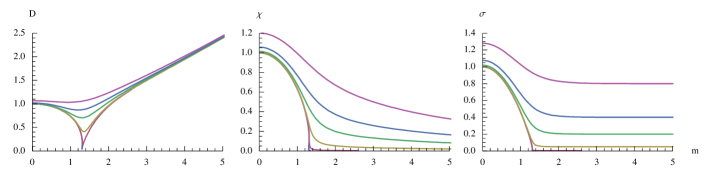
Figure 1: In this figure we plot several curves for the diffusion constant $D$ (in units of $1/2\pi T$), the susceptibility $\chi$ (in units of $N_{c}N_{f}T^{2}/2$), and the conductivity $\sigma$ (in units of $N_{c}N_{f}T/4\pi$), against the adimensional mass $m=\bar{M}/T$. From bottom to top ${\tilde{d}}=0.001,0.005,0.05,0.2,0.4$ and $0.8$.

In figure 1 we show three plots for the three quantities, $\sigma,\chi$ and $D$, appropriately scaled, for different values of the baryon density ${\tilde{d}}=0.001,0.005,0.05,0.2,0.4$ and $0.8$. They are shown as a function of the dimensionless parameter $m=\bar{M}/T$ with $\bar{M}=2M_{q}/\sqrt{\lambda}$, the mass gap. They all behave similarly, approaching different limiting values for large $m$. In the large $m$ limit, $\sigma$ approaches an $n_{q}$ dependent constant value whereas $\chi$ dies off as $\sim n_{q}/m$ and $D$ diverges proportionally to $m$ after developing a minimum close to the ${\tilde{d}}=0$ curve.

In the massless limit $m\to 0$ the diffusion constant $D$ reduces to $D_{0}$ in (39) which can be expressed in terms of a hypergeometric function [20]

$$D_{0}=\frac{1}{2\pi T}\sqrt{1+\tilde{d}^{2}}\phantom{\,}{}_{2}F_{1}\left(\frac{1}{3},\frac{3}{2};\frac{4}{3};-\tilde{d}^{2}\right)\,.$$ (51)

Figure 2: The region close to the end of the ${\tilde{d}}=0$ (blue) curve is emphasized for values of ${\tilde{d}}=0.002$, $0.00315$ and $0.004$ .

In figure 2 we have zoomed around the region of very small values of ${\tilde{d}}$. We observe the tri-valuedness that all of them exhibit for sufficiently low values of ${\tilde{d}}\leq{\tilde{d}}^{*}=0.00315$, which is related to the same property of the embeddings in this region of the parameter space [7, 13].

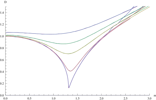
Figure 3: Comparison of the diffusion constant $D$, and the quotient $\sigma/\chi$. From bottom to top ${\tilde{d}}=0.005,0.05,0.2,0.4$ and $0.8$. We see remarkable agreement between the two calculations, up to high values of $\psi_{0}$ at which point the calculation of the excitations is subject to large numerical instabilities.

The Einstein relation

For the case of zero baryon number, the analysis performed in [4] confirmed the validity of the Einstein relation

$$D=\frac{\sigma}{\chi}\,.$$ (52)

For nonvanishing baryon number this equation holds as well in the massless limit $\psi(r)\to 0$. This can be seen from (27),(33), (39) and (45) after setting $\Xi=\Delta=0$. For massive quarks, the validity of (52) has to be established numerically. $D$ can be calculated both from a full numerical integration of (40) and (41) or by integrating $\Psi(r)$ and using (45). We found complete agreement among them. Now, plotting $D$ and $\sigma\chi^{-1}$ leads to the set of curves shown in figure 3. We find a very good agreement and the discrepancies arise for high values of $\psi_{0}\gtrsim 0.998$ where the numerical computation of $D$ is subject to large instabilities.

7 Conclusions

There is an intimate relationship between the membrane paradigm and the AdS/CFT prescription which is slowly unraveling and getting onto firmer grounds [3, 9, 18, 17]. In this short note we followed the route of the first of these citations and worked fully within the AdS/CFT context. In this way we have generalized the closed formula obtained there for the diffusion constant $D$. We have also worked out the conductivity $\sigma$ and the susceptibility $\chi$. For this last constant we provide an expression which matches the thermodynamic definition (1). An important technical detail in the calculation of $\chi$ is tracking the implicit dependence of $A_{t}^{\prime}$ on $n_{q}$ through the embedding profile $\psi(r)$ of the flavor brane. Including this contribution we have shown numerically that, at least for the D3/D7 case, the three constants obey the Einstein relation (52) also at finite baryon number $n_{q}\neq 0$. In the limit of massless quarks we have shown that this relation also holds in general.

Appendix A Coefficients for coupled longitudinal system

The coefficients that enter the system of differential equations (40) and (41) are reproduced here for completeness (see [10]).

$${\textswab A}_{1} = \log^{\prime}\left[\frac{e^{-\phi}\sqrt{-\gamma}\gamma^{ii}\gamma^{rr}}{\omega^{2}+q^{2}\frac{\gamma^{ii}}{\gamma^{00}}}\right]\,,$$ (53)

$${\textswab A}_{2} = \log^{\prime}\left[e^{-\phi}\sqrt{-\gamma}\gamma^{ii}\gamma^{rr}\right]\frac{\omega^{2}\gamma^{00}}{\omega^{2}\gamma^{00}+q^{2}\gamma^{ii}}+\frac{\Delta^{\prime}-\Xi}{\Delta}\frac{q^{2}\gamma^{ii}}{\omega^{2}\gamma^{00}+q^{2}\gamma^{ii}}\,,$$ (54)

$${\textswab B}_{1} = {\textswab B}_{2}=-\frac{\omega^{2}\gamma^{00}+q^{2}\gamma^{ii}}{\gamma^{rr}}\,,$$ (55)

$${\textswab C}_{1} = -\frac{q\,\gamma^{0r}}{\gamma^{00}\gamma^{rr}}\Delta\,,$$ (56)

$${\textswab C}_{2} = -\frac{q(1-\psi^{\prime}\Delta)}{\psi^{\prime}\gamma^{0r}}\,,$$ (57)

$${\textswab D}_{1} = -\frac{q\,\gamma^{0r}}{\gamma^{00}\gamma^{rr}}\left(\Xi+\Delta^{\prime}\right)-\frac{q\omega^{2}}{\omega^{2}\gamma^{00}+q^{2}\gamma^{ii}}\frac{\gamma^{0r}}{\gamma^{rr}}\Delta\,\log^{\prime}\left(\frac{\gamma^{ii}}{\gamma^{00}}\right)\,,$$ (58)

$${\textswab D}_{2} = -\frac{q(1-\psi^{\prime}\Delta)}{\psi^{\prime}\gamma^{0r}}\log^{\prime}\left[e^{-\phi}\sqrt{-\gamma}\gamma^{rr}g_{\psi\psi}(1-\psi^{\prime}\Delta)\right]$$ (59)

$$-\frac{\omega^{2}\gamma^{00}}{\omega^{2}\gamma^{00}+q^{2}\gamma^{ii}}\frac{q\,\gamma^{0r}}{\gamma^{00}\gamma^{rr}}\left(\log^{\prime}\left(e^{-\phi}\sqrt{-\gamma}\gamma^{ii}\gamma^{rr}\right)-\frac{\Delta^{\prime}-\Xi}{\Delta}\right)\Delta\,,$$

$${\textswab E}_{1} = -\frac{q\,\gamma^{0r}}{\gamma^{00}\gamma^{rr}}\left(\Xi^{\prime}-\Delta\frac{\omega^{2}\gamma^{00}+q^{2}\gamma^{ii}}{\gamma^{rr}}\right)-\frac{q\omega^{2}}{\omega^{2}\gamma^{00}+q^{2}\gamma^{ii}}\frac{\gamma^{0r}}{\gamma^{rr}}\Xi\,\log^{\prime}\left(\frac{\gamma^{ii}}{\gamma^{00}}\right)\,,$$ (60)

$${\textswab E}_{2} = \frac{q\,\gamma^{0r}}{\gamma^{00}\gamma^{rr}}\left[\omega^{2}\frac{\gamma^{00}}{\gamma^{rr}}\Delta-\frac{\omega^{2}\gamma^{00}}{\omega^{2}\gamma^{00}+q^{2}\gamma^{ii}}\,\Xi\left(\log^{\prime}\left(e^{-\phi}\sqrt{-\gamma}\gamma^{ii}\gamma^{rr}\right)-\frac{\Delta^{\prime}-\Xi}{\Delta}\right)\right]-\frac{q(1-\psi^{\prime}\Delta)}{\psi^{\prime}\gamma^{0r}}H(r)\,,$$

with $\Xi$ and $\Delta$ as given in (34) and $H$ (not that defined as in the main text) given here by

$$H(r) = \frac{\partial_{r}\left(e^{-\phi}\sqrt{-\gamma}\gamma^{rr}\psi^{\prime}\left(g_{\psi\psi,\psi}+\frac{n}{2}\gamma^{\theta\theta}g_{\theta\theta,\psi}g_{\psi\psi}-\frac{1}{2}\gamma^{rr}\psi^{\prime 2}g_{\psi\psi}g_{\psi\psi,\psi}\right)\right)}{e^{-\phi}\sqrt{-\gamma}\gamma^{rr}g_{\psi\psi}(1-\psi^{\prime 2}\gamma^{rr}g_{\psi\psi})}$$ (62)

$$-\frac{\left(\omega^{2}(\gamma^{00}-\psi^{\prime 2}g_{\psi\psi}(\gamma^{00}\gamma^{rr}+(\gamma^{0r})^{2}))+q^{2}\gamma^{ii}(1-\psi^{\prime 2}\gamma^{rr}g_{\psi\psi})\right)}{\gamma^{rr}(1-\psi^{\prime 2}\gamma^{rr}g_{\psi\psi})}$$

$$-\frac{\left(\frac{n(n-2)}{2}\left(\gamma^{\theta\theta}g_{\theta\theta,\psi}\right)^{2}+n\gamma^{rr}\gamma^{\theta\theta}\psi^{\prime 2}g_{\psi\psi,\psi}g_{\theta\theta,\psi}+n\gamma^{\theta\theta}g_{\theta\theta,\psi\psi}\right)}{2\gamma^{rr}g_{\psi\psi}(1-\psi^{\prime 2}\gamma^{rr}g_{\psi\psi})}$$

$$-\frac{\left(\psi^{\prime 2}g_{\psi\psi,\psi\psi}-\frac{1}{2}\gamma^{rr}\left(g_{\psi\psi,\psi}\right)^{2}\psi^{\prime 4}\right)}{2g_{\psi\psi}(1-\psi^{\prime 2}\gamma^{rr}g_{\psi\psi})}\,.$$

References

- [1] P. Kovtun and A. Ritz, “Universal conductivity and central charges,” arXiv:0806.0110 [hep-th].
- [2] P. Kovtun, D. T. Son and A. O. Starinets, “Holography and hydrodynamics: Diffusion on stretched horizons,” JHEP 0310, 064 (2003) [arXiv:hep-th/0309213].
- [3] A. O. Starinets, “Quasinormal spectrum and the black hole membrane paradigm,” arXiv:0806.3797 [hep-th].
- [4] R. C. Myers, A. O. Starinets and R. M. Thomson, “Holographic spectral functions and diffusion constants for fundamental matter,” JHEP 0711, 091 (2007) [arXiv:0706.0162 [hep-th]].
- [5] D. Mateos, R. C. Myers and R. M. Thomson, “Holographic viscosity of fundamental matter,” Phys. Rev. Lett. 98, 101601 (2007) [arXiv:hep-th/0610184].
- [6] S. Nakamura, Y. Seo, S. J. Sin and K. P. Yogendran, “A new phase at finite quark density from AdS/CFT,” J. Korean Phys. Soc. 52, 1734 (2008) [arXiv:hep-th/0611021]. “Baryon-charge Chemical Potential in AdS/CFT,” Prog. Theor. Phys. 120, 51 (2008) [arXiv:hep-th/0708.2818].
- [7] S. Kobayashi, D. Mateos, S. Matsuura, R. C. Myers and R. M. Thomson, “Holographic phase transitions at finite baryon density,” JHEP 0702, 016 (2007) [arXiv:hep-th/0611099].
- [8] S. Caron-Huot, P. Kovtun, G. D. Moore, A. Starinets and L. G. Yaffe, “Photon and dilepton production in supersymmetric Yang-Mills plasma,” JHEP 0612, 015 (2006) [arXiv:hep-th/0607237].
- [9] N. Iqbal and H. Liu, “Universality of the hydrodynamic limit in AdS/CFT and the membrane paradigm,” arXiv:0809.3808 [hep-th].
- [10] J. Mas, J. P. Shock, J. Tarrio and D. Zoakos, “Holographic Spectral Functions at Finite Baryon Density,” JHEP 0809, 009 (2008) [arXiv:0805.2601 [hep-th]].
- [11] D. Mateos and L. Patiño, JHEP 0711, 025 (2007) [arXiv:0709.2168 [hep-th]].
- [12] D. T. Son and A. O. Starinets, “Minkowski-space correlators in AdS/CFT correspondence: Recipe and applications,” JHEP 0209, 042 (2002) [arXiv:hep-th/0205051].
- [13] J. Erdmenger, M. Kaminski, P. Kerner and F. Rust, “Finite baryon and isospin chemical potential in AdS/CFT with flavor,” arXiv:0807.2663 [hep-th].
- [14] P. K. Kovtun and A. O. Starinets, “Quasinormal modes and holography,” Phys. Rev. D 72, 086009 (2005) [arXiv:hep-th/0506184].
- [15] D. T. Son and A. O. Starinets, “Hydrodynamics of R-charged black holes,” JHEP 0603, 052 (2006) [arXiv:hep-th/0601157].
- [16] A. Karch and A. O’Bannon, “Metallic AdS/CFT,” JHEP 0709, 024 (2007) [arXiv:0705.3870 [hep-th]].
- [17] M. Fujita, “Non-equilibrium thermodynamics near the horizon and holography,” JHEP 0810, 031 (2008) [arXiv:0712.2289 [hep-th]].
- [18] R. Brustein and A. J. M. Medved, “The shear diffusion coefficient for generalized theories of gravity,” arXiv:0810.2193 [hep-th].
- [19] D. Mateos, S. Matsuura, R. C. Myers and R. M. Thomson, “Holographic phase transitions at finite chemical potential,” JHEP 0711, 085 (2007) [arXiv:0709.1225 [hep-th]].
- [20] K. Y. Kim and I. Zahed, “Baryonic Response of Dense Holographic QCD,” arXiv:0811.0184 [hep-th].