Spin Orientation of Holes in Quantum Wells

Abstract

This article reviews the spin orientation of spin-3/2 holes in quantum wells. We discuss the Zeeman and Rashba spin splitting in hole systems that are qualitatively different from their counterparts in electron systems. We show how a systematic understanding of the unusual spin-dependent phenomena in hole systems can be gained using a multipole expansion of the spin density matrix. As an example we discuss spin precession in hole systems that can give rise to an alternating spin polarization. Finally we discuss the qualitatively different regimes of hole spin polarization decay in clean and dirty samples.

I Introduction

Spin electronics is a quickly developing research area that has yielded considerable new physics and the promise of novel applications wol01 . The electrons in the conduction band of common semiconductors like GaAs are characterized by a spin-1/2. Holes in the topmost valence band, on the other hand, have an effective spin-3/2 (Ref. lut56 ) which gives rise to many novel features that are not present in the conceptually simpler case of spin-1/2 electron systems.

In this article we review some of the intriguing phenomena related with the spin orientation in spin-3/2 hole systems. We begin in Sec. II with a brief review of the Luttinger Hamiltonian which forms the foundation for a theoretical description of spin-3/2 hole systems in cubic semiconductors like GaAs. In Sec. III we discuss the anisotropic Zeeman splitting of two-dimensional (2D) hole systems. While a magnetic field $B$ perpendicular to the 2D plane gives rise to a large Zeeman splitting, the splitting in an in-plane magnetic field is greatly suppressed. However, it can be tuned, e.g., by varying the thickness of the quasi-2D system by means of external gates. At $B=0$, the Rashba spin-orbit coupling in an inversion-asymmetric 2D system is characterized by an effective magnetic field oriented in the 2D plane. As discussed in Sec. IV, the resulting spin splitting in 2D hole systems behaves thus very similar to the Zeeman splitting in an external magnetic field. In particular, Rashba spin splitting can likewise be tuned by varying the thickness of the quasi-2D system.

In Sec. V we review the multipole expansion of the spin density matrix that provides a more systematic understanding of the unusual spin-dependent phenomena in hole systems. As a first application of this general approach, we discuss in Sec. VI the multipole moments induced in a 2D hole system by an in-plane magnetic field. Next we use the multipole expansion to discuss in Sec. VII the spin precession in 2D hole systems which turns out to be qualitatively different from the more familiar case of spin precession in spin-3/2 hole systems. For example, the hole spin polarization and the higher-order multipoles can precess due to the spin-orbit coupling in the valence band, yet in the absence of external or effective magnetic fields. Finally, we discuss in Sec. VIII the spin polarization decay in hole systems. Here, an important parameter is the product of the precession frequency $\Omega$ times the momentum relaxation time $\tau_{p}$. Qualitatively different regimes can be distinguished for dirty samples with $\Omega\tau_{p}\ll 1$, weak-scattering samples with $\Omega\tau_{p}\gg 1$ and ballistic systems with $\tau_{p}\rightarrow\infty$. In Sec. IX we summarize our results.

II Spin-3/2 Hole Systems: the Luttinger Hamiltonian

In a tight-binding picture, the electrons in the conduction band of common semiconductors like GaAs are described by $s$-like atomic orbitals yu01 ; win03 , see Fig. 1 (left). Taking into account spin, the electrons have a total angular momentum $j=1/2$ that behaves analogously to a spin $s=1/2$. Holes, on the other hand, are described by $p$-like atomic orbitals. Taking into account spin, the holes have a total angular momentum $j=3/2$ and $j=1/2$. The atomic spin-orbit coupling separates the $j=3/2$ from the $j=1/2$ states by a spin-orbit gap $\Delta_{0}$, see Fig. 1 (center), so that we can associate an effective spin $j=3/2$ with the states in the topmost valence band. At nonzero wave vectors $k$ the fourfold degenerate states $j=3/2$ split further into so-called heavy-hole (HH) and light-hole (LH) states. If we choose the quantization axis of angular momentum ${\bm{\mathrm{j}}}$ parallel to ${\bm{\mathrm{k}}}$, the HH (LH) states corresponds to $m=\pm 3/2$ ($m=\pm 1/2$). (We ignore here small $k$-linear terms that couple HH and LH states lut56 .)

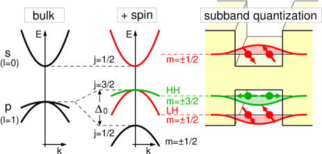
Figure 1: Qualitative sketch of the band structure of GaAs close to the fundamental gap. (Left) The electrons in the conduction band are described by $s$-like atomic orbitals whereas the holes in the the topmost valence band are described by $p$-like atomic orbitals. (Center) Taking into account spin, the conduction band states are characterized by a total angular moment $j=1/2$, whereas in the valence band we have $j=3/2$ and $j=1/2$ states seperated by a spin-orbit gap $\Delta_{0}$. (Right) In quasi-2D systems the $j=3/2$ states split into HH and LH states. For electron and LH states the spin is essentially decoupled from the orbital motion, whereas HH states are predominantly made of $m=\pm 3/2$ states with a spin quantization axis perpendicular to the 2D plane.

In the following we consider quasi two-dimensional (quasi-2D) systems in the $xy$ plane. Subband quantization in quasi-2D systems correspond to standing waves in the $z$ direction so that we get a splitting of HH and LH states called the HH-LH splitting, even for in-plane wave vector $k_{\|}=0$, see Fig. 1 (right). For 2D systems grown on a high-symmetry (001) or (111) surface, the $k_{\|}=0$ eigenstates are pure HH or LH eigenstates (if we neglect the small $k$-linear terms). For any other surface, e.g., the experimentally important (113) surface dav91 ; her94 , we obtain a weak coupling of HH and LH states even at $k_{\|}=0$ which is caused by the terms of cubic symmetry in the Hamiltonian (see below).

For $k_{\|}\neq 0$ we get a mixing of HH and LH states. However, for typical sample parameters (well width and Fermi wave vector $k_{F}$), the wave vector $k_{z}$ characterizing the standing wave perpendicular to the 2D plane is generally much larger than $k_{F}$, $k_{z}\gg k_{F}$, so that we can interpret the subband states even for $k_{\|}\neq 0$ as HH or LH-like. Often, only the lowest HH subband is occupied, i.e., the occupied subband states are predominantly made of $m=\pm 3/2$ states assuming a spin quantization axis perpendicular to the 2D plane. It is this fact that lies at the heart of several anomalous properties of 2D hole systems that we are going to discuss in subsequent sections. Of course, at magnetic field $B=0$ the $m=+3/2$ and $m=-3/2$ states contribute with equal weight, i.e., as expected for a paramagnetic material, the effects discussed here do not give rise to a permanent magnetic moment.

For a more explicit and detailed discussion of spin orientation we need to use the Hamiltonian appropriate for these hole systems. Generally, the $j=3/2$ hole states in the topmost valence band of cubic semiconductors like GaAs are described by the Luttinger Hamiltonian lut56

$$\begin{array}[b]{r@{}l}\mathcal{H}_{L}=\displaystyle-\frac{\hbar^{2}}{2m_{0}}\bigl{\{}\gamma_{1}k^{2}&{}-2\gamma_{2}\left[\left(J_{x}^{2}-{\textstyle\frac{1}{3}}J^{2}\right)k_{x}^{2}+\mathrm{cp}\right]\\[4.30554pt] &{}-4\gamma_{3}\left[\left\{J_{x},J_{y}\right\}k_{x}k_{y}+\mathrm{cp}\right]\bigr{\}},\end{array}$$ (1)

where $m_{0}$ is the mass of free electrons, $\gamma_{1}$, $\gamma_{2}$, and $\gamma_{3}$ are the Luttinger parameters, $J_{i}$ are the $4\times 4$ matrices for angular momentum $j=3/2$ (see, e.g., Ref. win03 ), we have $\{A,B\}=\frac{1}{2}(AB+BA)$ and cp denotes cyclic permutation. In Eq. (1) we neglected the terms linear and cubic in $k$ which contribute to the spin splitting due to bulk inversion asymmetry win03 . We remark that for the effects discussed here these terms are of minor importance. Using an explicit matrix notation, $\mathcal{H}_{L}$ can be written in the form bal70

$$\mathcal{H}_{L}=\left(\begin{array}[]{cccc}P+Q&L&M&0\\ L^{\ast}&P-Q&0&M\\ M^{\ast}&0&P-Q&-L\\ 0&M^{\ast}&-L^{\ast}&P+Q\end{array}\right),$$ (2)

where

$$P = -\frac{\hbar^{2}}{2m_{0}}\,\gamma_{1}\,k^{2}$$ (3a)

$$Q = \frac{\hbar^{2}}{2m_{0}}\,\gamma_{2}\,(2k_{z}^{2}-k_{x}^{2}-k_{y}^{2})$$ (3b)

$$L = \frac{\hbar^{2}}{2m_{0}}\,2\sqrt{3}\gamma_{3}\,(k_{x}-ik_{y})k_{z}$$ (3c)

$$M = \frac{\hbar^{2}}{2m_{0}}\,\sqrt{3}\left[\gamma_{2}(k_{x}^{2}-k_{y}^{2})-2i\gamma_{3}\,k_{x}k_{y}\right].$$ (3d)

Here we have expressed $J_{i}$ and $\mathcal{H}_{L}$ in a basis of $j=3/2$ angular momentum eigenfunctions in the order $m=+3/2$, $+1/2$, $-1/2$, and $-3/2$.

The notation used in Eq. (1) reflects the cubic symmetry of the crystal structure. An alternative formulation of the Luttinger Hamiltonian was proposed by Lipari and Baldereschi lip70

$$\mathcal{H}_{L}=-\frac{\hbar^{2}}{2m_{0}}\gamma_{1}k^{2}-\frac{\hbar^{2}}{2m_{0}}\bar{\gamma}\left[{\textstyle\frac{5}{2}}k^{2}-2({\bm{\mathrm{k}}}\cdot{\bm{\mathrm{J}}})^{2}\right]+\mathcal{H}_{\mathrm{c}},$$ (4)

where $\bar{\gamma}\equiv(2\gamma_{2}+3\gamma_{3})/5$ and ${\bm{\mathrm{J}}}=(J_{x},J_{y},J_{z})$. The first two terms in Eq. (4) have spherical symmetry with the first term being diagonal in spin while the second term can be interpreted as a spherical spin-orbit coupling within the $j=3/2$ space, see also Eq. (19) below. Finally, $\mathcal{H}_{\mathrm{c}}$ represents the anisotropic terms with cubic symmetry lip70 which will be given in Eq. (20) below. Usually the terms in $\mathcal{H}_{\mathrm{c}}$ are small. Neglecting these terms corresponds to the spherical approximation $\mathcal{H}_{s}$ of $\mathcal{H}_{L}$. Using for $\mathcal{H}_{s}$ an explicit matrix notation as in Eq. (2) we get $P_{s}=P$ and

$$Q_{s} = \frac{\hbar^{2}}{2m_{0}}\,\bar{\gamma}\,(2k_{z}^{2}-k_{x}^{2}-k_{y}^{2})$$ (5a)

$$L_{s} = \frac{\hbar^{2}}{2m_{0}}\,2\sqrt{3}\bar{\gamma}\,k_{-}k_{z}$$ (5b)

$$M_{s} = \frac{\hbar^{2}}{2m_{0}}\,\sqrt{3}\bar{\gamma}\,k_{-}^{2},$$ (5c)

where $k_{\pm}\equiv k_{x}\pm ik_{y}$. In the spherical approximation, the energy dispersions for the HH and LH states are

$$E_{\mathrm{LH/HH}}({\bm{\mathrm{k}}})=-\frac{\hbar^{2}}{2m_{0}}\,(\gamma_{1}\pm 2\bar{\gamma})\>k^{2}.$$ (6)

For quasi-2D systems it is often advantageous to use an alternative decomposition $\mathcal{H}_{L}=\mathcal{H}_{\mathrm{ax}}+\mathcal{H}_{\mathrm{c}}^{\prime}$, where $\mathcal{H}_{\mathrm{ax}}$ has axial symmetry with the symmetry axis ${\bm{\mathrm{n}}}$ chosen perpendicular to the 2D plane. Neglecting $\mathcal{H}_{\mathrm{c}}^{\prime}$ corresponds to the axial approximation tre79 ; win03 . For ${\bm{\mathrm{n}}}$ parallel to $[001]$ we obtain for $\mathcal{H}_{\mathrm{ax}}$, using an explicit matrix notation as in Eq. (2),

$$P_{\mathrm{ax}} = P,\qquad Q_{\mathrm{ax}}=Q,\qquad L_{\mathrm{ax}}=L$$ (7a)

$$M_{\mathrm{ax}} = \frac{\hbar^{2}}{2m_{0}}\,\sqrt{3}\,\frac{\gamma_{2}+\gamma_{3}}{2}\,k_{-}^{2}.$$ (7b)

Explicit expressions for other crystallographic orientations of ${\bm{\mathrm{n}}}$ are given in Refs. tre79 ; win03 . For quasi-2D systems the advantage of the axial approximation over the spherical approxiamtion lies in the fact that $\mathcal{H}_{\mathrm{ax}}$ captures the most important physics of different crystallographic directions ${\bm{\mathrm{n}}}$ while both $\mathcal{H}_{\mathrm{s}}$ and $\mathcal{H}_{\mathrm{ax}}$ yield a rotational symmetry with respect to the axis ${\bm{\mathrm{n}}}$.

We can readily see from Eq. (2) that $\mathcal{H}_{L}$ becomes diagonal for $k_{x}=k_{y}=0$, i.e., subband states at $k_{\|}=0$ are either pure HH ($m=\pm 3/2$) or pure LH ($m=\pm 1/2$) states. As discussed above, in a coordinate frame where the $z$ axis points in a crystallographic direction other than the high-symmetry directions [001] or [111], $\mathcal{H}_{L}$ contains off-diagonal terms proportional to $k_{z}^{2}$ so that even at the subband edge $k_{\|}=0$ we get a mixing of HH and LH states.

III Anisotropic Zeeman Splitting

For spin-1/2 electron systems it is well-known that the Zeeman splitting, i.e., the response of the electron’s spin to a magnetic field ${\bm{\mathrm{B}}}$, is usually essentially independent of the orientation of ${\bm{\mathrm{B}}}$ fan68 . For electrons, the differences between the in-plane and perpendicular effective Landé factors $g^{\ast}_{\|}$ and $g^{\ast}_{\perp}$ are most pronounced in narrow GaAs-AlGaAs quantum wells, where $g^{\ast}_{\|}$ and $g^{\ast}_{\perp}$ change sign and thus cross zero as a function of well width, as discussed in Refs. ivc92 ; kal92 . The in-plane anisotropy of the in-plane $g^{\ast}_{\|}$ in low-symmetry geometries was discussed in Ref. kal93 , see also Ref. win03 .

The situation in HH systems is qualitatively different. As suggested by Fig. 1, the response of a HH system to an in-plane magnetic field $B_{\|}$ is suppressed because the effect of $B_{\|}$ competes with the rather rigid spin orientation induced by the HH-LH splitting. A perpendicular magnetic field $B_{\perp}$, on the other hand, is compatible with the $B=0$ spin orientation of the $m=\pm 3/2$ HH states so that we can have a large Zeeman splitting. The resulting anisotropy of $g^{\ast}$ was first discussed in Ref. kes90 .

A more quantitative discussion needs to be based on the Luttinger Hamiltonian $\mathcal{H}_{L}$ with the Zeeman term $\mathcal{H}_{Z}=-2\mu_{\mathrm{B}}\,\kappa\,{\bm{\mathrm{B}}}\cdot{\bm{\mathrm{J}}}$ added to it. Here $\kappa$ is the isotropic $g$ factor. We neglect the anisotropic Zeeman term because its prefactor (often denoted $q$ lut56 ) is usually much smaller than $\kappa$. Using an explicit matrix notation, the Zeeman term reads

$$\mathcal{H}_{Z}=-2\kappa\mu_{\mathrm{B}}\left(\!\begin{array}[]{cccc}\frac{3}{2}B_{z}&\frac{\sqrt{3}}{2}B_{-}&0&0\\ \frac{\sqrt{3}}{2}B_{+}&\frac{1}{2}B_{z}&B_{-}&0\\ 0&B_{+}&-\frac{1}{2}B_{z}&\frac{\sqrt{3}}{2}B_{-}\\ 0&0&\frac{\sqrt{3}}{2}B_{+}&-\frac{3}{2}B_{z}\end{array}\!\right),$$ (8)

where $B_{\pm}\equiv B_{x}\pm iB_{y}$. We can immediately read off from Eq. (8) that a perpendicular magnetic field $B_{z}$ gives rise to a Zeeman splitting $\Delta E_{\mathrm{HH}}=6\mu_{\mathrm{B}}\kappa B_{z}$ of the HH states whereas for LH states we get $\Delta E_{\mathrm{HH}}=2\mu_{\mathrm{B}}\kappa B_{z}$. Also, we see from Eq. (8) that, in the presence of an in-plane magnetic field ${\bm{\mathrm{B}}}_{\|}=(B_{x},B_{y},0)$, the Zeeman term $\mathcal{H}_{Z}$ couples the two LH states with $\Delta E_{\mathrm{LH}}=4\mu_{\mathrm{B}}\kappa B_{\|}$, and it couples the HH states to the LH states gol93 . But there is no direct coupling between the HH states proportional to $\kappa$, so that the Zeeman splitting of HH states in an in-plane magnetic field is suppressed kes90 .

A quantitative analysis based on perturbation theory shows win03 that, for $k_{\|}=0$ and neglecting the cubic terms $\mathcal{H}_{\mathrm{c}}$, there is no Zeeman splitting of HH states linear in $B_{\|}$, but the lowest-order splitting is proportional to $B_{\|}^{3}$

$$\Delta E_{Z\|}\propto\frac{B_{\|}^{3}}{\Delta_{11}^{hl}},$$ (9a)

where $$\Delta_{\lambda\lambda^{\prime}}^{\nu\nu^{\prime}}\equiv E_{\lambda}^{\nu}-E_{\lambda^{\prime}}^{\nu^{\prime}} E_{\lambda}^{h} E_{\lambda}^{l} \lambda k_{\|}>0$$ with and the energy of the th HH and LH subband, respectively. Similarly, we obtain for

$$\Delta E_{Z\|}\propto\frac{k_{\|}^{2}\,B_{\|}}{\Delta_{11}^{hl}}.$$ (9b)

As expected from Fig. 1, the energy denominators in Eq. (9) reflect the competition between the spin orientation perpendicular to the 2D plane induced by the subband confinement and the (generally weaker) effect of the in-plane magnetic field $B_{\|}$ that tends to orient the spins in-plane. The $k_{\|}$ dependence in Eq. (9b) originates in the HH-LH coupling at $k_{\|}>0$. It follows from Eq. (9) that we can tune the Zeeman splitting of HH systems in an in-plane magnetic field if we change the confinement in $z$ direction by means of front and/or back gates. Alternatively, one can also change the HH-LH splitting by means of strain.

When taking into account the cubic terms $\mathcal{H}_{\mathrm{c}}$ in the Luttinger Hamiltonian, the Zeeman splitting linear in $B_{\|}$ ($k_{\|}=0$) still vanishes for the high-symmetry surfaces (001) and (111). For other surfaces, we get a $B_{\|}$-linear splitting the magnitude of which depends on the in-plane orientation of ${\bm{\mathrm{B}}}_{\|}$ relative to the crystal axes win00b . For an infinitely deep rectangular QW grown on an $(mmn)$ surface we obtain in second order perturbation theory the following Zeeman terms acting within the space of the topmost HH subband

$$\mathcal{H}^{\mathrm{HH}}_{[mmn]}=\frac{\mu_{\mathrm{B}}}{2}\left(g_{xx}^{\ast}B_{x}\sigma_{x}+g_{xz}^{\ast}B_{x}\sigma_{z}+g_{yy}^{\ast}B_{y}\sigma_{y}\right)$$ (10a)

where

$$g_{xx}^{\ast} = g_{yy}^{\ast}=-6\mathcal{K}\left(2-3\sin^{2}\theta\right)\sin^{2}\theta$$ (10b)

$$g_{xz}^{\ast} = 12\mathcal{K}\left(2-3\sin^{2}\theta\right)\sin\theta\cos\theta$$ (10c)

Here the $x$ direction corresponds to $[nn\overline{(2m)}]$, $y$ corresponds to $[\overline{1}10]$ and $\theta$ is the angle between $[mmn]$ and $[001]$, i.e. $\theta=\arccos(n/\sqrt{2m^{2}+n^{2}})$. We obtain for the coefficient $\mathcal{K}$

$$\mathcal{K}=\frac{\kappa(\gamma_{3}-\gamma_{2})}{4\left[\left(1-\zeta\right)\gamma_{2}+\zeta\gamma_{3}\right]}$$ (11a)

where

$$\zeta=\sin^{2}\theta\left[3-{\textstyle\frac{9}{4}}\sin^{2}\theta\right].$$ (11b)

Note that these expressions are independent of the width of the QW. The importance of Eq. (10) lies in the fact that the topmost subband in an (unstrained) QW is an HH subband so that often only this subband is occupied. In Fig. 2 we show $g_{xx}^{\ast}=g_{yy}^{\ast}$ and $g_{xz}^{\ast}$ for the topmost HH subband in a GaAs–AlGaAs QW as a function of the angle $\theta$. Figure 2 demonstrates that $g^{\ast}$ can be very anisotropic. For example, for the growth direction [113], $g^{\ast}_{xz}$ is more than a factor of four larger than $g_{xx}^{\ast}=g_{yy}^{\ast}$. For comparison, we remark that for the GaAs system considered in Fig. 2 we have $g_{zz}^{\ast}=6\kappa\approx 7.2$. Equations (10) and (11) are applicable to a wide range of cubic semiconductors with results qualitatively very similar to Fig. 2.

Figure 2: Anisotropic effective $g$ factor $g^{\ast}$ of the $h_{1}$ subband for a GaAs–AlGaAs QW as a function of $\theta$, the angle between [001] and the growth direction. Here $\hat{{\bm{\mathrm{x}}}}\parallel[nn\overline{(2m)}]$, $\hat{{\bm{\mathrm{y}}}}\parallel[\bar{1}10]$ and $\hat{{\bm{\mathrm{z}}}}\parallel[mmn]$.

The anisotropic Zeeman splitting (10) has been studied experimentally by measuring the magnetoresistance of a high-mobility 2D hole system as a function of in-plane magnetic field $B_{\|}$ win00b . The sample was a 200 Å wide Si-modulation doped GaAs QW grown on (113)A GaAs substrate. The left two panels of Fig. 3 show the resistivity $\rho$ measured as a function of $B_{\|}$ for different directions of ${\bm{\mathrm{B}}}_{\|}$ and current ${\bm{\mathrm{I}}}$ and for three different densities. For easier comparison we have plotted the fractional change $\rho(B_{\|})/\rho(0)$. It can be seen that $\log(\rho)$ shows a change in slope at a value of $B_{\|}$ we call $B^{\ast}$. In Fig. 3 $B^{\ast}$ is marked by arrows. This magnetoresistance feature is related to a spin-subband depopulation and the resulting changes in subband mobility and intersubband scattering as $B_{\|}$ is increased oka99 ; pap00a . It is remarkable that $B^{\ast}$ for the ${\bm{\mathrm{B}}}\parallel[33\bar{2}]$ traces is several Tesla smaller than for the $[\bar{1}10]$ traces, but it is independent of the direction of ${\bm{\mathrm{I}}}$. This is strong evidence for the anisotropy of the in-plane $g^{\ast}$. The experimentally observed anisotropy is qualitatively consistent with our self-consistently calculated results for the density $p_{+}$ of the upper spin subband as a function of $B_{\|}$, shown in the right panel of Fig. 3. The density $p_{+}$ decreases much faster for ${\bm{\mathrm{B}}}\parallel[33\bar{2}]$ than for ${\bm{\mathrm{B}}}\parallel[\bar{1}10]$, in agreement with Fig. 2. The findings have been confirmed by Shubnikov-de Haas measurements probing directly the depopulation of the minority spin subband for different orientations of ${\bm{\mathrm{B}}}_{\|}$ tut01 .

Figure 3: Left and central panels: Fractional change in resistivity $\rho(B_{\|})/\rho(0)$ due to an in-plane $B$, measured at $T=0.3$ K in a GaAs 2D hole system grown on a (113) substrate, for different directions of ${\bm{\mathrm{B}}}_{\|}$ and ${\bm{\mathrm{I}}}$ and different 2D densities as indicated. The arrows mark $B^{\ast}$ as defined in the text. Right panel: Calculated density $p_{+}$ in the upper spin subband as a function of $B_{\|}$.

In Fig. 3 the measured $B^{\ast}$ is significantly smaller than the calculated $B_{\|}$ for a complete depopulation of the upper spin-subband. We note that for our low-density samples it can be expected that $g^{\ast}$ is enhanced due to the exchange interaction and the spin polarization caused by $B_{\|}$ fan68 ; kwo94 ; oka99 . These many-particle effects were not taken into account in our self-consistent calculations. However, they do not qualitatively affect the anisotropy of $g^{\ast}$ win00b . See Ref. win05 for a more detailed discussion of exchange-correlation effects in low-density hole systems on a (113) surface.

IV Rashba Spin Splitting in 2D Hole Systems

If in a solid the spatial inversion symmetry is broken, we can have a spin splitting of the electron and hole states even in the absence of a magnetic field $B$. In quasi-2D semiconductor structures, the bulk inversion asymmetry (BIA) of the underlying crystal structure (e.g., a zinc blende structure), and the structure inversion asymmetry (SIA) of the confining potential are usually the dominant contributions to the $B=0$ spin splitting ros89 . While BIA is fixed, the so-called Rashba spin splitting byc84 due to SIA can be tuned by means of external gates that change the electric field $\mathcal{E}$ in the sample nit97 ; pap99 .

Here we want to focus on Rashba spin splitting. In quasi-2D electron systems it is described by the term

$$\mathcal{H}_{R}^{\mathrm{e}}=\alpha\mathcal{E}_{z}i\left(k_{-}\sigma_{+}-k_{+}\sigma_{-}\right)=\alpha\mathcal{E}_{z}\left(\begin{array}[]{cc}0&ik_{-}\\ -ik_{+}&0\end{array}\right)\,,$$ (12)

where $\sigma_{\pm}\equiv\frac{1}{2}(\sigma_{x}\pm i\sigma_{y})$, $\alpha$ is a material-dependent prefactor and $\mathcal{E}_{z}$ is an (effective) electric field that characterizes the broken inversion symmetry of the sample. Often it is instructive to write the Rashba term (12) in the form of a Zeeman term win04

$$\mathcal{H}_{R}^{\mathrm{e}}={\textstyle\frac{1}{2}}\>{\bm{\mathcal{B}}}({\bm{\mathrm{k}}}_{\|})\cdot{\bm{\mathrm{\sigma}}}$$ (13)

where ${\bm{\mathcal{B}}}({\bm{\mathrm{k}}}_{\|})=2\alpha\mathcal{E}_{z}(k_{y},-k_{x},0)$ is an effective magnetic field. It follows from the defintion of ${\bm{\mathcal{B}}}({\bm{\mathrm{k}}}_{\|})$ that ${\bm{\mathcal{B}}}$ orients the electron spin in the plane of the 2D structure, perpendicular to the wave vector ${\bm{\mathrm{k}}}_{\|}$.

For $j=3/2$ hole systems we need to replace the $2\times 2$ Pauli matrices $\sigma_{x}$ and $\sigma_{y}$ in Eq. (12) or (13) by the corresponding $4\times 4$ matrices $J_{x}$ and $J_{y}$ for angular momentum $j=3/2$, while the definition of the effective magnetic field ${\bm{\mathcal{B}}}({\bm{\mathrm{k}}}_{\|})$ is valid also for hole systems, i.e., exactly as in electron systems, the field ${\bm{\mathcal{B}}}({\bm{\mathrm{k}}}_{\|})$ tends to orient the hole spins in-plane. Here, many arguments on Zeeman splitting of hole states in an in-plane magnetic field carry over to the splitting in the effective field ${\bm{\mathcal{B}}}({\bm{\mathrm{k}}}_{\|})$. In particular, similar to Eq. (9), Rashba splitting of hole systems is proportional to $k_{\|}^{3}$ which is qualitatively different from the $k_{\|}$-linear Rashba spin splitting of electron systems. Within the two-dimensional subspace of one HH subband, the Rashba term describing the cubic splitting is of the form

$$\mathcal{H}_{R}^{\mathrm{HH}}=\beta^{h}\mathcal{E}_{z}i\left(k_{+}^{3}\sigma_{-}-k_{-}^{3}\sigma_{+}\right)\,.$$ (14)

In electron systems, the coefficient $\alpha$ depends only on the material, but it is essentially independent of the geometry of the quasi-2D system win03 . In HH systems, on the other hand, we get in third-order perturbation theory for the first HH subband

$$\beta^{h}_{1}=\frac{e\hbar^{4}}{m_{0}^{2}}\,a\,\gamma_{3}(\gamma_{2}+\gamma_{3})\bigg{[}\frac{1}{\Delta_{11}^{hl}}\bigg{(}\frac{1}{\Delta_{12}^{hl}}-\frac{1}{\Delta_{12}^{hh}}\bigg{)}+\frac{1}{\Delta_{12}^{hl}\,\Delta_{12}^{hh}}\bigg{]}$$ (15)

where $a=64/(9\pi^{2})$ for an infinitely deep, rectangular QW, i.e., as expected from Fig. 1, the prefactor $\beta^{h}_{1}$ depends on the HH-LH splitting which, in turn, depends on the geometry of the quasi-2D system. The detailed comparison of Eqs. (9) and (15) reveals a subtle difference between Zeeman splitting and Rashba spin splitting in HH systems. While Eq. (9) can be derived in second-order perturbation theory, each term in Eq. (15) contains two energy denominators $1/\Delta$. This is due to the fact that the effective field ${\bm{\mathcal{B}}}$ depends on the wave vector ${\bm{\mathrm{k}}}_{\|}$ whereas ${\bm{\mathrm{B}}}$ is independent of ${\bm{\mathrm{k}}}_{\|}$.

The functional form of the HH Rashba coefficient $\beta^{h}$ gives rise to a remarkable difference between Rashba spin splitting in electron and hole systems. It is well-known that Rashba spin splitting in electron systems is roughly linearly proportional to the electric field $\mathcal{E}_{z}$ that characterizes the inversion asymmetry of the confining potential ros89 ; nit97 ; pap99 ; win00a ; las85 ; and97 ; win03 . This reflects the fact that the coefficient $\alpha$ in Eq. (12) is essentially independent of the geometry of the quasi-2D electron systems. In hole systems the $\mathcal{E}_{z}$ dependence of spin splitting can be reversed, i.e., a large field $\mathcal{E}_{z}$ can give rise to a small spin splitting and vice versa hab04a . This is due to the fact that the HH-LH splittings $\Delta^{hl}$ in Eq. (15) depend on the geometry of the quasi-2D system that can be tuned by means of $\mathcal{E}_{z}$. Indeed, the implicit dependence of $\beta^{h}_{1}$ on $\mathcal{E}_{z}$ can be such that not only, it cancels the explicit $\mathcal{E}_{z}$ dependence in Eq. (14), but it can even result in an inverse dependence of spin splitting on $\mathcal{E}_{z}$.

Experimentally, the spin splitting gives rise to a difference $\Delta p=p_{+}-p_{-}$ between the densities $p_{+}$ and $p_{-}$ in the two spin subbands win03 . As an example, we show in Fig. 4 the measured and calculated spin splitting $\Delta p/p$ for a quasi-2D hole system in a Be-doped (001) GaAs-Al_0.3Ga_0.7As single heterojunction at constant total density $p=p_{+}+p_{-}=1.84\times 10^{11}$ cm^-2, where the asymmetry was tuned by applying an electric field $\mathcal{E}_{z}$ perpendicular to the quasi-2D system using front and back gates hab04a . It can be seen that the spin splitting is reduced when $\mathcal{E}_{z}$ is increased which is opposite to the behavior observed in electron systems nit97 .

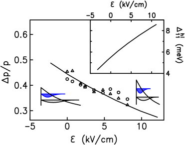
Figure 4: Spin splitting $\Delta p/p$ for a quasi-2D hole system in a (001) GaAs-Al_0.3Ga_0.7As single heterojunction at constant total density $p=1.84\times 10^{11}$ cm^-2, where the asymmetry was tuned by applying an electric field $\mathcal{E}_{\perp}$ perpendicular to the quasi-2D system hab04a . The inset shows the calculated HH-LH splitting $\Delta^{hl}_{11}$ that decreases as a function of $\mathcal{E}_{z}$.

V Multipole Expansion of the Spin Density Matrix

We can gain a more systematic understanding of the unusual spin-dependent phenomena in hole systems from the spin density matrix which is the fundamental object providing a complete description of the system. Neglecting the orbital degrees of freedom, spin-1/2 electron systems are characterized by a $2\times 2$ spin density matrix $\rho$, whereas in spin-3/2 hole systems $\rho$ becomes a $4\times 4$ matrix. The dominant character of the occupied eigenstates of hole systems depends on the quantization axis of the underlying $j=3/2$ basis functions. Obviously, observable quantities such as the spin polarization may not depend on this choice. Therefore, it is necessary to formulate the spin density matrix in a way such that observable quantities can be calculated independent of the particular choice for the basis functions that are used. Using the theory of invariants bir74 ; win03 it is possible to derive an invariant decomposition of the spin density matrix of $j=3/2$ hole systems that can be interpreted as a multipole expansion win04b . These multipoles indeed have the desired property that they can be evaluated and interpreted independent of the particular choice of basis functions.

Quite generally, neglecting small terms with cubic symmetry, the spin density matrix ${\rho}$ for systems with spin $j$ can be decomposed as follows win04b

$${\rho} = \sum_{\mathfrak{j}=0}^{2j}{{\bm{\mathrm{\rho}}}}_{\mathfrak{j}}\cdot{\bm{\mathrm{M}}}_{\mathfrak{j}}$$ (16a)

$$\equiv \rho_{0}\,M_{0}+{\bm{\mathcal{S}}}\cdot{\bm{\mathrm{M}}}_{1}+{\bm{\mathcal{Q}}}\cdot{\bm{\mathrm{M}}}_{2}+{\bm{\mathcal{O}}}\cdot{\bm{\mathrm{M}}}_{3}+\ldots.\hskip 20.00003pt$$ (16b)

The $2\mathfrak{j}+1$ quantities ${\bm{\mathrm{M}}}_{\mathfrak{j}}$, which we refer to as multipoles, are spherical tensors that transform according to the irreducible representations $\mathcal{D}_{\mathfrak{j}}$ of the point group SU(2). They are analogs of the vector of Pauli spin matrices familiar in electron systems. Each ${\bm{\mathrm{M}}}_{\mathfrak{j}}$ is a $(2\mathfrak{j}+1)$-dimensional vector with components $M_{\mathfrak{j}\mathfrak{m}}$, $-\mathfrak{j}\leq{\mathfrak{m}}\leq\mathfrak{j}$, which are $(2j+1)\times(2j+1)$ matrices. These matrices are orthonormal in the sense that $\operatorname{tr}(M^{\dagger}_{\mathfrak{j}\mathfrak{m}}\,M_{\mathfrak{j}^{\prime}\mathfrak{m}^{\prime}})=\delta_{\mathfrak{j}\mathfrak{j}^{\prime}}\delta_{\mathfrak{m}\mathfrak{m}^{\prime}}$. They can be calculated using standard angular momentum theory edm60 . $M_{\mathfrak{j}\mathfrak{m}}$ for spin-$1/2$ and spin-$3/2$ systems have been tabulated in Ref. win04b . The multipole moments ${{\bm{\mathrm{\rho}}}}_{\mathfrak{j}}$ give the weight of each multipole in the density matrix. Each ${{\bm{\mathrm{\rho}}}}_{\mathfrak{j}}$ is a $(2\mathfrak{j}+1)$-dimensional vector with scalar components $\rho_{\mathfrak{j}\mathfrak{m}}$. The components $\rho_{\mathfrak{j}\mathfrak{m}}$ of the moments ${\bm{\mathrm{\rho}}}_{\mathfrak{j}}$ can be obtained from

$$\rho^{\ast}_{\mathfrak{j}\mathfrak{m}}=\operatorname{tr}(M_{\mathfrak{j}\mathfrak{m}}\,\rho),$$ (17)

and the magnitude of each moment is given by

$$|\rho_{\mathfrak{j}}|^{2}=\sum_{\mathfrak{m}}(-1)^{\mathfrak{m}}\,\rho_{\mathfrak{j}\mathfrak{m}}\,\rho_{\mathfrak{j},-\mathfrak{m}}.$$ (18)

In Eq. (16) one can thus interpret the vectors ${\bm{\mathrm{M}}}_{\mathfrak{j}}$ as multipole operators that “measure” the moments ${\bm{\mathrm{\rho}}}_{\mathfrak{j}}$ of the system. For simplicity we assume that all orbital degrees of freedom are integrated over, so that ${\rho}$ depends only on the spin indices and does not depend on the wave vector ${\bm{\mathrm{k}}}$. Nevertheless, the coupling of spin and ${\bm{\mathrm{k}}}$ is present in the Hamiltonian through the spin-orbit interaction. We note that the dot product for spherical tensors appearing in Eq. (16) is defined in Ref. edm60 .

The moments ${{\bm{\mathrm{\rho}}}}_{\mathfrak{j}}$ provide a set of independent parameters characterizing the matrix ${\rho}$ win04b . The monopole $\rho_{0}$ is identified with the carrier density, while the dipole ${\bm{\mathrm{\rho}}}_{1}\equiv{\bm{\mathcal{S}}}$ corresponds to the spin polarization or Bloch vector at $B>0$. These are the only moments present in the density matrix of conduction electrons. In $j=3/2$ hole systems, a quadrupole ${\bm{\mathrm{\rho}}}_{2}\equiv{\bm{\mathcal{Q}}}$ is also present, which reflects the splitting between the HH and LH states discussed in the preceding sections. The octupole ${\bm{\mathrm{\rho}}}_{3}\equiv{\bm{\mathcal{O}}}$ is a unique feature of $j=3/2$ systems at $B>0$.

As discussed in Sec. II, the dynamics of $j=3/2$ hole systems is characterized by the $4\times 4$ Luttinger Hamiltonian $\mathcal{H}_{L}$. Obviously, the spherical tensor operators discussed here provide the most natural language to formulate the spherical approximation $\mathcal{H}_{s}$ of $\mathcal{H}_{L}$, i.e., instead of Eq. (4) we may write $\mathcal{H}_{s}$ analogous to Eq. (16) in the form lip70 ; suz74

$$\mathcal{H}_{s} = \sum_{\mathfrak{j}=0}^{3}\mathcal{H}_{\mathfrak{j}}=\sum_{\mathfrak{j}=0}^{3}a_{\mathfrak{j}}\,{\bm{\mathcal{K}}}_{\mathfrak{j}}\cdot{\bm{\mathcal{M}}}_{\mathfrak{j}}$$ (19b)

$$= -\frac{\hbar^{2}\,\gamma_{1}}{m_{0}}\,{\bm{\mathcal{K}}}_{0}\cdot{\bm{\mathrm{M}}}_{0}-2\sqrt{5}\,\kappa\mu_{\mathrm{B}}\,{\bm{\mathcal{K}}}_{1}\cdot{\bm{\mathrm{M}}}_{1}$$

$$+\sqrt{6}\,\frac{\hbar^{2}\,\bar{\gamma}}{m_{0}}\,{\bm{\mathcal{K}}}_{2}\cdot{\bm{\mathrm{M}}}_{2}+\zeta\,{\bm{\mathcal{K}}}_{3}\cdot{\bm{\mathrm{M}}}_{3}+\mathcal{H}_{\mathrm{c}}\>.\hskip 20.00003pt$$

The tensor operators ${\bm{\mathcal{K}}}_{\mathfrak{j}}$ (like the vectors ${\bm{\mathrm{M}}}_{\mathfrak{j}}$) are tabulated in Ref. win04b . The first term in Eq. (19b), which we interpret as a monopole, is equal to the first term in Eq. (4). The second term in Eq. (19b), which corresponds to a dipole, is the (spherically symmetric) Zeeman term (8). The third term in Eq. (19b), which corresponds to a quadrupole, is equal to the second term in (4). This term is responsible for the HH-LH splitting. The fourth term in Eq. (19b) corresponds to an octupole, which depends on ${\bm{\mathrm{k}}}$ and ${\bm{\mathrm{B}}}$. The prefactor $\zeta$ of this term is typically very small so that normally it can be neglected suz74 ; win04b . Obviously $\mathcal{H}_{1}=\mathcal{H}_{3}=0$ for zero magnetic field. We note that in Eq. (4) we considered only the terms with the lowest order of ${\bm{\mathrm{k}}}$ and ${\bm{\mathrm{B}}}$ so that we have $\mathcal{K}_{0}=k^{2}$ and ${\bm{\mathcal{K}}}_{1}={\bm{\mathrm{B}}}$. Higher-order terms as well as, e.g., strain-induced terms can be classified in the same way. For example, the most important strain-induced term is a quadrupole field (independent of ${\bm{\mathrm{k}}}$ win04b ). Finally, the cubic term $\mathcal{H}_{\mathrm{c}}$ reads

$$\begin{array}[b]{@{}r@{}l@{}}\mathcal{H}_{\mathrm{c}}=\displaystyle-\frac{\hbar^{2}}{2m_{0}}&\,\sqrt{6}\,(\gamma_{3}-\gamma_{2})\,\Bigl{\{}\left[{\bm{\mathcal{K}}}_{2}\times{\bm{\mathrm{M}}}_{2}\right]_{4,-4}\\[8.61108pt] &+{\textstyle\frac{\sqrt{70}}{5}}\left[{\bm{\mathcal{K}}}_{2}\times{\bm{\mathrm{M}}}_{2}\right]_{4,0}+\left[{\bm{\mathcal{K}}}_{2}\times{\bm{\mathrm{M}}}_{2}\right]_{4,4}\Bigr{\}},\end{array}$$ (20)

where the product of spherical tensors is defined in Ref. edm60 . Our prefactor of $\mathcal{H}_{\mathrm{c}}$ differs slightly from the one given in Ref. lip70 due to the different normalization of the tensor operators ${\bm{\mathcal{K}}}_{2}$ and ${\bm{\mathrm{M}}}_{2}$ adopted from Ref. win04b .

VI Multipole Moments Induced by a Magnetic Field

To gain a qualitative understanding of the relevance of the spin multipoles ${\bm{\mathrm{\rho}}}_{\mathfrak{j}}$, it is helpful to study the response of a 2D hole systems to an external magnetic field $B$. For zero magnetic field, the system is characterized by a large quadrupole moment close to its maximum value. This result reflects the fact that the HH-LH splitting is the most important effect in a 2D HH system and the multipole expansion (16) is the natural language to describe this effect. A perpendicular magnetic field results in a large dipole moment (i.e., a large spin polarization), as expected from Fig. 1. Of course, for a perpendicular magnetic field we also need to take into account the formation of Landau levels. A low-density 2D electron system can become fully spin-polarized without forming Landau levels when an in-plane magnetic field is applied oka99 ; tut03 . When the Zeeman energy becomes larger then the ($B$ dependent) Fermi energy, the minority spin subband is completely depopulated and the system becomes fully spin-polarized. In 2D HH systems, on the other hand, the spin polarization is generally suppressed when an in-plane magnetic field is applied win04a ; win04b . As an example, Fig. 5 shows the calculated response of a 2D HH system in a symmetric (100) GaAs-Al_0.3Ga_0.7As quantum well with hole density $p=5\times 10^{10}$ cm^-2 and well width $w=150$ Å.

Figure 5: (a) Spin subband density $p_{-}$ of the HH minority spin subband and (b-d) normalized multipole moments $\tilde{\rho}_{i}$ as a function of the in-plane magnetic field $B_{\|}$ calculated self-consistently for a symmetric (100) GaAs-Al_0.3Ga_0.7As quantum well with hole density $p=5\times 10^{10}$ cm^-2 and well width $w=150$ Å. Adapted from Ref. win04b .

We can see in Fig. 5 that the complete depopulation of the HH minority spin subband due to $B_{\|}$ does not imply full spin polarization of the system win04a ; win04b . In Fig. 5, the minority spin subband is completely depopulated at $B_{D}\approx 23.9$ T while $\tilde{\mathcal{S}}(B_{D})\approx 0.144$. Here we use the tilde to indicate that we have normalized $\rho_{1}=\mathcal{S}$ with respect to the total 2D density $2\rho_{0}$. We see that the spin polarization $\tilde{\mathcal{S}}(B_{\|})$ is always much smaller than $3/2\sqrt{5}\approx 0.67$, the value of $\tilde{\mathcal{S}}$ in a fully spin-polarized HH system and it is unrelated with the depopulation of the minority spin subband [Fig. 5(a)]. Most surprisingly we even have a sign reversal of the spin polarization vector at $B_{\|}\approx 18.4$ T which is a unique feature of 2D HH systems win04a . The derivative of $\tilde{\mathcal{S}}(B_{\|})$ is discontinuous at $B_{\|}=B_{D}$. At $B_{\|}=0$ the quadrupole moment $\tilde{\mathcal{Q}}$ is slightly smaller than $1/2$, the value of $\tilde{\mathcal{Q}}$ in a pure HH system. This is a consequence of the ${\bm{\mathrm{k}}}_{\|}$-induced HH-LH mixing which was fully taken into account in Fig. 5. For $B_{\|}>0$ we observe only a small decrease of $\tilde{\mathcal{Q}}$. This is due to the fact that the HH-LH splitting $E^{h}_{1}-E^{l}_{1}\approx 6.7$ meV [i.e., the denominator in Eq. (9)] is the largest energy scale in the system so that the HH states have a frozen angular momentum perpendicular to the 2D plane, as illustrated in Fig. 1. For comparison, we note that the Zeeman energy splitting of the HH subband at $B_{D}$ is $\sim 0.4$ meV.

It is remarkable that the octupole moment $\tilde{\mathcal{O}}$ at $B_{\|}=B_{D}$ is close to $1/\sqrt{2}\approx 0.71$, the largest possible value of $\tilde{\rho}_{3}$ in a 2D HH system. This value is essentially independent of whether we use the Luttinger Hamiltonian (19) without or with the octupole term proportional to $\zeta$. This result reflects the fact that, unlike the simpler case of spin-1/2 electron systems, we cannot establish a simple one-to-one correspondence between the multipoles in the Hamiltonian (19) and the multipoles of the same degree in the spin density matrix (16). On the other hand, these findings suggest that an in-plane magnetic field $B_{\|}$ provides an efficient tool to study 2D HH systems with a large octupole moment but with a small dipole moment (i.e., with a small spin polarization). Note that we can use an in-plane magnetic field to obtain a significant out-of-plane spin polarization using the anisotropic Zeeman splitting (the component $g_{xz}^{\ast}$ of the $g$ factor) on low-symmetry surfaces such as the (113) surface, see Fig. 2 (Ref. win05 ).

VII Spin Precession of Holes

VII.1 General Analysis

Before discussing hole spin precession, we will review briefly Larmor precession in electron systems lanIV1e . It is well known that the dipole moment (spin polarization) of a spin-$1/2$ system performs a precessing motion in an external magnetic field ${\bm{\mathrm{B}}}$. It can be derived via the Heisenberg equation of motion (HEM) for the spin operator ${\bm{\mathrm{M}}}_{1}={\bm{\mathrm{\sigma}}}$ propagating due to a Zeeman term $\mathcal{H}_{1}\equiv\frac{1}{2}g^{\ast}\mu_{\mathrm{B}}\;{\bm{\mathrm{\sigma}}}\cdot{\bm{\mathrm{B}}}$,

$$\frac{d{\bm{\mathrm{\sigma}}}}{dt}=\frac{1}{i\hbar}\;[{\bm{\mathrm{\sigma}}},\mathcal{H}_{1}]=g^{\ast}\mu_{\mathrm{B}}\;{\bm{\mathrm{\sigma}}}\times{\bm{\mathrm{B}}}\,,$$ (21)

where ${\bm{\mathrm{\sigma}}}$ at time $t=0$ is the vector of Pauli spin matrices. If the only spin-dependent term of the full Hamiltonian is $\mathcal{H}_{1}$, the HEM (21) is valid also for particles with $j>1/2$ (with ${\bm{\mathrm{\sigma}}}$ replaced by the appropriate angular momentum matrices for $j>1/2$). Taking the expectation value of Eq. (21) with respect to a state $|\psi\rangle$ yields $\langle\dot{{\bm{\mathrm{\sigma}}}}\rangle=g^{\ast}\mu_{\mathrm{B}}\;\langle{\bm{\mathrm{\sigma}}}\rangle\times{\bm{\mathrm{B}}}$, which can be interpreted as Ehrenfest’s theorem sak94 applied to a spin-$j$ system.

In the context of conventional spin precession lanIV1e it appears natural that the right-hand side of Eq. (21) can be expressed as a linear combination of spin operators $\sigma_{\mathfrak{m}}$. This implies that the HEM for the components $\sigma_{\mathfrak{m}}$ of ${\bm{\mathrm{\sigma}}}$ are closed. Using the language of multipole moments, we see here that for spin-$1/2$ systems the HEM of the dipole ${\bm{\mathrm{M}}}_{1}={\bm{\mathrm{\sigma}}}$ is decoupled from the HEM of the monopole $M_{0}$. Obviously, the HEM for $M_{0}$ is trivial, $\dot{M}_{0}=0$, which reflects the conservation of the probability density. We also note that Eq. (21) preserves the length of the Bloch vector $\langle{\bm{\mathrm{\sigma}}}\rangle$, i.e., $d|\langle{\bm{\mathrm{\sigma}}}\rangle|/dt=0$. This is equivalent to the statement that the magnitude of the dipole moment ${\bm{\mathrm{\rho}}}_{1}={\bm{\mathcal{S}}}$ does not depend on time, $\mathcal{S}(t)=\mathrm{constant}$, which reflects the conservation of energy in the system. (Here we ignore scattering and spin relaxation cul07 .)

We proceed to study the corresponding equations of motion of the multipoles ${\bm{\mathrm{M}}}_{\mathfrak{j}}$ of spin-$3/2$ systems. While the dipole term in the multipole expansion of the Hamiltonian can always be interpreted as a Zeeman-like term with an external or effective magnetic field, no such interpretation is possible for the higher multipoles in Eq. (19) including the quadrupole term. Therefore, the simple picture of a spin precessing around an effective Zeeman field is not applicable to holes. Nevertheless, the spin dynamics of hole systems can be viewed as a precession, if precession is understood as a nontrivial periodic motion in spin space described by an equation of the type $\frac{d\mathcal{S}}{dt}=\frac{i}{\hbar}[\mathcal{H},\mathcal{S}]$ for a suitably generalized spin operator $\mathcal{S}$ and spin Hamiltonian $\mathcal{H}$. However, the HEM for the different ${\bm{\mathrm{M}}}_{\mathfrak{j}}$ cannot be decoupled which has important consequences for the spin precession of hole systems cul06 .

Equation (19b) suggests that we study first the HEM

$$\frac{d{\bm{\mathrm{M}}}_{\mathfrak{j}}}{dt}=\frac{1}{i\hbar}\;[{\bm{\mathrm{M}}}_{\mathfrak{j}},\mathcal{H}_{\mathfrak{j}^{\prime}}]\,.$$ (22)

Making use of Eq. (19b), this equation can be decomposed into

$$\frac{d{\bm{\mathrm{M}}}_{\mathfrak{j}}}{dt}=\frac{a_{\mathfrak{j}^{\prime}}}{i\hbar}\,[{\bm{\mathrm{M}}}_{\mathfrak{j}},{\bm{\mathrm{M}}}_{\mathfrak{j}^{\prime}}]\cdot{\bm{\mathcal{K}}}_{\mathfrak{j}^{\prime}},$$ (23)

where the dot product is between ${\bm{\mathrm{M}}}_{\mathfrak{j}^{\prime}}$ and ${\bm{\mathcal{K}}}_{\mathfrak{j}^{\prime}}$. The commutator is an antisymmetric tensor product that may be further decomposed into multipoles using standard angular momentum algebra edm60 :

$$[M_{\mathfrak{j}\mathfrak{m}},M_{\mathfrak{j}^{\prime}\mathfrak{m}^{\prime}}]=\sum_{\mathfrak{J},\mathfrak{M}}C_{\mathfrak{j}\mathfrak{m}\,\mathfrak{j}^{\prime}\mathfrak{m}^{\prime}}^{\mathfrak{J}\mathfrak{M}}\left[1-(-1)^{(\mathfrak{j}+\mathfrak{j}^{\prime}+J)}\right]M_{\mathfrak{J}\mathfrak{M}}.$$ (24)

Here, the $C_{\mathfrak{j}\mathfrak{m}\,\mathfrak{j}^{\prime}\mathfrak{m}^{\prime}}^{\mathfrak{J}\mathfrak{M}}$ are Clebsch-Gordan coefficients for which the phase convention of Ref. edm60 has been adopted. Angular momentum conservation constrains the sum to $|\mathfrak{j}-\mathfrak{j}^{\prime}|\leq{\mathfrak{J}}\leq\mathfrak{j}+\mathfrak{j}^{\prime}$ and $-{\mathfrak{J}}\leq{\mathfrak{M}}\leq{\mathfrak{J}}$. The multipole components $M_{\mathfrak{J}\mathfrak{M}}$, which appear on the RHS of Eq. (24), are those satisfying the condition $\mathfrak{j}+\mathfrak{j}^{\prime}+{\mathfrak{J}}=\mathrm{odd}$. The invariant decomposition of the RHS of Eq. (22) is summarized in Table 1 asymprod . As discussed above, a dipole ${\bm{\mathrm{M}}}_{1}$ evolving under the action of $\mathcal{H}_{1}$ describes the well-known Larmor precession of holes lanIV1e . Table 1 shows, as expected, that in this case the RHS of Eq. (22) yields only ${\bm{\mathrm{M}}}_{1}$, i.e., the HEM for a dipole, which couples to a magnetic field through a Zeeman term, is closed. However, the most remarkable entry in the table is the one for ${\bm{\mathrm{M}}}_{2}$ propagating in time due to a quadrupole $\mathcal{H}_{2}$, the spin-orbit interaction that gives rise to the HH–LH coupling. We see here that the HEM for the components of ${\bm{\mathrm{M}}}_{2}$ are not closed. A quadrupole ${\bm{\mathrm{M}}}_{2}$ precessing in a quadrupole field “decays” into a dipole ${\bm{\mathrm{M}}}_{1}$ and an octupole ${\bm{\mathrm{M}}}_{3}$. This implies that spin precession of an initially unpolarized system can give rise to spin polarization, even though $B=0$. [As mentioned above, we use the term spin precession for any HEM (22) with $\mathfrak{j},\mathfrak{j}^{\prime}>0$.]

Table 1: Irreducible representations $\mathcal{D}_{\mathfrak{j}}$ of $SU(2)$ of the (linear combinations of) multipole ${\bm{\mathrm{M}}}_{\mathfrak{j}}$ contained in an invariant decomposition of $(1/i\hbar)\;[{\bm{\mathrm{M}}}_{\mathfrak{j}},\mathcal{H}_{\mathfrak{j}^{\prime}}]$.

$\begin{array}[]{c@{\hspace{2em}}cccc}\hline\cr\hline\cr\hfil\hskip 20.00003pt&\mathcal{H}_{0}&\mathcal{H}_{1}&\mathcal{H}_{2}&\mathcal{H}_{3}\\ \hline\cr M_{0}\hfil\hskip 20.00003pt&0&0&0&0\\ {\bm{\mathrm{M}}}_{1}\hfil\hskip 20.00003pt&0&\mathcal{D}_{1}&\mathcal{D}_{2}&\mathcal{D}_{3}\\ {\bm{\mathrm{M}}}_{2}\hfil\hskip 20.00003pt&0&\mathcal{D}_{2}&\mathcal{D}_{1}\oplus\mathcal{D}_{3}&\mathcal{D}_{2}\\ {\bm{\mathrm{M}}}_{3}\hfil\hskip 20.00003pt&0&\mathcal{D}_{3}&\mathcal{D}_{2}&\mathcal{D}_{1}\oplus\mathcal{D}_{3}\\ \hline\cr\hline\cr\end{array}$

We want to determine and interpret the explicit time evolution of $\rho$. This calculation is most easily carried out in the Schrödinger picture, which reflects the equivalence of the Heisenberg and Schrödinger pictures for this problem. Our final results below are independent of representation. In the absence of external fields and disorder, the density matrix satisfies the quantum Liouville equation

$$\frac{\partial\rho}{\partial t}=\frac{i}{\hbar}\,[\rho,\mathcal{H}].$$ (25)

Note the sign difference between the Liouville and Heisenberg equations. The formal solution is $\rho(t)=e^{-i\mathcal{H}t/\hbar}\rho(0)e^{i\mathcal{H}t/\hbar}$, where $e^{i\mathcal{H}t/\hbar}$ is the time evolution operator (which can often be evaluated in closed form).

VII.2 Precession of a Single Spin

We consider first an example where we assume the hole spin to be oriented initially along the $z$-direction, $m_{j}=+3/2$, so that

$$\tilde{\rho}(t=0)=\frac{1}{2}M_{0,0}+\frac{3}{2\sqrt{5}}M_{1,0}+\frac{1}{2}M_{2,0}+\frac{1}{2\sqrt{5}}M_{3,0},$$ (26)

where the tilde indicates that $\rho$ has been normalized with respect to the total density $2\rho_{0}$. This equation demonstrates that, in general, the density matrix of holes cannot be written simply as the sum of a monopole and a dipole. The higher multipoles will be present, too win05 .

We want to restrict ourselves to $\mathcal{H}=\mathcal{H}_{0}+\mathcal{H}_{2}$, i.e., $B=0$. Table 1 shows that $\rho$ evolves as a combination of a dipole, a quadrupole, and an octupole. The implications of this fact are best seen by following the motion of the Bloch vector ${\bm{\mathrm{S}}}(t)=\sqrt{5}\,\tilde{{\bm{\mathcal{S}}}}(t)$

$$\begin{array}[b]{rl}{\bm{\mathrm{S}}}(t)={\textstyle\frac{3}{2}}\big{\{}&\hat{{\bm{\mathrm{S}}}}_{0}\left[\cos^{2}(\omega t)+c^{4}\sin^{2}(\omega t)\right]\\[4.30554pt] &\displaystyle{}+\hat{{\bm{\mathrm{\kappa}}}}\,s\,c\,(1+c^{2})\,\sin^{2}(\omega t)\\[5.16663pt] &\displaystyle{}+(\hat{{\bm{\mathrm{S}}}}_{0}\times\hat{{\bm{\mathrm{\kappa}}}})\,2\,s\,c\,\sin(\omega t)\cos(\omega t)\big{\}},\end{array}$$ (27)

where the hat denotes unit vectors; we have ${\bm{\mathrm{S}}}_{0}={\bm{\mathrm{S}}}(t=0)$; $c=\hat{{\bm{\mathrm{S}}}}_{0}\cdot\hat{{\bm{\mathrm{k}}}}$ is the cosine of the angle between $\hat{{\bm{\mathrm{S}}}}_{0}$ and ${\bm{\mathrm{k}}}$; $s$ is the sine of the same angle; and ${\bm{\mathrm{\kappa}}}={\bm{\mathrm{k}}}-(\hat{{\bm{\mathrm{S}}}}_{0}\cdot{\bm{\mathrm{k}}})\hat{{\bm{\mathrm{S}}}}_{0}$ is the vector orthogonal to ${\bm{\mathrm{S}}}_{0}$ in the $({\bm{\mathrm{S}}}_{0},{\bm{\mathrm{k}}})$ plane. We see that the trajectory ${\bm{\mathrm{S}}}(t)$ in spin space is independent of the Luttinger parameters; only the frequency $\omega=(E_{h}-E_{l})/2\hbar\simeq\bar{\gamma}\hbar k^{2}/m_{0}$ depends on $\bar{\gamma}$ and $k$. When ${\bm{\mathrm{S}}}_{0}$ is parallel to ${\bm{\mathrm{k}}}$ (i.e., $c=1$), we get ${\bm{\mathrm{S}}}(t)={\bm{\mathrm{S}}}_{0}$, which is due to the fact that the initial state is an eigenstate of the Hamiltonian. In general, neither the magnitude nor the orientation of the Bloch vector are conserved. This is illustrated in Fig. 6 showing ${\bm{\mathrm{S}}}(t)$ for an angle of $60^{\circ}$ between $\hat{{\bm{\mathrm{S}}}}_{0}$ and ${\bm{\mathrm{k}}}$. Helicity ${\bm{\mathrm{S}}}\cdot{{\bm{\mathrm{k}}}}$ is conserved, a well-known fact about this model, which sheds additional light on spin precession in hole systems. Since $\frac{d}{dt}({\bm{\mathrm{S}}}\cdot{{\bm{\mathrm{k}}}})=0$ and the wave vector is not changing, $\frac{d{\bm{\mathrm{S}}}}{dt}\cdot{{\bm{\mathrm{k}}}}=0$. Therefore, whenever the magnitude of the spin changes, the angle between spin and wave vector must change in order to preserve the projection of ${\bm{\mathrm{S}}}$ onto ${{\bm{\mathrm{k}}}}$. As a consequence, no nontrivial spin precession occurs when ${\bm{\mathrm{S}}}\perp{\bm{\mathrm{k}}}$ (or ${\bm{\mathrm{S}}}\parallel{\bm{\mathrm{k}}}$). We note that energy is also conserved for spin precession in hole systems. Yet for $B>0$, when $\mathcal{H}=\mathcal{H}_{0}+\mathcal{H}_{1}+\mathcal{H}_{2}$, it can be shown that, in the general case, energy is transferred back and forth between $\mathcal{H}_{1}$ and $\mathcal{H}_{2}$ as time progresses. For an LH spin ($m_{j}=+1/2$) we obtain similar to Eq. (27)

$$\begin{array}[b]{rl}{\bm{\mathrm{S}}}(t)=&\hat{{\bm{\mathrm{S}}}}_{0}\left[{\textstyle\frac{1}{2}}\,+{\textstyle\frac{3}{2}}\,s^{2}(2-3s^{2})\,\sin^{2}(\omega t)\right]\\[4.30554pt] &\displaystyle{}+{\textstyle\frac{3}{2}}\,\hat{{\bm{\mathrm{\kappa}}}}\,s\,c\,(1-3c^{2})\,\sin^{2}(\omega t)\\[5.16663pt] &\displaystyle{}-3\,(\hat{{\bm{\mathrm{S}}}}_{0}\times\hat{{\bm{\mathrm{\kappa}}}})\,s\,c\,\sin(\omega t)\cos(\omega t).\end{array}$$ (28)

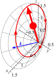
Figure 6: Precession of the Bloch vector ${\bm{\mathrm{S}}}$ (bold arrow) about the wave vector ${\bm{\mathrm{k}}}$ when the angle between the two is initially $60^{\circ}$. We have assumed ${\bm{\mathrm{S}}}(t=0)$ is parallel to the $z$ axis, and ${\bm{\mathrm{k}}}$ lies in the $xz$ plane. Taken from Ref. cul06 .

The analysis above highlights a major advantage of our method. Although most of the results presented here can be derived also using wave functions, the decomposition of $\rho$ and $\mathcal{H}$ into multipoles makes the symmetry of the problem transparent lip70 . In particular, the interdependence of the multipoles would not be evident if one used wave functions. Moreover, the multipoles do not rely on a particular choice of basis functions win04b — in that sense the multipoles are gauge-invariant.

VII.3 Holes Turning a Corner at $B=0$: Alternating Spin Polarization

We would like to relate our work to recent experiments by Grayson et al. gra04 ; gra05 which demonstrated that a high-quality bent heterostructure can be grown on top of a pre-cleaved corner substrate that allows one to drive the charge carriers around an atomically sharp $90^{\circ}$ corner. Grayson’s experiments were performed on a 2D electron system in a GaAs/AlGaAs quantum well. We show here that a similar system containing holes gives rise to fascinating new physics cul06 . The setup is sketched in Fig. 7(a). We assume $B=0$ so that the Hamiltonian is $\mathcal{H}=\mathcal{H}_{0}+\mathcal{H}_{2}$. An unpolarized HH wave packet travels in the 2D channel L₁ in the $+x$ direction. For simplicity we assume that all orbital degrees of freedom are integrated over, so that ${\rho}$ depends only on the spin indices and does not depend on the wave vector ${\bm{\mathrm{k}}}$. Nevertheless, the coupling of spin and ${\bm{\mathrm{k}}}$ is present in the Hamiltonian through the spin-orbit interaction. The magnitudes of the normalized moments at $t\leq 0$ (i.e., before reaching the corner) are $\tilde{\mathcal{S}}=\tilde{\mathcal{O}}=0$ and $\tilde{\mathcal{Q}}=1/2$. The spin quantization axis of the HH states in L₁ is parallel to the $z$-direction. After the wave packet has passed the corner, the HH states are not eigenstates of $\mathcal{H}_{2}$, their spin quantization axis being perpendicular to the spin quantization axis supported by the quadrupole field in L₂. Therefore, the quadrupole and octupole moments in L₂ oscillate in time

$$|\tilde{{\bm{\mathcal{Q}}}}(t)|^{2} = (1/16)+(3/16)\cos^{2}(\omega_{z}t)$$ (29a)

$$|\tilde{{\bm{\mathcal{O}}}}(t)|^{2} = (3/16)\sin^{2}(\omega_{z}t),$$ (29b)

with precession frequency $\omega_{z}=(E_{h}-E_{l})/2\hbar\simeq 2\bar{\gamma}\hbar\pi^{2}/m_{0}w^{2}$. This frequency can be tailored by varying the width $w$ of the 2D channel. For GaAs in the spherical approximation we have $\bar{\gamma}=2.58$ and we take $w=10$ nm, yielding a precession period $2\pi/\omega_{z}\approx 11$ ps.

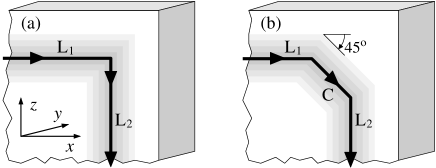
Figure 7: A bent structure allows holes to be driven around a corner gra04 ; gra05 . (a) An idealized representation of the corner device. (b) A more realistic model of the corner, as discussed in the text. In regions C and L₂ the spin polarization oscillates as a function of time. Taken from Ref. cul06 .

For the simplified geometry of Fig. 7(a) the spin polarization $\tilde{\mathcal{S}}$ in L₂ remains zero, as required by the conservation of helicity discussed above. However, assuming a sharp $90^{\circ}$ corner for an ideal 2D system is certainly an oversimplification, even when the corresponding quasi 2D system has atomically sharp interfaces gra04 . A more realistic treatment can be obtained by modeling the transition region between the channels L₁ and L₂ as a sequence of two $45^{\circ}$ corners as sketched in Fig. 7(b). Once again, an unpolarized HH wave packet travels in channel L₁ in the $+x$ direction, the initial conditions being the same as in the previous example. If the HH wave packet enters the central region C at $t=0$, we obtain for the squared normalized moments in this region

$$|\tilde{{\bm{\mathcal{S}}}}(t)|^{2} = (9/80)\;\sin^{2}(\omega_{z}t)$$ (30a)

$$|\tilde{{\bm{\mathcal{Q}}}}(t)|^{2} = 1/64+(15/64)\cos^{2}(\omega_{z}t)$$ (30b)

$$|\tilde{{\bm{\mathcal{O}}}}(t)|^{2} = (39/320)\;\sin^{2}(\omega_{z}t).$$ (30c)

Equation (30a) shows that the initially unpolarized hole current acquires an alternating spin polarization $\tilde{{\bm{\mathcal{S}}}}(t)$ due to spin precession at $B=0$. In Cartesian coordinates, the Bloch vector in region C reads $\tilde{{\bm{\mathrm{S}}}}(t)=[0,-\frac{3}{4\sqrt{5}}\,\sin(\omega_{z}t),0]$. When the HH wave packet enters the channel L₂ it continues to precess. We get for the spin polarization

$$\tilde{\mathcal{S}_{y}}=\frac{-3}{8\sqrt{5}}\left[\cos^{2}\left(\frac{\omega_{z}T}{2}\right)\sin(\omega_{z}t)+2\sin(\omega_{z}T)\sin^{2}\left(\frac{\omega_{z}t}{2}\right)\right].$$ (31)

Here $T$ is the time required to traverse C which depends on the length of C and the magnitude of the in-plane wave vector. It determines the fraction of the spin polarization in L₂ that will be oscillating. If we take the length of C to be of the order of the channel width, namely $w=10$ nm, and the initial wave vector $k_{F}=0.1$ nm^-1, we get $T\sim 0.5$ ps. The amplitude of $\tilde{\mathcal{S}_{y}}$ in this case is approximately 0.1. We omit here the qualitatively similar but more complicated expressions for $\tilde{{\bm{\mathcal{Q}}}}(t)$ and $\tilde{{\bm{\mathcal{O}}}}(t)$. We note also that the approach in Fig. 7(b) can be further extended in a transfer-matrix-like approach in order to describe more complicated geometries.

VIII Spin Relaxation in Hole Systems

Spin relaxation in spin-1/2 electron systems has received considerable attention dya72 ; dya86 ; pik84 ; dya71 ; dya06 ; kis00 ; son02 ; hua03 ; ohn99 ; sli90 ; dzh04 ; ave99 ; ave02 ; ave06 ; gri02 ; ell54 ; yaf63 ; qi03 ; mis04 ; lau01 ; kai04 ; bro04 ; ble04 ; ohn07 . For electrons the spin-orbit interaction can always be represented by a Zeeman-like term (13) with an effective wave vector-dependent magnetic field ${\bm{\mathcal{B}}}({\bm{\mathrm{k}}})\equiv\hbar\,{\bm{\mathrm{\Omega}}}({\bm{\mathrm{k}}})$. The electron spin precesses about this field with frequency $\Omega=|{\bm{\mathrm{\Omega}}}({\bm{\mathrm{k}}})|$. An important parameter is the product of the frequency $\Omega$ times the momentum relaxation time $\tau_{p}$. In the ballistic (clean) regime no scattering occurs, so that $\Omega\tau_{p}\rightarrow\infty$. The weak scattering regime is characterized by fast spin precession and little momentum scattering, yielding $\Omega\,\tau_{p}\gg 1$. In the strong momentum scattering regime $\Omega\,\tau_{p}\ll 1$. Electron systems are often in the strong scattering regime and most past work has concentrated on this case.

As discussed in Sec. V, for spin-3/2 holes the spin-orbit interaction cannot be written as an effective field, and spin precession is qualitatively different (Sec. VII). Since spin-orbit coupling is more important in the valence band, hole spin information is lost faster, and the relative strengths of spin-orbit coupling and momentum scattering can vary. Yet spin relaxation of spin-3/2 holes has also been studied to a lesser extent, both experimentally hil02 and theoretically ave02 ; dya84a ; ser05 ; lue06 ; uen90 ; fer91 .

Recently we were able to derive a general unifying quantitative theory for the return to equilibrium of excess spin polarizations in the conduction and valence bands of semiconductors brought about by the interplay of spin precession and momentum scattering cul07 . Spin polarization decay in different regimes of momentum scattering in spin-1/2 electron and spin-3/2 hole systems contains considerable rich and novel physics. For example, spin polarization decay has often been assumed to be proportional to $e^{-t/\tau_{s}}$, where $\tau_{s}$ is referred to as the spin relaxation time. However, if the magnitude of the spin-orbit interaction is anisotropic (as is usually the case in systems studied experimentally), spin-polarization decay can occur even in the absence of momentum scattering. This process is characterized by a non-exponential decay and is sensitive to the initial conditions, and cannot therefore be described by a spin relaxation time. Weak momentum scattering introduces a spin relaxation time $\tau_{s}\propto\tau_{p}$ (unlike strong momentum scattering, which gives the well-known dya72 ; pik84 trend $\tau_{s}\propto\tau_{p}^{-1}$), yet even in the presence of weak momentum scattering a fraction of the polarization may survive at long times. Indeed, in the ballistic and weak momentum scattering regimes, the concept of a spin relaxation time is of very limited applicability and in general does not provide an accurate description of the physics of spin polarization decay.

VIII.1 Time Evolution of the Density Matrix

We assume a nonequilibrium spin polarization has been generated in a homogeneous, unstructured system and study its time evolution in the absence of external fields. The system is described by a density matrix, which in principle has matrix elements diagonal and off-diagonal in momentum space. Since the spin operator is diagonal in the wave vector ${\bm{\mathrm{k}}}$, we will only be concerned with the part of the density matrix diagonal in momentum space, which is denoted by $\rho_{\bm{\mathrm{k}}}$.

The spin density is given by $\langle{\bm{\mathrm{S}}}\rangle\equiv\operatorname{tr}({\bm{\mathrm{S}}}\rho_{\bm{\mathrm{k}}})=\operatorname{tr}({\bm{\mathrm{S}}}\bar{\rho}_{k})$, where ${\bm{\mathrm{S}}}$ is the spin operator, the trace includes ${\bm{\mathrm{k}}}$ and spin, and the overline represents averaging over directions in momentum space. Only the isotropic part $\bar{\rho}_{k}$ of the density matrix is responsible for spin population decay pik84 . It is therefore convenient to divide $\rho_{\bm{\mathrm{k}}}$ into $\rho_{\bm{\mathrm{k}}}=\bar{\rho}_{k}+g_{\bm{\mathrm{k}}}$, where $g_{\bm{\mathrm{k}}}$ is the anisotropic part of $\rho_{\bm{\mathrm{k}}}$. Based on the quantum Liouville equation, we obtain an equation describing the time evolution of $\rho_{\bm{\mathrm{k}}}$ (Ref. ave02 ), which in turn is split into a set of equations for $\bar{\rho}_{k}$ and $g_{\bm{\mathrm{k}}}$ similar to those found by Pikus and Titkov pik84 :

$$\frac{\partial\bar{\rho}_{k}}{\partial t}+\frac{i}{\hbar}\,\overline{[\mathcal{H},g_{\bm{\mathrm{k}}}]} = 0,$$ (32a)

$$\frac{\partial g_{\bm{\mathrm{k}}}}{\partial t}+\frac{i}{\hbar}\,[\mathcal{H},g_{\bm{\mathrm{k}}}]+\frac{g_{\bm{\mathrm{k}}}}{\tau_{p}} = -\frac{\partial\bar{\rho}_{k}}{\partial t}-\frac{i}{\hbar}\,[\mathcal{H},\bar{\rho}_{k}].\hskip 20.00003pt$$ (32b)

Here, $\mathcal{H}$ is, in general, the full Hamiltonian; yet the spin-diagonal part of $\mathcal{H}$ commutes with $\rho_{\bm{\mathrm{k}}}$ so that it is not relevant for spin relaxation. We assume elastic, spin-independent scattering, implying that the collision term involving $\bar{\rho}_{k}$ vanishes pik84 . For isotropic ($s$ wave) scattering due to, e.g., screened impurities the remainder is proportional to the inverse of the scalar momentum relaxation time $1/\tau_{p}$ (Ref. multi_tau ). A solution to Eq. (32b) can be obtained by making the transformation $g_{\bm{\mathrm{k}}}=e^{-i\mathcal{H}t/\hbar}g_{{\bm{\mathrm{k}}}}^{H}\,e^{i\mathcal{H}t/\hbar}$, which is analogous to the customary switch to the Heisenberg picture. Substituting this solution into Eq. (32a) yields cul07

$$\begin{array}[b]{rl}\displaystyle\frac{\partial\bar{\rho}_{k}}{\partial t}+\frac{i}{\hbar\tau_{p}}\int_{0}^{t}\!dt^{\prime}&\displaystyle e^{-(t-t^{\prime})/\tau_{p}}\,\overline{e^{-i\mathcal{H}(t-t^{\prime})/\hbar}\,[\mathcal{H},\bar{\rho}_{k}(t^{\prime})]\,e^{i\mathcal{H}(t-t^{\prime})/\hbar}}\\[9.47217pt] &\displaystyle=-\frac{i}{\hbar}\,e^{-t/\tau_{p}}\,\overline{e^{-i\mathcal{H}t/\hbar}\,[\mathcal{H},\rho_{{\bm{\mathrm{k}}}0}]\,e^{i\mathcal{H}t/\hbar}},\end{array}$$ (33)

where $\rho_{{\bm{\mathrm{k}}}0}$ is the initial value $\rho_{\bm{\mathrm{k}}}(t=0)$. This equation describes the precession-induced decay of spin polarization in all regimes of momentum scattering for both spin-1/2 electrons and spin-3/2 holes in semiconductors. It does not anticipate any particular form of spin polarization decay, such as exponential decay.

The form of the initial density matrix $\rho_{{\bm{\mathrm{k}}}0}$ is important and lies at the root of the physics discussed in the remainder of this section. In general $\rho_{{\bm{\mathrm{k}}}0}$ has two contributions, $\rho_{{\bm{\mathrm{k}}}0}=\rho_{{\bm{\mathrm{k}}}0}^{\|}+\rho_{{\bm{\mathrm{k}}}0}^{\perp}$. The component $\rho_{{\bm{\mathrm{k}}}0}^{\|}$ commutes with $\mathcal{H}$ and $\rho_{{\bm{\mathrm{k}}}0}^{\perp}$ is simply the remainder. $\rho_{{\bm{\mathrm{k}}}0}^{\|}$ is a matrix that is parallel to the Hamiltonian, and represents the fraction of the initial spin polarization that does not precess, or alternatively the fraction of the initial spins that are in eigenstates of the Hamiltonian. $\rho_{{\bm{\mathrm{k}}}0}^{\perp}$ is orthogonal to the Hamiltonian, and represents the fraction of the initial spin polarization that does precess.

VIII.2 Regimes of Spin Polarization Decay in Spin-3/2 Hole Systems

In general, Eq. (33) allows one to distinguish and describe several different regimes of spin polarization decay by comparing the precession frequency $\Omega({\bm{\mathrm{k}}})$ with the momentum relaxation time $\tau_{p}$ cul07 . In the following we consider spin-3/2 holes described by the Luttinger Hamiltonian (1). We work first in the spherical approximation, Eq. (19).

VIII.2.1 Exponential Decay in the Strong Momentum Scattering Regime

A solution to Eq. (33) characterizing relaxation is understood as exponential decay of the form

$$\bar{\rho}_{k}(t)=e^{-\Gamma_{s}t}\,\bar{\rho}_{k0},$$ (34)

where $\Gamma_{s}$ is generally a second-rank tensor that represents the inverse of the spin relaxation time $\tau_{s}$. Such a simple solution of Eq. (33) does not exist in general, but for strong momentum scattering ($\Omega\tau_{p}\ll 1$) the RHS of Eq. (33) can be neglected. Then substituting for $\bar{\rho}_{k}$ and $\mathcal{H}$ in Eq. (33) yields an exponential decay of the spin population with a relaxation time $\tau_{s}\propto\tau_{p}^{-1}$. This trend is well-known for Dyakonov-Perel spin relaxation in electron systems dya72 ; pik84 .

For spin-3/2 holes we get $\Gamma_{s}=\tau_{s}^{-1}\,\openone$, showing that (for a given wave vector) the relaxation times for all spin components are equal,

$$\frac{1}{\tau_{s}}={\textstyle\frac{2}{5}}\,\Omega^{2}\,\tau_{p}=\frac{8}{5}\left(\frac{\hbar\bar{\gamma}k^{2}}{m_{0}}\right)^{2}\tau_{p},$$ (35)

where $\Omega({\bm{\mathrm{k}}})=(E_{\mathrm{LH}}-E_{\mathrm{HH}})/\hbar=2\hbar\bar{\gamma}k^{2}/m_{0}$. The spin relaxation times $\tau_{s}$ for HH states become effectively smaller than $\tau_{s}$ for LH states if we take into account that HH states are normally characterized by a larger Fermi wave vector $k_{F}$. Despite the qualitatively different spin precession, the situation is overall rather similar to electron spin relaxation and can be explained in terms of the same random walk picture familiar from the study of electron spin relaxation dya72 ; pik84 .

VIII.2.2 Ballistic Regime in the Spherical Approximation

In the opposite limit $\tau_{p}\rightarrow\infty$ the second term on the LHS of Eq. (33) can be neglected. Then Eq. (33) is solved by

$$\bar{\rho}_{k}(t)=\bar{\rho}_{{\bm{\mathrm{k}}}0}^{\|}+\overline{e^{-i\mathcal{H}t/\hbar}\,\rho_{{\bm{\mathrm{k}}}0}^{\perp}\,e^{i\mathcal{H}t/\hbar}}$$ (36)

which describes a spin precession of the initial spin polarization $\rho_{{\bm{\mathrm{k}}}0}$. In the spherical approximation (19) for the Luttinger Hamiltonian, an initial spin polarization will oscillate indefinitely since $\Omega$ is the same for all holes on the Fermi surface.

VIII.2.3 Weak Momentum Scattering Regime in the Spherical Approximation

In the regime of weak momentum scattering the solution to Eq. (33) may be written approximately as

$$\bar{\rho}_{k}(t)=\bar{\rho}_{{\bm{\mathrm{k}}}0}^{\|}+e^{-t/\tau_{p}}\,\overline{e^{-i\mathcal{H}t^{\prime}/\hbar}\,\rho_{{\bm{\mathrm{k}}}0}^{\perp}\,e^{i\mathcal{H}t^{\prime}/\hbar}},$$ (37)

Since the momentum scattering rate $1/\tau_{p}$ is small, the term under the overline is taken to lowest order in $1/\tau_{p}$. The second term on the RHS of Eq. (37) describes damped oscillations with amplitude decaying exponentially on a scale $\propto\tau_{p}$. The fraction ${\bm{\mathrm{S}}}_{{\bm{\mathrm{k}}}0}^{\|}$ of the spin polariazarion corresponding to $\rho_{{\bm{\mathrm{k}}}0}^{\|}$ survives at long times. We can determine ${\bm{\mathrm{S}}}_{{\bm{\mathrm{k}}}0}^{\|}$ by averaging Eqs. (27) and (28) over time $t$ and directions of ${\bm{\mathrm{k}}}$, showing that $S_{{\bm{\mathrm{k}}}0}^{\|}=\frac{6}{10}S_{{\bm{\mathrm{k}}}0}$ for both HH and LH states. This result does not depend on the Luttinger parameters or the Fermi wave vector and will therefore be the same in any system described by the Luttinger Hamiltonian $\mathcal{H}_{s}$. The remaining polarization $S_{{\bm{\mathrm{k}}}0}^{\|}$ decays via spin-flip scattering as discussed in Refs. uen90 ; fer91 .

VIII.2.4 Cubic-Symmetry Terms and Dephasing

Dephasing is introduced if the term $\mathcal{H}_{\mathrm{c}}$ with cubic symmetry is included in the Luttinger Hamiltonian. The cubic-symmetry terms contained in Eq. (20) are usually neglected in charge and spin transport without a significant loss of accuracy. Due to the presence of $\mathcal{H}_{\mathrm{c}}$, the energy dispersion relations and therefore $|{\bm{\mathrm{\Omega}}}({\bm{\mathrm{k}}})|$ depend on the direction of ${\bm{\mathrm{k}}}$. Spins on the Fermi surface thus precess with incommensur¡able frequencies and once they are out of phase they never all get in phase again. Even in the ballistic limit this process results in a non-exponential spin decay gla05z ; cul07 with a characteristic time $\tau_{d}\propto\bar{\Omega}^{-1}$, referred to as the dephasing time $\tau_{d}$. In general (in particular for 3D systems), an intermediate situation is realized where the spin polarization is reduced because of dephasing, but it remains finite. The surviving part is identified with $\rho_{{\bm{\mathrm{k}}}0}^{\|}$ in the initial density matrix. This process is referred to as incomplete spin dephasing.

Our numerical calculations exemplified in Fig. 8 show the incomplete dephasing of electrons and holes in bulk GaAs. For electrons, dephasing is caused by the $k^{3}$-Dresselhaus model dre55a . At long times the initial spin polarization settles to a value $\approx 0.33$, which is independent of any system parameters, including the spin-orbit constant. For holes, the initial spin polarization falls to a fraction much higher than in the electron case. It decays more slowly for the LHs, for which the Fermi surface is nearly spherical, than for the HHs, for which the Fermi surface deviates significantly from a sphere. Note also that for a given Fermi energy the HH Fermi wave vector $k_{F}^{\mathrm{HH}}$ is much larger than $k_{F}^{\mathrm{LH}}$ so that the HH states precess faster than the LH states. At long times the spin polarization settles to a value $\approx 0.59$ for the HH states and $\approx 0.70$ for the LH states. These nonuniversal values differ slightly from the universal value $6/10$ of the surviving spin polarization obtained in the spherical approximation.

Figure 8: Incomplete spin dephasing of (a) electron spins in the $k^{3}$-Dresselhaus model and (b) of heavy-hole spins (solid line) and light-hole spins (dashed line) in bulk GaAs in the ballistic limit. The vertical axis shows the normalized spin polarization ${\bm{\mathrm{S}}}(t)\cdot\hat{{\bm{\mathrm{S}}}}_{0}/|{\bm{\mathrm{S}}}_{0}|$. The initial spin polarization ${\bm{\mathrm{S}}}_{0}$ is assumed to point along [001]. In (a) the Fermi energy is $E_{F}=5.7$ meV; in (b) we used $E_{F}=-1.0$ meV. Note the different time scales in (a) and (b).

In Fig. 8 we assumed that the initial spin polarization is isotropic in ${\bm{\mathrm{k}}}$ space. It is known dym76 that optically excited spin distributions are highly anisotropic. Indeed, it turns out that optically oriented heavy or light holes in 3D do not precess at all (i.e., $\rho_{{\bm{\mathrm{k}}}0}^{\perp}=0$) which is similar to 2D electrons in a symmetric QW on a [110] surface dya86 ; ohn99 .

IX Conclusions

We have reviewed spin orientation in semiconductor hole systems that are characterized by an effective spin $j=3/2$. We showed that the Zeeman splitting and Rashba spin splitting in hole systems are qualitatively different from their counterparts in electron systems. A systematic understanding of the unusual spin-dependent phenomena in hole systems can be gained using a multipole expansion of the spin density matrix. As an example we discussed the spin precession in hole systems that can give rise to an alternating spin polarization. Finally we discussed the qualitatively different regimes of hole spin polarization decay in clean and dirty samples.

- (1) S. A. Wolf, D. D. Awschalom, R. A. Buhrman, J. M. Daughton, S. von Molnár, M. L. Roukes, A. Y. Chtchelkanova, and D. M. Treger, Science 294, 1488 (2001).
- (2) J. M. Luttinger, Phys. Rev. 102, 1030 (1956).
- (3) P. Y. Yu and M. Cardona, Fundamentals of Semiconductors (Springer, Berlin, 1996), 3rd ed.
- (4) R. Winkler, Spin-Orbit Coupling Effects in Two-Dimensional Electron and Hole Systems (Springer, Berlin, 2003).
- (5) A. G. Davies, J. E. F. Frost, D. A. Ritchie, D. C. Peacock, R. Newbury, E. H. Linfield, M. Pepper, and G. A. C. Jones, J. Crystal Growth 111, 318 (1991).
- (6) J. J. Heremans, M. B. Santos, K. Hirakawa, and M. Shayegan, J. Appl. Phys. 76, 1980 (1994).
- (7) A. Baldereschi and N. O. Lipari, Phys. Rev. Lett. 25, 373 (1970).
- (8) N. O. Lipari and A. Baldereschi, Phys. Rev. Lett. 25, 1660 (1970).
- (9) H.-R. Trebin, U. Rössler, and R. Ranvaud, Phys. Rev. B 20, 686 (1979).
- (10) F. F. Fang and P. J. Stiles, Phys. Rev. 174, 823 (1968).
- (11) E. L. Ivchenko and A. A. Kiselev, Sov. Phys.–Semicond. 26, 827 (1992).
- (12) V. K. Kalevich and V. L. Korenev, JETP Lett. 56, 253 (1992).
- (13) V. K. Kalevich and V. L. Korenev, JETP Lett. 57, 571 (1993).
- (14) H. W. van Kesteren, E. C. Cosman, W. A. J. A. van der Poel, and C. T. Foxon, Phys. Rev. B 41, 5283 (1990).
- (15) G. Goldoni and A. Fasolino, Phys. Rev. B 48, 4948 (1993).
- (16) R. Winkler, S. J. Papadakis, E. P. De Poortere, and M. Shayegan, Phys. Rev. Lett. 85, 4574 (2000).
- (17) T. Okamoto, K. Hosoya, S. Kawaji, and A. Yagi, Phys. Rev. Lett. 82, 3875 (1999).
- (18) S. J. Papadakis, E. P. De Poortere, M. Shayegan, and R. Winkler, Phys. Rev. Lett. 84, 5592 (2000).
- (19) E. Tutuc, E. P. De Poortere, S. J. Papadakis, and M. Shayegan, Phys. Rev. Lett. 86, 2858 (2001).
- (20) Y. Kwon, D. M. Ceperley, and R. M. Martin, Phys. Rev. B 50, 1684 (1994).
- (21) R. Winkler, E. Tutuc, S. J. Papadakis, S. Melinte, M. Shayegan, D. Wasserman, and S. A. Lyon, Phys. Rev. B 72, 195321 (2005).
- (22) U. Rössler, F. Malcher, and G. Lommer, in High Magnetic Fields in Semiconductor Physics II, edited by G. Landwehr (Springer, Berlin, 1989), vol. 87 of Solid-State Sciences, p. 376.
- (23) Y. A. Bychkov and E. I. Rashba, J. Phys. C: Solid State Phys. 17, 6039 (1984).
- (24) J. Nitta, T. Akazaki, H. Takayanagi, and T. Enoki, Phys. Rev. Lett. 78, 1335 (1997).
- (25) S. J. Papadakis, E. P. De Poortere, H. C. Manoharan, M. Shayegan, and R. Winkler, Science 283, 2056 (1999).
- (26) R. Winkler, Phys. Rev. B 69, 045317 (2004).
- (27) R. Winkler, Phys. Rev. B 62, 4245 (2000).
- (28) R. Lassnig, Phys. Rev. B 31, 8076 (1985).
- (29) E. A. de Andrada e Silva, G. C. La Rocca, and F. Bassani, Phys. Rev. B 55, 16293 (1997).
- (30) B. Habib, E. Tutuc, S. Melinte, M. Shayegan, D. Wasserman, S. A. Lyon, and R. Winkler, Appl. Phys. Lett. 85, 3151 (2004).
- (31) G. L. Bir and G. E. Pikus, Symmetry and Strain-Induced Effects in Semiconductors (Wiley, New York, 1974).
- (32) R. Winkler, Phys. Rev. B 70, 125301 (2004).
- (33) A. R. Edmonds, Angular Momentum in Quantum Mechanics (Princeton University Press, Princeton, 1960), 2nd ed.
- (34) K. Suzuki and J. C. Hensel, Phys. Rev. B 9, 4184 (1974).
- (35) E. Tutuc, S. Melinte, E. P. De Poortere, M. Shayegan, and R. Winkler, Phys. Rev. B 67, 241309(R) (2003).
- (36) R. Winkler, Phys. Rev. B 71, 113307 (2005).
- (37) L. D. Landau and E. M. Lifshitz, Relativistic Quantum Theory, vol. 1 (Pergamon, Oxford, 1971).
- (38) J. J. Sakurai, Modern Quantum Mechanics (Addison-Wesley, Redwood City, 1994), revised ed.
- (39) D. Culcer and R. Winkler, Phys. Rev. B 76, 195204 (2007).
- (40) D. Culcer, C. Lechner, and R. Winkler, Phys. Rev. Lett. 97, 106601 (2006).
- (41) Table 1 is valid quite generally. It can easily be generalized to systems with including integer.
- (42) M. Grayson, D. Schuh, M. Bichler, M. Huber, G. Abstreiter, L. Hoeppel, J. Smet, and K. von Klitzing, Physica E 22, 181 (2004).
- (43) M. Grayson, D. Schuh, M. Huber, M. Bichler, and G. Abstreiter, Appl. Phys. Lett. 86, 032101 (2005).
- (44) M. I. D’yakonov and V. I. Perel’, Sov. Phys.–Solid State 13, 3023 (1972).
- (45) M. I. D’yakonov and V. Y. Kachorovskiĭ, Sov. Phys.–Semicond. 20, 110 (1986).
- (46) G. E. Pikus and A. N. Titkov, in Optical Orientation, edited by F. Meier and B. P. Zakharchenya (Elsevier, Amsterdam, 1984), pp. 73–131.
- (47) M. I. D’yakonov and V. I. Perel’, Sov. Phys.–JETP 33, 1053 (1971).
- (48) M. I. Dyakonov, Physica E 35, 246 (2006).
- (49) A. A. Kiselev and K. W. Kim, Phys. Rev. B 61, 13115 (2000).
- (50) P. H. Song and K. W. Kim, Phys. Rev. B 66, 035207 (2002).
- (51) H. C. Huang, O. Voskoboynikov, and C. P. Lee, Phys. Rev. B 67, 195337 (2003).
- (52) Y. Ohno, R. Terauchi, T. Adachi, F. Matsukura, and H. Ohno, Phys. Rev. Lett. 83, 4196 (1999).
- (53) C. P. Slichter, Principles of Magnetic Resonance (Springer, Berlin, 1990), 3rd ed.
- (54) R. I. Dzhioev, K. V. Kavokin, V. L. Korenev, M. V. Lazarev, N. K. Poletaev, B. P. Zakharchenya, E. A. Stinaff, D. Gammon, A. S. Bracker, and M. E. Ware, Phys. Rev. Lett. 93, 216402 (2004).
- (55) N. S. Averkiev and L. E. Golub, Phys. Rev. B 60, 15582 (1999).
- (56) N. S. Averkiev, L. E. Golub, and M. Willander, J. Phys.: Condens. Matter 14, R271 (2002).
- (57) N. S. Averkiev, L. E. Golub, A. S. Gurevich, V. P. Evtikhiev, V. P. Kochereshko, A. V. Platonov, A. S. Shkolnik, and Y. P. Efimov, Phys. Rev. B 74, 033305 (2006).
- (58) V. N. Gridnev, JETP Lett. 76, 502 (2002).
- (59) R. J. Elliott, Phys. Rev. 96, 280 (1954).
- (60) Y. Yafet, Solid State Phys. 14, 1 (1963).
- (61) Y. Qi and S. Zhang, Phys. Rev. B 67, 052407 (2003).
- (62) E. G. Mishchenko, A. V. Shytov, and B. I. Halperin, Phys. Rev. Lett. 93, 226602 (2004).
- (63) W. H. Lau, J. T. Olesberg, and M. E. Flatté, Phys. Rev. B 64, 161301 (2001).
- (64) J. Kainz, U. Rössler, and R. Winkler, Phys. Rev. B 70, 195322 (2004).
- (65) F. X. Bronold, A. Saxena, and D. L. Smith, Phys. Rev. B 70, 245210 (2004).
- (66) O. Bleibaum, Phys. Rev. B 69, 205202 (2004).
- (67) M. Ohno and K. Yoh, Phys. Rev. B 75, 241308 (2007).
- (68) D. J. Hilton and C. L. Tang, Phys. Rev. Lett. 89, 146601 (2002).
- (69) M. I. D’yakonov and A. V. Khaetskiĭ, Sov. Phys.–JETP 59, 1072 (1984).
- (70) Y. A. Serebrennikov, Phys. Rev. B 71, 233202 (2005).
- (71) C. Lü, J. L. Cheng, and M. W. Wu, Phys. Rev. B 73, 125314 (2006).
- (72) T. Uenoyama and L. J. Sham, Phys. Rev. Lett. 64, 3070 (1990).
- (73) R. Ferreira and G. Bastard, Phys. Rev. B 43, 9687 (1991).
- (74) In a more elaborate approach different relaxation times characterize the spherical components of and corrections due to spin-orbit coupling are present in the collision term. It can be shown that neither change affects the physics qualitatively.
- (75) In a rather different context a non-exponential spin relaxation was previously obtained by M. M. Glazov and E. Y. Sherman [Phys. Rev. B 71, 241312 (2005)] who studied the spin dynamics of electrons in magnetic fields in quantum wells with random spin-orbit coupling.
- (76) G. Dresselhaus, Phys. Rev. 100, 580 (1955).
- (77) V. D. Dymnikov, M. I. D’yakonov, and N. I. Perel’, Sov. Phys.–JETP 44, 1252 (1976).