Nonanalytic paramagnetic response of itinerant fermions away and near a ferromagnetic quantum phase transition

Abstract

We study nonanalytic paramagnetic response of an interacting Fermi system both away and in the vicinity of a ferromagnetic quantum phase transition (QCP). Previous studies found that (i) the spin susceptibility $\chi$ scales linearly with either the temperature $T$ or magnetic field $H$ in the weak-coupling regime; (ii) the interaction in the Cooper channel affects this scaling via logarithmic renormalization of prefactors of the $T$, $|H|$ terms, and may even reverse the signs of these terms at low enough energies. We show that Cooper renormalization becomes effective only at very low energies, which get even smaller near a QCP. However, even in the absence of such renormalization, generic (non-Cooper) higher-order processes may also inverse the sign of $T,|H|$ scaling. We derive the thermodynamic potential as a function of magnetization and show that it contains, in addition to regular terms, a non-analytic $|M|^{3}$ term, which becomes $M^{4}/T$ at finite $T$. We show that regular ($M^{2},M^{4},...$) terms originate from fermions with energies of order of the bandwidth, while the non-analytic term comes from low-energy fermions. We consider the vicinity of a ferromagnetic QCP by generalizing the Eliashberg treatment of the spin-fermion model to finite magnetic field, and show that the $|M|^{3}$ term crosses over to a non-Fermi-liquid form $|M|^{7/2}$ near a QCP. The prefactor of the $|M|^{7/2}$ term is negative, which indicates that the system undergoes a first-order rather than a continuous transition to ferromagnetism. We compare two scenarios of the breakdown of a continuous QCP: a first-order instability and a spiral phase; the latter may arise from the nonanalytic dependence of $\chi$ on the momentum. In a model with a long-range interaction in the spin channel, we show that the first-order transition occurs before the spiral instability.

I Introduction

The Landau Fermi-liquid (FL) theory postulates that at low enough energies a system of interacting fermions behaves as a weakly-interacting gas of quasiparticles with renormalized parameters: effective mass, Landé $g$-factor, etc. agd The thermodynamics of a canonical FL is constructed under the assumption that the fermion-fermion interaction is absorbed entirely into a set of the renormalization factors (Landau parameters), while the residual interaction between quasiparticles can be neglected. In this approximation, the FL behaves as a Fermi gas of free quasiparticles. In particular, the specific heat coefficient, $\gamma(T,H)=C(T,H)/T$, and the uniform, static spin susceptibility, $\chi(T,H)$, remain finite in the limit of $T,H\rightarrow 0$, while their $T$ and $H$ dependences follow the familiar Sommerfeld expansions in powers of $T^{2}$ and $H^{2}$.

It has long been known that neglecting the residual interaction leaves some important physics behind. In particular, non-trivial kinetics of a FL is entirely due to the residual interaction among quasiparticles. The effect of the residual interaction on thermodynamics of Fermi systems has been studied intensively in recent years (for a review, see Refs. belitz_rmp, ; rosch_rmp, ). It is well established by now that $T$ and $H$ dependences of $\gamma(T,H)$ and $\chi(T,H)$ are nonanalytic. In two dimensions (2D), both $\gamma$ and $\chi$ are linear rather then quadratic in $T$ and $\left|H\right|$ (Refs. coffey, ; marenko, ; chitov_millis, ; chm03, ; chmgg_prl, ; chmgg_prb, ; ch_s, ; betouras, ; chmm, ; catelani, ; aleiner_efetov, ; efetov, ; finn, ; we_short, ; finn_new, ). In addition, the nonuniform spin susceptibility, $\chi\left(q\right)$, scales linearly with $|q|$ for $q\ll k_{F}$ (Refs. belitz, ; chm03, ).

The nonanalytic behavior originates from a dynamic, long-range component of the residual interaction mediated by virtual particle-hole pairs. Two regions in the space of momentum transfers contribute to the long-range dynamics. The first one is the region of small $q$, where the long-range interaction arises due to the $\Omega/q$ form of the fermion polarizability (this form is also the reason for Landau damping). In real space, this component of the interaction falls off slowly, e.g., as $\Omega/r$ in 2D. The second one is the region around $2k_{F}$, where the Kohn anomaly generates dynamic Friedel oscillations falling off as $\Omega\cos(2k_{F}r)/r^{1/2}$ in 2D. With this in mind, the non-analytic behavior of the free energy can be obtained by the following scaling argument. The range of the interaction via particle-hole pairs is determined by a characteristic size of the pair, $L_{\mathrm{ph}}$, which is large at small energy scales. At finite temperature, $L_{\text{ph}}\sim v_{F}/T$ by the uncertainty principle. To second order in the bare interaction, two quasiparticles interact via a single particle-hole pair. The energy of order $T$, carried by such a pair, is distributed over a volume $L^{D}_{\mathrm{ph}}\propto T^{-D}$. The contribution from such process to the free energy per unit volume is of order $\delta F\sim u^{2}T/L_{\text{ph}}^{D}\propto T^{D+1}$, where $u$ is the dimensionless coupling constant. Consequently, $\gamma(T)=-\partial^{2}F/\partial T^{2}\propto T^{D-1}$. Likewise, at $T=0$ but in finite magnetic field, a characteristic energy scale is the Zeeman splitting $2\mu_{B}|H|$ and $L_{\text{ph}}\sim v_{F}/\mu_{B}|H|.$ Hence, $\delta F\propto\left|H\right|^{D+1}$ and $\chi\left(H\right)\propto|H|^{D-1}$. For $D=2$, this implies that $\gamma(T)\propto T$ and $\chi(H)\propto|H|$. For $D=3$, power-counting misses logarithmic factors which are recovered by an explicit calculation.

A perturbation theory indeed shows  that $\gamma$ and $\chi$ depend linearly on $T$ and $\left|H\right|$ in 2D, and as $T^{2}\ln T$ and $H^{2}\ln\left|H\right|$ in 3D. To second order in the interaction, it has been foundchm03 ; chmgg_prl ; chmgg_prb ; ch_s ; betouras that

$$\delta\gamma(T,H=0)=-\frac{9\zeta(3)}{\pi^{2}}\left[f_{c}^{2}(\pi)+3f_{s}^{2}(\pi)\right]\frac{T}{\epsilon_{F}}\gamma_{0}^{2D}$$ (1a)

$$\delta\chi(T=0,H)=f_{s}^{2}(\pi)\frac{\mu_{B}\left|H\right|}{\epsilon_{F}}\chi_{0}^{2D}$$ (1b)

$$\delta\chi(T,H=0)=f_{s}^{2}(\pi)\frac{T}{2\epsilon_{F}}\chi_{0}^{2D}$$ (1c)

$$\delta\chi(T=0,H=0,q)=\frac{4}{3\pi}f_{s}^{2}(\pi)\frac{|q|}{k_{F}}\chi_{0}^{2D},$$ (1d)

where $f_{c}\left(\pi\right)=(m/\pi)\left[U\left(0\right)-U\left(2k_{F}\right)/2\right]$ and $f_{s}(\pi)=-(m/2\pi)U(2k_{F})$ are the charge/spin component of the (first-order) backscattering amplitude $f_{c/s}(\theta=\pi)$, $\theta$ is the angle between the incoming momenta of two fermions. Also in Eqs. (1a-1d), $\gamma_{0}^{2D}=m\pi/3$ is the specific heat coefficient of a 2D Fermi gas, $\chi_{0}^{2D}=\mu_{B}^{2}m/\pi$ is the spin susceptibility of a 2D Fermi gas, $\epsilon_{F}$ is the Fermi energy$,\mu_{B}$ is the Bohr magneton, and all relevant energy scales–$T,\mu_{B}|H|,$ and $v_{F}\left|q\right|$–are small compared to $\epsilon_{F}.$ (The scaling forms as functions of all three variables can also be obtained, see Ref. betouras, .) Scattering processes contributing to Eqs. (1a-1d) are characterized by special kinematics (”backscattering”): two fermions move in almost opposite directions before a collision and then either continue to move along the same path (momentum transfer $q=0)$ or scatter back (momentum transfer $2k_{F}).$

The intriguing feature of the perturbative results is that the spin susceptibility is not only nonanalytic but also an increasing function of all three arguments: $H$, $T,$ and $q$. Since one should expect the susceptibility to decrease at least at energies much larger than $\epsilon_{F},$ a natural conclusion is that $\chi$ has a maximum at intermediate energies. If this behavior survives beyond weak-coupling, it implies non-trivial consequences for a magnetic phase transition in such a system. Indeed, a maximum of $\chi(T,H,q=0)$ at finite $H$ gives rise to a local minimum in the free energy at finite magnetization $M$. As $\chi(M=0)$ increases, this minimum becomes degenerate in energy with a non-magnetic state implying that a ferromagnetic state emerges via a discontinuous, first-order transition accompanied by a metamagnetic response away from the critical point. On the other hand, a maximum of $\chi(T,H=0,q)$ at finite $q$ implies that the system may also undergo a transition into a spiral rather than uniform magnetic state. Both scenarios imply a breakdown of the Hertz-Millis-Moriya (HMM) model of a continuous, quantum, ferromagnetic phase transition hertz ; millis_qcp ; moriya . The first-order instability has been discussed in recent literature. belitz_rmp ; rosch_rmp It is not clear, however, which of the two instabilities–the first-order or spiral one–occurs first. One of the aims of this paper is to clarify this issue.

Experimentally, a linear $T$ dependence of the specific heat coefficient has been observed in monolayers of ³He (Ref.[ saunders, ]); both the sign and the magnitude of the effect are consistent with Eq. (1a) (Ref. chmgg_prl, ; chmgg_prb, ). For the spin susceptibility, the experimental situation is less clear. A quasi-linear dependence of $\chi$ on $T$ was observed in a Si-based 2D heterostructure reznikov ; however, the slope is opposite in sign to that in (1c). On the other hand, a number of experiments on this and other heterostructures (Si Ref. pudalov_gershenson, , $n$-GaAs Ref. stormer, , and AlAs Ref. shayegan, ) have found that $\chi$ increases with magnetization, in agreement with Eq. (1b). A linear temperature dependence of $\chi$ has recently been observed in the normal phase of Fe-based pnictides; pn the sign of the slope is consistent with Eq. (1c).

A linear $\left|q\right|$-dependence of $\chi(T=0,H=0,q)$ has recently been proposed to influence ordering of nuclear spins via a Ruderman-Kittel-Kasuya-Yosida (RKKY) interaction mediated by interacting rather than free electrons. loss ; loss_long Because of the $|q|$ term, the dispersion of nuclear spin waves in the RKKY-ordered state, $\omega_{s}(q)\propto\chi(q)$, is linear rather than quadratic in $q$. In 2D, this implies that the nuclear magnetic order is stable with respect to thermal fluctuations, which opens a possibility to freeze nuclear spins at experimentally accessible temperatures with potential applications in quantum computing.

Conflicting observations of the temperature and magnetic-field dependences of $\chi(T,H)$ and potential applications in quantum computing call for a detailed theory of the nonanalytic effects in the spin response of 2D and 3D Fermi systems. In particular, it is important to understand whether the weak-coupling results can be extended into a non-perturbative regime near a ferromagnetic transition.

Several groups have recently investigated this issue. chmm ; catelani ; aleiner_efetov ; efetov ; finn ; we_short ; finn_new ; loss_long ; loss_new It turns out that the result for the specific heat is robust: for $D<3$, all higher-order corrections can be absorbed into renormalization of the backscattering amplitudes $f_{c}\left(\pi\right)$ and $f_{s}\left(\pi\right)$ in the second-order result, Eq. (1a) (Ref. chmm, ; catelani, ; aleiner_efetov, ; efetov, ). One particular consequence of this result, which still awaits for an experimental verification, is the additional logarithmic dependence of the specific heat coefficient $\gamma(T)\propto T^{D-1}/(\ln{\epsilon_{F}/T})^{2}$ resulting from renormalizations of $f_{c/s}\left(\pi\right)$ in the Cooper channel ($f_{c/s}\left(\pi\right)\propto\ln^{-1}(\epsilon_{F}/T)$ in the limit of $T\rightarrow 0$, Refs. chmm, ; aleiner_efetov, ; chm_cooper, ). In 3D, there are additional $T^{2}\ln{T}$ nerms in $\gamma$, which are not expressed via backscattering  Pethick73_a ; chmm .

For the spin susceptibility, the situation is more complex: even in 2D, not all higher-order processes can be absorbed into renormalization of the backscattering amplitudes in the second-order results. The remaining processes do not have special kinematics: the momenta of incoming fermions are not correlated and momenta transfers are generic rather than peaked either near $0$ or near $2k_{F}.$ The signs of these extra linear contributions to $\chi(T,H)$ alternate with order of the perturbation theory, which opens a possibility for sign of $\chi(T,H)$ to be reversed upon resummation. In addition, the backscattering contribution is suppressed by Cooper logarithms, leaving the non-backscattering processes as the main contributors to linear in $T$ and $|H|$ terms in the susceptibility at sufficiently low $T$. finn ; finn_new

In this paper, we develop a general theory of the nonanalytic behavior of the spin susceptibility in two and three dimensions, both in the FL-regime and also in the vicinity of a ferromagnetic quantum critical point (QCP). In Sec. II, we discuss the 2D case. After a brief review of the perturbation theory for $\chi$ in Sec. II.1, we construct in Sec. II.2 an expansion of the exact susceptibility in skeleton diagrams with an increasing number of dynamic polarization bubbles. Physically, such an expansion corresponds to collecting all processes involving a given number of virtual particle-hole pairs. In Sec. II.2.1, we show that all diagrams with two dynamic bubbles give effectively second-order results (1b,1c) but with the exact rather than perturbative backscattering amplitudes. In Sec.II.2.2, we consider processes with more than two dynamic bubbles and show that they also give rise to linear $T$ and $|H|$ terms in $\chi(T,H)$. We evaluate the diagrams up to fourth order in dynamic bubbles and calculate $\chi$ explicitly for a model form of the scattering amplitude parameterized by the first two harmonics, $f_{s,0}$ and $f_{s,1}$. In Sec. II.3, we address an issue of the sign of the $T$- and $H$-dependences of $\chi.$ We show that higher-order process can reverse the sign of backscattering contribution for a strong enough interaction, even if logarithmic renormalizations in the Cooper channel are neglected. In the same Section, we also analyze the role of Cooper renormalizations for a system with a short-range interaction and for a 2D electron gas with Coulomb interaction in the large $N$ limit, relevant mostly for valley-degenerate semiconductor heterostructures. In agreement with Ref. finn_new, , we find that the slope of $\chi(T,H)$ in a Coulomb gas changes sign below a certain energy; however, this energy is of order $E^{*}=\epsilon_{F}\exp\left(-N^{3/2}/\sqrt{2}\right)$ in the large-$N$ model. Already for the case of two valleys ($N=4$), $E^{*}$ is too low for this mechanism to be responsible for the observed negative sign of the $T$-dependence of $\chi$ in s Si-MOSFET (Ref. reznikov, ).

Next, we obtain a general form of the thermodynamic potential for a 2D FL with an arbitrary strong interaction (Sec. II.4.1) and extend the analysis of the magnetic-field and temperature dependences of $\chi(T,H)$ to both FL- and non-FL regions near a ferromagnetic QCP in 2D (Sec. III). In Sec. III.4.2, we neglect Cooper renormalizations and show that while $\chi(T,H)$ increases with $H,T$ in both regimes, the $|H|,T$ scaling holds only up to a certain energy which decreases as the QCP is approached. At higher energies, the magnetic-field and temperature dependences of $\chi(T,H)$ are $|H|^{3/2}$ and $T\ln T$, respectively. The increase of $\chi$ with $H$ signals an imminent breakdown of the continuous ferromagnetic transition. We discuss possible scenarios of quantum- and finite-temperature ferromagnetic phase transitions in Sec. III.5. In particular, we show that for a large radius of the interaction in the spin channel the first-order transition always preempts the spiral instability. Finally, in Sec. III.6, we show that the increase of $\chi$ with $H$ and $T$ near a QCP is not affected by renormalization in the Cooper channel, as this renormalization becomes relevant only below an energy which decreases exponentially as the QCP is approached.

In Sec. IV, we consider the 3D case. In Sec. IV.0.1, we show that $\propto H^{2}\ln\left|H\right|$ form of $\chi(T=0,H)$ in a 3D FL transforms into a weaker, $H^{2}\ln\ln\left|H\right|$ form near a ferromagnetic QCP. In Sec. IV.0.2, we analyze the $T$-dependence of $\chi(T,H=0)$ in 3D. A 3D FL is peculiar in a sense that $\chi(T)$ scales as $T^{2}$ without an extra logarithmic factor bealmonod68 ; pethick . We generalize the earlier result for the $T^{2}$ scaling by Beal-Monod et al. bealmonod68 and show that the prefactor of the $T^{2}$ term is non-universal: its magnitude and sign depend on details of the fermion dispersion. For the $k^{2}$ dispersion discussed in Ref. bealmonod68, , the prefactor of the $T^{2}$ term is negative, i.e., $\chi(T)$ decreases with $T$. However, $\chi$ may increase with $T$ for a more complex dispersion. A increase of $\chi(T)$ with $T$ has been observed in a number of exchange-enhanced paramagnetic metals. co

Section V summarizes our conclusions. Some technical details of the derivations are given in Appendices A- C. Some of the results presented here were published in a shorter form in Ref. we_short, .

II Magnetic response of a 2D Fermi liquid

The spin susceptibility at zero temperature and in zero magnetic field, $\chi(T=0,H=0)$ is described by the conventional FL theory (Ref. agd, ). The subject of our study is the temperature- and field-dependent part of the susceptibility: $\delta\chi(T,H)=\chi(T,H)-\chi(0,0)$. The most straightforward way to obtain $\delta\chi(T,H)$ is to evaluate the thermodynamic potential $\Xi\left(T,H\right)$ and differentiate it twice with respect to the field. In contrast to the linear-response theory, which generates a large number of diagrams, the number of relevant diagrams for the thermodynamic potential is rather small. The prefactor of the $H^{2}$ term in the thermodynamic potential gives the $T$-dependent spin susceptibility, while the nonanalytic $|H|^{3}$ term gives the field-dependent (nonlinear) susceptibility.

II.1 Second-order perturbation theory

To second order in the interaction $\delta\chi(T,H)$ was considered in Refs.chm03, ; chmgg_prl, ; ch_s, ; betouras, , where it was found that

• $\chi(T,|H|)$ is nonanalytic in both arguments and scales as $\max\{T,|H|\})$;

• the nonanalyticity comes from the states near the Fermi surface;

• only $2k_{F}$ scattering is relevant, thus the prefactors of the linear terms in $T$ and in $H$ contain only the $2k_{F}$ component of the unteraction $U(q)$.

In this Section, we overview briefly the second-order perturbation theory, because later we will need to understand what replaces $U(2k_{F})$ in the interaction vertices beyond the second order.

At second order in $U(q)$, the field-dependent part of the thermodynamic potential $\Xi(T,H)$ is given by a single diagram shown in Fig. 1. In this diagram, the spins of fermions in one of the bubbles are opposite to those in another bubble. The nonanalytic contribution to $\Xi(T,H)$ originates from the $2k_{F}$ nonanalyticity of the dynamic polarization bubble in zero field and, hence, is proportional to $U(q=2k_{F})$. Finite magnetic field cuts off the nonanalyticity, but at a price that the derivatives with respect to the field become nonanalytic in $H$. With all four fermions near the Fermi surface, the $2k_{F}$ diagram necessarily contains two spin-up fermions with momenta near ${\bf k}_{F}$ and $-{\bf k}_{F}$ and two spin-down fermions also with momenta near ${\bf k}_{F}$ and $-{\bf k}_{F}$. These four fermions can be re-grouped into two up-down bubbles, each with a small momentum transfer. This simplifies the computations substantially because the polarization bubble has a much simpler form for small $q$ than for $q$ near $2k_{F}$.

The magnetic field enters the problem via the Zeeman shifts of single-fermion energies in the Green’s functions

$$G_{\uparrow,\downarrow}\left(\mathbf{k},\omega_{m}\right)=\frac{1}{i\omega_{m}-\epsilon_{\mathbf{k}}\pm\Delta/2},$$ (2)

where

$$\Delta\equiv 2\mu_{\mathrm{B}}H$$ (3)

is the Zeeman energy. The up-down polarization bubble is defined as

$$\Pi_{\uparrow\downarrow}\left(q,\Omega_{m}\right)=T\sum_{k}G_{\uparrow}\left(\omega_{m}+\Omega_{m},{\bf k}+{\bf q}\right)G_{\downarrow}\left(\omega_{m},{\bf k}\right),$$ (4)

where $T\sum_{k}$ is a shorthand for $T\sum_{\omega_{m}}\int d^{2}k/(2\pi)^{2}$. For $q\ll k_{F}$, the up-down bubble can be separated into the static and dynamic parts as

$$\Pi_{\uparrow\downarrow}\left(q,\Omega_{m}\right)=-\nu\left(1-P_{\uparrow\downarrow}\right),$$ (5)

where $\nu=m/2\pi$ is the density of states at the Fermi surface and

$$P_{\uparrow\downarrow}\left(q,\Omega_{m}\right)=\frac{\left|\Omega_{m}\right|}{\sqrt{\left(\Omega_{m}-i\Delta\right)^{2}+v_{F}^{2}q^{2}}}.$$ (6)

Re-expressed in terms of the up-down bubbles, the diagram in Fig. 1 reads

$$\Xi_{2}\left(T,H\right)=-\frac{U^{2}(2k_{F})}{2}T\sum_{q}\Pi_{\uparrow\downarrow}^{2}\left(\Omega_{m},q\right).$$ (7)

The nonanalytic part of $\Xi_{2}(T,H)$ is obtained by keeping the square of the dynamic term in Eq.(5), i.e., replacing $\Pi^{2}_{\uparrow\downarrow}$ by $\nu^{2}P_{\uparrow\downarrow}^{2}$. This gives

$$\Xi_{2}\left(T,H\right)=-\frac{u^{2}_{2k_{F}}}{2}T\sum_{q}\frac{\Omega_{m}^{2}}{(\Omega_{m}-i\Delta)^{2}+(v_{F}q)^{2}}$$

$$=-\frac{u_{2k_{F}}^{2}}{8\pi v^{2}_{F}}T\sum_{\Omega_{m}}\Omega_{m}^{2}\ln{\frac{W^{2}}{(\Omega_{m}-i\Delta)^{2}}},$$ (8)

where

$$u_{2k_{F}}\equiv\nu U(2k_{F})$$ (9)

and $W$ is the high-energy cutoff which, in general, is of order of the bandwidth.

The logarithm in the frequency sum in Eq. (8) originates from the $\Omega_{m}/|q|$ form of the polarization bubble at $v_{F}q\gg\Omega_{m},\Delta$, i.e., from the long-range tail of the dynamic bubble (in real space, $\Omega_{m}/|q|$ transforms into $\Omega_{m}/r$). If not for the logarithm, $\Xi_{2}(T,H)$ would be expandable in powers of $T^{2}$ and $H^{2}$. The logarithm breaks analyticity. Replacing the Matsubara sum by a contour integral, and subtracting off the field-independent part, we obtain from Eq. (8)

$$\Xi_{2}\left(T,H\right)=-\frac{u^{2}_{2k_{F}}}{8\pi v_{F}^{2}}\int_{0}^{|\Delta|}d\Omega\Omega^{2}\coth\left(\frac{\Omega}{2T}\right)$$ (10)

The integral in Eq. (10) can be solved exactly (in terms of polylogarithmic functions), but we actually do not need this solution, as the $T$- and $H$-dependent spin susceptibility can be obtained directly from Eq. (10) by differentiating it twice with respect to $H$. This yields

Figure 1: The field-dependent part of the thermodynamic potential at second order. $k,p,q$ are the four-momenta: $k\equiv(\mathbf{k},\omega_{m}$), etc.

$$\delta\chi_{2}(T,H)=-\frac{\partial^{2}\Xi_{2}}{\partial H^{2}}=u^{2}_{2k_{F}}\frac{\left|\Delta\right|}{2E_{F}}S\left(\frac{|\Delta|}{2T}\right)\chi_{0}^{2D},$$ (11)

where $\chi^{2D}_{0}=\mu_{B}^{2}m/\pi$ is the spin susceptibility of a free 2D Fermi gas, and the scaling function $S(x)$ is

$$S(x)=\coth x-\frac{x}{2\sinh^{2}x}.$$ (12)

The asymptotic limits of $S$ are $S(x\to 0)=1/2x$ and $S(x\to\infty)=1$. Substituting these limits into Eq. (11), we find that the susceptibility increases linearly with the largest of the two energy scales, $T$ and $\Delta$. Schematically,

$$\delta\chi_{2}(T,H)=u^{2}_{2k_{F}}\frac{E}{2\epsilon_{F}}\chi_{0}^{2D}$$ (13)

where $E\equiv\max\left\{T,\left|\Delta\right|\right\}$.

If the same calculation is performed in real rather than Matsubara frequencies, the frequency integral contains the product of the real and imaginary parts of the retarded, dynamic bubble: $u^{2}_{2k_{F}}{\rm Re}P^{R}_{\uparrow\downarrow}{\rm Im}P^{R}_{\uparrow\downarrow}$. This allows for a transparent physical interpretation of the two-bubble diagram. chmm Indeed, Im${\rm\Pi}^{R}$ can be thought of as the spectral density of particle-hole pairs, while $u_{2k_{F}}^{2}$Re${\rm\Pi}^{R}$ as of the dynamic interaction between the two fermions in the particle-hole pair. The product $d\Omega d^{2}qu_{2k_{F}}^{2}$Re${\rm\Pi}^{R}$Im${\rm\Pi}^{R}\propto d\Omega d^{2}q\left(\Omega/q\right)^{2}$ is then the potential energy of a single particle-hole pair excited above the ground state. In this language, an increase of $\delta\chi_{2}(T,H)$ with both $H$ and $T$ can be understood as the consequence of the fact that the magnetic field gaps out soft particle-hole pairs, suppressing their contribution to the thermodynamic potential.

Figure 2: Diagrams for the thermodynamic potential beyond second order.

II.2 Beyond second order

Higher-order diagrams for $\Xi(T,H)$ can be divided into two groups. The first group is formed by diagrams in which a nonanalyticity is produced in the same way as at second order: by extracting a product of only two dynamic bubble from the whole diagram. The rest of the diagram goes into dressing up of the fermion propagators and renormalization of the $2k_{F}$ interaction lines into full static vertices. In real-frequency language, these diagrams describe higher-order corrections to the effective static interaction in a single-pair process.chmm The second group is formed by diagrams in which a nonanalyticity is produced by combining more than two dynamic bubbles.

These two groups of diagrams describe two distinct physical processes. As we will show in this Section, the first group corresponds to scattering events in which fermions, moving in almost opposite directions before the collision, reverse their respective directions of motion. We dub this process as ”backscattering”. The second group describes scattering events with no correlation between initial directions of motion.

Third-order diagrams b,c, and f in Fig. 2 belong to the first group. Nonanalytic contributions to $\chi$ from these diagrams are obtained by selecting two dynamic up-down bubbles and setting $q=\Omega_{m}=0$ in the rest of the diagram. As an example, we consider diagram b. Fermions from any of the two bubbles with opposite spins can be re-grouped into two up-down bubbles in the same way as in the second-order diagram in Fig. 1. Retaining only the dynamic part of these two bubbles, we obtain the same nonanalyticity as at second order. The remaining, third bubble can then be evaluated at zero external frequency, which means that it renormalizes the static vertex.

Figure 3: Skeleton backscattering diagram.

Diagrams of the first type to all orders can be cast into a single skeleton diagram, shown in Fig. 3. The fermion Green’s functions in this diagram are of a FL form

$$G_{\uparrow,\downarrow}=\frac{Z}{i\omega_{m}-{\tilde{v}}_{F}(k-k_{F})\pm{\tilde{\Delta}}/2},$$ (14)

where ${\tilde{v}}_{F}$ is the renormalized Fermi velocity, $Z$ is the quasiparticle residue, and ${\tilde{\Delta}}=2{\tilde{\mu}}_{B}H$ with ${\tilde{\mu}}_{B}$ being the effective Bohr magneton, which we discuss below. A hatched block in Fig. 3 is the spin component of the renormalized static vertex, $\Gamma_{s}(\mathbf{k},\mathbf{p};q)$, obtained from the dynamic one in the limit of $\Omega_{m}/{\tilde{v}}_{F}q\to 0$. We will follow a standard procedure agd and absorb factors of $Z$ into $\Gamma_{s}$. In the low-energy limit ($T,{\tilde{\Delta}}\ll\epsilon_{F}$), the fermion momenta ${\bf k}=\mathbf{n}_{k}k$ and ${\bf p}=\mathbf{n}_{p}p$ are confined to the Fermi surface, so that $\Gamma_{s}$ depends on the angle between $\mathbf{n}_{k}$ and $\mathbf{n}_{p}$: (as well as on $q$) : $\Gamma_{s}=\Gamma_{s}\left(\mathbf{n}_{k}\cdot\mathbf{n}_{p};q\right)$. At first order in $U$, the vertex reduces to $\Gamma_{s}(\mathbf{k},\mathbf{p};q)=-U(|{\bf k}-{\bf p}|)$, and only $U(2k_{F})$ contributes to the nonanalyticity. Beyond the lowest order, however, more complicated angular averages of the interaction occur, and it is not a’priori clear what the prefactor of the nonanalytic term is. We now show, using the same procedure as in Ref.[ chmm, ], that this prefactor is precisely the square of the spin component of the backscattering amplitude: $\nu^{2}\Gamma_{s}^{2}(\mathbf{n}_{k}\cdot\mathbf{n}_{p}=-1,q=0)$.

II.2.1 Contribution to the susceptibility from diagrams with two dynamic bubbles

The nonanalytic contribution of the skeleton diagram in Fig. 3 is given by chmm

$$\Xi_{2s}(T,H)=-\frac{1}{2}T\sum_{q}\int d\mathbf{n}_{k}\int d\mathbf{n}_{p}\times\left[\nu\Gamma_{s}\left(\mathbf{n}_{k}\cdot\mathbf{n}_{p};q\right)\right]^{2}\mathcal{P}_{\uparrow\downarrow}\left(\Omega_{m},q;\mathbf{n}_{k}\right)\mathcal{P}_{\uparrow\downarrow}\left(\Omega_{m},q;\mathbf{n}_{p}\right),$$ (15)

where

$$\mathcal{P}_{\uparrow\downarrow}\left(\Omega_{m},q;\mathbf{n}_{k}\right)=\frac{1}{2\pi}\frac{i\Omega_{m}/{\tilde{v}}_{F}q}{\left(i\Omega_{m}+{\tilde{\Delta}}\right)/{\tilde{v}}_{F}q-\mathbf{n}_{k}\cdot\mathbf{n}_{q}}$$ (16)

is the propagator of a particle-hole pair moving with in the direction of $\mathbf{n}_{k}$ with small energy $\Omega_{m}$ and momentum $\mathbf{q}$. [$P_{\uparrow\downarrow}$ in Eq. (5) is obtained from $\mathcal{P}_{\uparrow\downarrow}$ by averaging over $\mathbf{n}_{k}$: $P_{\uparrow\downarrow}(\Omega_{m},q)=\int d\mathbf{n}_{k}\mathcal{P}_{\uparrow\downarrow}\left(\Omega_{m},q;\mathbf{n}_{k}\right)$.] The vertex $\Gamma_{s}$ can be expanded in angular harmonics as

$$\Gamma_{s}\left(\mathbf{n}_{k}\cdot\mathbf{n}_{p};q\right)=\sum_{l=0}^{\infty}\Gamma_{s,l}(q)\cos\left(l\theta_{kp}\right),$$ (17)

where $\theta_{kp}=\cos^{-1}\left({{\bf n}_{k}{\bf n}_{p}}\right)$. Substituting this expansion into (15), we obtain

$$\Xi_{2s}(T,H) = -\frac{1}{2}\nu^{2}T\sum_{q}\left(\frac{\Omega_{m}}{{\tilde{v}}_{F}q}\right)^{2}$$ (18)

$$\times\sum_{l,l^{\prime}}\Gamma_{s,l}(q)\Gamma_{s,l^{\prime}}(q)A_{ll^{\prime}},$$

where

$$A_{ll^{\prime}} = \frac{1}{\left(2\pi\right)^{2}}\int\int d\mathbf{n}_{k}d\mathbf{n}_{p}\cos(l\theta_{kp})\cos(l^{\prime}\theta_{kp})$$ (19)

$$\frac{1}{iz-\mathbf{n}_{k}\cdot\mathbf{n}_{q}}\frac{1}{iz-\mathbf{n}_{p}\cdot\mathbf{n}_{q}}$$

and

$$z=\frac{\Omega_{m}-i{\tilde{\Delta}}}{{\tilde{v}}_{F}q}.$$ (20)

Using the identities

$$(ia-b)^{-1} = -i\text{sgn(Re}a)\int_{0}^{\infty}d\lambda e^{-\lambda\text{sgn(Re}a)(a-ib)}$$

$$i^{l}J_{l}(\lambda) = \int^{\pi}_{0}\frac{d\theta}{\pi}e^{i\lambda\cos\theta}\cos(l\theta)$$ (21)

and

$$\int_{0}^{\infty}d\lambda J_{l}\left(\lambda\right)e^{-a\lambda}=\frac{\left(\sqrt{a^{2}+1}-a\right)^{l}}{\sqrt{a^{2}+1}}$$ (22)

(valid for $\text{Re}a>0$), we obtain for $A_{ll^{\prime}}$

$$A_{ll^{\prime}}=\frac{(-)^{l+l^{\prime}}}{2}\frac{\left[\left(\sqrt{z^{2}+1}-z\right)^{l+l^{\prime}}+\left(\sqrt{z^{2}+1}-z\right)^{l-l^{\prime}}\right]}{z^{2}+1}.$$ (23)

The expression for $\Xi_{2s}(T,H)$ reduces then to

$$\Xi_{2s}(T,H)=-\frac{1}{2}T\sum_{q}B(z)\frac{\Omega^{2}_{m}}{(\Omega_{m}-i{\tilde{\Delta}})^{2}+({\tilde{v}}_{F}q)^{2}}$$ (24)

where

$$B(z) = \sum_{l,l^{\prime}=0}^{\infty}\left[\frac{\left(\sqrt{z^{2}+1}-z\right)^{l+l^{\prime}}+\left(\sqrt{z^{2}+1}-z\right)^{l-l^{\prime}}}{2}\right]$$ (25)

$$\times(-)^{l+l^{\prime}}\nu^{2}\Gamma_{s,l}(q)\Gamma_{s,l^{\prime}}(q).$$

As it was the case for the second-order diagram, the nonanalyticity in $\Xi_{2s}(T,H)$ is associated with the logarithmic divergence of the integral over $q$ [see Eq. (8)]. Because the logarithm comes from the “tails” of the integrand, typical ${\tilde{v}}_{F}q$ are much lager than both $\Omega_{m}$ and ${\tilde{\Delta}}$, i.e., typical $z$ are small. Therefore, one can safely put $z=0$ in the factor in square brackets of Eq. (25), upon which it reduces to unity. On the other hand, since $q$ is still smaller than the momentum cutoff of the interaction, one can set $q=0$ in the vertex. Next, we recall that the small-momentum limit of $\nu\Gamma_{s}({\bf k},{\bf p};q)$ is the scattering amplitude $f_{s}(\theta_{kp})$ ( Ref.agd, ). Therefore,

$$B\left(0\right)=\sum_{l,l^{\prime}=0}^{\infty}(-)^{l+l^{\prime}}f_{s,l}f_{s,l^{\prime}}=\left[\sum_{l=0}^{\infty}(-)^{l}f_{s,l}\right]^{2}=\left[f_{s}\left(\pi\right)\right]^{2},$$ (26)

which is a square of the exact backscattering amplitude.

The rest of the integral in Eq. (25) is evaluated in the same way as it was done at second order and yields the same scaling form as in Eq. (11), with $v_{F}\rightarrow{\tilde{v}}_{F}$ and $\Delta\rightarrow{\tilde{\Delta}}$. Therefore, the contribution of the skeleton diagram in Fig. 3 to the spin susceptibility is given by

$$\delta\chi_{2s}\left(T,H\right)=\left[f_{s}(\pi)\right]^{2}\left(\frac{{\tilde{\mu}_{B}}}{\mu_{B}}\right)^{2}\frac{|{\tilde{\Delta}}|}{2{\tilde{\epsilon}}_{F}}S\left(\frac{|{\tilde{\Delta}}|}{2T}\right)\chi_{0}^{2D},$$ (27)

where ${\tilde{\epsilon}}_{F}={\tilde{v}}_{F}k_{F}/2$ is the renormalized Fermi energy.

The renormalized Fermi velocity ${\tilde{v}}_{F}$ and Bohr magneton ${\tilde{\mu}_{B}}$ can be expressed in terms of the Landau parameters $g_{c,l}$ and $g_{s,l}$ (Ref. agd, ), where $c$ and $s$ stand for charge and spin. The Fermi velocity is given by ${\tilde{v}}_{F}=v_{F}/(1+g_{c,1})$, while renormalization of the Bohr magneton follows from the requirement that the Zeeman energy of a spin in the magnetic field is $2{\tilde{\mu}}_{B}H=2\mu_{B}H/\left(1+g_{s,0}\right)$. Then,

$${\tilde{\mu}}_{B}=\frac{\mu_{B}}{1+g_{s,0}}.$$ (28)

We also recall that harmonics of the Landau interaction function are related to harmonics of the scattering amplitude agd . In 2D, this relation is given by

$$f_{a,n}=\frac{g_{a,n}}{1+\frac{g_{a,n}}{2-\delta{n,0}}},$$ (29)

where $a=c,s$. To first order in the interaction,

$$g_{c,n} = f_{c,n}=\nu\left[2U(0)\delta_{n,0}-\int_{0}^{\pi}\frac{d\theta}{\pi}\cos n\theta U\left(2k_{F}\sin{\theta/2}\right)\right]$$

$$g_{s,n} = f_{s,n}=-\nu\int_{0}^{\pi}\frac{d\theta}{\pi}\cos n\theta U\left(2k_{F}\sin{\theta/2}\right).$$ (30)

In general, $g_{a,l}=Z^{2}(v_{F}/{\tilde{v}}_{F})\nu\Gamma_{a,l}^{\Omega}$, $f_{a,l}=Z^{2}(v_{F}/{\tilde{v}}_{F})\nu\Gamma_{a,l}^{q}$, where $\Gamma^{\Omega}$ and $\Gamma^{q}$ are renormalized vertices at small momentum and frequency transfers, in the limits ${\tilde{v}}_{F}q/\Omega_{m}\to 0$ and $\Omega_{m}/{\tilde{v}}_{F}q\to 0$, respectively.

It is convenient to re-express $\delta\chi(T,H)$ in terms of the actual (renormalized) spin susceptibility at $T=H=0$, rather than of the susceptibility of a Fermi gas $\chi^{2D}_{0}$. The renormalized spin susceptibility at $H=T=0$ is given by agd

$$\chi(0,0) = \frac{m}{\pi}\frac{v_{F}}{{\tilde{v}}_{F}}\frac{\mu^{2}_{B}}{1+g_{s,0}}=\frac{v_{F}}{{\tilde{v}}_{F}}\left(1-f_{s,0}\right)\chi^{2D}_{0}.$$ (31)

Expressing $\chi^{2D}_{0}$ via $\chi(0,0)$ and substituting the result back into Eq. (27), we obtain

$$\delta\chi_{2s}\left(T,H\right)=\chi(0,0)~{}\left[f_{s}(\pi)\right]^{2}\frac{{\tilde{\mu}_{B}}}{\mu_{B}}\frac{|{\tilde{\Delta}}|}{2\epsilon_{F}}S\left(\frac{|{\tilde{\Delta}}|}{2T}\right).$$ (32)

Before concluding this Section, we note that the exact backscattering amplitude $f_{s}(\pi)$ depends logarithmically on $T$ and $H$ due to singular renormalizations in the Cooper channel. chmm ; efetov ; finn ; finn_new ; chm_cooper To see this, one needs to recall that $f_{s}(\pi)$ is equal (up to a prefactor) to the Cooper vertex for scattering from the states with momenta ${\bf k}$ and $-{\bf k}$ into the states with momenta $-{\bf k}$ and ${\bf k}$, respectively. We will discuss this special feature of the backscattering amplitude in Secs. II.3.1 and II.3.2, but for a moment continue with the consideration of higher-order contributions to $\Xi(T,H)$.

II.2.2 Contributions to susceptibility from more than three dynamic bubbles

There are other diagrams at third and higher orders, which do not belong to the skeleton diagram in Fig. 3. In zero magnetic field, these additional diagrams yield only analytic contributions to $\Xi(T,H=0)$ (Refs. chmgg_prl, ; chmgg_prb, ; chmm, ; chm_cooper, ). This is not so in the presence of the magnetic field, as we are now going to demonstrate.

At third order, there is only one diagram which cannot be fully absorbed into Fig. (3)–diagram e in Fig. (2). For a local interaction ($U(q)=\mathrm{const}$), this diagram contains a cube of the up-down bubble

$$\Xi_{3e}(T,H)=-\frac{u^{3}}{3}T\sum_{q}\left(1-P_{\uparrow\downarrow}\right)^{3}$$

$$=-\frac{u^{3}}{3}T\sum_{q}\left(1-3P_{\uparrow\downarrow}+3P^{2}_{\uparrow\downarrow}-P^{3}_{\uparrow\downarrow}\right).$$ (33)

As one can readily verify, the first two terms do not give rise to non-analyticities, while the $P^{2}_{\uparrow\downarrow}$ term has already been accounted for in the skeleton diagram of Fig. (3). The new contribution comes from the $P^{3}_{\uparrow\downarrow}$ term. Keeping only this term and integrating over $q$, we obtain

$$\Xi_{3e}\left(T,H\right)=\frac{u^{3}}{6\pi}T\sum_{\Omega_{m}}\int_{0}^{\infty}dqq\frac{\Omega_{m}^{3}}{\left[\left(\Omega_{m}-i\Delta\right)^{2}+v_{F}^{2}q^{2}\right]^{3/2}}=\frac{u^{3}}{3\pi v_{F}^{2}}T\sum_{\Omega_{m}>0}\frac{\Omega_{m}^{4}}{\Omega_{m}^{2}+\Delta^{2}}.$$ (34)

Subtracting off the ultraviolet contribution and summing over $\Omega_{m}$, we find

$$\Xi_{3e}(T,H)=\frac{u^{3}}{12\pi v_{F}^{2}}|\Delta|^{3}\coth\frac{|\Delta|}{2T}.$$ (35)

Differentiating twice with respect to the field, we obtain the new contribution to the susceptibility

$$\delta\chi_{3e}(T,H)=-u^{3}\frac{|\Delta|}{\epsilon_{F}}R\left(\frac{|\Delta|}{2T}\right)\chi^{2D}_{0},$$ (36)

where

$$R(x)=\coth x-\frac{x}{\sinh^{2}x}+\frac{x^{2}}{3\sinh^{3}x}.$$ (37)

In the two limits, $R(x\to\infty)=1$ and $R(x\to 0)=1/3x$. We see that $\delta\chi_{3e}$ has the same nonanalytic dependence on $T$ and $H$ as the second-order diagram: it scales linearly with the largest of the two energy scales

$$\delta\chi_{3e}(T,H)=-u^{3}\frac{\max\{|\Delta|,2T/3\}}{\epsilon_{F}}.$$ (38)

There is one essential difference between the second- and third-order contributions: the nonanalyticity in $\delta\chi_{3e}(T,H)$ does not arise from a logarithmically divergent integral over $q$. Indeed, the momentum integral in Eq. (34) is convergent and comes from the region $q\sim|\Omega_{m}|/v_{F}\sim\left|\Delta\right|/v_{F}$. This means that Eq. (36) cannot be obtained by replacing the dynamic part of the bubble by its asymptotic form at large $v_{F}q/\Omega_{m}$, which was the case for the backscattering contribution.

Notice that the sign of the third-order non-backscattering contribution is opposite to the second order result. This opens a possibility of inverting the sign of $\delta\chi$ in the non-perturbative regime (see Sec. II.3 for a more detailed discussion).

To go beyond the perturbation theory for this new type of processes, we apply the same procedure as for backscattering. Namely, we combine all diagrams with three dynamic bubbles into a “third-order” skeleton diagram by replacing the bare interactions in Fig. 3e by the renormalized vertices evaluated in the limit of $\Omega_{m}/v_{F}q\rightarrow 0$. This limit ensures that we obtain contributions with no more than three dynamic bubbles. The renormalized vertices are then again the spin components of the scattering amplitude $f_{s}$, and the third-order skeleton diagram reduces to

$$\Xi_{{\rm 3s},3}=-\frac{1}{3}\sum_{q}\int d\mathbf{n}_{k}\int d\mathbf{n}_{p}\int d\mathbf{n}_{s}f_{s}\left(\mathbf{n}_{k}\cdot\mathbf{n}_{l}\right)f_{s}\left(\mathbf{n}_{l}\cdot\mathbf{n}_{p}\right)f_{s}\left(\mathbf{n}_{l}\cdot\mathbf{n}_{p}\right)\mathcal{P}_{\uparrow\downarrow}\left(\Omega_{m},q;\mathbf{n}_{k}\right)\mathcal{P}_{\uparrow\downarrow}\left(\Omega_{m},q;\mathbf{n}_{l}\right)\mathcal{P}_{\uparrow\downarrow}\left(\Omega_{m},q;\mathbf{n}_{p}\right).$$ (39)

As it was done for the second-order skeleton diagram, we replace the bare $v_{F}$ and $\Delta$ by their renormalized values and absorb the quasiparticle residue $Z$ into $f_{s}$. We now show that the three vertices in Eq. (39) do not form the cube of the backscattering amplitude, i.e., that the nonanalyticity in $\delta\chi_{3s}$ comes from scattering of fermions with uncorrelated directions of the initial momenta. To demonstrate this, we adopt a simplified model, in which the angular dependence of $f_{s}\left(\mathbf{n}_{l}\cdot\mathbf{n}_{p}\right)$ is approximated by the first two harmonics:

$$f_{s}(\mathbf{n}_{k}\cdot\mathbf{n}_{p})=f_{s,0}+\mathbf{n}_{k}\cdot\mathbf{n}_{p}f_{s,1}.$$ (40)

In this model, the backscattering amplitude is equal to

$$f_{s}(\pi)=f_{s,0}-f_{s,1}=f_{s,0}\left(1-\frac{f_{s,1}}{f_{s,0}}\right).$$ (41)

Substituting Eq. (40) into Eq. (39), performing straightforward angular integrations, and differentiating twice with respect to the magnetic field, we obtain for the three-bubble contribution to the spin susceptibility:

$$\delta\chi_{3s}(T=0,H)=\left(f_{s,0}\right)^{3}F_{3}\left(\frac{f_{s,1}}{f_{s,0}}\right)\left(\frac{{\tilde{\mu}}_{B}}{\mu_{B}}\right)^{2}\frac{|{\tilde{\Delta}}|}{{\tilde{\epsilon}}_{F}}\chi^{2D}_{0}$$ (42a)

$$\delta\chi_{3s}(H=0,T)=\left(f_{s,0}\right)^{3}F_{3}\left(\frac{f_{s,1}}{f_{s,0}}\right)\left(\frac{{\tilde{\mu}}_{B}}{\mu_{B}}\right)^{2}\frac{2T}{3{\tilde{\epsilon}}_{F}}\chi^{2D}_{0},$$ (42b)

where

$$F_{3}(x) = 1-3\left(2\ln 2-1\right)x+3(3\ln 2-2)x^{2}$$ (43)

$$+\left(5/2-3\ln 2\right)x^{3}.$$

Obviously, the product $\left(f_{s,0}\right)^{3}F_{3}\left(f_{s,1}/f_{s,0}\right)$ in the prefactors of Eqs. (42a,42b) does not reduce to the cube of $f_{s}(\pi)$ from Eq. (41).

A similar consideration can be extended to higher orders. At fourth order, we get an additional nonanalytic contribution to $\chi$ from processes with four dynamic particle-hole bubbles, at fifth order–from five dynamic bubbles, and so on. Each of these contributions can be converted into a skeleton diagram by dressing up fermion Green’s functions and interaction lines, and neither of them is expressed solely via the backscattering amplitude. For example, approximating $f_{s}(\mathbf{n}_{k}\cdot\mathbf{n}_{p})$ as in Eq. (40), we obtain for the fourth-order skeleton contribution

$$\delta\chi_{4s}(T=0,H)=\left(f_{s,0}\right)^{4}F_{4}\left(\frac{f_{s,1}}{f_{s,0}}\right)\left(\frac{{\tilde{\mu}}_{B}}{\mu_{B}}\right)^{2}\frac{3|{\tilde{\Delta}}|}{2{\tilde{\epsilon}}_{F}}\chi^{2D}_{0}$$ (44a)

$$\delta\chi_{4s}(H=0,T)=\left(f_{s,0}\right)^{4}F_{4}\left(\frac{f_{s,1}}{f_{s,0}}\right)\left(\frac{{\tilde{\mu}}_{B}}{\mu_{B}}\right)^{2}\frac{3T}{4{\tilde{\epsilon}}_{F}}\chi^{2D}_{0},$$ (44b)

where

$$F_{4}(x) = 1-4(3-4\ln 2)x-(50-6\ln 2)x^{2}$$ (45)

$$-(50-72\ln 2)x^{3}+\left(20\ln 2-\frac{41}{3}\right)x^{4}.$$

II.2.3 Isotropic scattering

If one further neglects $f_{s,1}$ compared to $f_{s,0}$, i.e., approximates the scattering amplitude by a constant, the contributions to the thermodynamic potential from skeleton diagrams from all orders form geometric series and can be summed up. Doing so, we obtain

$$\Xi(T,H)=-\frac{|{\tilde{\Delta}}|^{3}}{24\pi({\tilde{v}}_{F})^{2}}~{}\left(f_{s,0}^{2}+2f_{s,0}^{3}+3f_{s,0}^{4}+\ldots\right)$$

$$=-\frac{|{\tilde{\Delta}}|^{3}}{24\pi({\tilde{v}}_{F})^{2}}\left(\frac{f_{s,0}}{1-f_{s,0}}\right)^{2}=-\frac{g^{2}_{s,0}|{\tilde{\Delta}}|^{3}}{24\pi({\tilde{v}}_{F})^{2}}$$ (46)

for $|{\tilde{\Delta}}|\gg T$, and

$$\Xi(T,H)=-~{}\frac{T{\tilde{\Delta}}^{2}}{4\pi({\tilde{v}}_{F})^{2}}\left(\frac{1}{2}f_{s,0}^{2}+\frac{2}{3}f_{s,0}^{3}+\frac{3}{4}f_{s,0}^{4}+\ldots\right)$$

$$=-\frac{T{\tilde{\Delta}}^{2}}{4\pi({\tilde{v}}_{F})^{2}}~{}\left[\ln\left(1-f_{s,0}\right)+\frac{f_{s,0}}{1-f_{s,0}}\right]$$

$$=-\frac{T{\tilde{\Delta}}^{2}}{4\pi({\tilde{v}}_{F})^{2}}~{}\left[\ln\left(1+g_{s,0}\right)^{-1}+g_{s,0}\right]$$ (47)

for $|{\tilde{\Delta}}|\ll T$.

Differentiating $\Xi(T,H)$ with respect to the field, we obtain

$$\delta\chi(T=0,H)=\left(\frac{f_{s,0}}{1-f_{s,0}}\right)^{2}\left(\frac{{\tilde{\mu}}_{B}}{\mu_{B}}\right)^{2}\frac{|{\tilde{\Delta}}|}{2{\tilde{\epsilon}}_{F}}\chi^{2D}_{0}$$

$$=g^{2}_{s,0}\left(\frac{{\tilde{\mu}}_{B}}{\mu_{B}}\right)^{2}\frac{|{\tilde{\Delta}}|}{2{\tilde{\epsilon}}_{F}}\chi^{2D}_{0}$$ (48)

and

$$\delta\chi(T,H=0)=\left[\ln\left(1-f_{s,0}\right)+\frac{f_{s,0}}{1-f_{s,0}}\right]\left(\frac{{\tilde{\mu}}_{B}}{\mu_{B}}\right)^{2}\frac{T}{{\tilde{\epsilon}}_{F}}\chi^{2D}_{0}$$

$$=\left[\ln\left(1+g_{s,0}\right)^{-1}+g_{s,0}\right]\left(\frac{{\tilde{\mu}}_{B}}{\mu_{B}}\right)^{2}\frac{T}{{\tilde{\epsilon}}_{F}}\chi^{2D}_{0}.$$ (49)

Equation (49), without FL renormalization of the Fermi energy, was derived earlier in Refs. we_short, ; finn, ; finn_new, .

In what follows, we will also need a full expression for the spin susceptibility for the case in which the angular dependence of the scattering amplitude is approximated by first two harmonics, as in Eq. (40). Such an expression can be obtained for the case when $f_{s,1}\ll f_{s,0}$ while $f_{s,0}$ is arbitrary. The calculation of $\delta\chi$ is tedious but straightforward. We present the result only for $\delta\chi(T,H=0)$

$$\delta\chi(T,H=0)=\left[F_{0}(f_{s,0})-2\frac{f_{s,1}}{f_{s,0}}F_{1}(f_{s,0})\right]\left(\frac{{\tilde{\mu}}_{B}}{\mu_{B}}\right)^{2}\frac{T}{{\tilde{\epsilon}}_{F}}\chi^{2D}_{0},$$ (50)

where

$$F_{0}(x)=\ln\left(1-x\right)+\frac{x}{1-x}$$

$$F_{1}(x)=\left(\frac{x}{1-x}\right)^{2}-x^{3}\left[\frac{4\ln 2}{(x+1)^{3}}-\frac{4\ln{(1-x)}}{(x+1)^{3}}-\frac{2}{(x+1)^{2}(1-x)}-\frac{2(x^{2}+1)}{(x^{2}-1)^{2}}\right].$$ (51)

In the two limits, $F_{1}(x\ll 1)\approx x^{2}$ and $F_{1}(x\gg 1)\approx 2x$.

II.3 The sign of the temperature and magnetic-field dependences of the spin susceptibility

In the previous Section, we calculated the third and fourth order skeleton diagrams for a model form of $f_{s}(\theta)$ given by Eq. (40). Beyond weak coupling, the expansion in skeleton diagrams does not have a natural small parameter. Still, it is worthwhile to analyze the result for not too strong interaction. To fourth order in the scattering amplitude, the field dependence of $\delta\chi(T=0,H)$ is given by the sum of Eqs. (27) [taken in the limit of $T\to 0$], (42a), and (44a). Explicitly,

$$\chi(T=0,H)=\frac{|{\tilde{\Delta}}|}{{\tilde{\epsilon}}_{F}}\left(\frac{{\tilde{\mu}}_{B}}{\mu_{B}}\right)^{2}\chi_{0}^{2D}S_{H}\left(f_{s0},f_{s,1}\right),$$ (52)

where

$$S_{H}\left(f_{s0},f_{s,1}\right)=\frac{1}{2}\left(f_{s,0}-f_{s,1}\right)^{2}+f_{s,0}^{3}F_{3}\left(\frac{f_{s,1}}{f_{s,0}}\right)+\frac{3}{2}f_{s,0}^{4}F_{4}\left(\frac{f_{s,1}}{f_{s,0}}\right)$$ (53)

with functions $F_{3}(x)$ and $F_{4}(x)$ defined in Eqs. (43) and (45), respectively. The first term in Eq. (53) is the square of the backscattering amplitude in the two-harmonic approximation [cf. Eq. (41)].

Likewise, the $T$ dependence of $\delta\chi(T,H=0)$ is given by the sum of Eqs. (27) [taken in the limit of $H\to 0$], (42b), and (44a):

$$\chi(T,H=0)=\frac{T}{{\tilde{\epsilon}}_{F}}\left(\frac{{\tilde{\mu}}_{B}}{\mu_{B}}\right)^{2}\chi_{0}^{2D}S_{T}\left(f_{s0},f_{s,1}\right),$$ (54)

where

$$S_{T}\left(f_{s0},f_{s,1}\right)=\frac{1}{2}\left(f_{s,0}-f_{s,1}\right)^{2}+\frac{2}{3}f_{s,0}^{3}F_{3}\left(\frac{f_{s,1}}{f_{s,0}}\right)+\frac{3}{4}f_{s,0}^{4}F_{4}\left(\frac{f_{s,1}}{f_{s,0}}\right).$$ (55)

In Figs. 4 and 5, we plot $S_{H}(f_{s,0},f_{s,1})$ and $S_{T}(f_{s,0},f_{s,1})$, correspondingly, as functions of $f_{s,1}/f_{s,0}$ for a range of $f_{s,0}$. We see that if both $|f_{s,0}|$ and $\left|f_{s,1}/f_{s,0}\right|$ are sufficiently large (but still less than one), the signs of the slopes are opposite to those of the backscattering contribution, i.e., $\chi$ decreases with $T$ and $|H|$.

To get an idea about the numerical values of $f_{s,0}$ and $f_{s,1}$, we use available data for Landau parameters. A system of fermions with repulsive interaction is expected to exhibit enhanced ferromagnetic fluctuations, which corresponds to a negative value of $g_{s,0}$. Indeed, the Landau parameter $g_{s,0}$ is negative in He³ (in both bulk greywall and film greywall90 forms), 2D gases in semiconductor heterostructures, pudalov_gershenson ; stormer ; shayegan and many other fermion systems. In bulk He$3$, $g_{s,0}=-0.70$ and $g_{s,1}=-0.55$ at ambient pressure. greywall In Si MOSFETs, $g_{s,0}$ is also close to $-0.7$ in a wide interval of densities. pudalov_gershenson The first harmonic of the spin Landau function, $g_{s,1}$ has not been measured in 2D gases. Taking the bulk He³ values as rough estimates for the 2D case as well, we obtain with the help of Eq. (29): $f_{s,0}=-2.3$, $f_{s,1}=-0.76$, and $f_{s,1}/f_{s,0}=0.33$. Although the magnitude of $f_{s,0}$ is probably too large for our truncated perturbation theory to be accurate, Figs. 4 and 5 indicate that both $\delta\chi(T,0)$ and $\delta\chi(0,H)$ are already negative for this value of $f_{s,1}/f_{s,0}$.

We thus see that the field and temperature dependences of $\chi$ are non-universal: while the slopes are positive at weak coupling, they well may become negative at sufficiently strong coupling. [Later on, however, we will show that in the vicinity of a ferromagnetic QCP the sign of $\delta\chi(T,H)$ is definitely positive.]

II.3.1 Cooper renormalization

References finn, ; finn_new, considered a more subtle mechanism for changing the sign of $\delta\chi$ as compared to the second-order result, namely, renormalization of the backscattering amplitude in the Cooper channel. As we have already said, the backscattering amplitude is special in that it is given by a fully renormalized vertex with zero total incoming momentum and momentum transfer of $2k_{F}$. Therefore, it can be expressed via angular harmonics of the irreducible Cooper amplitude, $\gamma_{C}$, as

$$f_{s}(\pi)=\sum_{l}(-)^{l}\frac{\gamma_{C,l}}{1+\gamma_{C,l}\ln(W/E)},$$ (56)

where $E=\max\{T,{\tilde{\Delta}}\}$ is an appropriate energy scale. This gives rise to two effects. First, if at least one of $\gamma_{C,l}$ is negative, i.e., $\gamma_{C,l_{0}}<0$, the system undergoes a superconducting transition of the Kohn-Luttinger type kl into a state with orbital momentum $l_{0}$ at $E_{{\rm KL}}=W\exp\left(-|\gamma_{C,l_{0}}|\right)$. The backscattering contribution to the spin susceptibility $\delta\chi_{2s}\propto E/\left(1+\gamma_{C,l_{0}}\ln(W/E)\right)^{2}$ diverges at $E_{{\rm KL}}$ as well. Above $E_{KL}$, $\delta\chi_{2s}$ is non-monotonic: it decreases with $E$ for $E_{KL}<E<\mathrm{e}^{2}E_{KL}\approx 7.39E_{KL}$ and increases with $E$ for $E>\mathrm{e}^{2}E_{KL}$ (Ref. finn, ). For $E\gg\mathrm{e}^{2}E_{KL}$, Cooper renormalization is weak and $\delta\chi_{2s}$ becomes linear in $E$. Second, if all $\gamma_{c,l}$ are positive, $f_{s}(\pi)$ scales down to zero as $1/\ln(W/E)$ for $E\to 0$. Consequently, the backscattering contribution to $\chi$ is reduced by a factor of $1/\ln^{2}(W/E)$. In this situation, the dominant contribution to $\delta\chi$ comes from non–backscattering terms,finn_new which do not contain singular Cooper renormalizations. In Ref. finn_new, , this effect was accounted for in a model of isotropic scattering amplitude, $f_{s}(\theta)=f_{s,0}$, by subtracting off the backscattering contribution from Eqs. (48) and (49). This gives

$$\delta\chi(T=0,H\to 0)\rightarrow\left[\left(\frac{f_{s,0}}{1-f_{s,0}}\right)^{2}-f_{s,0}^{2}\right]\left(\frac{{\tilde{\mu}}_{B}}{\mu_{B}}\right)^{2}\frac{|{\tilde{\Delta}}|}{2{\tilde{\epsilon}}_{F}}\chi^{2D}_{0}=\left[2f_{s,0}^{3}+3f_{s,0}^{4}+\ldots\right]\left(\frac{{\tilde{\mu}}_{B}}{\mu_{B}}\right)^{2}\frac{|{\tilde{\Delta}}|}{2{\tilde{\epsilon}}_{F}}\chi^{2D}_{0}$$ (57)

and

$$\delta\chi(T\to 0,H=0)\rightarrow\left[\ln\left(1-f_{s,0}\right)+\frac{f_{s,0}}{1-f_{s,0}}-\frac{1}{2}f_{s,0}^{2}\right]\left(\frac{{\tilde{\mu}}_{B}}{\mu_{B}}\right)^{2}\frac{T}{{\tilde{\epsilon}}_{F}}\chi^{2D}_{0}=\left[\frac{2}{3}f_{s,0}^{3}+\frac{3}{4}f_{s,0}^{4}+\ldots\right]\left(\frac{{\tilde{\mu}}_{B}}{\mu_{B}}\right)^{2}\frac{T}{{\tilde{\epsilon}}_{F}}\chi^{2D}_{0}.$$

(58)

The signs of the $H$ and $T$ dependences in Eqs. (57) and (58) now coincide with the sign of $f_{s,0}$; for negative $f_{s,0}$, expected for a repulsive interaction, they are opposite to the second-order result. This mechanism was proposed in Ref. finn_new, as an explanation of the negative sign of the slope of $\delta\chi(T,H=0)\propto T$ observed in Ref. reznikov, .

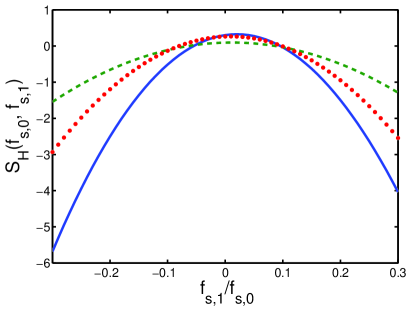
Figure 4: (color online) Function $S_{H}\left(f_{s,0},f_{s,1}\right)$, which determines the sign of the magnetic-field dependence of the spin susceptibility calculated to fourth order in the skeleton interaction [cf. Eq. (53)], plotted as a function of $f_{s,1}/f_{s,0}$ for $f_{s,0}=-0.3\;\mathrm{(dashed)},-0.5\;\mathrm{(dotted)},-0.7\;\mathrm{(dashed)}$. The curve for $f_{s,0}=-0.3$ was multiplied by a factor of 10 for clarity.

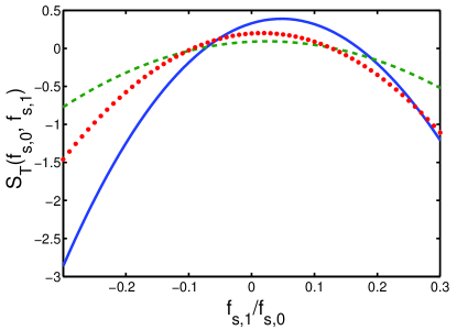
Figure 5: (color online) Function $S_{T}\left(f_{s,0},f_{s,1}\right)$, which determines the sign of the magnetic-field dependence of the spin susceptibility calculated to fourth order in the skeleton interaction [cf. Eq. (55)], plotted as a function of $f_{s,1}/f_{s,0}$ for $f_{s,0}=-0.3\;\mathrm{(dashed)},-0.5\;\mathrm{(dotted)},-0.7\;\mathrm{(solid)}$. The curve for $f_{s,0}=-0.3$ was multiplied by a factor of 10 for clarity.

A simple way to estimate the validity of the approximation used in Eqs. (57) and (58) is to consider the scattering amplitude with two rather than one components:

$$f_{s}(\phi)=f_{s,0}+f_{s,1}\cos\phi.$$ (59)

The vanishing of $f_{s}(\pi)$ at $T\to 0$ implies that $f_{s,0}=f_{s,1}$ at $T=0$. In the approximation used to derive (58), this relation was accounted for in the quadratic but not in higher-order terms. Substituting $f_{s,0}=f_{s,1}$ into the third and fourth order terms in $f_{s}$, we obtain, instead of Eq. (58),

$$\delta\chi(T,H=0) = \left[(0.02)\times\frac{2}{3}f_{s,0}^{3}+(-45.65)\times\frac{3}{4}f_{s,0}^{4}+\ldots\right]$$ (60)

$$\times\left(\frac{{\tilde{\mu}}_{B}}{\mu_{B}}\right)^{2}\frac{T}{{\tilde{\epsilon}}_{F}}\chi^{2D}_{0}$$

Comparing (60) to (58), we see that the prefactors differ substantially, making it difficult to draw a general conclusion. At the same time, the signs of both terms in (60) are negative for $f_{s,0}<0$; hence, to this order, $\delta\chi(T,H=0)<0$, which is consistent with Ref. finn_new, .

II.3.2 Coulomb interaction in the large N limit

Another issue is that the results of Refs. finn, ; finn_new, , as well as Eq. (60), are valid only below a characteristic energy scale at which Cooper renormalizations of $f_{s,0}$ become significant. For a weak interaction, this scale is exponentially small. To estimate this scale beyond the weak-coupling regime, we consider the effect of Cooper renormalization of the backscattering amplitude on the spin susceptibility in a large $N$ model for the Coulomb interaction, developed earlier in Refs. takada, ; iordanskii, ; suhas_dm, . To be specific, we assume that there are $N_{v}$ degenerate electron valleys, so that the total (spin$\times$valley) degeneracy is $N=2N_{v}$. While this model is especially relevant to Si- and AlAs-based heterostructures, which have at least two valleys ($N=4$), it can also provide a useful insight even for single-valley system ($N=2$).

In an $N$-fold degenerate 2D Fermi gas, the Fermi momentum is scaled down by a factor of $\sqrt{N}$: $k_{F}=n/\sqrt{4\pi N}$, where $n$ is the number density of electrons. On the other hand, the inverse screening radius $\kappa$, which is proportional to the density of states, is scaled up by a factor of $N$. Their ratio,

$$g_{N}=\kappa/k_{F}=r_{s}N^{3/2}/2$$ (61)

with $r_{s}=me^{2}/\sqrt{\pi n}$, defines an effective coupling constant. We still need to assume that $r_{s}\ll 1$; only then the mean-field, random-phase approximation (RPA) is valid. If $N\sim 1$, then $g_{N}\sim r_{s}\ll 1$, which implies that there is only a weak-coupling regime. If $N\gg 1$, there are two regimes: weak coupling ($g_{N}\ll 1$) and strong coupling ($g_{N}\gg 1$); the latter is of the most interest for us.

The details of the calculation are given in Appendix A. Here we present only the result for the field-dependent part of the spin susceptibility

$$\delta\chi=\frac{|\Delta|}{8\epsilon_{F}}\left(\frac{N^{2}}{L_{C}^{2}}-\frac{2}{N}\right)\chi^{2D}_{0},$$ (62)

where $L_{C}=\ln\left(\epsilon_{F}/|\Delta|\right)$ is the Cooper logarithm and, as before, $\Delta=2\mu_{B}H$. Equation (62) is valid for $L_{C}\gg 1$, i.e., for $\Delta\ll E_{C}\equiv\epsilon_{F}\exp\left(-N\right)$. The first term in Eq. (62) is the backscattering contribution, which is the leading term in the $1/N$ expansion. The second term is the contribution from other processes, which is the next-to-leading term in this expansion. As expected, the backscattering contribution is scaled down by a factor of $1/L_{C}^{2}$. The change of sign occurs at $L_{C}=N^{3/2}/\sqrt{2}$ or

$$\Delta=E^{*}=\epsilon_{F}\exp\left(-N^{3/2}/\sqrt{2}\right)\ll E_{C}.$$ (63)

For an estimate, we consider a 2D electron gas in the $(001)$ plane of a Si MOSFET, where $N=4$; correspondingly, $E_{C}=0.018\epsilon_{F}$ and $E^{*}=0.0035\epsilon_{F}$. In the experiment of Ref. reznikov, , the highest Fermi energy in this measurement is about $40$K. Then, $E_{C}=0.70$ K and $E^{*}=0.14$ K. Both energies are smaller than the disorder broadening in these samples. This shows that the mechanism of the sign reversal of $\delta\chi$ due to Cooper renormalization does not have room to develop until disorder becomes important. $\delta\chi$ in Ref.  reznikov, .

Notice also that $E_{C}$ is still larger than the energy scale of the Kohn-Luttinger superconducting instability. Indeed, in 2D the Kohn-Luttinger effect starts only at third order in the interaction, chubukov_kl which implies that $E_{KL}\sim\exp(-N^{3})\epsilon_{F}\ll E_{C}$.

The above estimates are based on additional assumptions, such as $N\gg 1$, and therefore cannot give rigorous results regarding the $T$ and $H$ dependences measured in 2D heterostructures. The crucial experimental check for the many-body nature of these effects is the $T/H$ scaling of the susceptibility which, to the best of our knowledge, has not been performed in detail.

We should also point out that while the $T$-dependence of $\chi$ in Si MOSFET was obtained in a thermodynamic measurement (via the magnetocapacitance), reznikov the $H$-dependence of $\chi$ is all heterostructures pudalov_gershenson ; stormer ; shayegan was extracted from Shubnikov-de Haas oscillations. While it is known that Shubnikov-de Haas oscillations contain a renormalized spin susceptibility of a FL, $\chi(0,0)$, it remains to be verified that the field-dependence of the susceptibility can also be extracted from such a measurement. loss_comment

II.4 Thermodynamic potential of a 2D Fermi liquid as a function of magnetization

Preparing the ground for the analysis of a ferromagnetic QCP in Sec. III, it is convenient to obtain the thermodynamic potential in terms of magnetization rather than of magnetic field. In this formulation, the susceptibility is defined as

$$\chi^{-1}=\frac{1}{\mu_{B}^{2}}\frac{\partial^{2}\Xi}{\partial M^{2}},$$ (64)

where $M=n_{\uparrow}-n_{\downarrow}$ and $n_{\uparrow/\downarrow}$ is the number density of spin-up/down fermions.

In the RPA, which neglects FL renormalizations ($Z={\tilde{v}}_{F}/v_{F}=1$), the recipe for finding the free energy was given in Ref. bealmonod68, . For a local interaction $U=u/\nu$,

$$\Xi(\Delta,M,T)=-\frac{\nu\Delta^{2}}{4}+\frac{M\Delta}{2}-\frac{uM^{2}}{4\nu}+\delta\Xi,$$ (65)

where $\delta\Xi(T,\Delta)$ is the sum of the RPA (ladder) series

$$\delta\Xi=T\sum_{q}\left(\ln\left[1+(u/\nu)\Pi_{\uparrow\downarrow}\right]-(u/\nu)\Pi_{\uparrow\downarrow}\right).$$ (66)

(The second term in Eq. (66) compensates for the first-order contribution not present in the ladder series.) The relation between $M$ and $\Delta$ is found from the condition $\left(\partial\Xi/\partial\Delta\right)\big{|}_{T,M}=0$, which gives $M=\nu\Delta$. Neglecting the RPA term, one obtains the Stoner-like spin susceptibility $\chi(0,0)=2\mu^{2}_{B}\nu/(1-u)$, which is consistent with (31) for $Z={\tilde{v}}_{F}/v_{F}=1$ and $f_{0,s}=-u/(1-u)$ (or, equivalently, $g_{s,0}=-u$). Evaluating further $\chi(T,\Delta)$ with the RPA term included, and using the relation between $\Delta$ and $M$, one reproduces Eqs. (48) and (49) without FL renormalizations.

II.4.1 Fermi-liquid renormalizations

Equation (65) can be generalized to a FL. In this Section, we assume that the system is away from the immediate vicinity of a QCP, and the effective interaction can be considered as static. We discuss specific conditions below. For a static interaction the relevant fermion self-energy depends on $k$ but not on $\omega_{m}$:

$$\Sigma^{{\mathrm{F}}}(\omega_{m},k)\approx-\left({\tilde{v}}_{F}-v_{F}\right)(k-k_{F}).$$ (67)

In this case, the quasiparticle residue $Z=\left(1-i\partial\Sigma/\partial\omega_{m}\right)^{-1}$ is equal to unity and the fermion Green’s function is given by

$$G_{\uparrow,\downarrow}(\omega_{m},k)=\frac{1}{i\omega_{m}-{\tilde{v}}_{F}(k-k_{F})\pm{\tilde{\Delta}}/2},$$ (68)

where, as before, ${\tilde{\Delta}}=2{\tilde{\mu}}_{B}H=2\mu_{B}H/(1+g_{s,0})$. We will see later in Sec. III that the self-energy becomes predominantly $\omega_{m}$- but not $k$- dependent in the immediate vicinity of a QCP.

Since our primary interest is the spin susceptibility at small momenta, we focus on the Pomeranchuk instability towards a ferromagnetic state. In the FL theory, this instability occurs when $g_{s,0}$ approaches $-1$. All other partial components of the spin and charge scattering amplitudes are assumed to remain finite at criticality and, without loss of generality, can be taken to be small.

The primary goal of the present Section is to demonstrate that some terms in the thermodynamic potential of Eq. (65) are renormalized at energies comparable to the bandwidth, where $\Sigma$ is static, while others are renormalized at much smaller energies, of order $\max\{T,M/(v_{F}\nu/{\tilde{v}}_{F})\}$, where $\Sigma^{F}$ is dynamic.

Consider first the $\Delta^{2}$ term in Eq. (65), which is the thermodynamic potential of free fermions. For a FL, this term can be calculated using the renormalized Green’s function (68). Applying the Luttinger-Ward formula LW for the thermodynamic potential of free fermions and expanding $\Xi$ to order ${\tilde{\Delta}}^{2}$, we obtain at $T=0$

$$\Xi^{(0)} = -\sum_{\sigma=\uparrow,\downarrow}\int\frac{d\omega_{m}}{2\pi}\nu\int^{W}_{-W}v_{F}d(k-k_{F})\ln\left(-G^{-1}_{\sigma}\right)$$ (69)

$$=\frac{\nu{\tilde{\Delta}}^{2}}{4}\int\frac{d\omega_{m}}{2\pi}\int^{W}_{-W}\frac{v_{F}d(k-k_{F})}{\left({\tilde{v}}_{F}(k-k_{F})-i\omega_{m}\right)^{2}}.$$

The integrals in Eq. (69) are controlled by large momenta and energies, of order $\omega_{m}\sim v_{F}|k-k_{F}|\sim W$. Integrating first over $k$ and then over $\omega_{m}$, we find that

$$\Xi^{(0)}=-\frac{v_{F}}{{\tilde{v}}_{F}}\frac{\nu{\tilde{\Delta}}^{2}}{4}.$$ (70)

To evaluate the second term in (65), we need the relation between the magnetization and Zeeman energy, which can be found by expressing the number densities of spin-up and spin-down fermions in terms of the Green’s functions

$$M = n_{\uparrow}-n_{\downarrow}$$ (71)

$$= \nu\int\frac{d\omega_{m}}{2\pi}\int^{W}_{-W}v_{F}d(k-k_{F})\left[G_{\uparrow}-G_{\downarrow}\right].$$

Using the Green’s functions from Eq. (68), we again find that the integrals in Eq. (71) are controlled by energies of order $W$. Performing the integrations, we obtain

$$M=\nu\frac{v_{F}}{{\tilde{v}}_{F}}{\tilde{\Delta}}.$$ (72)

Using (70) and recalling that the relation (72) must follow from the condition $\partial\Xi/\partial{\tilde{\Delta}}=0$, we find that the second term in (65) retains its form, but $\Delta$ changes to ${\tilde{\Delta}}$.

In a similar way, the Hubbard $U$ in the Hartree term in Eq. (65) is replaced by the Landau parameter

$$U=\frac{u}{\nu}\rightarrow-\frac{{\tilde{v}}_{F}}{v_{F}}~{}\frac{g_{s,0}}{\nu},$$ (73)

so that the Hartree term becomes

$$\frac{{\tilde{v}}_{F}g_{s,0}}{4v_{F}\nu}~{}M^{2}.$$ (74)

As a result, we have

$$\Xi(T,M,{\tilde{\Delta}})=-\frac{v_{F}}{4{\tilde{v}}_{F}}\nu{\tilde{\Delta}}^{2}+\frac{1}{2}M{\tilde{\Delta}}+\frac{{\tilde{v}}_{F}g_{s,0}}{4v_{F}\nu}M^{2}+\delta\Xi(T,{\tilde{\Delta}}).$$ (75)

So far, all renormalizations in Eq. (75) are from energies of order $W$.

Consider next the RPA term, $\delta\Xi(T,{\tilde{\Delta}})$. Re-calculating it with $G(k,\omega_{m})$ from Eq. (68), we find that it retains the same form as in Eq. (66), except that $U$ is replaced again by the Landau parameter and the polarization bubble $\Pi_{\uparrow\downarrow}$ contains the renormalized Fermi velocity:

$$\delta\Xi(T,{\tilde{\Delta}})=T\sum_{q}\left(\ln\left[1-\frac{g_{s,0}{\tilde{v}}_{F}}{v_{F}\nu}~{}\Pi_{\uparrow\downarrow}\right]+\frac{g_{s,0}{\tilde{v}}_{F}}{v_{F}\nu}\Pi_{\uparrow\downarrow}\right).$$ (76)

There are both analytic and nonanalytic terms in $\delta\Xi$. The analytic, ${\tilde{\Delta}}^{2}$ contribution comes from energies $O(W)$ and can be absorbed into the $M^{2}$ term in Eq. (75), once the prefactor is expressed in terms of the Landau parameter $g_{s,0}$ rather than of the bare interaction. The leading nonanalytic term has the same $|{\tilde{\Delta}}|^{3}$ form, as in the perturbation theory, but the prefactor now contains the FL parameters $g_{s,0}$ and $v_{F}/{\tilde{v}}_{F}$. At $T=0$,

$$\delta\Xi(0,{\tilde{\Delta}})\rightarrow-\frac{|{\tilde{\Delta}}|^{3}}{24\pi{{\tilde{v}}_{F}}^{2}}\left(\frac{f_{s,0}}{1-f_{s,0}}\right)^{2}.$$ (77)

The key point is that the ${\tilde{\Delta}}^{3}$ term in Eq. (77) comes from small energies: $\omega_{m}\sim{\tilde{v}}_{F}(k-k_{F})\sim{\tilde{\Delta}}\ll W$. Therefore, ${\tilde{v}}_{F}$ in Eq. (77) is the Fermi velocity on the small-energy scale.

The equilibrium condition $\left(\partial\Xi/\partial\Delta\right)\big{|}_{T,M}=0$ now gives $M={\tilde{\Delta}}\nu(v_{F}/{\tilde{v}}_{F})+O({\tilde{\Delta}}^{2})$, consistent with Eq. (72), and the spin susceptibility at $T=M=0$ is obtained from Eq. (64)

$$\chi(0,0)=\mu^{2}_{B}\frac{m}{\pi}~{}\frac{v_{F}}{{\tilde{v}}_{F}}~{}\frac{1}{1+g_{s,0}}=\mu^{2}_{B}\frac{m}{\pi}~{}\frac{v_{F}}{{\tilde{v}}_{F}}~{}\left(1-f_{s,0}\right).$$ (78)

As expected, this result coincides with the general expression for the renormalized spin susceptibility in a FL (Ref. agd, ).

Using Eqs. (75) and (76), we can now construct an expansion of the thermodynamic potential in powers of magnetization. To order $|M|^{3}$ and at $T=0$, we obtain

$$\Xi(T=0,M) = \frac{1}{4\nu(1-f_{s,0})}\frac{{\tilde{v}}_{F}}{v_{F}}M^{2}-\frac{1}{24\pi\nu^{3}v^{2}_{F}}\frac{{\tilde{v}}_{F}}{v_{F}}\left(\frac{f_{s,0}}{1-f_{s,0}}\right)^{2}|M|^{3}+bM^{4}+...$$ (79)

$$=\frac{1}{4\nu}\frac{{\tilde{v}}_{F}}{v_{F}}(1+g_{s,0})M^{2}-\frac{g^{2}_{s,0}}{24\pi\nu^{3}v^{2}_{F}}\frac{{\tilde{v}}_{F}}{v_{F}}|M|^{3}+bM^{4}+...$$

For completeness, we added a regular $M^{4}$ term to $\Xi$.

Evaluating $\chi(T=0,M)$ with the help of Eq. (64) and using the relation between ${\tilde{M}}$ and equilibrium ${\tilde{\Delta}}$, we reproduce the linear in $H$ term in the spin susceptibility, Eq. (48).

We emphasize again that the $M^{2}$ and $|M|^{3}$ terms in Eq. (79) come from different energy scales. The $M^{2}$ term comes from high energies of order $W$, and ${\tilde{v}}_{F}$ in this term is the renormalized Fermi velocity at energies of order $W$. The $|M|^{3}$ term comes from fermions with energies of order $M/(v_{F}\nu/{\tilde{v}}_{F})={\tilde{\Delta}}$, and ${\tilde{v}}_{F}$ in the $|M|^{3}$ term is the Fermi velocity on that scale.

At finite temperature, the expression for the thermodynamic potential becomes more involved. We present only the result and show the details of the derivation later, in Sec. (III.4.1), where we compute $\Xi(T,M)$ in the spin-fermion model. To logarithmic accuracy, we obtain

$$\Xi(T,M) = \frac{M^{2}}{4\nu}\frac{{\tilde{v}}_{F}}{v_{F}}\left[(1-f_{s,0})^{-1}-\left(\frac{f_{s,0}}{1-f_{s,0}}+\ln(1-f_{s,0})\right)\frac{{\tilde{v}}_{F}}{v_{F}}\frac{T}{\epsilon_{F}}\right]-\left(\frac{f_{s,0}}{1-f_{s,0}}\right)^{2}\frac{M^{4}}{576\pi T\nu^{4}v^{2}_{F}}\left(\frac{{\tilde{v}}_{F}}{v_{F}}\right)^{2}+bM^{4}+...$$ (80)

$$=\frac{M^{2}}{4\nu}\frac{{\tilde{v}}_{F}}{v_{F}}\left[1+g_{s,0}-\left(g_{s,0}+\ln(1+g_{s,0})^{-1}\right)\frac{{\tilde{v}}_{F}}{v_{F}}\frac{T}{\epsilon_{F}}\right]-\frac{g^{2}_{s,0}M^{4}}{576\pi T\nu^{4}v^{2}_{F}}\left(\frac{{\tilde{v}}_{F}}{v_{F}}\right)^{2}+bM^{4}+...$$

The key result here is that for $T\gg M/(v_{F}\nu/{\tilde{v}}_{F})$ the expansion of $\Xi$ in powers of $M$ becomes analytic: the $|M|^{3}$ term is replaced by an analytic $M^{4}/T$ term. Simultaneously, the prefactor for the quadratic term acquires a linear in $T$ correction, which is just a nonanalytic temperature dependence of the spin susceptibility. Indeed, evaluating $\chi(T,0)$, from (80), we reproduce Eq. (49).

III Magnetic response near a 2D ferromagnetic quantum critical point

III.1 General considerations

We now consider the immediate vicinity of a ferromagnetic QCP. In what follows, we first assume that a continuous ferromagnetic transition does exists and obtain the thermodynamic potential $\Xi(M,T)$ along a continuous second-order transition line by extending Eqs. (79) and (80) to energies below the scale where the self-energy crosses from static to dynamic forms. (chub_cross, ; cgy, ). Next, we show that this line becomes unstable at low enough temperatures because of nonanalyticities which survive even in the vicinity of the QCP. We will argue that the instability may occur in two ways: i) the second-order phase transition into a uniform ferromagnetic phase becomes first order or ii) the transition occurs via an intermediate magnetic phase with a spiral magnetic order. More specific predictions are possible within more specific models. One of such models is a model with a large radius of the interaction in the spin channel. dzero We will show that in this model the first-order instability occurs before the spiral one.

A tendency towards the first-order transition can be seen already from Eq. (79). Indeed, the cubic term in $M$ in $\Xi(M,T=0)$ is negative, which implies that a state with finite magnetization is energetically favorable. Close to the critical point, the $M^{2}$ term is small and the thermodynamic potential (79) is negative over some range of $M$. This means that the first-order phase transition preempts the second-order one at $T=0$. Indeed, for the thermodynamic potential of the form

$$\Xi(M)=aM^{2}-c|M|^{3}+bM^{4}$$ (81)

with $c>0$, the magnetization jumps to finite value of $M_{0}=2a/c$ already for $a=c^{2}/4b>0$, i.e., before the second-order transition takes place.

At finite $T$, the $|M|^{3}$ term in the thermodynamic potential crosses over into a $-M^{4}/T$ one, which is still negative. If $T$ is low enough, this negative term is larger than the regular, $M^{4}$ term, and the transition remains first order until the $-M^{4}/T$ term becomes smaller than the regular $bM^{4}$ term. At higher $T$, the transition becomes second-order.

This analysis is, however, incomplete because it is based on the result for $\Xi(T.M)$ derived under assumptions that the quasiparticle residue $Z=1$ and the effective Fermi velocity ${\tilde{v}}_{F}=k_{F}/m^{*}$ is finite. As we have already mentioned, this is true only if the self-energy is static. Since the first-order jump in magnetization, $M_{0}$, is proportional to the critical parameter $1+g_{s,0}$, the corresponding energy scale $M_{0}/\nu$ is also small and falls into the regime where the self-energy is dynamic and Eq. (79) is no longer valid.

If the self-energy is dynamic, the $Z$ factor and ${\tilde{v}}_{F}/v_{F}$ are both given by $\left(1-i\partial\Sigma(\omega_{m})/\partial\omega_{m}\right)^{-1}$ (so that the product $Zv_{F}/{\tilde{v}}_{F}$ remains intact.) This would not lead to substantial changes if $Z$ remained finite at a QCP. However, it is well established by now that $\partial\Sigma(\omega_{m})/\partial\omega_{m}$ diverges at a ferromagnetic QCP in 2D; hence, both $Z$ and ${\tilde{v}}_{F}/v_{F}$ vanish. aim ; 2/3 ; chub_cross ; rosch_rmp ; pepin_prl ; pepin_prb One then might be tempted to conclude that the nonanalytic term in Eq. (79) vanishes, as it is proportional as an overall factor to the renormalized velocity ${\tilde{v}}_{F}$ evaluated at low energies. We will show, however, that the nonanalytic term in the free energy survives even at the QCP, albeit in a weaker form ($|M|^{3}$ is replaced by $|M|^{7/2}$).

Before proceeding further, we mention two paradoxes with the vanishing of $Z$ and ${\tilde{v}}_{F}/v_{F}$ at a ferromagnetic QCP. First, there seems to be a contradiction with the Stoner criterion which says that a ferromagnetic transition occurs at some critical, finite interaction strength. If we formally use the FL relation $g_{s,0}=Z(Zv_{F}/{\tilde{v}}_{F})\Gamma^{\Omega}$ (Ref. agd, ) with $Z\rightarrow 0$ but $Zv_{F}/{\tilde{v}}_{F}=\text{const}$, we find that the condition $g_{s,0}=-1$ can be satisfied only if $\Gamma^{\Omega}\to\infty$. Second, in the FL theory, the velocity renormalization is determined by the $l=1$ harmonic of the Landau function in the charge sector: $v/{\tilde{v}}_{F}={\tilde{m}}/m=1+g_{c,1}$. Hence, the vanishing of ${\tilde{v}}_{F}$ implies that $g_{c,1}=\infty$. Meanwhile, the very idea of a Pomeranchuk instability is that it occurs only in one particular channel, e.g., in the spin channel with the angular momentum $l=0$ for a ferromagnetic QCP. All other channels, including the charge channel with $l=1$, remain uncritical, which seems to be inconsistent with the condition $g_{c,1}=\infty$.

We make a few general remarks about these two paradoxes first and show specific results later.

• The assumption of the conventional FL theory about a single relevant $l=0$ spin channel near a ferromagnetic QCP is valid if there is a wide range of energies below the cutoff $W$, where the fermion self-energy is static. Within this range, $Z=1$ and $v_{F}/{\tilde{v}}_{F}$ differs from its bare value only because of a non-singular interaction in the $l=1$ channel. Then $g_{s,0}=Z^{2}(v_{F}/{\tilde{v}}_{F})\nu\Gamma^{\Omega}$ is of the same order as $\nu\Gamma^{\Omega}$, and a critical value of $g_{s,0}=-1$ is approached already at finite interaction strength. As we have already demonstrated, the Stoner enhancement of the spin susceptibility comes from fermions with energies of order $W$, hence, at energies below $W$, the susceptibility is already enhanced by the Stoner factor $(1+g_{s,0})^{-1}>1$.

• At some energy scale, $\Lambda<W$, the self-energy undergoes a crossover between static and dynamic forms. Accordingly, $Z$ and $v_{F}/{\tilde{v}}_{F}$ begin to vary below $\Lambda$ and eventually flow to zero at the QCP. In this regime, the conventional FL theory based on the static approximation is no longer valid and has to be replaced by a “new” low-energy FL theory, in which the “bare” fermions are the ones on the scale of $\Lambda$, the “bare” interaction between fermions is in the spin channel, and the interaction potential $U$ is replaced by the effective interaction, which scales as $1/(1+g_{s,0})$. This low-energy FL theory is a spin-fermion model. The Landau parameters for the low-energy FL differ from those of the conventional FL. In particular, all harmonics $g_{c,l}$, including $g_{c,1}=v_{F}/{\tilde{v}}_{F}-1$ diverge at a 2D QCP. we_new

• The spin-fermion model is valid only if the crossover between static and dynamic forms of the self-energy occurs on a scale much smaller than $W$. Otherwise, one cannot consider only the $l=0$ spin channel. As we will see, the condition $\Lambda\ll W$ can be satisfied if the interaction is sufficiently long-range or, else, if the model is extended to $N\gg 1$ fermion flavors. We will assume below that at least one of these two conditions is satisfied.

Because both $Z$ and $v_{F}/{\tilde{v}}_{F}$ on the scale of $\Lambda$ are just constants, we will absorb $Z$ into the effective spin interaction, and measure the velocity renormalization below the cutoff with respect to its value at the cutoff. In other words, we assume that the bare fermion propagator is $G^{-1}(k,\omega_{m})=i\omega_{m}-v_{F}(k-k_{F})$, and use symbols $Z$ and ${\tilde{v}}_{F}$ to describe renormalizations at energies smaller than $\Lambda$.

III.2 Spin-fermion model in zero magnetic field

We now consider in detail the low-energy effective theory near a ferromagnetic QCP: the spin-fermion model We first review briefly the properties of this model in zero magnetic field pepin_prb and then show how the model is modified in the presence of the field.

The spin-fermion model includes low-energy fermions with a bare propagator $G(k,\omega_{m})$, collective spin excitations ${\mathbf{S}}_{{\mathbf{q}}}$, whose bare propagator is the static spin susceptibility $\chi(q)$, and the spin-fermion interaction, described by the Hamiltonian

$$H_{int}=\frac{g}{{\cal N}}\sum_{\mathbf{k},\mathbf{q},\alpha,\alpha^{\prime}}c^{\dagger}_{\mathbf{k},\alpha}{\vec{\sigma}}_{\alpha,\alpha^{\prime}}\cdot\mathbf{S}_{\mathbf{q}}c_{\mathbf{k}+\mathbf{q},\alpha^{\prime}},$$ (82)

where ${\cal N}$ is the number of lattice sites. The spin-fermion coupling $g$ is related to the Landau parameter $g_{s,0}$ as $g=(\pi/m)\sqrt{-g_{s,0}}$. Near the QCP, $g_{s,0}\approx-1$ and $g\approx\pi/m$. The bare boson propagator $\chi(q)$ is proportional to $1/(1+g_{s,0})$ for $q\to 0$. We assume that the $q$ dependence of $\chi$ at small but finite $q$ is described by the standard Ornstein-Zernike formula

$$\chi(q)=\frac{m}{\pi}~{}\frac{1}{1+g_{s,0}+(aq)^{2}}=\frac{m}{\pi a^{2}}~{}\frac{1}{\xi^{-2}+q^{2}},$$ (83)

where

$$\xi^{-2}=(1+g_{s,0})a^{-2}.$$ (84)

Similar to the $1+g_{s,0}$ term, the analytic $q^{2}$ term in $\chi(q)$ comes from fermions with energies comparable to $W$. This term can be obtained in the RPA scheme, but one has to assume either that the dispersion is different from a free-fermion one, i.e., from $k^{2}/2m$, or that the exchange interaction is momentum-dependent; otherwise the particle-hole polarization bubble does not depend on $q$ for $q\leq 2k_{F}$ in 2D. If the $q^{2}$ term is comes from the momentum dependence of the interaction, the length $a$ is the radius of the interaction. In this case, the RPA is justified for a sufficiently long-ranged interaction, i.e., for $ak_{F}\gg 1$ (Ref. dzero, .)

The spin-fermion interaction affects both fermion and boson propagators. Collective spin excitations acquire a self-energy $\Sigma^{{\mathrm{B}}}(q,\Omega)$, while fermions acquire a self-energy $\Sigma^{{\rm F}}(k,\omega_{m})$ which gives rise to renormalizations of $Z$ and of the Fermi velocity:

$$G(k,\omega_{m})=\frac{1}{i\omega_{m}-v_{F}(k-k_{F})+\Sigma^{{\mathrm{F}}}(k,\omega_{m})}$$

$$\chi(q,\Omega_{m})=\frac{m}{\pi}~{}\frac{1}{1+g_{s,0}+(aq)^{2}+\Sigma^{{\mathrm{B}}}(q,\Omega_{m})}.$$ (85)

To one-loop order, the $T=0$ self-energies behave as

$$\Sigma^{{\mathrm{B}}}={\tilde{g}}^{2}\frac{\Omega_{m}}{v_{F}q}$$

$$\Sigma^{{\mathrm{F}}}(k=k_{F},\omega_{m})=\left\{\begin{array}[]{lcl}i\lambda~{}\omega_{m},&\mbox{~{}for~{}}&\omega_{m}\ll\omega_{0}/\lambda^{3},\\ i\omega_{0}^{1/3}\omega_{m}^{2/3},&\mbox{~{}for~{}}&\omega_{0}/\lambda^{3}\ll\omega_{m}\ll\omega_{\max}\sim\omega^{1/4}_{0}\ \epsilon^{3/4}_{F}\end{array}\right.$$ (87)

$$\Sigma^{{\mathrm{F}}}(k,\omega_{m}=0)\sim v_{F}(k-k_{F})\left(\frac{\omega_{0}}{\varepsilon_{F}}\right)^{1/4}\times{\cal S}\left(\frac{\lambda}{\tilde{g}}\right)$$ (88)

where

$$\omega_{0}=\varepsilon_{F}\frac{3\sqrt{3}}{4}\left(\frac{{\tilde{g}}}{ak_{F}}\right)^{4},\;~{}~{}\lambda=\frac{3{\tilde{g}}^{2}}{4ak_{F}}~{}\frac{1}{\sqrt{1+g_{s,0}}},~{}~{}{\tilde{g}}=2g\nu\approx\frac{mg}{\pi},$$ (89)

and ${\cal S}(x\ll 1)\sim x,~{}~{}{\cal S}(x\gg 1)=O(1)$. To simplify the formulas, we assume that $\omega_{m}>0$. Eq. (88) is valid for $\omega_{0}/\lambda^{3}\ll\omega_{\max}$, i.e., for $\delta\ll 1$.

In the RPA, a ferromagnetic transition occurs at ${\tilde{g}}=1$, but the critical value of ${\tilde{g}}$ may differ from one in a more general model. For $ak_{F}\gg 1$, $\omega_{0}$ is parametrically small compared to $\epsilon_{F}$, i.e., the $k-$dependent part of the self-energy is always smaller than $v_{F}(k-k_{F})$.

To compare the frequency- and momentum-dependences of the self-energy, we consider the Green’s function near the renormalized mass shell: $v_{F}(k-k_{F})=i\omega_{m}+\Sigma_{{\mathrm{F}}}(k,\omega_{m})$. For $\omega_{m}\ll\omega_{0}$, $i\omega_{m}\ll\Sigma_{{\mathrm{F}}}$ and $v_{F}|k-k_{F}|\sim\omega^{2/3}\omega_{0}^{1/3}$ near the mass shell. Consequently, the $k$-dependent part of the self-energy is smaller than the $\omega_{m}$-dependent part. For $\omega_{m}\gg\omega_{0}$, $\Sigma^{{\mathrm{F}}}(\omega_{m})\ll i\omega_{m}$ and $\epsilon_{k}v_{F}|k-k_{F}|\sim\omega_{m}$ near the mass shell. Comparing $\Sigma^{{\mathrm{F}}}(k,\omega_{m}=0)$ and $\Sigma^{{\mathrm{F}}}(k=k_{F},\omega_{m})$, we find that the two become comparable at $\omega_{m}\sim\omega_{\max}=\omega_{0}\left(\epsilon_{F}/\omega_{0}\right)^{3/4}$. For $\omega_{m}\ll\omega_{\max}$, $\Sigma^{{\mathrm{F}}}(k,\omega_{m})$ depends predominantly on $\omega_{m}$ while for $\omega_{m}\gg\omega_{\max}$ it depends predominantly on $k$. Note that $\omega_{\max}$ is also the upper cutoff for $\omega_{m}^{2/3}$ scaling of the fermion self-energy (see Eq. (88)]. At larger $\omega_{m}$, $\Sigma^{F}$ scales as $\ln\omega_{m}$.

The scale $\omega_{\max}$ is larger than $\omega_{0}$ but still parametrically smaller than $\epsilon_{F}$ [indeed, $\omega_{\max}\sim\omega_{0}(ak_{F})^{3}\sim\epsilon_{F}/(ak_{F})$]. The upper limit for the low-energy theory, $\Lambda$, can then be set somewhere in between $\omega_{\max}$ and $W\sim\epsilon_{F}$; its precise location being irrelevant as long as $\omega_{\max}\ll\epsilon_{F}$.

In what follows, we will also need the fermion self-energy at finite temperatures. At finite $T$, the fermions interact both with classical ($\Omega_{m}=0$) and quantum ($\Omega_{m}\neq 0$) spin fluctuations. The quantum contribution to the self-energy is a scaling function of $\omega_{m}/T$:

$$\Sigma^{\mathrm{F}}_{\mathrm{Q}}(\omega_{m},T)=i\omega_{0}^{1/3}\omega_{m}^{2/3}Q(\omega_{m}/T),$$ (90)

where the scaling function $Q(x)$ is such that $Q(x\gg 1)=1$ and $Q(x\ll 1)\sim 1/x^{2/3}$. The classical contribution contains a static propagator that diverges at QCP as $q^{-2}$. This divergence can be regularized in two ways: by accounting for a thermally generated mass of spin fluctuations due to mode-mode coupling (not present in the spin-fermion model) millis_qcp ; delanna or by resumming the self-consistent Born series.abanov_ch In the first approach, the zero-temperature correlation length in Eq. (83) $\xi(0)=a/\sqrt{1+g_{s,0}}$ is replaced by $\xi(T)\sim a/\left[\left(T/\Lambda\right)\ln\left(\Lambda/T\right)\right]^{1/2}$ (Ref. millis_qcp, ). The classical part of the self-energy $\Sigma^{\mathrm{F}}_{\mathrm{C}}\equiv\Sigma^{\mathrm{F}}\left(\omega_{m}=\pi T,T\right)$ then becomes

$$\Sigma^{\mathrm{F}}_{\mathrm{C}}=i\frac{3}{4}{\tilde{g}}T\frac{\xi(T)}{k_{F}a^{2}}\propto i\left(\frac{T}{\ln\left(\Lambda/T\right)}\right)^{1/2}.$$ (91)

In the second approach, one obtains a self-consistent equation for $\Sigma$ which yields a similar $T$ dependence of $\Sigma^{\mathrm{F}}_{T}$.

The quantum and classical contributions become comparable at a characteristic temperature

$$T_{\mathrm{QC}}={\tilde{g}}^{6}\left(ak_{F}\right)^{2}\frac{\Lambda^{3}}{\epsilon_{F}^{2}}.$$ (92)

For $T\ll T_{\mathrm{QC}}$ the classical contribution dominates over the quantum one, and vice versa.

III.2.1 Eliashberg theory

We now focus on the low-energy region $\omega_{m}\ll\omega_{\max}$, where $\Sigma^{{\mathrm{F}}}(k,\omega_{m})$ is predominantly dynamic. Within this region, there exists another scale, $\omega_{0}\sim\omega_{\max}/(ak_{F})^{3}\ll\omega_{\max}$, at which the fermion self-energy becomes comparable to $\omega_{m}$. Below $\omega_{0}$, $\Sigma^{{\mathrm{F}}}(\omega_{m})>\omega_{m}$, i.e., the system is in a strong-coupling regime. Close enough to the QCP, i.e., for $\lambda\gg 1$, the strong-coupling regime, on its turn, is divided into two more subregimes: i) $\omega_{0}/\lambda^{3}<\omega_{m}<\omega_{0}$, where the self-energy has a non-FL, $\omega_{m}^{2/3}$, form and ii) $\omega_{m}<\omega_{0}/\lambda^{3}$, where the FL behavior is restored, i.e., $\mathrm{Re}\Sigma^{{\mathrm{F}}}(\omega)\propto\omega$ and $\mathrm{Im}\Sigma^{{\mathrm{F}}}(\omega)\propto\omega^{2}$.

Since $\Sigma^{{\mathrm{F}}}(\omega_{m})>\omega_{m}$ at $\omega_{m}<\omega_{0}$, the accuracy of the one-loop approximation for the self-energy becomes an issue. Previous work aim ; pepin_prb demonstrated that the self-consistent one-loop approximation (the Eliashberg theory) cannot be controlled just by a large value of the parameter $ak_{F}$, as higher-order diagrams in the strong-coupling regime are of the same order in $1/ak_{F}$ as the one-loop diagram. To put the theory firmly under control, one needs to extend it formally to $N\gg 1$ fermion flavors; then higher order terms in the self-energy terms are small in $(\ln N)/N^{2}$. In what follows, we neglect this subtlety and assume that the Eliashberg theory is valid.

The frequency-dependent self-energy $\Sigma^{{\mathrm{F}}}(\omega_{m})$ from Eq. (88) leads to the renormalization of the $Z$-factor (equal to the inverse velocity renormalization factor). Right at the QCP, both $Z$ and $v_{F}/{\tilde{v}}_{F}$ depend on $\omega_{m}$ as

$$Z=\frac{{\tilde{v}}_{F}}{v_{F}}=\left(1-i\frac{\partial\Sigma^{F}(\omega_{m})}{\partial\omega_{m}}\right)^{-1}=\left(1+\left(\frac{\omega_{0}}{\omega_{m}}\right)^{1/3}\right)^{-1}.$$ (93)

The boson self-energy is generated by inserting the dynamic fermion bubbles, made out full propagators, into the bare spin-fermion interaction. Summing up the RPA series for the renormalized spin-fermion interaction, we obtain

$$\Sigma^{{\mathrm{B}}}(q,\Omega_{m})={\tilde{g}}^{2}~{}{\tilde{P}}(q,\Omega_{m}),$$ (94a)

$${\tilde{P}}(q,\Omega_{m})=\frac{|\Omega_{m}|}{\left[\left(\Omega_{m}-ic_{\Omega}\Sigma^{{\mathrm{F}}}(\Omega_{m})\right)^{2}+v^{2}_{F}q^{2}\right]^{1/2}},$$ (94b)

where $c_{\Omega}$ is a slowly varying function of $\Omega_{m}$, which interpolates between two limits: $c_{0}=1$ for $\Omega_{m}\ll\omega_{0}/\lambda^{3}$ and $c_{\Omega}\approx 1.2$ for $\omega_{0}/\lambda^{3}\ll\Omega_{m}\ll\omega_{0}$ (Refs. pepin_prb, ; we_short, ; bec, ). For free fermions, ${\tilde{P}}$ is the same as $P$ introduced in Eq. (5).

In the limit of small frequencies, ${\tilde{P}}(q,\Omega_{m})$ reduces to the Landau damping form $\Omega_{m}/v_{F}q$. The static boson self-energy is small in $1/(ak_{F})$ and non-singular, and we neglect it.

Equation (94b) has to be treated with caution because ${\tilde{P}}$ is the dynamic part of the particle-hole bubble made of dressed fermions but without vertex corrections. The latter are irrelevant for $v_{F}q\gg\Omega$ but are important for $v_{F}q\ll\Omega$, as they are necessary for the Ward identities to be satisfied. This problem is generic to all models in which the effective interaction is peaked at zero momentum transfer. chub_ward Fortunately, this complication does not arise in the study of non-analyticities in the thermodynamic potential and in the spin susceptibility because, as it will be shown later, we will only need to know ${\tilde{P}}(q,\Omega_{m})$ for $v_{F}q\gg\Omega_{m},\Sigma(\Omega_{m})$. Therefore, we will be using Eq. (94b) in what follows.

The thermodynamic potential of the spin-fermion model in the Eliashberg approximation was obtained in Ref. chmgg_prb, (see also Sec. III.3):

$$\Xi\left(T\right)=\Xi_{{\rm F}}\left(T\right)+\frac{3}{2}T\sum_{\Omega_{m}}\int\frac{d^{2}q}{4\pi^{2}}~{}\ln\left[\chi^{-1}\left(q,\Omega_{m}\right)\right],$$ (95)

where $\Xi_{{\rm F}}\left(T\right)=-\nu T\sum_{\omega_{m}}|\omega_{m}|=-\pi^{2}\nu T^{2}/3$ is the $T$-dependent part of the thermodynamic potential of a free Fermi gas and $\chi(q,\Omega_{m})$ is given by Eq. (85). Differentiating $\Xi(T)$ with respect to temperature, one obtains the specific heat $C(T)$, which behaves as $(1+\lambda)T$ away from the QCP and as $T^{2/3}$ at the QCP.

III.3 Spin-fermion model in a magnetic field

We now return to our main discussion and consider the spin-fermion model in the presence of a magnetic field. First, we derive a general expression for the thermodynamic potential in a magnetic field, and then analyze the structure of the nonanalytic terms in the vicinity of a ferromagnetic QCP. For reasons already explained in Sec.III.1, we take the bare fermion propagator as

$$G^{0}_{\uparrow,\downarrow}(k,\omega_{m})=\frac{1}{i\omega_{m}-v_{F}(k-k_{F})\pm{\tilde{\Delta}}/2},$$ (96)

where ${\tilde{\Delta}}=2{\tilde{\mu}}_{B}H$, and ${\tilde{\mu}}_{B}=\mu_{B}/(1+g_{s,0})$.

III.3.1 The Luttinger-Ward functional in a magnetic field

We first derive the thermodynamic potential for the spin-fermion model in finite magnetic field, starting from the Luttinger-Ward functional LW and making use of the Eliashberg approximation, which neglects vertex corrections. eliashberg ; bardeen ; prange ; chubukov_eliash ; chmgg_prb

The Luttinger-Ward functionalLW contains four terms

$$\Xi(M,{\tilde{\Delta}},T)=\Xi_{{\rm F}}+\Xi_{{\rm B}}+\Xi_{{\rm FB}}+\Xi_{M},$$ (97)

where $\Xi_{{\rm F}}$ is the potential of fermions dressed by the interaction with bosons, $\Xi_{{\rm B}}$ is the potential of bosons dressed by the interaction with fermions, $\Xi_{{\rm FB}}$ is the skeleton part which describes explicitly the fermion-boson interaction at low-energies, and $\Xi_{M}=g_{s,0}M^{2}/(4\nu)+(1/2)M{\tilde{\Delta}}$ is an extra $M$-dependent high-energy contribution, same as in (75). (There is no double counting, as one can verify explicitly.) For $H=0$, the Eliashberg form of the Luttinger-Ward functional was derived in Refs. eliashberg, ; bardeen, ; chubukov_eliash, ; chmgg_prb, . Extending the derivation to the case of finite spin polarization, we obtain

$$\Xi_{{\rm F}} = -T\sum_{k,\sigma}\left[\ln\left\{-G_{\sigma}^{-1}\left(k\right)/W\right\}-\Sigma^{{\mathrm{F}}}_{\sigma}\left(k\right)G_{\sigma}\left(k\right)\right]$$

$$\Xi_{{\rm B}} = \frac{T}{4}\sum_{q,\sigma,\sigma^{\prime}}\left(1+\delta_{\sigma,\sigma^{\prime}}\right)\left[\ln\left\{D_{\sigma,\sigma^{\prime}}^{-1}\left(q\right)\right\}-\Sigma^{{\mathrm{B}}}_{\sigma\sigma^{\prime}}\left(q\right)D_{\sigma\sigma^{\prime}}\left(q\right)\right]$$

$$\Xi_{{\rm FB}} = \frac{{\tilde{g}}^{2}}{4\nu}T^{2}\sum_{kk^{\prime},\sigma,\sigma^{\prime}}\left(1+\delta_{\sigma,\sigma^{\prime}}\right)G_{\sigma}\left(k\right)D_{\sigma\sigma^{\prime}}\left(k-k^{\prime}\right)G_{\sigma^{\prime}}\left(k^{\prime}\right),$$ (98)

where ${\tilde{g}}$ is the dimensionless coupling constant defined in Eq.  (89), $k\equiv\left(\mathbf{k},\omega_{m}\right),q\equiv\left(\mathbf{q},\Omega_{m}\right)$, $\sigma,\sigma^{\prime}=\uparrow,\downarrow$, and as before, summation over $k$ and $q$ implies summation over Matsubara frequencies and integration over momenta. The functions $G_{\uparrow,\downarrow}$ are the exact fermion Green’s function

$$G_{\uparrow,\downarrow}=\left(i\omega_{m}+\Sigma^{{\mathrm{F}}}_{\uparrow,\downarrow}\left(\omega_{m}\right)-\epsilon_{k}\pm{\tilde{\Delta}}/2\right)^{-1}$$ (99)

and $D_{\sigma\sigma^{\prime}}\left(q\right)$ is the propagator of spin fluctuations

$$D^{-1}_{\sigma,\sigma^{\prime}}\left(q\right)=1+g_{s,0}+(aq)^{2}+\Sigma^{{\mathrm{B}}}_{\sigma\sigma^{\prime}}\left(q\right),$$ (100)

where $\Sigma^{{\mathrm{F}}}_{\sigma}$ and $\Sigma^{{\mathrm{B}}}_{\sigma\sigma^{\prime}}$ are the fermion and boson self-energies, correspondingly. Notice that the fermion self-energy does not contain a constant part evaluated at $\omega_{m}=0$ and $k=k_{F}$– this part has been absorbed into the renormalized Zeeman energy, ${\tilde{\Delta}}$.

By construction, the Luttinger-Ward functional is stationary with respect to variations of the fermion and boson self-energies. The stationarity conditions

$$\frac{\delta\Xi}{\delta\Sigma_{\sigma}^{\mathrm{F}}}=\frac{\delta\Xi}{\delta\Sigma^{{\mathrm{B}}}_{\sigma,\sigma^{\prime}}}=0$$ (101)

yield

$$\Sigma^{{\mathrm{B}}}_{\sigma\sigma^{\prime}}\left(q\right) = \frac{{\tilde{g}}^{2}}{\nu}T\sum_{k}G_{\sigma}\left(k+q\right)G_{\sigma^{\prime}}\left(k\right),$$ (102a)

$$\Sigma^{{\mathrm{F}}}_{\sigma}\left(k\right) = -\frac{{\tilde{g}}^{2}}{\nu}T\sum_{q}D_{\sigma,\sigma}\left(q\right)G_{\sigma}\left(k+q\right)-\frac{{\tilde{g}}^{2}}{4\nu}T\sum_{q}\left[D_{\sigma,-\sigma}(q)+D_{-\sigma,\sigma}(q)\right]G_{-\sigma}\left(k+q\right).$$ (102b)

In the presence of a magnetic field, there are two different boson self-energies: $\Sigma^{{\mathrm{B}}}_{\uparrow\uparrow}=\Sigma^{{\mathrm{B}}}_{\downarrow\downarrow}$ and $\Sigma^{{\mathrm{B}}}_{\uparrow\downarrow}=\Sigma^{{\mathrm{B}}}_{\downarrow\uparrow}$. $\Sigma^{{\mathrm{B}}}_{\uparrow\uparrow}$ is composed of fermions of the same spin ($\Sigma^{{\mathrm{B}}}_{\uparrow\uparrow}=\Sigma^{{\mathrm{B}}}_{\downarrow\downarrow}$). It depends on the magnetization only via a shift of the chemical potential. This is a regular, analytic dependence which does not lead to nonanalyticities in the thermodynamic potential. Neglecting this dependence, we set $\Sigma^{{\mathrm{B}}}_{\uparrow\uparrow}=\Sigma^{{\mathrm{B}}}_{\downarrow\downarrow}\equiv\Sigma^{{\mathrm{B}}}$, where $\Sigma^{{\mathrm{B}}}$ is the boson self-energy in zero field, given by Eq. (94a). On the other hand, $\Sigma^{{\mathrm{B}}}_{\uparrow\downarrow}$ is composed of fermions with opposite spins and depends strongly on the magnetization via the Zeeman term: $\Sigma^{{\mathrm{B}}}_{\uparrow\downarrow}=\Sigma_{\downarrow\uparrow}^{B}={\tilde{g}}^{2}{\tilde{P}}_{\uparrow\downarrow}$, where

$${\tilde{P}}_{\uparrow\downarrow}\left(q,\Omega_{m}\right)=\frac{\left|\Omega_{m}\right|}{\sqrt{\left(\Omega_{m}-ic_{\Omega}\Sigma^{{\mathrm{F}}}(\Omega_{m})-i{\tilde{\Delta}}\right)^{2}+v_{F}^{2}q^{2}}}.$$ (103)

This also implies that $D_{\uparrow,\uparrow}(q)=D_{\downarrow,\downarrow}(q)\equiv D(q)$ and $D_{\uparrow,\downarrow}(q)=D_{\downarrow,\uparrow}(q)$. Expressions for $\Xi_{\mathrm{B}}$ and $\Xi_{\mathrm{FB}}$ can be then simplified to

$$\Xi_{{\rm B}} = T\sum_{q}\left[\ln\left\{D^{-1}\left(q\right)\right\}-\Sigma^{{\mathrm{B}}}\left(q\right)D\left(q\right)\right]+\frac{T}{2}\sum_{q}\left[\ln\left\{D_{\uparrow\downarrow}^{-1}\left(q\right)\right\}-\Sigma^{{\mathrm{B}}}_{\uparrow\downarrow}\left(q\right)D_{\uparrow\downarrow}\left(q\right)\right]$$ (104)

$$\Xi_{{\rm FB}} = \frac{{\tilde{g}}^{2}}{2\nu}T^{2}\sum_{kk^{\prime}}\left[\sum_{\sigma}D\left(k-k^{\prime}\right)G_{\sigma}\left(k\right)G_{\sigma}\left(k^{\prime}\right)+D_{\uparrow\downarrow}\left(k-k^{\prime}\right)G_{\uparrow}\left(k\right)G_{\downarrow}\left(k^{\prime}\right)\right],$$ (105)

while the fermion self-energy changes to

$$\Sigma^{{\mathrm{F}}}_{\sigma}\left(k\right)=-\frac{{\tilde{g}}^{2}}{\nu}T\sum_{q}D\left(q\right)G_{\sigma}\left(k+q\right)-\frac{{\tilde{g}}^{2}}{2\nu}T\sum_{q}D_{\uparrow\downarrow}(q)G_{-\sigma}\left(k+q\right).$$ (106)

The field-dependent part of the thermodynamic potential involves only $D_{\uparrow\downarrow}\left(q\right)$

$$\Xi = -T\sum_{k,\sigma}\left[\ln\left\{-G_{\sigma}^{-1}\left(k\right)/W\right\}-\Sigma^{{\mathrm{F}}}_{\sigma}\left(k\right)G_{\sigma}\left(k\right)\right]+\frac{T}{2}\sum_{q}\left[\ln D_{{}_{\uparrow\downarrow}}^{-1}\left(q\right)-\Sigma^{{\mathrm{B}}}_{\uparrow\downarrow}\left(q\right)D_{\uparrow\downarrow}\left(q\right)\right]$$

$$+\frac{{\tilde{g}}^{2}}{2\nu}T^{2}\sum_{kk^{\prime}}D_{\uparrow\downarrow}\left(k-k^{\prime}\right)G_{\uparrow}\left(k\right)G_{\downarrow}\left(k^{\prime}\right)+g_{s,0}\frac{M^{2}}{4\nu}+\frac{1}{2}M{\tilde{\Delta}}.$$

With the help of Eq. (102a), we simplify Eq. (III.3.1) to

$$\Xi=+g_{s,0}\frac{M^{2}}{4\nu}+\frac{1}{2}M{\tilde{\Delta}}-T\sum_{k,\sigma}\left[\ln\left\{-G_{\sigma}^{-1}\left(k\right)/W\right\}-\Sigma^{{\mathrm{F}}}_{\sigma}\left(k\right)G_{\sigma}\left(k\right)\right]+\frac{T}{2}\sum_{q}\ln D_{{}_{\uparrow\downarrow}}^{-1}\left(q\right).$$ (108)

The first two terms in Eq.(108) need to be expanded to order $\tilde{\Delta}^{2}.$ In the first, logarithmic term, we proceed in the same way as in Eq. (69). Keeping only the ${\tilde{\Delta}}^{2}$ term, we obtain

$$-T\sum_{k,\sigma}\ln\left(-G_{\sigma}^{-1}\left(k\right)/W\right)=\frac{\nu\tilde{\Delta}^{2}}{4}\int\frac{d\omega_{m}}{2\pi}\int_{-\Lambda}^{\Lambda}\frac{v_{F}d\left(k-k_{F}\right)}{\left(v_{F}\left(k-k_{F}\right)-i\tilde{\omega}_{m}\right)^{2}}=-\frac{\nu\tilde{\Delta}^{2}}{2}\int\frac{d\omega_{m}}{2\pi}\frac{\Lambda}{\tilde{\omega}_{m}^{2}+\Lambda^{2}},$$ (109)

where $\tilde{\omega}_{m}=\omega_{m}-i\Sigma^{{\mathrm{F}}}\left(\omega_{m}\right).$ The integral is controlled by frequencies $O\left(\Lambda\right)$, where the self-energy is small. Neglecting the self-energy, we arrive at the free–fermion-like result

$$-T\sum_{k,\sigma}\ln\left(-G_{\sigma}^{-1}\left(k\right)/W\right)=-\frac{\nu\tilde{\Delta}^{2}}{4}.$$ (110)

Expanding the second, $\Sigma^{{\mathrm{F}}}G$ term in Eq. (108) to order ${\tilde{\Delta}}^{2}$ and integrating over $k-k_{F},$ we obtain

$$T\sum_{k,\sigma}\Sigma^{{\mathrm{F}}}G_{\sigma}=\frac{\nu\tilde{\Delta}^{2}}{2}\int\frac{d\omega_{m}}{2\pi}\Sigma^{{\mathrm{F}}}\left(\omega_{m}\right)\frac{i\tilde{\omega}_{m}\Lambda}{\left(\tilde{\omega}_{m}^{2}+\Lambda^{2}\right)^{2}}.$$ (111)

The frequency integral is of order $\Sigma^{{\mathrm{F}}}\left(\omega_{m}\sim\Lambda\right)/\Lambda,$ which vanishes in the limit $\Lambda\rightarrow\infty.$

We see, therefore, that $\Xi$ reduces to the sum of the free-fermion–like contribution (up to a renormalization of the Zeeman energy), the Hartree interaction, and the $\ln D_{\uparrow\downarrow}$ term from the boson part $\Xi_{\rm B}$,

$$\Xi = -\frac{\nu{\tilde{\Delta}}^{2}}{4}+\frac{1}{2}M{\tilde{\Delta}}+g_{s,0}\frac{M^{2}}{4\nu}+\Xi_{\log}$$ (112)

$$\Xi_{\log}=T\sum_{q}\ln D^{-1}_{\uparrow\downarrow}\left(q\right).$$

Comparing this expression with (75) and (76), we see that the fermionic self-energy $\Sigma^{F}(\omega)$ does not affect ${\tilde{\Delta}}^{2}$, $M{\tilde{\Delta}}$ and $M^{2}$ terms in $\Xi$. This agrees with our earlier result that FL renormalizations of these three terms come from from energies of order $W$, where $\Sigma^{F}=\Sigma^{F}(k)$. However, the low-energy $\Sigma^{F}(\omega)$ is present in the last, $\ln D^{-1}_{\uparrow\downarrow}$ term in (112), which gives a nonanalytic contribution to to $\Xi$.

Minimizing Eq. (112) with respect to ${\tilde{\Delta}}$, and differentiating with respect to $M$, we obtain the spin susceptibility as a function of $T$ and $H$. Note in passing that the approach based on differentiation of the thermodynamic potential is completely equivalent to the diagrammatic evaluation of the linear susceptibility $\chi(T,H=0)$, used in earlier work, chm03 ; pepin_prl ; pepin_prb and also generates diagrams for the nonlinear susceptibility $\chi(T,H)$. We illustrate this point in Appendix B.

III.4 Nonanalytic terms in the thermodynamic potential

In this Section, we use Eq. (112) to derive the nonanalytic terms in the thermodynamic potential in the vicinity of the critical point. We will see how the nonanalytic terms change in the non-FL regime.

III.4.1 Away from criticality

First, we discuss the FL regime, where $\Sigma^{{\mathrm{F}}}_{\sigma}=i\omega_{m}\lambda$. The logarithmic term in Eq.(112) reads

$$\Xi_{\log}=T\sum_{\Omega_{m}}\int\frac{dqq}{2\pi}\ln\left(\delta+(aq)^{2}+\frac{{\tilde{g}}^{2}\left|\Omega_{m}\right|}{\sqrt{\left({\tilde{\Omega}}-i{\tilde{\Delta}}\right)^{2}+v_{F}^{2}q^{2}}}\right),$$ (113)

where ${\tilde{\Omega}}=\Omega_{m}(1+\lambda)$ and $\delta=1+g_{s,0}>0$.

Expanding the integrand of Eq.(113) in $1/q$ and evaluating the $q-$integral to logarithmic accuracy, we find that the $(aq)^{2}$ term under the logarithm can be neglected, so that Eq. (113) reduces to

$$\Xi_{\log}=-\frac{1}{2\pi v^{2}_{F}}T\sum_{\Omega_{m}}\left({\tilde{\Omega}}-i{\tilde{\Delta}}\right)^{2}\ln\frac{\delta\Omega_{0}+{\tilde{g}}^{2}\left|\Omega_{m}\right|}{\Omega_{0}},$$ (114)

where $\Omega_{0}=\sqrt{\left({\tilde{\Omega}}-i{\tilde{\Delta}}\right)^{2}}$. Converting the Matsubara sum into a contour integral, we obtain

$$\Xi_{\log}=\frac{1}{8\pi^{2}v^{2}_{F}}\int d\Omega\coth\left(\frac{\Omega}{2T}\right)\left(\text{Im}f_{1}^{R}-\text{Im}f_{2}^{R}\right),$$

where $f_{1}^{R}$ and $f_{2}^{R}$ are retarded functions of frequency, obtained via analytic continuation of the Matsubara functions

$$f_{1} = \left({\tilde{\Omega}}-i{\tilde{\Delta}}\right)^{2}\ln\sqrt{\left({\tilde{\Omega}}-i{\tilde{\Delta}}\right)^{2}}$$

$$f_{2} = \left({\tilde{\Omega}}-i{\tilde{\Delta}}\right)^{2}\ln\left[\delta\sqrt{\left({\tilde{\Omega}}-i{\tilde{\Delta}}\right)^{2}}+{\tilde{g}}^{2}\left|\Omega_{m}\right|\right].$$ (115)

Performing the analytic continuation, we find

$$\text{Im}f_{1}^{R} = \frac{\pi}{2}\left({\tilde{\Omega}}+{\tilde{\Delta}}\right)^{2}\text{sgn}\left({\tilde{\Omega}}+{\tilde{\Delta}}\right)$$

$$\text{Im}f_{2}^{R} = \frac{\pi}{2}\left({\tilde{\Omega}}+{\tilde{\Delta}}\right)^{2}\text{sgn}\left[\delta\left({\tilde{\Omega}}+{\tilde{\Delta}}\right)+{\tilde{g}}^{2}\Omega\right].$$ (116)

Assembling the two parts, we obtain

$$\Xi_{\log}=\frac{1}{16\pi v^{2}_{F}}\int d\Omega\coth\left(\frac{\Omega}{2T}\right)\left({\tilde{\Omega}}+{\tilde{\Delta}}\right)^{2}\left[\text{sgn}\left({\tilde{\Omega}}+{\tilde{\Delta}}\right)-\text{sgn}\left[\delta\left({\tilde{\Omega}}+{\tilde{\Delta}}\right)+{\tilde{g}}^{2}\Omega\right]\right].$$ (117)

In what follows, we choose ${\tilde{\Delta}}>0$ without a loss of generality. Because of the sign-functions, the integral in Eq. (117) is confined to the interval $1/\lambda_{1}>|{\tilde{\Omega}}|>{\tilde{\Delta}}$, where $\lambda_{1}=1+{\tilde{g}}^{2}/(\lambda\delta)$. Since $\lambda\propto 1/\sqrt{\delta}$, we have $\lambda_{1}\gg 1$ close enough to the QCP.

The thermodynamic potential $\Xi_{\log}(T,{\bar{\Delta}})$ at finite ${\tilde{\Delta}}$ and $T$ is then given by

$$\Xi_{\log}\left(T,{\tilde{\Delta}}\right)=-\frac{\left|{\tilde{\Delta}}\right|^{3}}{8\pi\lambda v_{F}^{2}}\int_{\lambda_{1}^{-1}}^{1}dx\coth\left(x\frac{|{\tilde{\Delta}}|}{2\lambda T}\right)\left(x-1\right)^{2}.$$ (118)

This equation parameterizes $\Xi_{\log}(T,{\tilde{\Delta}})$ as a scaling function of ${\tilde{\Delta}}/2\lambda T.$ At low temperatures, $T\ll{\tilde{\Delta}}/2\lambda,$ one can replace $\coth(x)$ by $1+2\exp(-2x)$ and extends the lower limit of the integral to zero. This gives

$$\Xi_{\log}\left(T\ll{\tilde{\Delta}}/\lambda\right)=-\frac{|{\tilde{\Delta}}|^{3}}{24\pi{\tilde{v}}_{F}^{2}\lambda}+O\left(\exp\left(-\frac{|{\tilde{\Delta}}|}{\lambda T}\right)\right).$$ (119)

In the opposite limit of high temperatures, $T\gg{\tilde{\Delta}}/2\lambda$, one expands $\coth x$ in series as $\coth x=x^{-1}+x/3-x^{3}/45+\ldots$. The integrand is now logarithmically divergent, and the lower limit of the integral is relevant. Performing elementary integration, we obtain

$$\Xi_{\log}\left(T\gg{\tilde{\Delta}}/\lambda\right)=-\frac{\ln\lambda_{1}}{4\pi v_{F}^{2}}{\tilde{\Delta}}^{2}T-\frac{1}{576\pi}\frac{{\tilde{\Delta}}^{4}}{v_{F}^{2}\lambda^{2}T}+\frac{1}{172800\pi}\frac{{\tilde{\Delta}}^{6}}{v_{F}^{2}\lambda^{4}T^{3}}+\ldots$$ (120)

Next, we obtain the thermodynamic potential $\Xi$ as a function of magnetization. Substituting (119) and (120) into (112) and expressing ${\tilde{\Delta}}$ in terms of $M$ with the help of the relation $\partial\Xi(M,{\tilde{\Delta}},T)/\partial{\tilde{\Delta}}=0$, we obtain

$$\Xi(T\ll M/\nu\lambda)=\frac{M^{2}}{4\nu}(1+g_{s,0})-\frac{|M|^{3}}{24\pi\nu^{3}v^{2}_{F}}~{}\frac{1}{\lambda}+bM^{4}+...$$ (121a)

$$\Xi(T\gg M/\nu\lambda)=\frac{M^{2}}{4\nu}\left[(1+g_{s,0})-\frac{T|\ln{(1+g_{s,0})}|}{\epsilon_{F}}\right]-\frac{M^{4}}{576\pi T\nu^{4}v^{2}_{F}}~{}\frac{1}{\lambda^{2}}+bM^{4}+...$$ (121b)

The $M^{2}$ term in Eq. (121b) determines the temperature dependence of the susceptibility

$$\chi^{-1}\left(T\right)=\frac{1}{\mu^{2}_{B}}~{}{\frac{\partial^{2}\Xi}{\partial{M}^{2}}}=\frac{1}{2\mu_{B}^{2}\nu}\left(1+g_{s,0}-\frac{T|\ln{(1+g_{s,0})}|}{\epsilon_{F}}\right).$$ (122)

We can now compare Eqs. (121a) and (121b) with Eqs. (79) and (80), keeping in mind that one should set ${\tilde{v}}_{F}=v_{F}$ in regular terms in Eqs. (79,80) as we measure the velocity renormalization with respect to its value at the upper cutoff for the spin-fermion model. We see that Eq.  (121a) differs from Eq.  (79) by a factor of $1/\lambda$ in the $|M|^{3}$ term, while Eq.  (121b) differs from Eq.  (80) by a factor of $1/\lambda^{2}$ in the $M^{4}$ term. The factors are precisely ${\tilde{v}}_{F}/v_{F}$ and $({\tilde{v}}_{F}/v_{F})^{2}$, respectively, in the spin-fermion model. This confirms our assertion that the nonanalytic $M^{3}$ term and its finite $T$ equivalent $M^{4}/T$ are renormalized by fermions with the energies of order ${\tilde{\Delta}}=M/\nu$.

Equations (121a,121b) are valid in the FL regime, where $\max\{T,M/\nu\lambda\}\ll\omega_{0}/\lambda^{3}$. At higher energies, the non-FL renormalization of the effective mass affects the functional form of the nonanalytic terms. This regime is considered in the next Section.

III.4.2 At criticality

The main difference between the non-FL– and FL regimes is the form of the self-energy, which enters the propagator of spin fluctuations [see Eq. (103]. Also, for energies in between $\omega_{0}/\lambda^{3}$ and $\omega_{0}$, one can neglect the bare boson frequency compared to the self-energy, so that the logarithmic term in the expression for the thermodynamic potential becomes

$$\Xi_{\log}=T\sum_{\Omega_{m}}\int\frac{dqq}{2\pi}\ln\left((aq)^{2}+\frac{{\tilde{g}}^{2}\left|\Omega_{m}\right|}{\sqrt{\left({\tilde{\Omega}}-i{\tilde{\Delta}}\right)^{2}+v_{F}^{2}q^{2}}}\right),$$ (123)

where ${\tilde{\Omega}}=-ic\Sigma^{\mathrm{F}}(\Omega_{m},T)$, $c\approx 1.2$ (see [see Eq. 94b], and the fermion self-energy is the sum of the quantum and classical parts, given by Eqs. (90) and (91), respectively.

$T=0$.

We consider first the $T=0$ case, when the Matsubara sum can be replaced by an integral and the self-energy is purely quantum: ${\tilde{\Omega}}=c\omega^{1/3}_{0}\mathrm{sign}(\Omega_{m})|\Omega_{m}|^{2/3}$. Introducing new variables

$$x=\left(v_{F}q/{\tilde{\Delta}}\right)^{2},\;y=c^{3/2}\omega^{1/2}_{0}\Omega_{m}/|{\tilde{\Delta}}|^{3/2},$$ (124)

we rewrite Eq. (123) as

$$\Xi_{\log}=\frac{c^{3/2}|{\tilde{\Delta}}|^{7/2}}{4\pi^{2}\omega_{0}^{1/2}v_{F}^{2}}\int^{\infty}_{0}dx\int^{\infty}_{0}dy\mathrm{Re}\ln\left(x\left(\frac{a{\tilde{\Delta}}}{v_{F}}\right)^{2}+{\tilde{g}}^{2}c^{3/2}\left(\frac{{\tilde{\Delta}}}{\omega_{0}}\right)^{1/2}\frac{y}{\sqrt{(y^{2/3}-i)^{2}+x}}\right).$$ (125)

For a sufficiently small ${\tilde{\Delta}}$, the first term under the logarithm in Eq. (125) can be neglected compared to the second one. We then obtain the field-dependent part of $\Xi_{\log}$ as

$$\Xi_{\log}=-\frac{c^{3/2}z}{8\pi^{2}v^{2}_{F}}~{}\frac{|\tilde{\Delta}|^{7/2}}{\omega^{1/2}_{0}},$$ (126)

where $z$ is the universal, i.e., cutoff-independent, part of the integral

$$\mathrm{Re}\int_{0}^{\infty}dx\int_{0}^{\infty}dy\ln\left[(y^{2/3}-i)^{2}+x\right].$$ (127)

This integral can be evaluated exactly and its universal part is equal to

$$z=\frac{8\sqrt{2}\pi}{35},$$ (128)

so that

$$\Xi_{\log}=-\frac{\sqrt{2}c^{3/2}}{35\pi}~{}\frac{|\tilde{\Delta}|^{7/2}}{v_{F}^{2}\omega^{1/2}_{0}}.$$ (129)

Using Eq. (89) for $\omega_{0}$, expressing ${\tilde{\Delta}}$ via $M$, and adding the $|M|^{2}$ term, we obtain for the thermodynamic potential as a function of magnetization $M$

$$\Xi(T=0,M)=\frac{M^{2}}{4\nu}(1+g_{s,0})-\frac{|M|^{7/2}}{\nu^{5/2}E_{c}^{3/2}}+bM^{4},$$ (130)

where the energy scale $E_{c}$ is defined as comm_mo

$$E_{c}=A\left(\frac{{\tilde{g}}}{ak_{F}}\right)^{4/3}\epsilon_{F}$$ (131)

with

$$A=c^{-1}\left[\frac{35}{4}\left(6\sqrt{3}\right)^{1/2}\right]^{2/3}\approx 5.22.$$ (132)

We see that $\Xi(T=0,M)$ is still nonanalytic at QCP, but the leading nonanalyticity becomes $|M|^{7/2}$ instead of $|M|^{3}$ in the FL-regime. Still, $|M|^{7/2}$ is larger then the next-to-leading analytic term ($M^{4}$). Correspondingly, the non-linear susceptibility scales with the magnetic field as $\chi\propto+|H|^{3/2}$. This scaling is dual to the $|q|^{3/2}$ form of the susceptibility at finite $q$. pepin_prl ; pepin_prb

The crossover between the FL and non-FL forms of the thermodynamic potential [Eqs. (121a) and (130)] occurs at the same energy where $\Sigma^{F}$ crosses over between the FL and non-FL forms, i.e., $\Xi$ is given by Eq. (130) for $|M|\gg\omega_{0}\nu/\lambda^{3}$ and by Eq. (121a) otherwise. In both cases, the nonanalytic terms are negative, which implies that a ferromagnetic quantum-critical point is intrinsically unstable against a first-order transition.

Finite T.

The form of the thermodynamic potential at finite temperatures depends on whether the temperature is above or below the scale $T_{\mathrm{QC}}$, separating the regimes where the contributions from either finite or zero boson Matsubara frequencies dominate ($T>T_{\mathrm{QC}}$ and $T<T_{\mathrm{QC}}$, respectively). In both cases, the nonanalytic, $|M|^{7/2}$ term is replaced by a regular, $M^{4}$ one; however, the temperature dependence of the prefactor of the $M^{4}$ is different in the two regimes. To see this, one can neglect the $(aq)^{2}$ term in Eq. (123), integrate over $q$, expand the resulting expression to order ${\tilde{\Delta}}^{4}$, and convert the Matsubara sum into a contour integral. Following the same steps that led us to Eq. (120) away from the QCP, we expand $\coth(\Omega/2T)$ as $2T/\Omega+\Omega/6T$ and keep only the second term in this expansion, which determines the coefficient of the ${\tilde{\Delta}}^{4}$ term

$$\Xi_{\log}=\frac{{\tilde{\Delta}}^{4}}{T}\int^{T}_{0}d\Omega\frac{\Omega}{{\tilde{\Omega}}^{2}}.$$ (133)

For $T>T_{\mathrm{QC}}$, ${\tilde{\Omega}}\propto\Omega^{2/3}$ and the integral in Eq. (133) scales as $T^{2/3}$. Correspondingly, the $M^{4}$ term in $\Xi$ is $-M^{4}/T^{1/3}$. For $T<T_{\mathrm{QC}}$, ${\tilde{\Omega}}\propto\left(T/|\ln T|\right)^{1/2}$, and the $M^{4}$ term behaves as $-M^{4}|\ln T|$.

In addition, the $T$-dependence of the $M^{2}$ term, which determines the $T$-dependence of the (inverse) spin susceptibility, changes from $-T|\ln\left(1+g_{s,0}\right)|$ at small $T$ to $-T|\ln T|$ at higher $T$. The crossover occurs at $T\sim T_{1}$, where $T_{1}\propto\epsilon_{F}/\lambda^{2}$ (Ref. pepin_prb, ). Since the fermion self-energy enters the ${\tilde{\Delta}}^{2}$ term only under the logarithm, the difference between the regimes $T>T_{\mathrm{QC}}$ and $T_{1}<T<T_{\mathrm{QC}}$ is only in the numerical prefactor of the $T|\ln T|$ term. As it was pointed out in Ref. pepin_prb, , the negative $T|\ln T|$ dependence dominates over the $T$-dependence of $\chi$ within the HMM theory, which is given by the square of the thermal correlation length $\chi^{-1}_{\mathrm{HMM}}\propto\xi^{-2}(T)\propto T/|\ln T|$ and is weaker by a factor of $(\ln T)^{2}$.

III.5 Phase diagram of a ferromagnetic quantum phase transition

In this Section, we analyze two possible scenarios for a ferromagnetic quantum phase transition in 2D, namely, the breakdown of a continuous transition and the spiral instability of a uniform magnetic state.

III.5.1 First-order phase transition

First, we assume that finite-$q$ fluctuations of the order parameter are negligible, and analyze a potential instability of a continuous second-order phase transition. Usually, the effect of nonanalyticities in the free energy on phase transitions is described in terms of the Landau-Ginzburg functional of the type given by Eq. (81), where the prefactors of regular (quartic and higher order) terms are assumed to be determined by fermions with energies of order of the bandwidth.belitz_rmp Phenomenological nature of these prefactors makes it difficult to make specific predictions in this approach. Here, we will follow a different approach and calculate the entire thermodynamic potential in a model with a long-range exchange interaction of radius $a\gg k_{F}^{-1}.$ The downside of this approach is the choice of a particular model. The upside is that not only nonanalytic but also analytic ($M^{2},M^{4}$, etc) terms can be found explicitly, and therefore–at least within this model–one can make certain predictions about the nature of the phase transition.

We will show that, in this particular model, the characteristic energy scale corresponding to the first-order phase transition is larger than the scale for the spiral instability, and falls into the regime where the mass renormalization is small by a factor $1/(ak_{F})\ll 1$. For a case when the interaction is short-ranged ($ak_{F}\lesssim 1$), both the first order transition and the spiral instability occur in the strong coupling, critical regime, and which one occurs first depends on the (unknown) prefactor of a regular $M^{4}$ term.

For the case $ak_{F}\gg 1$, we first assume and then verify that the mass renormalization factor $\lambda$ in Eq. (130) can be set to unity. We will also see that the jump of spin polarization at the first-order phase transition, while still small compared to its maximum value (unity), is large enough so that one should analyze the full thermodynamic potential $\Xi(M,T)$ rather than its expansion up to order $M^{4}$. Keeping in mind these two points, we write the $T=0$ thermodynamic potential as a function of $M$ as

$$\Xi\left(M\right)=\frac{\delta M^{2}}{4\nu}+\int\frac{d\Omega_{m}}{2\pi}\int\frac{d^{2}q}{\left(2\pi\right)^{2}}\ln\left(\left(aq\right)^{2}+\frac{\left|\Omega_{m}\right|}{\sqrt{\left(\Omega_{m}-iM/\nu\right)^{2}+\left(v_{F}q\right)^{2}}}\right)$$ (134)

In Eq. (134), we set the coupling constant $\bar{g}$ to unity and neglected $\delta$ under the logarithm; we will see that typical values of $(aq)^{2}$ are much larger than $\delta$. Equation (134) can be reduced to a dimensionless form by rescaling $x=\left(aq\right)^{2},$ $y=\Omega_{m}a/v_{F},$ $\zeta=Ma/\nu v_{F},$ and $E\left(\zeta\right)=4a^{2}\Xi\left(M\right)/\nu v_{F}^{2}$. An expansion of the logarithmic part starts with the term of order $\left(M^{2}/\nu\right)ak_{F}$. We absorb this term into a renormalization of $\delta$ in $\delta M^{2}/(4\nu)$, so in all formulas beyond this point $\delta$ is already a renormalized parameter. Subtracting off the $M$-independent part, we obtain for the dimensionless thermodynamic potential in these variables

$$E\left(\zeta\right)=\zeta^{2}\left[\delta-\frac{1}{ak_{F}}V\left(\zeta\right)\right],$$ (135)

where

$$V\left(\zeta\right)=-\frac{1}{\pi\zeta^{2}}\int_{-\infty}^{\infty}dy\int_{0}^{\infty}dx\ln\left(\frac{x+\frac{\left|y\right|}{\sqrt{\left(y-i\zeta\right)^{2}+x}}}{x+\frac{|y|}{\sqrt{y^{2}+x}}}\right)-d$$ (136)

and

$$d=\frac{1}{\pi}\int_{0}^{\infty}dyy\int_{0}^{\infty}dx\frac{\left(2y^{2}x\sqrt{y^{2}+x}+y^{3}-x^{2}\sqrt{y^{2}+x}-xy\right)}{\pi\left(y^{2}+x\right)^{2}\left(x\sqrt{y^{2}+x}+y\right)^{2}}\approx 0.63.$$ (137)

For small $\zeta$, the expansion of $V\left(\zeta\right)$ starts with a nonanalytic term: $V\left(\zeta\ll 1\right)=\left|\zeta\right|/3+O\left(\zeta^{2}\right)$. Substituting the first, $\left|\zeta\right|/3$, term into (135), we reproduce the nonanalytic, cubic term in Eq. (121a). At larger $\zeta,$ function $V\left(\zeta\right)$ goes through a maximum and falls off at $\zeta\gg 1$ (cf. Fig. 7).

The first-order phase transition occurs when the minimum in the thermodynamic potential at finite magnetization approaches zero (cf. Fig. (6), i.e, when the following two conditions are satisfied simultaneously

$$E\left(\zeta_{\text{cr}}\right)=0\text{ and }E^{\prime}\left(\zeta_{\text{cr}}\right)=0.$$ (138)

This yields

$$\delta_{\text{cr}}=V\left(\zeta_{\text{cr}}\right)/ak_{F}$$ (139a)

$$2\delta_{\text{cr}}-\frac{2}{ak_{F}}V\left(\zeta_{\text{cr}}\right)-\frac{\zeta V^{\prime}\left(\zeta_{\text{cr}}\right)}{ak_{F}}=0.$$ (139b)

Substituting (139a) into (139b), we see that the jump of magnetization corresponds to an extremum of $V\left(\zeta\right)$

$$V^{\prime}\left(\zeta_{\text{cr}}\right)=0.$$ (140)

In our case, this extremum is a maximum. The first-order phase transition occurs when the line $\delta_{\text{cr}}ak_{F}$ touches the maximum of $V\left(\zeta\right)$, as shown in Fig. 7. Numerical calculation gives

$$\zeta_{\text{cr}}\approx 1.11\;\text{and}\;\delta_{\text{cr}}\approx 0.21/ak_{F}.$$ (141)

Since $\zeta_{\text{cr}}\sim 1$, a critical point cannot be determined by expanding $E(\zeta)$ in $\zeta$ and keeping only a few first terms. Coming back to dimensional variables, we see that the jump of spin polarization at the transition $M_{\text{cr}}/n\sim 1/ak_{F}\ll 1$. The effective Zeeman splitting at the transition is ${\tilde{\Delta}}_{\text{cr}}\sim\epsilon_{F}/ak_{F}\ll\epsilon_{F}$.

We now verify whether neglecting of the mass renormalization was permissible. The critical distance to the QCP $\delta_{\text{cr}}\sim 1/ak_{F}$ corresponds to $\lambda\sim 1/\sqrt{ak_{F}}\ll 1$. Therefore, mass renormalization is, indeed, irrelevant. Another way to see this is to notice that the Zeeman splitting at the transition ${\tilde{\Delta}}_{\text{cr}}\sim\epsilon_{F}/ak_{F}$ is parametrically larger than the characteristic energy $\omega_{0}\sim\epsilon_{F}/(ak_{F})^{4}$, separating the regimes of weak and strong mass renormalization.

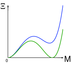
Figure 6: (color online) Schematic behavior of the thermodynamic potential $\Xi$ as a function of magnetization $M$. Upper curve: the first-order phase transition has not been reached yet but the system exhibits a metamagnetic transition in finite field. Lower curve: the first-order phase transition occurs.

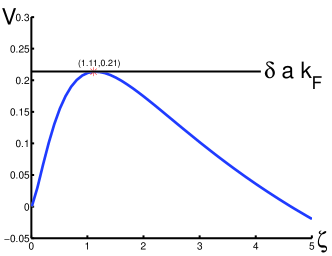
Figure 7: (color online) Function $V(\zeta)$ defined by Eq. (136). The first-order phase transition occurs when the maximum of $V$ reaches the value of $\delta\times(ak_{F})$.

At finite temperatures, the first-order transition occurs along the dashed line in Fig. 8, which starts at $\delta=\delta_{\text{cr}}$ at terminates at a tricritical point $(\delta_{\text{tc}},T=T_{\mathrm{tc}})$ (Ref. griffiths, ; belitz05, ). For $T>T_{\mathrm{tc}}$, the transition is second-order (solid line in Fig. 8). The tricritical temperature can be estimated from the condition that the $M^{4}/(\nu^{4}v^{2}_{F}T)$ term, which replaces the $|M|^{3}$ one at finite $T$, becomes comparable to the regular $bM^{4}$ term. In our model, $b\sim a/\nu^{4}v_{F}^{3}$. This gives $T_{\text{tc}}\sim v_{F}/a\sim{\tilde{\Delta}}_{\text{cr}}$. To find the numerical prefactor, one needs to evaluate the entire thermodynamic potential at finite $T$ but we are not going to dwell on it here.

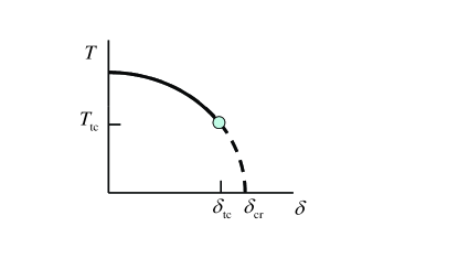
Figure 8: (color online) Phase diagram of a ferromagnetic phase transition. The lines of second- and first-order transitions (solid and dashed lines, respectively) are separated by a tricritical point.

III.5.2 Spiral magnetic phase

We now turn to another scenario of a phase transition, which is possible due to a nonanalytic behavior of the spin susceptibility as a function of the wavenumber. belitz ; chm03 ; pepin_prl ; pepin_prb Away from the QCP, $\chi(q)$ scales as $|q|$; near the QCP, the non-FL mass renormalization changes this scaling to $|q|^{3/2}$. As in the previous Section, it will turn out that for $ak_{F}\gg 1$, the instability occurs before the system enters into the $|q|^{3/2}$ regime. Therefore, we start with a FL form of $\chi(q)$ derived in Ref. pepin_prb, . In the long-range interaction model,

$$\chi^{-1}(q)\propto\delta+\left(aq\right)^{2}-\frac{4}{3\pi}\left(1+\lambda\right)\frac{|q|}{k_{F}}.$$ (142)

Equation (142) is valid for a moderate mass renormalization: $(1+\lambda)\ll 1/\sqrt{\delta}$. A spiral instability as $q=q_{\text{cr}}$ occurs when conditions $\chi^{-1}=0$ and $d\chi^{-1}/d|q|=0$ are satisfied simultaneously. This gives

$$q_{\text{cr}}=\frac{2}{3\pi}\frac{1+\lambda}{k_{F}a^{2}}$$ (143)

$$\delta^{\text{s}}_{\text{cr}}=\frac{4}{9\pi^{2}}\frac{(1+\lambda)^{2}}{k_{F}^{2}a^{2}}.$$ (144)

Since $\lambda$ depends on $\delta$ itself, as specified by Eq. (89), Eq. (144) represents an equation for $\delta^{\text{s}}_{\text{cr}}$. Solving this equation, we find that the spiral instability occurs at

$$\delta^{\text{s}}_{\text{cr}}=\left(\frac{1}{3\pi}+\sqrt{\frac{1}{\left(3\pi\right)^{2}}+\frac{1}{2\pi}}\right)\frac{1}{\left(ak_{F}\right)^{2}}\approx 0.52/\left(ak_{F}\right)^{2}.$$ (145)

At this $\delta$, $\lambda\sim 1$ and $(1+\lambda)^{2}\delta\sim\delta\ll 1$, so that Eq. (142) is, indeed, applicable.

Comparing the critical values of $\delta$ for the spiral instability and the first-order phase transition [cf. Eq. (141)], we see that

$$\delta_{\text{cr}}/\delta^{\text{s}}_{\text{cr}}\sim ak_{F}\gg 1.$$ (146)

This means that the first-order transition occurs before the spiral instability.

III.5.3 Re-entrant second-order phase transition

Another interesting consequence of the nonanalytic behavior of the susceptibility is a re-entrant second-order phase transition. This effect occurs due to a nonanalytic temperature dependence of $\chi$. Suppose that we are still far away from the tricritical point, so that the nonanalyticity of $\Xi$ as a function of $M$ does not play a role. Taking into account the regular $T$ dependence of $\chi$, which arises from energies of order of the bandwidth, we have from (122)

$$\chi^{-1}(T)=\chi_{0}\left[\delta+(T/T_{0})^{2}-(T/\epsilon_{F})\ln(|\delta|^{-1})\right],$$ (147)

where $T_{0}\sim W$. The critical temperature of the second-order transition is determined from the condition $\chi^{-1}(T_{c})=0$. In the absence of the nonanalytic term, the solution exists only for $\delta<0$ at $T_{c}=T_{0}\sqrt{-\delta}$ and the transition line $T_{c}(\delta)$ has a negative curvature for negative $\delta$. Due to the nonanalytic term, there exist two solutions of $\chi^{-1}(T_{c})=0$ for $\delta>0$ (see Fig. 9). One of them, $T_{c1}$, vanishes as $\delta/\ln\left(\delta^{-1}\right)$ at $\delta\to 0$, while the second behaves as $T_{c2}\sim\ln\left(\delta^{-1}\right)$. The two branches match at some (positive) value of $\delta=\delta_{R}$. As a result, the phase transition occurs at $\delta>0$, and the phase diagram exhibits a re-entrant behavior. Depending on whether the tricritical point is to the right or to the left of the reentrant point, the phase diagram has the forms shown in Fig. 9.

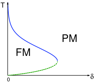
Figure 9: (color online) Re-entrant phase diagram of a second-order ferromagnetic phase transition. The two curves correspond to two solutions of Eq. (147).

III.6 Cooper channel near the quantum critical point

We now address the issue of Cooper renormalization near a ferromagnetic QCP. We recall that away from the QCP, the backscattering amplitude vanishes at $T\to 0$ as $1/\ln[\max\{T,{\tilde{\Delta}}\}]$ due to singular renormalizations in the Cooper channel. Consequently, the backscattering contribution to the spin susceptibility is reduced by a factor of $1/\ln^{2}[\max\{T,{\tilde{\Delta}}\}]$ as compared to non-backscattering contributions. The question is to what extent the Cooper renormalization affects the susceptibility near the QCP. This is an important issue because the sign of $\chi(T,H)$ determines whether the transition becomes first order or remain continuous. In the preceding discussion of the phase transition, we approximated the scattering amplitude by a single component $f_{s,0}$, which diverges at the QCP, and neglected all other components. This is certainly inconsistent with the vanishing of $f_{s}(\pi)$ at $T=0$, as it is the sum of all components that must vanish. We now include Cooper renormalization into consideration. For definiteness, we consider $\delta\chi(T,H=0)$.

First, we show that the logarithmical renormalization of $f_{s}(\pi)$ starts below some temperature which becomes progressively smaller as the system approaches the QCP and $|f_{s,0}|$ increases. To estimate this scale, we consider a vertex $\Gamma(k,p;p,k)$. When ${\bf k}$ and ${\bf p}$ are projected onto the Fermi surface and corresponding frequencies are set to zero, $\Gamma$ coincides with the scattering amplitude $f_{s}(\theta)$, which depends on the angle $\theta$ between ${\bf k}$ and ${\bf p}$. The backscattering amplitude corresponds to $\theta=\pi$.

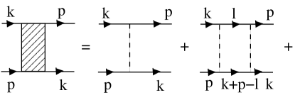
Figure 10: Renormalization of vertex $\Gamma(k,p;p,k)$ (hatched) in the Cooper channel. Dashed lines are irreducible Cooper amplitudes.

This vertex can be expressed as a series of diagrams in the Cooper channel (cf. Fig.10). The dashed lines are irreducible amplitudes $\gamma_{C}(\theta)$ which, in general, depend on the scattering angle, e.g., on the angle $\theta^{\prime}$ between ${\bf k}$ and ${\bf l}$ in second term of the series. Integrating over the magnitude of ${\bf l}$ and summing over the internal fermion frequencies, we obtain for the Cooper bubble

$$\Pi_{c}(\theta)\propto\frac{1}{\lambda}\ln\frac{1}{\cos\theta/2},$$ (148)

where, we remind, $\lambda\gg 1$ is the mass renormalization factor. As a result, the series for $f_{s}(\theta)$ reads

$$f_{s}(\theta)=\gamma_{C}(\theta)+\frac{\gamma^{(2)}_{C}(\theta)}{\lambda}\ln\frac{1}{\cos(\theta/2)}+\frac{\gamma^{(3)}_{C}(\theta)}{\lambda^{2}}\ln^{2}\frac{1}{\cos(\theta/2)}+\ldots$$ (149)

where $\gamma_{C}^{(j)}$ are the angular convolutions of two and more irreducible amplitudes; for example, $\gamma^{(2)}_{C}(\theta)=\int d\phi\gamma_{C}(\phi)\gamma_{C}(\theta-\phi)$, etc. Since irreducible amplitudes $\gamma_{C}(\theta)$ and $\gamma^{(j)}(\theta)$ are regular functions of $\theta$ near $\pi$, they can be replaced by constants $\gamma_{C}(\pi)$ and $\gamma^{(j)}(\pi)$ for $\theta\approx\pi$. Near $\theta=\pi$, $f_{s}(\theta)$ then becomes

$$f_{s}(\theta) \approx c_{1}+\frac{c_{2}}{\lambda}\ln\frac{1}{\cos(\theta/2)}+\frac{c_{3}}{\lambda^{2}}\ln^{2}\frac{1}{\cos(\theta/2)}+...$$ (150)

$$=f_{s,0}+\sum_{n>0}f_{s,n}\cos(n\theta).$$

The Cooper bubbles in Eq. (150) have regular expansions over angular harmonics; for example $\ln\left(\cos\theta/2\right)=-\ln 2+\sum_{n>0}(-)^{n+1}\cos(n\theta)/2n$, etc. Equating the prefactors of the $\cos(n\theta)$ terms in the first and second lines of Eq. (150), we obtain

$$f_{s,0} = c_{1}+\frac{c_{2}}{\lambda}\ln 2+\ldots$$

$$f_{s,n} = \frac{c_{2}}{\lambda}\frac{(-)^{n}}{2n}+\ldots$$ (151)

According to our assumption of a Pomeranchuk-like instability, $|f_{s,0}|\gg 1$ while $|f_{s,n>0}|\lesssim 1$. Therefore, $c_{1}=f_{s,0}+O(1)$. Dropping terms of order unity, the first line of Eq. (150) can be rewritten as

$$f_{s}(\theta)=f_{s,0}+\frac{c_{2}}{\lambda}\ln\frac{1}{\cos(\theta/2)}+\frac{c_{3}}{\lambda^{2}}\ln^{2}\frac{1}{\cos(\theta/2)}+\ldots$$ (152)

The angular-dependent terms in Eq. (152) are of order unity for $\theta\sim 1$. As $\theta$ approaches $\pi$, they increase and cancel the large, angular-independent term, $f_{s,0}$. This is how the vanishing of $f_{s}(\pi)$ happens. However, the cancellation occurs only for angles exponentially close to $\pi$: $\pi-\theta\sim\exp\left(-|f_{s,0}|\lambda/c_{1}\right).$ Associating typical $\pi-\phi$ with typical $T/\epsilon_{F}$, we conclude that the characteristic temperature, below which Coooper renormalization becomes crucial, is exponentially small in $|f_{s,0}|\lambda\sim(1+g_{s,0})^{-3/2}$.

These exponentially small temperatures are of no relevance for the preceding discussion, as they are lower that the temperature of the tricrical point, at which the second-order phase transition turns into a first-order one.

Still, the very fact that Cooper renormalizations bring about higher harmonics of $f_{s}(\phi)$, which scale as $\ln{\epsilon_{F}/T}$ requires some attention because the divergent harmonic of the scattering amplitude , $f_{s,0}$, enters $\delta\chi(T)$ only logarithmically [see Eq. (49], and the presence of extra $\ln T$ terms may affect the temperature dependence of $\chi$.

To address this issue, we use a simplified model, in which partial components of $f_{s}(\theta)$ with $n>0$ are absorbed into an effective temperature-dependent component $f_{s,1}$ modelled as

$$f_{s,1}=\frac{\frac{t}{\lambda}\ln{\frac{\epsilon_{F}}{T}}}{1+\frac{t}{\lambda|f_{s,0}|}\ln{\frac{\epsilon_{F}}{T}}},$$ (153)

where $t\sim 1$ is a constant. This interpolation formula reproduces correctly the limiting forms of $f_{s,1}$. Indeed, if $\ln\left(\epsilon_{F}/T\right)/\lambda|f_{s,0}|$ is small, $f_{s,1}$ scales as $(1/\lambda)\ln{\epsilon_{F}/T}$, consistent with the perturbation theory. If $\ln\left(\epsilon_{F}/T\right)/\lambda|f_{s,0}|$ is large, $f_{s,1}$ approaches $f_{s,0}$, consistent with the vanishing of $f_{s}(\pi)=f_{s,0}-f_{s,1}$ at $T=0$.

We now use Eqs. (50) and (51) for the susceptibility and compare the contributions from $f_{s,0}$ and $f_{s,1}$. Before substituting $f_{s,1}$ from Eq. (153) into Eq. (50) for the susceptibility, we need to account for the mass renormalization in the expressions for the functions $F_{1}(f_{s,0})$ and $F_{2}(f_{s,0})$, which amounts to replacing $f_{s,0}$ by $f_{s,0}/\lambda$ in the arguments of $F_{1}$ and $F_{2}$. Since $F_{1}(f_{s,0})$ scales as $\ln|f_{s,0}|$, it is not affected by mass renormalization. On the other hand, the asymptotic behavior of $F_{2}(f_{s,0})\approx 2f_{s,0}$ in the absence of mass renormalization must be replaced by $2f_{s,0}/\lambda$.

Using the modified expressions for $F_{1}$ and $F_{2}$ in Eq. (50) and the perturbative form $f_{c,1}\approx(c/\lambda)\ln{\epsilon_{F}/T}$, valid for all but exponentially small $T$, we find

$$\delta\chi(T,H=0)=\chi^{2D}_{0}\left(\frac{{\tilde{\mu}}_{B}}{\mu_{B}}\right)^{2}\frac{T}{{\tilde{\epsilon}}_{F}}\left[\ln{|f_{s,0}|}-\frac{4c}{\lambda^{2}}\ln{\frac{\epsilon_{F}}{T}}\right].$$ (154)

This is the key result. We see that Cooper renormalization generates a $\ln T$ correction to our earlier result for $\chi(T)$ in the isotropic scattering model. However, at all but exponentially small $T$ the correction is small in $1/\lambda^{2}$ and can be safely neglected. We conclude, therefore, that the sign and magnitude of $\chi(T,H=0)$ near the QCP is not affected by renormalizations in the Cooper channel.

The same consideration and conclusion hold also for $\chi(H,T=0)$.

IV Magnetic response in 3D

In this Section, we discuss the nonanalytic behavior of the spin susceptibility in 3D. The behavior of $\delta\chi(T,q,H=0)$ has been considered in Refs. bealmonod68, ; rasolt, ; pethick, ; belitz, ; chm03, ; chmm, ; betouras, ; dassarma, . As the Kohn anomaly is logarithmic in 3D, the corresponding nonanalyticities are also only logarithmic: $\delta\chi(T,q,H=0)\propto q^{2}\ln{\cal E}$, where ${\cal E}=\max\{v_{F}|q|,T\}$, and $\delta\chi(T=0,q=0,H)\propto H^{2}\ln|H|$. It was argued in Refs. belitz_rmp, ; belitz05, that these non-analyticities give rise to tricritical points, observed in 3D itinerant ferromagnets. belitz_rmp However, the relative weakness of nonanalytic terms in 3D raises a concern whether the tricritical behavior is indeed caused by the many-body physics or is due to some single-particle effects, such as features in the density of states schofield or magnetoelasticity larkin . In this Section, we show that logarithmic nonanalyticities are weakened even further by the mass renormalization in the vicinity of a 3D FM QCP, to $q^{2}\ln|\ln{\cal E}|$ and $H^{2}\ln|\ln|H||$ forms, respectively .

Another peculiarity of the 3D case is that the $T$-dependence of $\chi(T,H=0,q=0)$ is analytic: $\delta\chi(T)\propto c_{3D}T^{2}$ (Refs. bealmonod68, ; pethick, ). For a Galilean-invariant system (with a quadratic fermion dispersion), such as He³, the coefficient $c_{3D}$ was shown to be negative in Ref. bealmonod68, , i.e., the $T$-dependence of $\chi$ has the same sign as in a Fermi gas. We reanalyze this result in Sec. IV.0.2 and show that the magnitude and sign of $c_{3D}$ are nonuniversal, i.e., they depends on details of the fermion dispersion. This may explain while $c_{3D}$ is positive in He³ (Ref. He3chi, ) but negative in some exchange-enhanced paramagnets. co

IV.0.1 Magnetic-field dependence of the susceptibility

We first discuss the nonanalytic behavior of the susceptibility at $T=0$ in the perturbation theory.

Perturbation theory

To obtain the $H^{2}\ln|H|$ field dependence of the spin susceptibility in 3D at $T=0$, it suffices to expand the integral for $\Xi$ to order $H^{4}$ and verify that the prefactor diverges logarithmically. Cutting off the singularity at the scale set by $H$, one arrives at the $H^{4}\ln|H|$ behavior of $\Xi$ and, therefore, the $H^{2}\ln|H|$ behavior of $\delta\chi$.

At second order, $\Xi$ is still given by Eq. (7), where $\Pi_{\uparrow\downarrow}$ is now the 3D polarization bubble. For simplicity, we assume that the interaction is local, i.e., $U(q)=\mathrm{const}\equiv U$.

Similarly to the 2D case, $\Pi_{\uparrow\downarrow}$ can be separated into the static and dynamic parts as

$$\Pi_{\uparrow\downarrow}\left(\Omega_{m},q\right)=-\nu\left(1-\frac{i\Omega_{m}}{2v_{F}q}\ln\frac{i\Omega_{m}+v_{F}q+\Delta}{i\Omega_{m}-v_{F}q+\Delta}\right).$$ (155)

Here and till the end of this Section $\nu=mk_{F}/2\pi^{2}$ is density of states at the Fermi energy in 3D. Expanding the square of $\Pi_{\uparrow\downarrow}$ to order $\Delta^{4}$, we obtain

$$\Pi_{\uparrow\downarrow}^{2}\left(\Omega_{m},q\right)=\ldots+\nu^{2}\left(\frac{\Delta}{v_{F}q}\right)^{4}Q^{(2)}\left(\frac{\Omega_{m}}{v_{F}q}\right)+\ldots$$ (156)

where dots stand for $\Delta$-independent and regular $\Delta^{2}$ terms, and

$$Q^{(2)}\left(x\right)=x^{2}\frac{2\arctan(x^{-1})x\left[x^{2}-1\right]+x^{2}+4/3}{(x^{2}+1)^{4}}.$$ (157)

Substituting Eq. (156) into Eq. (7) and integrating over $\Omega_{m}$, we find that the $q$-integral is indeed logarithmic. Cutting off the logarithmic singularity by the field, we obtain

$$\Xi_{2}(T=0,H) = -\frac{u^{2}{\tilde{\Delta}}^{4}}{(2\pi)^{3}v_{F}{}^{3}}\int_{|{\tilde{\Delta}}|/{\tilde{v}}_{F}}^{k_{F}}\frac{dq}{q}\int_{-\infty}^{\infty}dy\text{ }Q\left(y\right)$$ (158)

$$= -\frac{u^{2}}{48\pi^{2}}\frac{{\tilde{\Delta}}^{4}}{v_{F}^{3}}\ln\frac{\epsilon_{F}}{\left|{\tilde{\Delta}}\right|},$$

where $u=U\nu$ and we used that $\int_{-\infty}^{\infty}dxQ^{(2)}\left(x\right)=\pi/6$. Consequently,

$$\delta\chi^{\left(2\right)}=u^{2}\frac{\Delta^{2}}{4\epsilon_{F}^{2}}\ln\frac{\epsilon_{F}}{\left|{\tilde{\Delta}}\right|}\chi_{0}^{3D},$$ (159)

where $\chi_{0}^{3D}=mk_{F}\mu_{B}^{2}/\pi^{2}$ is the spin susceptibility of a 3D Fermi gas. We see that that the sign of the field-dependence of the second-order contribution is metamagnetic, i.e., $\chi$ increases with $H$. This conclusion contradicts to Ref. bealmonodH, , where $\chi$ was found to decrease with $H$ as $H^{2}$ (without a logarithmic factor). Notice also that typical $\Omega_{m}$ and $q$ in Eq. (158) are such that $\Omega_{m}\sim{\tilde{v}}_{F}q\gg\Delta$. Therefore, even the second-order contribution in 3D does not arise entirely from backscattering processes.

Higher-order terms modify the second-order result by renormalizing static vertices in the skeleton diagram with two dynamical bubbles, and add new processes involving larger number of dynamic bubbles. For example, the nonanalytic part of diagram $e$ in Fig. 2 contains the cube of the dynamic bubble. Expanding $\Pi^{3}_{\uparrow\downarrow}$ to order $\Delta^{4}$, we obtain

$$\Pi_{\uparrow\downarrow}^{3}\left(\Omega_{m},q\right)=\ldots+\text{ }\nu^{2}\left(\frac{{\tilde{\Delta}}}{v_{F}q}\right)^{4}Q^{(3)}\left(\frac{\Omega_{m}}{v_{F}q}\right)+\ldots$$ (160)

where

$$Q^{(3)}\left(x\right)=x^{2}\frac{3x^{2}\left(x^{2}+1\right)\arctan^{2}(x^{-1})+x\left(4+3x^{2}\right)\arctan(x^{-1})-3x^{2}-1}{(x^{2}+1)^{4}}.$$ (161)

Substituting this expansion into Eq. (33), and performing the integrations over $\Omega_{m}$ and $q$ in the same way as in Eq. (158), we obtain

$$\delta\chi^{\left(3e\right)}=-\frac{\pi^{2}-8}{8}u^{3}\frac{{\tilde{\Delta}}^{2}}{4\epsilon_{F}^{2}}\ln\frac{\epsilon_{F}}{\left|{\tilde{\Delta}}\right|}\chi_{0}^{3D},$$ (162)

where we used that $\int_{-\infty}^{\infty}dxZ\left(x\right)=\pi(\pi^{2}-8)/16$. As it also the case in 2D, the signs of the second- and third-order contributions are opposite.

Quantum-critical behavior in 3D

The vicinity of a ferromagnetic QCP in 3D can be analyzed within the Eliashberg theory, in the same way it was done in Sec. III for the 2D case. Since our goal here is to obtain only the qualitative behavior of $\chi$, we will not repeat the manipulations within the spin-fermion model but just consider the RPA for $\Xi$, which reproduces correctly both the weak-coupling and quantum-critical limits. Summing up the RPA-series and replacing $u$ by $-g_{s,0}$ we obtain

$$\Xi(T=0,H)=\frac{1}{4\pi^{3}}\int_{-\infty}^{\infty}d\Omega_{m}\int_{0}^{\infty}q^{2}dq\ln\left[\delta+\frac{i\Omega_{m}}{2v_{F}q}\ln\frac{i\Omega_{m}+v_{F}q+{\tilde{\Delta}}}{i\Omega_{m}-v_{F}q+{\tilde{\Delta}}}\right]+\ldots$$ (163)

where $\Gamma=-g_{s,0}/(1+g_{s,0})$ and dots stand for regular terms. Expanding the integrand to fourth order in ${\tilde{\Delta}}$, and integrating over $\Omega_{m}$ and $q$, we obtain

$$\Xi(T=0,H)=-\frac{1}{2\pi^{3}}\frac{{\tilde{\Delta}}^{4}}{v_{F}^{3}}Z(\Gamma)\ln\frac{\epsilon_{F}}{\left|{\tilde{\Delta}}\right|},$$ (164)

where

$$Z(\Gamma)=\int_{0}^{\pi/2}d\phi\sin^{2}\phi\cos^{2}\phi\left[\frac{\cos 2\phi}{S}+\frac{11\cos^{2}\phi-2}{6S^{2}}+\frac{\cos^{2}\phi}{S^{3}}+\frac{cos^{2}\phi}{4S^{4}}\right]$$ (165)

and $S=\Gamma^{-1}-\phi\cot\phi$. For small $\Gamma$, $Z(\Gamma)\approx\pi\Gamma^{2}/24$, and Eq. (164) reduces to Eq. (158). At the QCP, $\Gamma\rightarrow\infty$, and $K(\Gamma)\approx 0.032$. Substituting this into (164) and differentiating twice over $H$, we obtain at the QCP

$$\delta\chi\approx 0.24\frac{{\tilde{\Delta}}^{2}}{4\epsilon_{F}^{2}}\ln\frac{\epsilon_{F}}{\left|{\tilde{\Delta}}\right|}\chi_{0}^{3D}.$$ (166)

Equation (166) is, however, incomplete as the RPA neglects mass renormalization which becomes singular near the QCP. Near a 3D QCP, the fermion self-energy behaves as $\Sigma(\omega_{m})\propto\omega_{m}|\ln\omega_{m}|$, i.e., at small frequencies it is parametrically larger than a bare $\omega_{m}$ term in the fermion propagator. Reevaluating the polarization bubble for dressed fermions, we obtain the same expression as in Eq. (155), except for $\Omega_{m}$ under the logarithm is replaced by $\Omega_{m}\ln{|\Omega_{m}|}$. Substituting this into Eq. (163), setting $\Gamma=\infty$, expanding again to order ${\tilde{\Delta}}^{4}$ and integrating first over $\Omega_{m}$ and then over $q$, we obtain

$$\Xi_{2}(T=0,H)\sim{\tilde{\Delta}}^{4}\int_{|{\tilde{\Delta}}|/{\tilde{v}}_{F}}^{k_{F}}\frac{dq}{q\ln q}\sim{\tilde{\Delta}}^{4}\ln|\ln|{\tilde{\Delta}}||.$$ (167)

Consequently,

$$\delta\chi\sim\chi_{0}^{3D}{{\tilde{\Delta}}^{2}}{\epsilon_{F}^{2}}\ln\ln\frac{\epsilon_{F}}{\left|{\tilde{\Delta}}\right|}.$$ (168)

This is a very weak nonanalytic dependence.

IV.0.2 Temperature dependence of the spin susceptibility

The temperature dependence of the spin susceptibility in 3D, $\delta\chi(T)\propto T^{2}$, was found perturbatively in Refs. pethick, ; chm03, and in the paramagnon model by Beal-Monod et al. (Ref.bealmonod68, ). Here, we consider the temperature dependence of the spin susceptibility of a 3D FL near a ferromagnetic QCP. As in Ref. bealmonod68, , we consider fermions with local interaction $U$ near a ferromagnetic QCP, so that $U\nu=-g_{s,0}\approx 1$. However, in contrast with Ref. bealmonod68, , we assume an isotropic but otherwise arbitrary energy spectrum $\varepsilon_{k}$. Correspondingly, the density of states, $\nu\left(\varepsilon_{k}\right)$, is an arbitrary function of the energy. As it will be shown in this Section, this generalization leads to a possibility of reversing the sign of the $T$-dependence of $\chi$.

Figure 11: Diagrams for the thermodynamic potential that give rise to the temperature dependence of the spin susceptibility in 3D. Top row: ladder diagrams; bottom row: ring diagrams.

The thermodynamic potential is given by Eq. (65); however, in contrast to the 2D case, the $T$-dependent part of the susceptibility comes not only from the ladder but also from the ring diagrams for $\Xi$. Consequently, the $\delta\Xi(T)$ term in Eq. (65) contains both types of diagrams (cf. Fig. 11): $\delta\Xi=\delta\Xi_{L}+\delta\Xi_{R}$, where

$$\delta\Xi_{L} = T\sum_{q}\left[\ln\left(1+U\Pi_{\uparrow\downarrow}\right)\right]$$ (169a)

$$\delta\Xi_{R} = \frac{1}{2}T\sum_{q}\left[\ln\left(1-U^{2}\Pi_{\uparrow}\Pi_{\downarrow}\right)+U^{2}\Pi_{\uparrow}\Pi_{\downarrow}\right],$$ (169b)

and

$$\Pi_{\uparrow,\downarrow}(\Omega_{m},q)=T\sum_{k}G_{\uparrow,\downarrow}(k+q)G_{\uparrow,\downarrow}(k)$$ (170)

is the polarization bubble composed of fermions with the same spin. The second-order diagram can be considered as a part of either the ladder or the ring series; we associate it with the ladder series and subtract the second-order term from the ring sequence.

The details of the calculation are presented in Appendix C. Here, we present the results for two different regimes near a QCP. The first one is the FL regime of small $T$ and finite $1+g_{s,0}$: $\left(1+g_{s,0}\right)^{3/2}\gg T/\epsilon_{F}$ . In this regime, $\delta\chi(T)$ scales as $T^{2}$, and the prefactor is the sum of the universal ($u$) and nonuniversal ($n$) contributions:

$$\chi^{-1}(T)=(\chi(0))^{-1}\left[1+\left(A_{u}+A_{n}\right)\left(\frac{T}{\epsilon_{F}}\right)^{2}\right],$$ (171)

where $\chi(0)=2\mu_{B}^{2}\nu/\left(1+g_{s,0}\right)$. The universal contribution has the same origin as in 2D: it arises due to a long-range dynamic interaction between fermions mediated by particle-hole pairs. The prefactor of this contribution, $A_{u}$, is given by

$$A_{u}=-\frac{1}{3}~{}\frac{1}{\left(1+g_{s,0}\right)^{2}}.$$ (172)

The nonuniversal part comes from the regular terms in the expansion of the polarization bubble in the momentum and frequency. The magnitude and the sign of the nonuniversal part depend on details of the fermion dispersion:

$$A_{n}=\frac{\pi^{2}}{4}\frac{\left(\nu^{\prime}\right)^{2}-(5/3)\nu\nu^{\prime\prime}}{\alpha\nu^{2}}\frac{\epsilon_{F}^{2}}{\left(1+g_{s,0}\right)^{2}},$$ (173)

where $v_{k}=d\varepsilon_{k}/dk$, $m_{k}^{-1}=d^{2}\varepsilon_{k}/dk^{2}$, $\nu^{\prime}=d\nu(\varepsilon_{k})/d\varepsilon_{k}|_{\varepsilon_{k}=\epsilon_{F}}$, $\nu^{\prime\prime}=d^{2}\nu(\varepsilon_{k})/d\varepsilon_{k}^{2}|_{\varepsilon_{k}=\epsilon_{F}}$. The coefficient $\alpha$ determines the $q$ dependence of the static bubble for free fermions in 3D

$$\Pi(\Omega_{m}=0,q)=-\nu\left[1-\frac{\alpha}{12}\left(\frac{q}{k_{F}}\right)^{2}\right]$$ (174)

and is given by

$$\alpha=\frac{k_{F}^{2}}{\nu}\frac{d}{d\varepsilon_{k}}\left\{\nu\left[2\frac{v_{k}}{k}+\frac{1}{m_{k}}\right]-\frac{2}{3}\frac{d}{d\varepsilon_{k}}\left[\nu v_{k}^{2}\right]\right\}\Big{|}_{\varepsilon_{k}=\epsilon_{F}}.$$ (175)

For a power-law dispersion, $\varepsilon_{k}=Ak^{\gamma}$, we have $\alpha=(\gamma+1)/3$. For a quadratic dispersion, $\gamma=2,\alpha=1$ and

$$A_{n}=\frac{\pi^{2}}{6}\frac{1}{(1+g_{s,0})^{2}}.$$ (176)

Comparing (172) and (176), we see that $A_{n}$ is positive and larger in magnitude than $A_{u}$: $A_{u}/A_{n}=-\pi^{2}/2\approx-4.93$. This is the result found in Ref. bealmonod68, . In this case, $\chi$ decreases with $T$:

$$\chi(T)=\frac{\chi(0)}{1+g_{s,0}+\frac{\pi^{2}-2}{6}\frac{1}{1+g_{s,0}}\left(\frac{T}{\epsilon_{F}}\right)^{2}}$$ (177)

This case is perhaps most relevant for He³. However, for more complex dispersions (relevant for anisotropic FLs in metals), the universal term can win over the nonuniversal one. Indeed, because $\alpha$ must be positive regardless of the dispersion (otherwise, a system of free fermions on a lattice would have a magnetic instability at finite $q$), the sign of $A_{n}$ is determined by the the sign of the combination $(\nu^{\prime})^{2}-(5/3)\nu\nu^{\prime\prime}$, entering Eq. (173). We see that $A_{n}>0$ as long as $\nu^{\prime\prime}<0$. On the other hand, if the Fermi energy is near the minimum in the density of states, where $\nu^{\prime}=0$ and $\nu^{\prime\prime}>0$, then $A_{n}<0$ and $\chi$ increases with $T$. Therefore, both types of the $T$-dependences are possible in metals. An increase of $\chi(T)$ with $T$ was observed in a number of strongly paramagnetic metals co .

Next, we consider the quantum critical regime: $T/\epsilon_{F}\gg\left(1+g_{s,0}\right)^{3/2}$. Here both universal and non-universal terms scale as $T^{4/3}$ (Ref. 3/4, ). A detailed calculation shows that

$$\chi^{-1}(T)=\left(2\mu_{B}^{2}\nu\right)^{-1}b\left(B_{u}+B_{n}\right)\left(T/\epsilon_{F}\right)^{4/3}$$ (178)

where $B_{u}=-8/\pi^{2}$ is the universal, low-energy contribution, $B_{n}$ is the nonuniversal contribution whose form depends on the details of the fermion dispersion, and $b=2^{2/3}(6\pi)^{1/3}\Gamma(4/3)\zeta(4/3)/3^{5/2}\approx 0.871$, with $\Gamma(x)$ and $\zeta(x)$ being the $\Gamma$- and $\zeta$-functions, respectively. For the quadratic dispersion, $B_{n}=1>8/\pi^{2}$ and the susceptibility is positive, i.e., the system is stable. It is possible, however, that $B$ is smaller than $8\pi^{2}$ for a more complex dispersion, in which case the susceptibility is negative at the QCP. This implies that the transition line $T_{c}(g_{s,0})$ may have “wrong” sign of the slope at small $T$, as in Fig. 9, and the system exhibits a reentrant ferromagnetic transition before reaching the QCP at $T=0$.

There is also a more fundamental reason for the re-entrant behavior. In the calculation that led us to Eq. (178), we neglected the fermion self-energy, which scales as $\omega_{m}\ln\omega_{m}$ at the QCP. Including the self-energy, we find that the universal, negative contribution to the inverse susceptibility [the $-8/\pi^{2}$ term in Eq. (178)] acquires an extra factor of $(\ln T)^{2}$, while the non-universal contribution remains the same. As a result, the universal term wins at low enough $T$, and the system displays a re-entrant behavior even for the quadratic dispersion.

V Conclusions

In this paper, we have considered nonanalytic spin response of an interacting Fermi system, both away from and near a ferromagnetic quantum critical point. Our two primary goals were i) to establish the sign of the magnetic-field and temperature dependences of the spin susceptibility in the Fermi-liquid regime and ii) analyze the stability of the continuous ferromagnetic quantum critical point in 2D. We found that higher-order processes, involving more than one particle-hole pair, may reverse the anomalous (positive) sign of the single particle-hole pair contribution in a 2D Fermi liquid. A controllable calculation within a large-$N$ model shows that this effect is more important than Cooper renormalizations of the backscattering amplitude considered in Refs. finn, ; finn_new, . For a 3D Fermi liquid, we showed that the sign of the $T$-dependence of $\chi$ is determined by the balance between universal and non-universal contributions; while the former depends only on the density of states and Fermi velocity near the Fermi level, the latter is sensitive to the actual form of the fermion spectrum away from the Fermi energy. We found that whereas the sign of $T$ and $H$ dependences of $\chi$ in the Fermi liquid regime depends on the detailed form of the interaction, the anomalous (positive) sign of these dependences is restored near a ferromagnetic quantum critical point. At the same time, the role of Cooper renormalizations is diminished even further near criticality. Analyzing different mechanisms for a breakdown of second-order phase transition, we showed, within the model of a long-range exchange interaction, that the first-order phase transition preempts an instability towards a spiral magnetic phase.

Appendix A Spin susceptibility of a 2D Coulomb system in the large $N$ limit

In this Appendix, we calculate the nonanalytic magnetic-field dependence of the spin susceptibility for a valley-degenerate 2D electron gas with Coulomb interaction. We assume that there are $N_{v}$ degenerate orbital valleys, so that the total (spin$\times$valley) degeneracy is $N=2N_{v}\gg 1$. For simplicity, we consider only the $T=0$ case.

Ring diagrams

Since each polarization bubble comes with a large factor of $N$, the leading contribution to the thermodynamic potential is given by a series of ring diagrams [diagrams a,b… in Fig. 2], which contain a maximum number of bubbles at each order. The sum of ring diagrams gives

$$\Xi_{N=\infty}=\frac{1}{2}T\sum_{q}\ln\left[1-\frac{N}{2}U\left(q\right)\left(\Pi_{\uparrow}+\Pi_{\downarrow}\right)\right],$$ (179)

where $U(q)=2\pi e^{2}/q$ is the bare Coulomb potential. The nonanalytic dependence of $\Xi$ is determined by $q$ near $2k_{F}$. For $q\approx 2k_{F}$, the second term under the logarithm in Eq. (179) is of order $N(e^{2}/k_{F})m\sim g_{N}$, where $g_{N}$ is the dimensionless coupling constant defined in Eq. (61). For $g_{N}\ll 1$, one can expand the logarithm to second order in $U(q)$. This reproduces a weak-coupling result of Ref. betouras, . In the opposite limit of $g_{N}\gg 1$ (strong coupling), the second term under the logarithm dominates, and the field-dependent part of $\Xi_{N=\infty}$ reduces to

$$\Xi_{N=\infty}=\frac{1}{2}T\sum_{q}\ln\left[1-\left(P_{\uparrow}+P_{\downarrow}\right)/2\right],$$ (180)

where $P_{\uparrow,\downarrow}$ are the dynamic parts of the bubbles with the same spins, defined as

$$\Pi_{\uparrow,\downarrow}(\Omega_{m},q)=-\frac{m}{2\pi}\left(1-P_{\uparrow,\downarrow}\right).$$ (181)

To evaluate $\Xi_{N=\infty}$, we expand the logarithm in Eq. (180) in Taylor series

$$\Xi_{N=\infty}=-\frac{1}{2}T\sum_{q}\left[\frac{1}{2}\left(P_{\uparrow}+P_{\downarrow}\right)+\frac{1}{2}\left[\frac{1}{2}\left(P_{\uparrow}+P_{\downarrow}\right)\right]^{2}+\frac{1}{3}\left[\frac{1}{2}\left(P_{\uparrow}+P_{\downarrow}\right)\right]^{3}+\frac{1}{4}\left[\frac{1}{2}\left(P_{\uparrow}+P_{\downarrow}\right)\right]^{4}+\ldots\right].$$ (182)

This expansion can be viewed as a series of fictitious ring diagrams with each bubble being either $P_{\uparrow}$ or $P_{\downarrow}$ and the effective interaction being equal to unity.

At $T,H=0$ and $q\approx 2k_{F}$,

$$P_{\uparrow}=P_{\downarrow}=\left(\frac{{\bar{q}}}{2k_{F}}+\sqrt{\left(\frac{{\bar{q}}}{2k_{F}}\right)^{2}+\left(\frac{\Omega_{m}}{4\epsilon_{F}}\right)^{2}}\right)^{1/2},$$ (183)

where ${\bar{q}}=q-2k_{F}$ and $|{\bar{q}}|\ll k_{F}$ (Ref. chm03, ). For $|\Omega_{m}|\ll|{\bar{q}}|{\tilde{v}}_{F}$, Eq. (183) reduces to

$$P_{\uparrow}=P_{\downarrow}=\left\{\begin{array}[]{cl}&\left({\bar{q}}/k_{F}\right)^{1/2};\;{\rm for}\;{\bar{q}}>0;\\ &\sqrt{2}|\Omega_{m}|/2{\tilde{v}}_{F}\left(k_{F}|{\bar{q}}|\right)^{1/2},\;{\rm for}\;{\bar{q}}<0.\end{array}\right.$$ (185)

One can easily verify that the field dependence of the $\Xi_{N=\infty}$ comes only from the products of $P_{\uparrow,\downarrow}$ with opposite spins. At second order, there is only one such a term: $P_{\uparrow}P_{\downarrow}$. The $q$-integral of $P_{\uparrow}P_{\downarrow}$ diverges logarithmically for ${\bar{q}}<0$. Finite magnetic field splits the Fermi momenta of spin-up and spin-down fermions. This, along with with finite $\Omega_{m}$, regularizes the integral:

$$\int d{\bar{q}}P{\uparrow}P_{\downarrow} \sim \Omega_{m}^{2}\int^{-\max\{|\Omega_{m}|,|\Delta|\}}_{-k_{F}}d{\bar{q}}/|{\bar{q}}|$$ (186)

$$=-\Omega_{m}^{2}\ln\max\{|\Omega_{m}|,|\Delta|\}.$$

This is the same logarithmic behavior that we have already encountered in the perturbation theory [cf. Eq.  (10)]–it leads to a $|\Delta|^{3}$ term in $\Xi$. At third order, the nonanalytic dependence on $\Delta$ comes from $P_{\uparrow}^{2}P_{\downarrow}$. The $q$ integral of $P_{\uparrow}^{2}P_{\downarrow}$ yields $|\Omega_{m}|^{3}\int d{\tilde{q}}/|{\tilde{q}}^{3/2}\sim|\Omega_{m}|^{5/2}$. This leads to a $|\Delta|^{7/2}$ nonanalyticity in $\Xi$, which is weaker than the $|\Delta|^{3}$ one. All higher order contributions produce either analytic terms or nonanalytic terms with higher powers of $\Delta$. Therefore, as long as only ring diagrams are considered, the only source of a $|\Delta|^{3}$ nonanalyticity is the second order term in (182). Hence,

$$\Xi_{N=\infty}=-\frac{1}{8}T\sum_{q}P_{\uparrow}P_{\downarrow}.$$ (187)

This situation is to be contrasted with the regular perturbation theory [cf. Sec. II.1], where ring diagrams are built from the full bubbles $\Pi_{\uparrow,\downarrow}$ (see 181). There, diagrams to all orders yield $|\Delta|^{3}$ terms. For example, at third order one generates a $|\Delta|^{3}$ term by keeping $P_{\uparrow,\downarrow}$ parts in two out of three bubbles and replacing the third one by its constant part ($-m/2\pi$). A strong-coupling expansion that we consider here involves ring diagrams built from $P_{\uparrow,\downarrow}$ instead of the full bubbles. Since $P_{\uparrow,\downarrow}$ do not contain constant terms, diagrams containing more than two $P_{\uparrow,\downarrow}$ do not give rise to a $|\Delta|^{3}$ nonanalyticity.

An explicit computation of $\Xi_{N=\infty}$ from Eq. (187) is quite involved, because one needs to know the expressions for $2k_{F}$ bubbles in a finite field. Fortunately, there is no need to perform such a computation because the nonanalytic part of the second-order diagram for a short-range interaction

$$\Xi_{2} = -\frac{1}{2}U^{2}T\sum_{q}\Pi_{\uparrow}\Pi_{\downarrow}$$ (188)

contains the same combination of $P_{\uparrow}P_{\downarrow}$ as Eq. (187). Therefore,

$$\Xi_{N=\infty}=\frac{1}{4}\Xi_{2}|_{u=1},$$ (189)

where $u=\nu U$. Using Eq. (10) $\Xi_{2}$ and differentiating twice with respect to the field, we obtain

$$\delta\chi_{N=\infty}=\frac{|{\tilde{\Delta}}|}{8\epsilon_{F}}\chi^{2D}_{0}.$$ (190)

Notice that this result could be obtained from the second-order ring diagram by replacing the wavy line by the screened Coulomb potential for $N\to\infty$

$$\tilde{U}=\frac{2\pi e^{2}}{q+2\pi e^{2}\frac{m}{2\pi}N}\approx\frac{2\pi}{mN}.$$ (191)

The $2k_{F}$ ring diagrams can be viewed as series of backscattering events, hence Eq. (190) is the backscattering contribution to the susceptibility for a Coulomb interaction in the large-$N$ limit.

Cooper channel

Out of the subleading, $1/N$ diagrams that modify the backscattering contribution to $\delta\chi$, the most important ones are the Cooper diagrams which come with an additional logarithm, $L_{C}=\ln(W/|\Delta|)$. At low energies, when $L_{C}>N$, the Cooper diagrams become comparable to the ring ones.

To third order, a Cooper diagram is diagram c in Fig. 2 with wavy line replaced by the screened Coulomb interaction from Eq. (191). This diagram reads

$$\Xi_{C,3} = \frac{1}{3}\left(\frac{N}{2}\right)^{2}\tilde{U}^{3}T\sum_{q}\left(\Pi_{\uparrow\downarrow}^{C}\right)^{3},$$ (192)

where $\Pi_{\uparrow\downarrow}^{C}$ is a Cooper bubble composed of fermions with opposite spins

$$\Pi^{C}_{\uparrow\downarrow}=T\sum_{k}G_{\uparrow}(k+q)G_{\downarrow}(-k).$$ (193)

At $T=0$,

$$\Pi_{\uparrow\downarrow}^{C} = \frac{m}{2\pi}\text{Re}\ln\frac{W}{\Omega_{m}+i{\tilde{\Delta}}+\sqrt{(\Omega_{m}+i{\tilde{\Delta}})^{2}+\left(v_{F}q\right)^{2}}}$$ (194)

$$=\frac{m}{2\pi}\left[L_{C}+P^{C}_{\uparrow\downarrow}\right],$$

where $P^{C}_{\uparrow\downarrow}$ is a dimensionless function of two variables, $x=\Omega_{m}/|{\tilde{\Delta}}|$ and $y=\left(v_{F}q/{\tilde{\Delta}}\right)^{2}$:

$$P^{C}_{\uparrow\downarrow}=-\text{Re}\ln\left[x+i\text{sgn}{\tilde{\Delta}}+\sqrt{(x+i\text{sgn}{\tilde{\Delta}})^{2}+y}\right].$$ (195)

Substituting Eq. (194) into Eq. (192), we obtain

$$\Xi_{C,3} = \frac{T}{12N}\sum_{q}\Big{(}L_{C}^{3}+3L_{C}^{2}P^{C}_{\uparrow\downarrow}$$ (196)

$$+3L_{C}\left[P^{C}_{\uparrow\downarrow}\right]^{2}+\left[P^{C}_{\uparrow\downarrow}\right]^{3}\Big{)}.$$

Cooper renormalization of the backscattering amplitude comes from the third term in Eq. (196)

$$\Xi_{C,3}=\frac{1}{4N}L_{C}T\sum_{q}\left[P^{C}_{\uparrow\downarrow}\right]^{2},$$ (197)

while other terms either give field-independent contributions or generate $1/N$ corrections to the prefactor of the $\left|\Delta\right|^{3}$ term. We now recall that the second-order diagram (diagram a in Fig. 2) can be represented equivalently either in the particle-hole or the particle-particle form. The latter reads

$$\Xi_{2}=-\frac{1}{2}u^{2}T\sum_{q}\left[P^{C}_{\uparrow\downarrow}\right]^{2}.$$ (198)

Comparing Eqs. (197) and (198), we find that

$$\Xi_{C,3}=-\frac{L_{C}}{2N}\Xi_{2}|_{u=1}=-\frac{2L_{C}}{N}\Xi_{N=\infty}.$$ (199)

As a result,

$$\delta\chi_{C,3}=-\frac{2L_{C}}{N}\delta\chi_{N=\infty},$$ (200)

where $\delta\chi_{N=\infty}$ is given by Eq. (190).

Higher order Cooper diagrams (diagram d in Fig. 2 and similar diagrams at higher orders) form a ladder. At any order $n$, we need to select only the $L_{C}^{n-2}\left[P_{\uparrow\downarrow}^{c}\right]^{2}$ term from the $n^{\text{th}}$ power of the Cooper bubble. The $n^{\text{th}}$ order Cooper diagram gives

$$\Xi_{C,n} = \frac{\left(-\right)^{n-1}}{n}\left(\frac{N}{2}\right)\frac{n(n-1)}{2}^{2}L_{C}^{n-2}C_{2}^{n}\left(\frac{m\tilde{U}}{2\pi}\right)^{n}$$ (201)

$$\times T\sum_{q}\left[P^{c}_{\uparrow\downarrow}\right]^{2}.$$

Re-expressing again $T\sum_{q}\left[P^{C}_{\uparrow\downarrow}\right]^{2}$ via $\Xi_{2},$ we obtain for the $n^{\text{th}}$ order Cooper contribution to the susceptibility

$$\delta\chi_{C,n}=\left(-\right)^{n}(n-1)\left(\frac{L_{C}}{N}\right)^{n-2}\delta\chi_{N=\infty},\text{ for }n\geq 3.$$ (202)

Summing up all orders, we obtain

$$\delta\chi_{C}=\sum_{n=3}^{\infty}\delta\chi_{C,n}=\delta\chi^{N=\infty}\left(\frac{1}{(1+L_{C}/N)^{2}}-1\right).$$ (203)

Combining this result with Eq. (190), we find for the total backscattering contribution $\delta\chi_{\mathrm{BS}}=\delta\chi_{N=\infty}+\delta\chi_{C}$

$$\delta\chi_{\mathrm{BS}}=\frac{|\Delta|}{8\epsilon_{F}}\frac{\chi^{2D}_{0}}{\left(1+L_{C}/N\right)^{2}}.$$ (204)

$1/N$ corrections

The $1/N$ corrections to Eq. (204) come from diagrams of third and higher orders in the screened interaction (191), excluding the main logarithmic parts of Cooper diagrams. Some of these diagrams, e.g., diagrams b,d and f in Fig. 2, belong to backscattering type and contribute either non-logarithmic corrections to the backscattering amplitude or subleading logarithmic corrections in the Cooper channel. For example, fourth-order Cooper diagram d contains not only the $L^{2}_{C}$ term, already taken into account when summing up the leading logarithmic terms, but also a subleading, $L_{C}$, term. These diagrams change the two terms in the denominator of (204) as $1\to 1+O(1/N)$ and $L_{C}/N\to L_{C}(1/N+O(1/N^{2}))$. At low energies, i.e., for $L_{C}\gg N$, the entire backscattering contribution is then given by an asymptotic limit of Eq. (204):

$$\delta\chi_{\mathrm{BS}}=\frac{|\Delta|}{8\epsilon_{F}}\frac{\chi^{2D}_{0}N^{2}}{L_{C}^{2}}~{}\left(1+O\left(\frac{1}{N}\right)\right).$$ (205)

In addition, there are diagrams of different type, which do not participate in the renormalization of the backscattering amplitude. To leading order in $1/N$, this is diagram e in Fig. 2. This diagram has already been calculated in Sec. II.2.2: we just need to substitute $u=1/N$ into Eq. (36) and multiply the result by $(N/2)^{2}$. Combining this result with the backscattering contribution, we obtain the low-energy form of $\delta\chi$ in the large-$N$ model given by Eq. (62).

Appendix B Equivalence between the thermodynamic and Kubo-formula approaches for the susceptibility.

In this work, we were using a thermodynamic approach to spin susceptibility, in which one first evaluates the thermodynamic potential in finite magnetic field and then finds the susceptibility by differentiating the potential with respect to the field. Alternatively, one can find the susceptibility via the Kubo formula for the spin-spin correlation function. Certainly, the results of the two approaches must be equivalent in the linear-response regime. However, when going beyond the lowest-order linear-response diagrams, it is quite easy to miss certain diagrams which are generated automatically in the thermodynamic approach. Moreover, the diagrams for $\chi$ generated by differentiating the thermodynamic potential work even beyond the linear-response regime, i.e, for an arbitrary ratio of the temperature and the Zeeman energy (but for Zeeman energies still smaller than the Fermi one, when the magnetic-field dependence of the bare interaction can be neglected).

We now show how the diagrams for $\chi$ are generated within the RPA in the spin channel for a local bare interaction: $U(q)=\mathrm{const}=u/\nu$. In this case, the field-dependent part of the thermodynamic potential is given by Eqs. (65) and (66). The polarization operator is given by Eq. (4) with the Green’s functions from Eq. (14). Differentiating Eq. (66) and using the identities

$$\frac{\partial G_{\uparrow,\downarrow}}{\partial H}=\mp{\tilde{\mu}}_{B}G^{2}_{\uparrow,\downarrow}$$ (206)

we obtain

$$\delta\chi(T,H)=\delta\chi_{1}+\delta\chi_{2},$$ (207)

where

$$\delta\chi_{1}=2{\tilde{\mu}}_{B}^{2}T^{2}\sum_{q}\sum_{k}\frac{U}{1+U\Pi_{\uparrow\downarrow}(q)}\left[G^{2}_{\uparrow}(k)G^{2}_{\downarrow}(k+q)-G^{3}_{\uparrow}(k)G_{\downarrow}(k+q)-G_{\uparrow}(k)G^{3}_{\downarrow}(k+q)\right]$$

$$\delta\chi_{2}={\tilde{\mu}}_{B}^{2}T^{3}\sum_{q}\sum_{k_{1}}\sum_{k_{2}}\frac{U^{2}}{(1+U\Pi_{\uparrow\downarrow}(q))^{2}}\left[G^{2}_{\uparrow}(k_{1})G_{\downarrow}(k_{1}+q)-G_{\uparrow}(k_{1})G^{2}_{\downarrow}(k_{1}+q)\right]$$

$$\times\left[G^{2}_{\uparrow}(k_{2})G_{\downarrow}(k_{2}+q)-G_{\uparrow}(k_{2})G^{2}_{\downarrow}(k_{2}+q)\right].$$ (208)

Algebraic expressions for $\delta\chi_{1}$ and $\delta\chi_{2}$ are equivalent to diagrams in Fig. 12.

Figure 12: Diagrams for the spin susceptibility generated by differentiating the thermodynamic potential with respect to the magnetic field.

The first term in $\delta\chi_{1}$ is equivalent to diagram a for the vertex correction insertions into the bare particle-hole bubble; the second and third terms are equivalent to diagrams and b and c, which are self-energy corrections. The contribution $\delta\chi_{2}$ is equivalent to ”Aslamazov-Larkin” diagrams d and e, which contain two triads of fermion propagators, connected by the interaction lines. The wavy lines in these diagrams are spin propagators $1/(1+U\Pi_{\uparrow\downarrow}(q))$, while the vertices contain Pauli matrices ${\bf\sigma}_{\alpha\beta}$. The same diagrams have been used in Ref. pepin_prb, to analyze diagrammatically the momentum dependence of the spin susceptibility.

Appendix C Temperature dependence of the spin susceptibility in 3D

In this Appendix, we derive Eqs. (171-175), describing the temperature dependence of the spin susceptibility in a 3D FL near a ferromagnetic QCP.

As we said in the main text, the field-dependent part of the thermodynamic potential is represented by a sum of the ladder and ring diagrams, which contain polarization bubbles made of fermions both with the same and opposite spins: $\Pi_{\uparrow,\uparrow}$ ($\Pi_{\downarrow,\downarrow}$)) and $\Pi_{\uparrow\downarrow}$, respectively [cf. Eqs. (169a,169b)]. In 2D, the nonanalytic, $O(T)$ behavior of the spin susceptibility is associated with the field dependence of the the dynamic part of $\Pi_{\uparrow\downarrow}$. In 3D, the $T$ dependence of $\chi$ turns out to be analytic, and one needs to consider the field dependence of both static and dynamic parts of $\Pi_{\uparrow\downarrow}$, as well as the field dependence of $\Pi_{\uparrow}$ and $\Pi_{\downarrow}$ (cf. Eq. (170)).

We begin with $\Pi_{\uparrow\downarrow}$. Expanding $\Pi_{\uparrow\downarrow}(0,0)$ to order ${\tilde{\Delta}}^{2}$, we obtain

$$\Pi_{\uparrow\downarrow}\left(0,0\right)=\int\frac{d^{3}k}{\left(2\pi\right)^{3}}\int\frac{d\omega_{m}}{2\pi}G_{\uparrow}\left(\omega_{m},k\right)G_{\downarrow}\left(\omega_{m},k\right)=\frac{1}{{\tilde{\Delta}}}\int_{-{\tilde{\Delta}}/2<\varepsilon_{k}-\epsilon_{F}<{\tilde{\Delta}}/2}\frac{d^{3}k}{\left(2\pi\right)^{3}}=-\nu-\frac{\nu^{\prime\prime}{\tilde{\Delta}}^{2}}{24}.$$ (209)

We will also need a $q^{2}$ term in the expansion of a static bubble in zero magnetic field. To obtain this term for an arbitrary but isotropic dispersion, we expand the difference $\delta\Pi(q)=\Pi(\Omega=0,q)-\Pi(\Omega_{m}=0,q\to 0)$ to order $q^{2}$:

$$\delta\Pi(q)=\int\frac{d^{3}k}{\left(2\pi\right)^{3}}\left[\frac{f_{0}\left(\varepsilon_{\mathbf{k+q}}\right)-f\left(\varepsilon_{\mathbf{k}}\right)}{\varepsilon_{\mathbf{k+q}}-\varepsilon_{\mathbf{k}}}-f^{\prime}_{0}(\varepsilon_{\mathbf{k}})\right]=\int\frac{d^{3}k}{\left(2\pi\right)^{3}}\left[\frac{1}{2}f_{0}^{\prime\prime}\delta\varepsilon+\frac{1}{6}f_{0}^{\prime\prime\prime}\left(\delta\varepsilon\right)^{2}\right],$$ (210)

where $f_{0}(\varepsilon_{\bf k})$ is the Fermi function and

$$\delta\varepsilon=\varepsilon_{\mathbf{k+q}}-\varepsilon_{\mathbf{k}}.$$ (211)

For an isotropic system $\varepsilon_{\mathbf{k}}=\varepsilon_{k}$ and

$$\delta\varepsilon=\varepsilon\left(\sqrt{k^{2}+2\mathbf{k\cdot q+q}^{2}}\right)-\varepsilon_{k}=\varepsilon_{k}^{\prime}\left(qx+\frac{q^{2}}{2k}\right)+\frac{1}{2}q^{2}x^{2}\left(\varepsilon_{k}^{\prime\prime}-\varepsilon_{k}^{\prime}/k\right).$$ (212)

For the quadratic spectrum, the last term is equal to zero. Integrating by parts, we find

$$\int\frac{d^{3}k}{\left(2\pi\right)^{3}}f_{0}^{\prime\prime}\delta\varepsilon_{k} = \frac{q^{2}}{6}\frac{d}{d\varepsilon_{k}}\left[\nu\left(\varepsilon_{k}\right)\left(2\frac{\varepsilon_{k}^{\prime}}{k\left(\varepsilon_{k}\right)}+\varepsilon_{k}^{\prime\prime}\right)\right]\Big{|}_{\varepsilon_{k}=\epsilon_{F}}$$

$$\int\frac{d^{3}k}{\left(2\pi\right)^{3}}f_{0}^{\prime\prime\prime}\left(\delta\varepsilon_{k}\right)^{2} = -\frac{q^{2}}{3}\frac{d^{2}}{d\varepsilon_{k}^{2}}\left[\nu\left(\varepsilon_{k}\right)(\varepsilon_{k}^{\prime})^{2}\right]\Big{|}_{\varepsilon_{k}=\epsilon_{F}}.$$ (213)

Adding up these two results, we obtain

$$\Pi\left(0,q\right)=-\nu+\nu\alpha\frac{q^{2}}{12k_{F}^{2}},$$ (214)

where $\alpha$ is given by Eq. (175).

Combining Eqs. (209) and (214) with the dynamic part of $\Pi_{\uparrow\downarrow}$ from Eq. (155), we obtain a complete result for $\Pi_{\uparrow\downarrow}$:

$$\Pi_{\uparrow\downarrow}\left(\Omega_{m},q\right) = -\nu-\nu^{\prime\prime}\frac{{\tilde{\Delta}}^{2}}{24}+\nu\alpha\frac{q^{2}}{12k_{F}^{2}}$$ (215)

$$+\frac{i\nu\Omega_{m}}{2v_{F}q}\ln\frac{i\Omega_{m}+v_{F}q+{\tilde{\Delta}}}{i\Omega_{m}-v_{F}q+{\tilde{\Delta}}}.$$

Next, we consider $\Pi_{\uparrow}$ and $\Pi_{\downarrow}$, which depend on ${\tilde{\Delta}}$ only via the static parts

$$\Pi_{\uparrow,\downarrow}\left(0,0\right)=-\nu\left(\epsilon_{F}\pm{\tilde{\Delta}}/2\right)=-\left(\nu\pm\nu^{\prime}\frac{{\tilde{\Delta}}}{2}+\nu^{\prime\prime}\frac{{\tilde{\Delta}}^{2}}{8}\right).$$ (216)

Using Eq. (169a) for $\delta\Xi_{L}(T,H)$, we obtain

$$\delta\chi_{L}^{-1}=\frac{1}{\left(\mu_{B}\nu\right)^{2}}\frac{\partial^{2}\delta\Xi_{L}}{\partial{\tilde{\Delta}}^{2}}\Big{|}_{{\tilde{\Delta}}=0}=\frac{1}{\left(\mu_{B}\nu\right)^{2}}T\sum_{q}\left[\frac{U}{1+U\Pi_{\uparrow\downarrow}}\frac{\partial^{2}\Pi_{\uparrow\downarrow}}{\partial{\tilde{\Delta}}^{2}}-\frac{U^{2}}{\left(1+U\Pi_{\uparrow\downarrow}\right)^{2}}\left(\frac{\partial\Pi_{\uparrow\downarrow}}{\partial{\tilde{\Delta}}}\right)^{2}\right]\Bigg{|}_{{\tilde{\Delta}}=0}.$$ (217)

The derivatives of $\Pi_{\uparrow\downarrow}$ in Eq. (217) are found with the help of Eq. (215):

$$\frac{\partial^{2}\Pi_{\uparrow\downarrow}}{\partial{\tilde{\Delta}}^{2}}\Bigg{|}_{{\tilde{\Delta}}=0} = -\frac{\nu^{\prime\prime}}{12}+2\nu\frac{\Omega_{m}^{2}}{\left(\Omega_{m}^{2}+v_{F}^{2}q^{2}\right)^{2}}$$ (218a)

$$\left(\frac{\partial\Pi_{\uparrow\downarrow}}{\partial{\tilde{\Delta}}}\right)^{2}\Bigg{|}_{{\tilde{\Delta}}=0} = -\nu^{2}\frac{\Omega_{m}^{2}}{\left(\Omega_{m}^{2}+v_{F}^{2}q^{2}\right)^{2}}$$ (218b)

The first term in Eq. ( 217) gives a nonuniversal $T^{2}$ contribution, which can be obtained by expanding the prefactor $\left(1+U\Pi_{\uparrow\downarrow}\right)^{-1}$ to first order in $\Omega_{m}/v_{F}q$ and also expanding $\Pi_{\uparrow\downarrow}$ itself to order $\left(q/k_{F}\right)^{2}$. Doing so, we find

$$\left(\delta\chi_{L}^{(n)}\right)^{-1}=-\frac{1}{12\left(\mu_{B}\nu\right)^{2}}\frac{\nu^{\prime\prime}}{\nu}T\sum_{q}\left({1+g_{s,0}+\frac{\pi\left|\Omega_{m}\right|}{2v_{F}q}+\alpha\frac{q^{2}}{12k_{F}^{2}}}\right)^{-1}=-\frac{1}{12\chi(0)}\frac{k_{F}^{2}{\tilde{v}}_{F}^{2}}{\alpha}\frac{\nu^{\prime\prime}}{\nu}\frac{T^{2}}{\left(1+g_{s,0}\right)^{2}\nu{\tilde{v}}_{F}^{3}},$$ (219)

where $\chi(0)=2\mu_{B}^{2}\nu/\left(1+g_{s,0}\right)$. The Matsubara summation was performed using

$$T\sum_{\Omega_{m}}|\Omega_{m}|=\mathrm{const}-\frac{\pi}{3}T^{2}.$$ (220)

The second term in Eq.  (217) gives a contribution of order $T^{2}\ln{|1+g_{s,0}|}/(1+g_{s,0})$, which diverges weaker upon approaching the QCP than the $T^{2}/(1+g_{s,0})^{2}$ contribution in Eq. (219). Therefore, this contribution can be neglected.

The universal part of the ladder contribution comes from the second term of Eq. (217). We have

$$\left(\delta\chi_{L}^{\left(u\right)}\right)^{-1}=\frac{1}{\left(\mu_{B}\nu\right)^{2}}T\sum_{q}\frac{1}{\left(1+g_{s,0}+\frac{\pi\left|\Omega_{m}\right|}{2qv_{F}}\right)^{2}}\frac{\Omega_{m}^{2}}{\left(\Omega_{m}^{2}+v_{F}^{2}q^{2}\right)^{2}}=-\frac{2}{3\pi^{2}\chi(0)}\frac{T^{2}}{\left(1+g_{s,0}\right)^{2}\nu v_{F}^{3}}.$$ (221)

The total ladder contribution is the sum of Eqs. (219) and (221).

The contribution to $\chi$ from ring diagrams is obtained in the same way, and the result is

$$\delta\chi_{R}^{-1}=\frac{1}{2\left(\mu_{B}\nu\right)^{2}}T\sum_{q}\left\{-U^{2}\frac{\frac{\partial^{2}}{\partial{\tilde{\Delta}}^{2}}\left(\Pi_{\uparrow}\Pi_{\downarrow}\right)}{1-U^{2}\Pi_{\uparrow}\Pi_{\downarrow}}+U^{4}\frac{\left(\frac{\partial}{\partial{\tilde{\Delta}}}\left(\Pi_{\uparrow}\Pi_{\downarrow}\right)\right)^{2}}{\left(1-U^{2}\Pi_{\uparrow}\Pi_{\downarrow}\right)^{2}}\right\}\Big{|}_{{\tilde{\Delta}}=0}.$$ (222)

Using Eq. (216), we find that the second term in Eq. (222) vanishes, while the first one reduces to

$$\delta\chi_{R}^{-1}=\frac{1}{4(\mu_{B}\nu)^{2}}\left(\left(\nu^{\prime}\right)^{2}-\nu\nu^{\prime\prime}\right)T\sum_{\Omega_{m}}\int\frac{d^{3}q}{\left(2\pi\right)^{3}}\left[\frac{U^{2}}{1-U^{2}\Pi^{2}}\right],$$ (223)

where $\Pi$ is the polarization operator in the absence of the field. Obviously, the entire ring contribution is non-universal.

Near a ferromagnetic QCP, i.e, when $g_{s,0}\approx-1$, Eq. (223) can be simplified to

$$\delta\chi_{R}^{-1}=\frac{1}{4\mu_{B}^{2}\nu}\frac{\left(\nu^{\prime}\right)^{2}-\nu\nu^{\prime\prime}_{F}}{\nu^{2}}T\sum_{q}\left(1+g_{s,0}+\frac{\pi\left|\Omega_{m}\right|}{2v_{F}q}+\alpha\frac{q^{2}}{12k_{F}^{2}}\right)^{-1}=\frac{1}{8\chi(0)}\frac{k_{F}^{2}{\tilde{v}}_{F}^{2}}{\alpha}\frac{\left(\nu^{\prime}\right)^{2}-\nu\nu^{\prime\prime}}{\nu^{2}}\frac{T^{2}}{\left(1+g_{s,0}\right)^{2}\nu v_{F}^{3}}.$$ (224)

Combining $\delta\chi_{R}^{-1}$ with Eq. (219) for the nonuniversal part of the ladder contribution, we obtain Eq. (173), while the universal part of $\delta\chi_{L}^{-1}$ gives Eq. (172).

References

- (1) A. A. Abrikosov, L. P. Gorkov, and I. E. Dzyaloshinski, Methods of quantum field theory in statistical physics, (Dover Publications, New York, 1963); E. M. Lifshitz and L. P. Pitaevski, Statistical Physics, (Pergamon Press, 1980).
- (2) D. Belitz, T. R. Kirkpatrick, and T. Vojta, Rev. Mod. Phys. 77 579 (2005).
- (3) H. v. Löhneysen, A. Rosch, M. Vojta, and P. Wölfle, Rev. Mod. Phys. 79, 1015 (2007).
- (4) D. Coffey and K. S. Bedell, Phys. Rev. Lett. 71, 1043 (1993).
- (5) M. A. Baranov, M. Yu. Kagan, and M. S. Mar’enko, JETP Lett. 58, 709 (1993).
- (6) G. Y. Chitov and A. J. Millis, Phys. Rev. Lett. 86, 5337 (2001); ibid. Phys. Rev. B 64, 0544414 (2001).
- (7) A. V. Chubukov and D. L. Maslov, Phys. Rev. B 68, 155113 (2003); ibid. 69, 121102 (2004).
- (8) A. V. Chubukov, D. L. Maslov, S. Gangadharaiah, and L. I. Glazman, Phys. Rev. Lett. 95, 026402 (2005).
- (9) A. V. Chubukov, D. L. Maslov, S. Gangadharaiah, and L. I. Glazman, Phys. Rev. B 71, 205112 (2005).
- (10) V. M. Galitski, A. V. Chubukov, and S. Das Sarma, Phys. Rev. B 71, 201302 (2005).
- (11) J. Betouras, D. Efremov, and A. V. Chubukov, Phys. Rev. B 72, 115112 (2005).
- (12) G. Catelani and I. L. Aleiner, JETP 100, 331 (2005).
- (13) A. V. Chubukov, D. L. Maslov and A. J. Millis, Phys. Rev. B 73, 045128 (2006).
- (14) I. L. Aleiner and K. B. Efetov, Phys. Rev. B 74, 075102 (2006).
- (15) G. Schwiete and K. B. Efetov, Phys. Rev. B 74, 165108 (2006).
- (16) A. Shekhter and A. M. Finkelstein, Phys. Rev. B 74, 205122 (2006).
- (17) D. L. Maslov, A. V. Chubukov, and R. Saha, Phys. Rev. B 74, 220402 (2006).
- (18) A. Shekhter and A. M. Finkel’stein, Proc. Natl. Acad. Sci. U.S.A. 103, 15765 (2006).
- (19) D. Belitz, T. R. Kirkpatrick, and T. Vojta, Phys. Rev. B 55, 9452 (1997).
- (20) J. A. Hertz, Phys. Rev. B 14, 1165 (1976).
- (21) A. J. Millis, Phys. Rev. B 48, 7183 (1993).
- (22) T. Moriya, Spin Fluctuations in Itinerant Electron Magnetism (Springer, Berlin, 1985).
- (23) A. Casey, H. Patel, J. Nyeki, B.P. Cowan and J. Saunders, Pys. Rev. Lett. 90, 115301 (2003).
- (24) O. Prus, Y. Yaish, M. Reznikov, U. Sivan, and V. Pudalov Phys. Rev. B 67, 205407 (2003).
- (25) V. M. Pudalov, M. E. Gershenson, H. Kojima, in: Fundamental Problems of Mesoscopic Physics. Interaction and Decoherence, Eds. I. V. Lerner, B. L. Altshuler, and Y. Gefen, NATO Sci. Series, (Kluwer 2004), p. 309.
- (26) J. Zhu, H. L. Stormer, L. N. Pfeiffer, K. W. Baldwin, and K. W. West, Phys. Rev. Lett. 90, 056805 (2003).
- (27) T. Gokmen, M. Padmanabhan, E. Tutuc, M. Shayegan, S. De Palo, S. Moroni, and G. Senatore, Phys. Rev. B 76, 233301 (2007).
- (28) See, e.g., Guang-Ming Zhang, Yue-Hua Su, Zhong-Yi Lu, Zheng-Yu Weng, Dung-Hai Lee, Tao Xiang, arXiv:0809.3874 and references therein.
- (29) P. Simon and D. Loss, Phys. Rev. Lett. 98, 156401 (2007).
- (30) P. Simon, B. Braunecker, and D. Loss, Phys. Rev. B 77, 045108 (2008).
- (31) S. Chesi, R. A. Zak, P. Simon, and D. Loss, arXiv:0811.0996.
- (32) A. V. Chubukov and D. L. Maslov, Phys. Rev. B 76, 165111 (2007).
- (33) C.J. Pethick and G.M. Carneiro, Phys. Rev. A 7, 304 (1973); C. J. Pethick and G. M. Carneiro, Phys. Rev. B 11, 1106 (1975).
- (34) M. T. Béal-Monod, S.-K. Ma, and D. R. Fredkin, Phys. Rev. Lett. 20, 929 (1968).
- (35) G. M. Carneiro and C. J. Pethick, Phys. Rev. B 16, 1933 (1977).
- (36) K. Ikeda, K. A. Gschneidner, R. J. Stierman, T.-W. E. Tsang, and O. D. McMasters, Phys. Rev. B 29, 5039 (1984).
- (37) D. S. Greywall, Phys. Rev. B 27, 2747 (1983).
- (38) D. S. Greywall, Phys. Rev. B 41, 1842 (1990).
- (39) W. Kohn and J. Luttinger, Phys. Rev. Lett. 15, 524 (1965); D. Fay and J. Appel, Phys. Rev. B 20, 3705 (1979).
- (40) Y. Takada, Phys. Rev. B43, 5962 (1986).
- (41) S. V. Iordanskii and A. Kashuba, JETP Lett. 76, 563 (2002).
- (42) S. Gangadharaiah and D. L. Maslov, Phys. Rev. Lett. 95, 186801 (2005).
- (43) A. V. Chubukov, Phys. Rev. B 48, 1097 (1993)
- (44) We thank D. Loss for bringing this point to our attention.
- (45) J. M. Luttinger and J. C. Ward, Phys. Rev. 118, 1417 (1960).
- (46) A. V. Cubukov, Phys. Rev. B 71, 224431 (2005).
- (47) A. V. Chubukov, V. M. Galitski, and V. M. Yakovenko, Phys. Rev. Lett. 94, 046404 (2005).
- (48) B.L. Altshuler, L.B. Ioffe, and A. J. Millis, Phys. Rev. B 52, 5563 (1995).
- (49) J. Polchinski, Nucl. Phys. B 422, 617 (1994); V. Ogannesyan, S. A. Kivelson, and E. Fradkin, Phys. Rev. B 64, 195109 (2001); H. Y. Kee and Y.B. Kim, J. Phys: Condensed Matter 16, 3139 (2004); I. Vekhter and A. Chubukov, Phys. Rev. Lett. 93, 016405 (2004).
- (50) A. V. Chubukov, C. Pépin, and J. Rech, Phys. Rev. Lett. 92, 147003 (2004).
- (51) J. Rech, C. Pépin, and A. V. Chubukov, Rev. B 74, 195126 (2006).
- (52) A. V. Chubukov and D. L. Maslov, unpublished.
- (53) M. Dzero and L. P. Gor’kov, Phys. Rev. B69, 092501 (2004).
- (54) L. Dell Anna and W. Metzner, Phys. Rev. B 73, 045127 (2006); Phys. Rev. Lett. 98, 136402 (2007).
- (55) Ar. Abanov. A. V. Chubukov, J. Schmalian, Adv. Phys. 52, 119 (2003).
- (56) A. V. Chubukov, Phys. Rev. B 72, 085113 (2005).
- (57) G. M. Eliashberg, Sov. Phys. JETP 11, 696 (1960); ibid. 16, 780 (1963).
- (58) J. Bardeen and M. Stephen, Phys. Rev. 136, A1485 (1964).
- (59) R. E. Prange and L. P. Kadanoff, Phys. Rev. 134, A566 (1964).
- (60) R. Haslinger and A. V. Chubukov, Phys. Rev. B 67, 140504 (2003); ibid. 68, 214508 (2003); A. Chubukov, A. Finkelstein, R. Haslinger and D. Morr, Phys. Rev. Lett. 90, 077002 (2003); P. Monthoux and G.G. Lonzarich, Phys. Rev. B 69, 064517 (2004).
- (61) The numerical prefactor in differs from the one obtained in we_short , because the thermodynamic potential was defined in a different way. It agrees with the one obtained recently bec in the analysis of in the ferromagnetically ordered phase.
- (62) D. Belitz, T. R. Kirkpatrick, and J. Rollbühler, Phys. Rev. Lett. 94 247205 (2005).
- (63) R. B. Griffiths, Phys. Rev. B 7, 545 (1973).
- (64) V. M. Galitski and S. Das Sarma, Phys. Rev. B 70, 035111 (2004).
- (65) D. J. Geldart and M. Rasolt, Phys. Rev. B 15, 1523 (1977); ibid. 22, 4079 (1980).
- (66) K. G. Sandeman, G. G. Lonzarich, and A. J. Schofield, Phys. Rev. Lett. 90, 167005 (2003).
- (67) A. I. Larkin and S. A. Pikin, JETP 29, 891 (1969).
- (68) G. G. Lonzarich, in Electron, edited by M. Springford (Cambridge University Press, Cambridge, England, 1997).
- (69) J. C. Wheatley, in Quantum Fluids, edited by A. F. Brewer (North-Holland Publishing Company, Amsterdam, The Netherlands, 1966); A. C. Anderson, W. Reese, and J. C. Wheatley, Phys. Rev. 127, 671 (1962).
- (70) M. T. Béal-Monod and E. Daniel, Phys. Rev. Lett. 68, 3817 (1992).
- (71) D. Efremov, D. Betouras, and A. Chubukov, Phys. Rev. B 77, 220401 (2008).