Toward constraints on galaxy formation scenarios: stellar properties from Galactic surveys

Abstract

We present some of the strategies being developed to classify and parameterize objects obtained with spectra from the Sloan Digital Sky Survey (SDSS) and the RAdial Velocity Experiment (RAVE) and present some results. We estimate stellar atmospheric parameters (effective temperature, gravity, and metallicity) from spectral and photometric data and use these to analyse Galactic populations. We demonstrate this through the selection of a sample of candidate Blue Horizontal-Branch and RR Lyrae stars selected from SDSS/SEGUE.

1 Introduction

The nature of the stellar populations of the Milky Way galaxy remains an important issue for astrophysics, because it addresses the question of galaxy formation and evolution and the origin of the chemical elements. To date, however, studies have been limited by the small number of stars that could be confidently identified as members of the various populations, and also by the lack of available spectroscopy from which radial velocities and estimates of atmospheric parameters (such as effective temperature, surface gravity, and metallicity) could be obtained.

With new ground-based and space-born survey missions currently under way or on the immediate horizon, such as SDSS, RAVE, LAMOST, and Gaia, we are in the golden age of Galactic astronomy. However, the classification of such a wide variety of objects coming available is a challenging one, which requires appropriate automated multi-dimensional data analysis techniques, and is a necessary step toward constraining scenarios of Galaxy formation.

2 Data

As training grounds and complements to Gaia, we here focus on the analysis of data coming available from two complementary on-going spectroscopic surveys.

The Sloan Digital Sky Survey

In the northern hemisphere, SDSS-I and its extension for Galactic studies, SDSS-II/SEGUE, have provided $9500$ square degrees of imaging data (position and multicolor photometry) for over $200$ million stars, taken with a dedicated 2.5-m telescope on Apache Point, New Mexico. Some $3500$ square degrees at lower Galactic latitudes ($|b|<40^{o}$) are included as well.

In addition to the imaging, these surveys obtained stellar spectra, covering the wavelength range $\lambda\lambda$ 3850–9000 $\AA$ at a resolving power $R\simeq 2000$, for approximately $300\,000$ Galactic stars in the magnitude range $14.0\leq g\leq 20.5$; the radial velocities have typical accuracy of $10\,{\rm km\,s^{-1}}$ (e.g., [Adelman-McCarthy et al. (2008), Adelman-McCarthy et al. 2008]; [Beers et al. (2004), Beers et al. 2004]).

The RAdial Velocity Experiment

In the southern hemisphere, using the 6dF multi-object spectrograph on the 1.2-m UK Schmidt Telescope of the Anglo-Australian Observatory, RAVE will measure radial velocities and stellar atmospheric parameters of up to one million bright stars by 2010. It has already observed over $250\,000$ stars away from the plane of the Milky Way ($|b|>25^{o}$) in the magnitude range $9<I<12$, obtaining medium-resolution spectra ($R\simeq 7500$) in the CaII triplet region ($\lambda\lambda$ 8410–8795 $\AA$).

In addition to cross-identification with photometric and astrometric catalogues, the second data release provides spectroscopic radial velocities with accuracy better than $2\,{\rm km\,s^{-1}}$ for about $50\,000$ stars, and stellar parameters for over $20\,000$ spectra ([Zwitter et al. (2008), Zwitter et al. 2008]).

3 Spectral Analysis and Classification

The main objectives of the classification are a discrete source classification which might account for the identification of new types of objects and the estimation of astrophysical parameters for specific classes. We use SDSS/SEGUE and RAVE spectra to develop, implement, and test several methods for this classification.

Principal Component Analysis

In terms of classification, a spectrum contains a large amount of redundant information. We investigate the application of principal components analysis (PCA) to the optimal compression of spectra.

Using a sample of synthetic spectra ([Munari et al. (2005), Munari et al. 2005]), we use PCA to form a set of linearly independent basis vectors with which to describe the data themselves, as well as any other newly observed spectrum. Figure 1 shows reduced spectral reconstructions (coloured lines) around the CaII triplet for three selected RAVE spectra (black lines), using different numbers of principal components computed from the synthetic spectra. The top and middle rows refer to the spectra of single stars with similar atmospheric parameters, as obtained previously and listed in the current catalogue, but with different of signal-to-noise ratios (namely, $SNR=49$ and $25$ respectively). The bottom row refers to the spectrum of a binary with high signal-to-noise ($SNR=55$).

From inspection of these reconstructions, one can see how the PCA approach – by keeping only the most significant few components – is able to retain essentially all of the useful information and, beside being able to recover missing and/or borderline features, acts as an effective filter to remove noise in the single star data set (see Fig. 1, top and middle rows). Furthermore, it is shown that this compression, which optimally removes noise, is able to isolate rare types of stars with strong features such as binaries (see Fig. 1, bottom row). As the template library only covers regular stars, peculiar objects (e.g., double-lined spectroscopic binaries and emission line objects) and outliers (e.g., new types of objects) are not represented correctly with a few principal components, which allows them to be efficiently detected. Thus, beside computational reasons (robustness and speed) and the higher accuracy achieved, this method can be used to identify/classify unusual spectra and discover natural classes among the data.

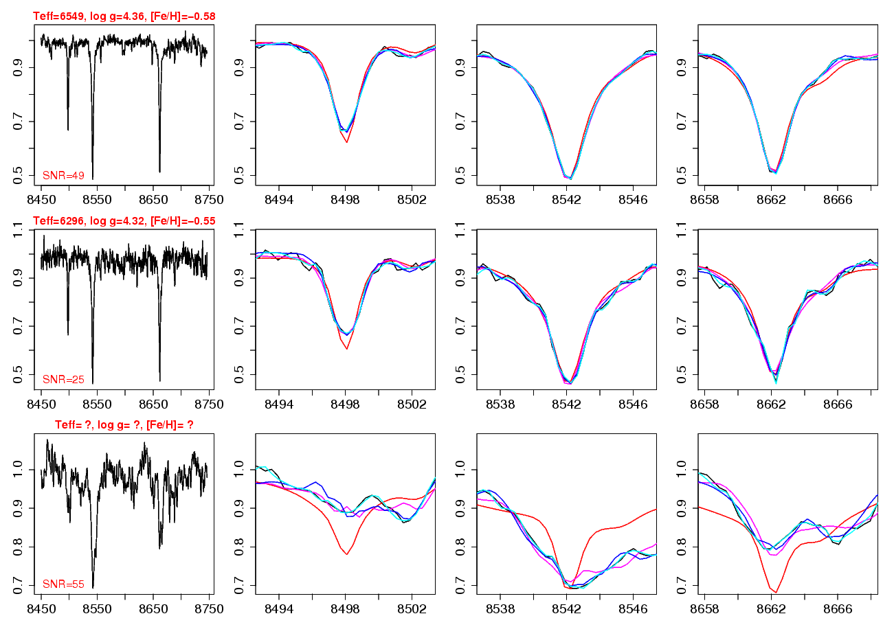
Figure 1: Reconstruction of RAVE spectra (black lines) by projection onto synthetic principal components. In each row, the spectrum on the left is the original and the following show, zooming in around the CaII triplet, its reconstructions using 5 (red), 50 (pink), 100 (blue), and 250 (cyan) principal components.

Discrete Source Classifier

In order to classify all sources (determining whether an object is a single star, binary, etc.), the DSC uses as its input spectra compressed via PCA (for speed and robustness of the classifier).

The algorithm is trained on synthetic spectra. Eight classes of astrophysical objects are considered. In addition to regular spectra from the stellar library by [Munari et al. (2005), Munari et al. (2005)], libraries for peculiar objects are built (Re Fiorentin et al. in preparation) and adopted. The former sample provides cool (T1: $T_{\rm eff}<5000$ K), medium-temperature (T2: $5000$ K $\leq T_{\rm eff}<10000$ K), hot (T3: $T_{\rm eff}\geq 10000$ K), single stars with different levels of rotation, fast (F: $V_{\rm rot}\geq 50$ ${\rm km\,s^{-1}}$) or low (L: $V_{\rm rot}<50$ ${\rm km\,s^{-1}}$); the latter includes binaries (B) and emission-core (EC) spectra.

To test the classification algorithms, samples of sources are selected both from the synthetic data (SS) grids, with half of the original sample randomly selected and not part of the training phase, and from observed RAVE data (SR) that have been pre-classified via visual inspection.

Algorithms implemented and tested are k-Nearest Neighbour (KNN; classifies objects according by a majority vote of their neighbours), Artificial Neural Networks (ANN), Support Vector Machines (SVM; classify the data by projecting the input space into a higher dimensional space and there finding optimal linear discriminants between the classes). The interested reader is referred to Hastie et al. (2001) for details.

Since the astrophysical classes of the test set are in fact known, the statistical performance of the classifier can be assessed. The Confusion Matrices for the KNN, ANN, SVM classifiers are given in the tables. Results refer to the evaluation of the synthetic sample (see Table 1) and a selected RAVE sample (see Table 2), after training on the synthetic spectra. Rows correspond to the true class of the test objects, and columns show the classification results as a percentage of the total input sources of that class. The leading diagonal indicates sources that are correctly classified, off diagonal elements show the misclassification rates.

Table 1: Confusion Matrices for the KNN, ANN, SVM classifiers. Results refer to the evaluation synthetic sample after training on synthetic spectra (SS).

Method	true class	T1L	T1F	T2L	T2F	T3L	T3F	B	EC
KNN	T1L	$98.06$	$0.04$	$1.60$	$0.00$	$0.00$	$0.00$	$0.30$	$0.00$
	T1F	$0.08$	$95.11$	$0.00$	$4.71$	$0.00$	$0.00$	$0.00$	$0.08$
	T2L	$0.46$	$0.00$	$99.17$	$0.12$	$0.01$	$0.00$	$0.24$	$0.00$
	T2F	$0.00$	$0.51$	$0.15$	$99.17$	$0.00$	$0.15$	$0.00$	$0.01$
	T3L	$0.00$	$0.00$	$0.39$	$0.00$	$98.55$	$1.06$	$0.00$	$0.00$
	T3F	$0.00$	$0.00$	$0.00$	$1.29$	$4.29$	$94.42$	$0.00$	$0.00$
	B	$0.80$	$0.04$	$1.66$	$0.32$	$0.00$	$0.00$	$97.18$	$0.00$
	EC	$0.00$	$1.48$	$0.89$	$1.78$	$0.00$	$0.00$	$0.00$	$95.85$
ANN	T1L	$92.61$	$0.08$	$7.17$	$0.12$	$0.00$	$0.00$	$0.01$	$0.00$
	T1F	$0.36$	$70.22$	$0.00$	$28.53$	$0.00$	$0.00$	$0.00$	$0.00$
	T2L	$2.34$	$0.00$	$95.38$	$1.67$	$0.00$	$0.00$	$0.60$	$0.00$
	T2F	$0.00$	$0.29$	$1.68$	$97.92$	$0.00$	$0.04$	$0.07$	$0.00$
	T3L	$0.00$	$0.00$	$10.45$	$18.55$	$0.23$	$70.84$	$0.00$	$0.00$
	T3F	$0.00$	$0.00$	$0.00$	$35.29$	$0.00$	$64.71$	$0.00$	$0.00$
	B	$5.34$	$0.46$	$11.38$	$3.74$	$0.08$	$0.10$	$78.92$	$0.00$
	EC	$1.19$	$0.89$	$0.00$	$12.76$	$0.00$	$0.89$	$1.48$	$82.79$
SVM	T1L	$99.62$	$0.00$	$0.04$	$0.00$	$0.00$	$0.00$	$0.34$	$0.00$
	T1F	$0.00$	$99.02$	$0.00$	$0.44$	$0.00$	$0.00$	$0.53$	$0.08$
	T2L	$0.00$	$0.00$	$100.00$	$0.00$	$0.00$	$0.00$	$0.00$	$0.00$
	T2F	$0.00$	$0.07$	$0.00$	$99.91$	$0.00$	$0.02$	$0.00$	$0.00$
	T3L	$0.00$	$0.00$	$0.00$	$0.00$	$100.00$	$0.00$	$0.00$	$0.00$
	T3F	$0.00$	$0.00$	$0.00$	$0.00$	$0.53$	$99.47$	$0.00$	$0.00$
	B	$0.36$	$0.06$	$1.66$	$0.04$	$0.14$	$0.00$	$99.40$	$0.00$
	EC	$0.00$	$0.00$	$0.89$	$1.48$	$0.00$	$0.00$	$0.00$	$97.63$

Class description (see discussion in text):
T1L: cool low rotating single star
T1F: cool fast rotating single star
T2L: medium-temperature low rotating single (normal) star
T2F: medium temperature fast rotating single star
T3L: hot low rotating single star
T3F: hot fast rotating single star
B: binary star
EC: emission-core star

Table 2: Confusion Matrices for the KNN, ANN, SVM classifiers. Results refer to the evaluation observed RAVE sample after training on synthetic spectra (SR). Classes are labeled as described in Table 1.

Method	true class	T1L	T1F	T2L	T2F	T3L	T3F	B	EC
KNN	T1L	$-$	$-$	$-$	$-$	$-$	$-$	$-$	$-$
	T1F	$-$	$-$	$-$	$-$	$-$	$-$	$-$	$-$
	T2L	$0.52$	$0.00$	$98.96$	$0.16$	$0.00$	$0.00$	$0.00$	$0.36$
	T2F	$0.00$	$0.00$	$9.98$	$87.72$	$0.00$	$0.19$	$1.73$	$0.38$
	T3L	$-$	$-$	$-$	$-$	$-$	$-$	$-$	$-$
	T3F	$-$	$-$	$-$	$-$	$-$	$-$	$-$	$-$
	B	$4.58$	$3.05$	$14.50$	$39.69$	$0.00$	$0.00$	$37.40$	$0.76$
	EC	$2.72$	$00.74$	$4.44$	$24.44$	$0.00$	$0.00$	$21.73$	$59.26$
ANN	T1L	$-$	$-$	$-$	$-$	$-$	$-$	$-$	$-$
	T1F	$-$	$-$	$-$	$-$	$-$	$-$	$-$	$-$
	T2L	$0.52$	$0.00$	$98.96$	$0.16$	$0.00$	$0.00$	$0.00$	$0.36$
	T2F	$0.00$	$0.00$	$9.98$	$87.72$	$0.00$	$0.19$	$1.73$	$0.38$
	T3L	$-$	$-$	$-$	$-$	$-$	$-$	$-$	$-$
	T3F	$-$	$-$	$-$	$-$	$-$	$-$	$-$	$-$
	B	$4.58$	$3.05$	$14.50$	$39.69$	$0.00$	$0.00$	$37.40$	$0.76$
	EC	$2.72$	$00.74$	$4.44$	$24.44$	$0.00$	$0.00$	$21.73$	$59.26$
SVM	T1L	$-$	$-$	$-$	$-$	$-$	$-$	$-$	$-$
	T1F	$-$	$-$	$-$	$-$	$-$	$-$	$-$	$-$
	T2L	$0.52$	$0.00$	$98.96$	$0.16$	$0.00$	$0.00$	$0.00$	$0.36$
	T2F	$0.00$	$0.00$	$9.98$	$87.72$	$0.00$	$0.19$	$1.73$	$0.38$
	T3L	$-$	$-$	$-$	$-$	$-$	$-$	$-$	$-$
	T3F	$-$	$-$	$-$	$-$	$-$	$-$	$-$	$-$
	B	$4.58$	$3.05$	$14.50$	$39.69$	$0.00$	$0.00$	$37.40$	$0.76$
	EC	$2.72$	$00.74$	$4.44$	$24.44$	$0.00$	$0.00$	$21.73$	$59.26$

Beside the excellent results obtained in the SS approach, those obtained for real spectra (SR) appear promising. For all methods, the greatest confusion occurs between binaries and emission-core stars. However, as they define a common category of problematic objects, their peculiarity is highlighted and further improvement may be needed to develop a specific classifier. In this approach, calibration between the synthetic and observed data, and modeling of the noise (which acts as regularizer) are required, and currently under study.

The KNN method has difficulties either with accuracy, which is degraded by the presence of irrelevant features, and noise, or with computational efficiency in high multidimensional data space. The early results from the ANN are promising, and may be developed further, as some fine tuning is needed. The SVM method appears to be robust and reliable. However, at this stage, we can certainly benefit from putting together the results obtained with these three classifiers in a coherent picture.

Stellar Atmospheric Parameters

Once objects of interest are identified among all those observed, we focus on the determination of their fundamental stellar atmospheric parameters. Doing this we can consider not only normal (i.e., medium-temperature and low rotating) single stars, but other classes of stars as well (although this step has yet to be accomplished).

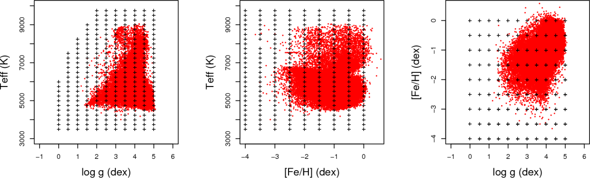
Figure 2: The grid of stellar atmospheric parameters $T_{\rm eff}$, $\log~{}g$, and ${\rm[Fe/H]}$. The synthetic parameters (plus symbols) are presented in comparison with previously estimated atmospheric parameters (dots) for 61 069 SDSS/SEGUE spectra.

In what follows, we focus on (normal) stars from the SDSS/SEGUE survey. From the observed stellar spectra, we derived models to estimate effective temperature, surface gravity, and metallicity via non linear regression models; these methods have been described in detail by [Re Fiorentin et al. (2007), Re Fiorentin et al. (2007)], to which the interested reader is referred for more details.

Basically, an ANN is used for parametrization by giving a functional mapping between PCA pre-processed stellar spectra as its inputs and the parameters at its outputs. Optimal mapping is achieved by training on a set of pre-classified observed data (e.g., [Lee et al. (2008), Lee et al. 2008]) and synthetic stellar templates derived from Kurucz’s model atmospheres; the grid of the available parameters is shown in Fig. 2.

From independent subsamples not involved in the training phase, the accuracies of our predictions (mean absolute errors) for each parameter are $T_{\rm eff}$ to $78$ K ($111$ K), $\log~{}g$ to $0.17$ dex ($0.31$ dex), and ${\rm[Fe/H]}$ to $0.09$ dex ($0.24$ dex), respectively. The precisions achieved now are about $50\%$ better than those reported in [Re Fiorentin et al. (2007), Re Fiorentin et al. (2007)], and are the result of further development of the regression models, improved stellar models, and better data calibrations.

Stellar atmospheric parameters are then derived for 186 580 stellar spectra (from SDSS/SEGUE plates) with signal-to-noise ratio $SNR>10$. This sample having, along with the photometry and radial velocities, is suitable to carry out Galactic studies; the following application is based on such a dataset.

4 Application: Stellar Properties of Galactic Tracers/Populations from SDSS

Here we illustrate the capability of an efficient classification and parameter estimation effort in the context of constraining Galaxy formation scenarios. Therefore, aiming to investigate the presence of substructures, we focus on Blue Horizontal-Branch (BHB) stars and RR Lyrae stars, which are excellent tracers to study Galactic populations, as they are nearly standard candles, and sufficiently bright to be detected up to large distances.

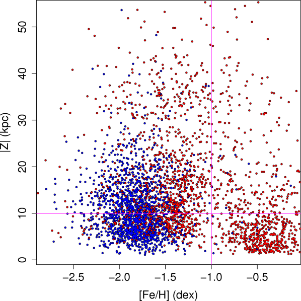
Figure 3: Metallicity distribution of the $4123$ stars selected as BHB (blue) or RR Lyrae (red), as a function of distance from the Galactic plane. Lines show constraints on the subsequent tracers selection.

Candidate selection and distance estimates

In order to obtain pure tracers samples with no (or little) contamination, we combine simple colour cuts with the spectroscopic or atmospheric parameter information.

Due to multiple observations of the same stars in different spectrographic plugplates, the spectro-photometric sample consists effectively of $168\,340$ unique objects for which the parameters assigned depend on the signal-to-noise level of the spectra.

The $2517$ BHB stars of our sample were identified employing a stringent approach which combines colour cuts previously established by [Yanny et al. (2000), Yanny et al. (2000)] with a set of Balmer-line profile selection criteria (see [Xue et al. (2008), Xue et al. 2008]; [Sirko et al. (2004), Sirko et al. 2004]). These tracers have the best constrained absolute magnitude ($M_{g}=0.7$) and thus allow the derivation of accurate photometric distances.

The $1606$ RR Lyrae stars of our sample were assembled from the colour selection method proposed by [ivezic, Ivezi$\rm{\acute{c}}$ et al. (2005)], adopting a completeness of $C=50\%$ and efficiency of $E=35\%$. This was then achieved by adopting the following cuts in parameter space: $6100$ K $<T_{\rm eff}<7400$ K and $3$ dex $<\log~{}g<4$ dex. The absolute magnitude of RR Lyrae stars correlate quite closely with metallicity ${\rm[Fe/H]}$; we adopt the empirical linear relation given by [Kinman et al. (2007), Kinman et al. (2007)] and estimate their distances.

Spatial and Metallicity Distribution

The observed magnitudes of our sample of $4123$ Galactic tracers have been used to infer their distances and, consequently, their Galactic distribution.

Figure 3 shows the metallicities and distances from the plane for BHB stars (blue) and RR Lyrae stars (red). Globally, we see a gradient of ${\rm[Fe/H]}$ with respect to $|Z|$. Inspection of this distribution shows the BHB and RR Lyrae stars as tracers having different intrinsic physical properties: while the former are essentially metal-poor halo stars that do not reach to the farthest distances, the latter include halo stars and old disk stars that extend deep into the outer halo. They represent the disk and halo populations which here appear remarkably well-defined and separated; the stellar properties obtained help describing such Galactic populations.

Furthermore, we can see possible clumps which suggest hints of substructures, the possible fossil signatures of past merging events. We are in the process of quantifying these via tests of clustering in spatial, metallicity, and radial velocity space.

5 Summary

We have implemented machine learning algorithms to classify observed objects and to determine their atmospheric parameters. Here, discrete source classifiers (from unsupervised and supervised analysis) are tested on RAVE spectra, and results for parameter estimation of single stars are given for SDSS/SEGUE spectra.

Based on the stellar atmospheric parameters which we have estimated from SDSS spectra we can better select target objects (such as BHB and RR Lyrae stars) for Galactic studies than by using photometry alone, and better explore the interface between the thick-disk and halo populations.

The models are in the process of development to improve their accuracy, and for the identification of peculiar/new types of objects, and their parameterization.

Looking further ahead, such strategies form the basis for future ground/space astrometric missions classifiers that are essential, in particular, for fully exploiting the astrometric part of the Gaia catalogue for stellar population studies.