Neutrino absorption by W production in the presence of a magnetic field

Abstract

In this work we calculate the decay rate of the electron type neutrinos into $W$ bosons and electrons in presence of an external uniform magnetic field. The decay rate is calculated from the imaginary part of the $W$ exchange neutrino self-energy diagram but in the weak field limit and compare our result with the existing one.

I Introduction

The topic of neutrino propagation in various non-trivial medium has been widely studied. Particularly the topic dealing with the passage of neutrinos through the cosmos or through some compact object containing a magnetic field is of particular interest. As magnetic fields are ubiquitous in our universe so when neutrinos travel from their point of creation to their destiny they may feel the effect of the magnetic fields. As the neutrinos we consider are standard model chiral neutrinos they do not posses any magnetic moment and the magnetic field affects them through virtual charged particles inside the loops of the neutrino self-energy diagrams Bhattacharya:2004nj ; Bhattacharya:2002aj ; D'Olivo:2002sp . It is known that in these circumstances the magnitude of the magnetic field which is required to affect the neutrino properties is relatively big, $O(10^{13}){\rm G}$. Such magnitude of magnetic fields are assumed to exist in neutron stars and magnetars. Consequently when neutrinos are produced in the neutron stars their properties can get modified because of the magnetic field. There has been many attempts to calculate the dispersion relation of neutrinos in presence of a magnetized medium, which employs the real part of the neutrino self-energy. But if we are trying to find out the absorption rate of the neutrinos then the imaginary part of the neutrino self-energy becomes important. There has been one attempt in the past Erdas:2002wk where the authors tried to calculate the absorption coefficient of the neutrinos in a magnetic field background. In their work, Erdas and Lissia Erdas:2002wk calculated the imaginary part of the self-energy of the neutrino, using the $W$ exchange diagram, and calculated the absorption coefficient of the neutrino when it decays into an electron $e^{-}$ and $W^{-}$ pair, in presence of a magnetic field. The present paper is aimed at calculating the damping rate of the neutrino due to its decay into $e^{-}$ and $W^{+}$ pair, in presence of a magnetic field. The quantities named absorption coefficient by Erdas and Lissia and damping rate by the present authors turn out to be the same, both related with the attenuation of a traveling neutrino in presence of a magnetic field. Our work estimates the damping rate of neutrinos when the neutrino propagation is damped due to its decay $\nu_{e}\to e^{-}+W^{+}$ in presence of a magnetic field. The threshold of the pair production process $\nu_{e}\to\nu_{e}+e^{-}+e^{+}$ in presence of a magnetic field has also been calculated Kuznetsov:1996vy ; Dicus:2007gb , and it is noted that the pair production threshold is smaller than the neutrino decay threshold. For higher energies of the neutrinos $O(10^{3-4}{\rm GeV)}$ and for magnetic field magnitude $O(10^{11-12}{\rm G})$ the neutrino decay rate becomes a prominent phenomena. The last reaction is kinematically forbidden in vacuum but can take place in presence of a magnetic field as in presence of a magnetic field the dispersion relation of the electron and positron changes. In their work Erdas and Lissia Erdas:2002wk calculated the imaginary part of the neutrino self-energy using the Feynman gauge for the $W$ boson propagator. In the present article we calculate the neutrino self-energy using the unitarity gauge. Our result is higher by 7% compared to the one by Erdas and Lissia.

The paper is organized as follows: In sec. 2, we have shown the relation between the damping rate and the imaginary part of the neutrino self-energy. In Sec. 3 we explain the terminology of the Schwinger proper time method and give the expression for the neutrino self energy due to W-exchange. The detail calculation of the imaginary part of the self-energy in the weak field limit and the damping rate are evaluated in Sec. 4. The threshold behavior as well as the asymptotic limit of the damping is also discussed in this section. A brief conclusion is given in Sec. 5. In appendix A we put some of the calculational details for the benefit of the reader.

II Damping rate of chiral fermions

In this section we briefly describe the main formula of the damping rate used in this paper. In general, the dispersion relation of a massless fermion with a momentum $k^{\mu}=(k^{0},\bf{k})$ is not given by $k^{0}=|\bf{k}|$ and in particular, $k^{0}$ is not zero at zero momentum. Writing

$$k^{0}=k_{r}^{0}-i\frac{\gamma}{2}\,,$$ (1)

where $k_{r}^{0}$ and $\gamma$ being real. The quantity $M=k_{r}^{0}(|\bf{k}|=0)$ is interpreted as an effective mass and $\gamma$ as the fermion damping rate. With the above convention the probability of the chiral fermion not to decay in a time period $t$ is $\sim e^{-\gamma t}$. The physically interesting regime is when $\gamma\ll k_{r}^{0}$, since otherwise the system would be over damped and the concept of a propagating mode is not meaningful. If we decompose the self-energy of the chiral fermion in real and imaginary parts as

$$\Sigma(k)={\rm Re}\Sigma(k)+i{\rm Im}\Sigma(k)\,,$$ (2)

the damping rate comes out to be D'Olivo:1993vm

$$\gamma=-\frac{1}{k^{0}}\bar{u}_{L}\,{\rm Im}\Sigma(k)\,u_{L}\,,$$ (3)

where the spinors $u_{L,R}$ satisfy the Dirac equation

$$({\hbox to0.0pt{k\hss}/}-{\rm Re}\Sigma(k))u_{L,R}=0\,.$$ (4)

Eqn. (3) can also be written as

$$\gamma=-\frac{1}{2k^{0}_{r}}{\rm Im}{\rm Tr}\,[{\hbox to0.0pt{k\hss}/}\Sigma(k)]\,,$$ (5)

where we treat the spinors as vacuum spinors and do neglect their corrections in the nontrivial media. In the present work we calculate the imaginary part of the self-energy of the standard model neutrino in presence of a strong magnetic field and using that result we find the damping rate of neutrino. To compare with earlier work we represent $\gamma$ in units of $m^{-1}$ and not in the traditional $s^{-1}$.

III The $W$ exchange diagram

Figure 1: The $W$ exchange diagram. The solid internal virtual lines represent modified propagator in presence of an external magnetic field.

If the weak SU(2) coupling constant is $g$ and the left-chiral projection operator is $L\equiv\frac{1}{2}(1-\gamma_{5})$ then the contribution to the neutrino self-energy from the $W$-boson exchange diagram is given by,

$$-i\Sigma_{W}(k)=\int\frac{d^{4}p}{(2\pi)^{4}}\left(-i\frac{g}{\sqrt{2}}\right)\gamma_{\mu}L\,iS_{e}(p)\left(-i\frac{g}{\sqrt{2}}\right)\gamma_{\nu}L\,\,iW^{\mu\nu}(q)+{\rm c.t.}$$ (6)

The c.t. is the counter term which has to be fed in the expression of the self-energy of the neutrino as the self-energy diagram contains ultraviolet divergence. The form of the c.t. is such that it cancels the divergence of the neutrino self-energy in the ${\mathcal{B}}\to 0$ limit. As the imaginary part of the self-energy in Eq. (6) is relevant for the calculation of $\nu_{e}\to W^{+}+e$ process so the c.t. will not affect our calculations as it does not contribute to the imaginary part of the self-energy. Consequently in this article we will not mention c.t. any further and write the self-energy of the neutrino in presence of a magnetic field as appearing in Eq. (6) without the counter term.

$S_{e}(p)$ is the electron propagator in presence of a magnetized medium and assuming the magnetic field to be along the $z$-axis of the coordinate system $S_{e}(p)$is given by:

$$iS_{e}(p)=\int^{\infty}_{0}ds_{1}\,\,e^{\phi(p,s_{1})}G(p,s_{1}).$$ (7)

The possible phase term in the electron propagator is not written as it will disappear in the one-loop calculation of the neutrino self-energy. In the above equation,

$$\phi(p,s_{1})=is_{1}(p_{0}^{2}-m^{2})-is_{1}(p_{3}^{2}+p_{\perp}^{2})\frac{\tan z_{1}}{z_{1}}-\epsilon|s_{1}|,$$ (8)

where $m$ is the mass of the electron and we have defined $z_{1}=|e|{\mathcal{B}}s_{1}$, $p_{\perp}^{2}=p_{1}^{2}+p_{2}^{2}$ and $\epsilon$ is an infinitesimal parameter introduced for the convergence of the integral in Eq. (7). Henceforth in this article we will not require the $\epsilon$ term explicitly and so it will not appear in further discussions. For the sake of writing the electron propagator in a covariant form two 4-vectors, $u^{\mu}$ and $b^{\mu}$, are used. As the magnetic field is a frame dependent quantity we assume in the rest frame of the observer $u^{\mu}$ is given by,

$$u^{\mu}=(1,{\bf 0})\,.$$ (9)

We have a uniform magnetic field along the $z$-axis. Likewise the effect of the magnetic field enters through the 4-vector $b^{\mu}$ which is defined in such a way that the frame in which $u^{\mu}=(1,{\bf 0})$ we have,

$$b^{\mu}=(0,\hat{\bf b})\,,$$ (10)

where we denote the magnetic field vector by ${\mathcal{B}}\hat{\bf b}$. With the help of these two 4-vectors the other term appearing in Eq. (7) can be written as,

$$G(p,s_{1})=\sec^{2}z_{1}\left[{\hbox to0.0pt{A\hss}/}+i{\hbox to0.0pt{B\hss}/}\gamma_{5}+m(\cos^{2}z-i\Sigma^{3}\sin z_{1}\cos z_{1})\right]\,,$$ (11)

where $A_{\mu}$ and $B_{\mu}$ stand for,

$$A_{\mu} = p_{\mu}-\sin^{2}z_{1}(p\cdot u\,\,u_{\mu}-p\cdot b\,\,b_{\mu})\,,$$ (12)

$$B_{\mu} = \sin z_{1}\cos z_{1}(p\cdot u\,\,b_{\mu}-p\cdot b\,\,u_{\mu})\,,$$ (13)

and

$$\Sigma^{3}=\gamma_{5}{\hbox to0.0pt{/\hss}b}{\hbox to0.0pt{/\hss}u}\,.$$ (14)

The momentum dependence of the propagator are shown in Fig. 1. The $W$ boson propagator in presence of a magnetic field is $W^{\mu\nu}(q)$ where $q=k-p$. In the weak-field limit i.e. $e{\mathcal{B}}\ll M_{W}^{2}$, the $W$-propagator is given by,

$$W_{\mu\nu}(q)=-\frac{1}{(q^{2}-M_{W}^{2})}\left[{\rm g}_{\mu\nu}-\frac{1}{M_{W}^{2}}(q_{\mu}q_{\nu}+\frac{ie}{2}F_{\mu\nu})\right]+\frac{2ieF_{\mu\nu}}{(q^{2}-M_{W}^{2})^{2}}\,.$$ (15)

The $q$ dependence of the terms in the denominator on the right hand side of the above equation can be expressed in integral form as

$$\frac{1}{(q^{2}-M_{W}^{2})} = -i\int_{0}^{\infty}ds_{2}\,\,e^{is_{2}(q^{2}-M_{W}^{2})}\,,$$ (16)

$$\frac{1}{(q^{2}-M_{W}^{2})^{2}} = -\int_{0}^{\infty}ds_{2}\,s_{2}\,\,e^{is_{2}(q^{2}-M_{W}^{2})}\,.$$ (17)

For convergence of the above integrals we require another term similar to the $\epsilon$ term in Eq. (7) which has not been explicitly written as it will never appear in further discussions. Using Schwinger’s proper time method the contribution to the neutrino self-energy coming from the $W$ exchange process can be expressed as,

$$\Sigma_{W}(k) = -\frac{ig^{2}}{2}\int\frac{d^{4}p}{(2\pi)^{4}}\,R\,\gamma_{\mu}S_{e}(p)\,\gamma_{\nu}\,L\,W^{\mu\nu}(q)$$ (18)

$$= -\frac{ig^{2}}{2}\int\frac{d^{4}p}{(2\pi)^{4}}\,R\,\gamma_{\mu}\int^{\infty}_{0}ds_{1}\int^{\infty}_{0}ds_{2}\,\,e^{\phi(p,s_{1})}\,G(p,s_{1})\,\gamma_{\nu}\,L\left[-{\rm g}^{\mu\nu}+\frac{1}{M_{W}^{2}}(q^{\mu}q^{\nu}+\frac{ie}{2}F^{\mu\nu})\right.$$

$$+ \left.2es_{2}F^{\mu\nu}\right]\,e^{is_{2}(q^{2}-M_{W}^{2})}\,.$$

As these integrals are lengthy and complicated to evaluate, we shall calculate them one by one.

IV $\Sigma_{W}(k)$ and the damping rate $\gamma$

In this section we will evaluate $\Sigma_{W}(k)$ given in Eq. (18). Before writing all the terms in $\Sigma_{W}(k)$ which will be evaluated separately at first we write down the phase appearing in the integrand on the right hand side of Eq. (18). Let us define,

$$\Delta = \phi(p,s_{1})+is_{2}(q^{2}-M_{W}^{2})$$ (19)

$$= -i(s_{1}m^{2}+s_{2}M_{W}^{2})+i(s_{1}+s_{2})(x_{0}^{2}-x_{3}^{2})-i\lambda(x_{1}^{2}+x_{2}^{2})-i\frac{z^{2}_{1}}{z_{1}+z_{2}}\frac{{k_{\parallel}}^{2}}{|e|B}+i\frac{z^{2}_{2}}{\lambda}\frac{{k_{\perp}}^{2}}{|e|B}\,,$$

where,

$$x_{0}=p_{0}-\frac{k_{0}s_{2}}{s_{1}+s_{2}},\, \,x_{3}=p_{3}-\frac{k_{3}s_{2}}{s_{1}+s_{2}},$$ (20)

$$x_{1}=p_{1}-\frac{k_{1}s_{2}}{\lambda},\,\,\,\,\,\,\,\, \,x_{2}=p_{2}-\frac{k_{2}s_{2}}{\lambda},$$ (21)

and

$$z_{i}=|e|{\mathcal{B}}s_{i}\,,\,\,\,\lambda=s_{1}\frac{\tan z_{1}}{z_{1}}+s_{2}.$$ (22)

Next the expression of $\Sigma_{W}(k)$ in Eq. (18) is decomposed into various parts which are evaluated separately. The decomposition of $\Sigma_{W}(k)$ is as follows:

$$\Sigma_{W}(k)=\Sigma^{(1)}_{W}(k)+\Sigma^{(2)}_{W}(k)+\Sigma^{(3)}_{W}(k)+\Sigma^{(4)}_{W}(k)\,,$$ (23)

where,

$$\Sigma^{(1)}_{W}(k) = \frac{ig^{2}}{2}\int\frac{d^{4}p}{(2\pi)^{4}}\,\int^{\infty}_{0}ds_{1}\int^{\infty}_{0}ds_{2}\,\,e^{\Delta}\,R\,\gamma_{\mu}\,G(p,s_{1})\,\gamma_{\nu}\,L\,{\rm g}^{\mu\nu}\,,$$ (24)

$$\Sigma^{(2)}_{W}(k) = -\frac{ig^{2}}{2M_{W}^{2}}\int\frac{d^{4}p}{(2\pi)^{4}}\,\int^{\infty}_{0}ds_{1}\int^{\infty}_{0}ds_{2}\,\,e^{\Delta}\,R\,\gamma_{\mu}\,G(p,s_{1})\,\gamma_{\nu}\,L\,q^{\mu}q^{\nu}\,,$$ (25)

$$\Sigma^{(3)}_{W}(k) = \frac{eg^{2}}{4M_{W}^{2}}\int\frac{d^{4}p}{(2\pi)^{4}}\,\int^{\infty}_{0}ds_{1}\int^{\infty}_{0}ds_{2}\,\,e^{\Delta}\,R\,\gamma_{\mu}\,G(p,s_{1})\,\gamma_{\nu}\,L\,F^{\mu\nu}\,,$$ (26)

$$\Sigma^{(4)}_{W}(k) = -ieg^{2}\int\frac{d^{4}p}{(2\pi)^{4}}\,\int^{\infty}_{0}ds_{1}\int^{\infty}_{0}ds_{2}\,s_{2}\,\,e^{\Delta}\,R\,\gamma_{\mu}\,G(p,s_{1})\,\gamma_{\nu}\,L\,F^{\mu\nu}\,.$$ (27)

Doing the Gaussian integrals in the momenta we can write Eq. (24) as,

$$\Sigma^{(1)}_{W}(k) = -\frac{g^{2}}{(4\pi)^{2}}\int^{\infty}_{0}ds_{1}\int^{\infty}_{0}ds_{2}\,e^{\Delta_{0}}\frac{1}{(s_{1}+s_{2})\lambda}R\left[\frac{s_{2}}{(s_{1}+s_{2})}{\not k}_{\parallel}+i\frac{s_{2}}{(s_{1}+s_{2})}(k_{0}{\hbox to0.0pt{b\hss}/}-k_{3}{\hbox to0.0pt{u\hss}/})\tan z_{1}\right.$$ (28)

$$- \left.\frac{s_{2}}{\lambda}{\not k}_{\perp}\sec^{2}z_{1}\right]L\,,$$

where,

$$\Delta_{0}=-i\frac{z^{2}_{2}}{(z_{1}+z_{2})}\frac{k^{2}_{\parallel}}{|e|B}+i\frac{z^{2}_{2}}{\lambda}\frac{k^{2}_{\perp}}{|e|B}-\frac{i}{|e|B}(z_{1}m^{2}+z_{2}M^{2})\,.$$ (29)

The expression in Eq. (25) can also be written as:

$$\Sigma^{(2)}_{W}(k) = -\frac{ig^{2}}{2M_{W}^{2}}\int\frac{d^{4}p}{(2\pi)^{4}}\,\int^{\infty}_{0}ds_{1}\int^{\infty}_{0}ds_{2}\,\,e^{\Delta}\,\sec^{2}z_{1}R\left[2q.(A+iB){\not q}-q^{2}({\hbox to0.0pt{A\hss}/}+i{\hbox to0.0pt{B\hss}/})\right]L\,,$$ (30)

$$= \Sigma^{(2a)}_{W}(k)+\Sigma^{(2b)}_{W}(k)\,,$$

where,

$$\Sigma^{(2a)}_{W}(k) = -\frac{ig^{2}}{2M_{W}^{2}}\int\frac{d^{4}p}{(2\pi)^{4}}\int^{\infty}_{0}ds_{1}\int^{\infty}_{0}ds_{2}\,\,e^{\Delta}\sec^{2}z_{1}R\left[2q.(A+iB){\hbox to0.0pt{q\hss}/}\right]L\,,$$ (31)

$$\Sigma^{(2b)}_{W}(k) = \frac{ig^{2}}{2M_{W}^{2}}\int\frac{d^{4}p}{(2\pi)^{4}}\int^{\infty}_{0}ds_{1}\int^{\infty}_{0}ds_{2}\,\,e^{\Delta}\sec^{2}z_{1}R\left[q^{2}({\hbox to0.0pt{A\hss}/}+i{\hbox to0.0pt{B\hss}/})\right]L\,.$$ (32)

The elaborate expressions of the above integrals are given in Appendix A. The evaluation of $\Sigma^{(3)}_{W}(k)$ and $\Sigma^{(4)}_{W}(k)$ are straight forward and completing the Gaussian integrals over the loop momenta we obtain:

$$\Sigma^{(3)}_{W}(k)=\frac{g^{2}}{2M^{2}}\frac{1}{(4\pi)^{2}}\int^{\infty}_{0}ds_{1}\int^{\infty}_{0}ds_{2}e^{\Delta_{0}}\frac{s_{2}}{(s_{1}+s_{2})^{2}\lambda}R\left[i(k_{0}{\not b}-k_{3}{\not u})-\tan z_{1}~{}{\not k}_{\parallel}\right]L\,,$$ (33)

and

$$\Sigma^{(4)}_{W}(k)=\frac{2eBg^{2}}{(4\pi)^{2}}\int^{\infty}_{0}ds_{1}\int^{\infty}_{0}ds_{2}e^{\Delta_{0}}\frac{s_{2}}{(s_{1}+s_{2})^{2}\lambda}R\left[i(k_{0}{\not b}-k_{3}{\not u})-\tan z_{1}~{}{\not k}_{\parallel}\right]L\,.$$ (34)

The damping rate of the neutrino is given by,

$$\gamma=-\frac{1}{2k_{0}}{\rm Im}~{}{\cal S}(k)\,,$$ (35)

where

$${\cal S}(k)={\rm Tr}[{\hbox to0.0pt{k\hss}/}\Sigma_{W}(k)]\,.$$ (36)

In Eq. (35) we have used the free dispersion relation of the neutrinos to write the neutrino energy in the denominator and consequently here we have $k_{r}^{0}\sim k^{0}$. The one-loop real part of the energy will differ from $k_{0}$ by factors proportional to the Fermi coupling $G_{F}$. For simplicity, we can change the integration variables from $(s_{1},s_{2})$ to $(z,u)$ where,

$$z=\frac{m^{2}}{eB}(z_{1}+z_{2})=\frac{1}{\beta}(z_{1}+z_{2})\,,$$ (37)

and

$$u=\frac{M_{W}^{2}}{m^{2}}\frac{z_{2}}{z_{1}+z_{2}}=\frac{1}{\eta}\frac{z_{2}}{z_{1}+z_{2}}\,.$$ (38)

With these new variables Eq. (29) can be written as:

$$\Delta_{0}=-iz\left[1-u\eta+u+u^{2}\eta\frac{k^{2}_{\perp}}{M_{W}^{2}}\left(1-\frac{\beta z}{\Omega}\right)\right]\,,$$ (39)

where we have defined:

$$\Omega=\tan~{}\beta z(1-u)+\beta zu\eta\,.$$ (40)

The phase $\exp(-iz)$ in $\exp(\Delta_{0})$ is oscillating and its main contribution to the $z$ integral will come from $z\leq 1$. Also for weak-field limit the condition is $eB\ll m^{2}$. So in the weak field limit the product $\beta z\ll~{}1$ and we can expand the terms in $\Sigma_{W}(k)$ up to second order in $\beta z$ (Appendix A contains the expression of $\Sigma^{(2)}_{W}(k)$). This gives:

$$\Delta_{0}\simeq-iz\left[1-u\eta+u+\frac{1}{3}\frac{k^{2}_{\perp}}{m^{2}}\left(\frac{eB}{M_{W}^{2}}\right)^{2}u^{2}z^{2}(1-u\eta)^{3}\right]\,.$$ (41)

As the $\Sigma^{i}$, for $i=1,2,3$ and $4$ are in the form:

$$\Sigma^{(i)}(k)=f_{1}{\hbox to0.0pt{k\hss}/}_{\parallel(\perp)}+f_{2}(k_{0}{\hbox to0.0pt{b\hss}/}-k_{3}{\hbox to0.0pt{u\hss}/})\,,$$ (42)

then from Eq. (36) we see that the trace

$${\rm Tr}[{\hbox to0.0pt{k\hss}/}(k_{0}{\hbox to0.0pt{b\hss}/}-k_{3}{\hbox to0.0pt{u\hss}/})]=0\,.$$ (43)

Consequently the terms which are proportional to ${\hbox to0.0pt{k\hss}/}_{\parallel(\perp)}$ will only contribute to the damping of the fermion. Also noting that for a massless neutrino ${\not k}=0$ and $k^{2}_{\parallel}=k^{2}_{\perp}$ we can write ${\cal S}$ in the weak field limit, where $\beta z\ll~{}1$, as:

$${\cal S}(k) \simeq -\frac{g^{2}k^{2}_{\perp}}{4\pi^{2}}\int^{\infty}_{0}dz\int^{1/\eta}_{0}du\,\,e^{\Delta_{0}}$$ (44)

$$\times \left[\frac{\beta^{2}\eta^{2}uz(u\eta-1)}{3}\left\{2u^{4}z^{2}\beta^{2}\eta^{4}-4u^{3}z^{2}\beta^{2}\eta^{3}+u^{2}(2z^{2}\beta^{2}-1)\eta^{2}+5u\eta+2\right\}\right.$$

$$- \left.\frac{i\beta^{2}\eta^{3}u(u\eta-1)}{90}\left\{z^{2}\beta^{2}(u\eta-1)^{2}~{}(100u^{3}\eta^{3}-252u^{2}\eta^{2}+129u\eta+8)+15(8u^{2}\eta^{2}-22u\eta+11)\right\}\right]\,.$$

¿From the above equation we can write,

$${\rm Im}{\cal S}(k)=\frac{(g\beta\eta)^{2}k^{2}_{\perp}}{12\pi^{2}}\int^{\infty}_{0}dz\int^{1/\eta}_{0}du\,u\,(u\eta-1)\left({\cal F}_{2}\cos D+{\cal F}_{1}\sin D\right)\,.$$ (45)

Here

$${\cal F}_{1}=z(2+5~{}u\eta-u^{2}\eta^{2})+2u^{2}\eta^{2}\beta^{2}z^{3}(1-2~{}u\eta+u^{2}\eta^{2})\,,$$

$${\cal F}_{2}=\frac{1}{2}\eta(11-22~{}u\eta+8u^{2}\eta^{2})+\frac{1}{30}\eta(u\eta-1)^{2}\beta^{2}z^{2}(8+129u\eta-252u^{2}\eta^{2}+100u^{3}\eta^{3})\,,$$ (46)

and

$$D=(1+u-u\eta)z+\frac{1}{3}\xi^{2}u^{2}(1-u\eta)^{3}z^{3}\,,$$ (47)

where we have defined

$$\xi=\frac{k_{\perp}}{m}\left(\frac{e{\cal B}}{M_{W}^{2}}\right).$$ (48)

By making the substitution

$$z=\frac{y}{(\xi u)^{2/3}(1-u\eta)}$$ (49)

we have

$$D=xy+\frac{1}{3}y^{3}\,,\,\,\,{\rm where}\,\,\,\,x=\frac{(1+u-u\eta)}{\xi^{2/3}u^{2/3}(1-u\eta)}\,.$$ (50)

In the new variable, ${\rm Im}{\cal S}(k)$ can be written as:

$${\rm Im}{\cal S}=-\frac{(g\beta\eta)^{2}k^{2}_{\perp}}{12\pi^{2}\xi^{\frac{2}{3}}}\int^{\infty}_{0}dy\int^{1/\eta}_{0}du\,u^{\frac{1}{3}}\left[{\cal F}_{2}\cos\left(xy+\frac{1}{3}y^{3}\right)+{\cal F}_{1}\sin\left(xy+\frac{1}{3}y^{3}\right)\right]\,.$$ (51)

In terms of the Airy function:

$$Ai(x)=\frac{1}{\pi}\int^{\infty}_{0}dy\cos\left(xy+\frac{1}{3}y^{3}\right)\,,$$ (52)

we can write Eq. (51) as:

$${\rm Im}{\cal S}(k)=-\frac{(g\beta\eta)^{2}k^{2}_{\perp}}{12\pi\xi^{\frac{2}{3}}}\int^{1/\eta}_{0}du\,\,u^{\frac{1}{3}}\left[(W_{0}-W_{2}~{}x+W_{3})Ai(x)-(W_{1}-W_{3}~{}x)Ai^{\prime}(x)\right]\,,$$ (53)

where

$$W_{0} = \frac{1}{2}\eta(11-22~{}u\eta+8u^{2}\eta^{2})\,,$$ (54)

$$W_{1} = \frac{(2+5~{}u\eta-u^{2}\eta^{2})}{1+u-u\eta}x\,,$$ (55)

$$W_{2} = \frac{\eta(u\eta-1)^{2}\beta^{2}(8+129u\eta-252u^{2}\eta^{2}+100u^{3}\eta^{3})}{30(1+u-u\eta)^{2}}x^{2}\,,$$ (56)

$$W_{3} = \frac{2u^{2}\eta^{2}\beta^{2}(1-2~{}u\eta+u^{2}\eta^{2})}{(1+u-u\eta)^{3}}x^{3}\,,$$ (57)

and $Ai^{\prime}(x)\equiv\frac{dAi(x)}{dx}$.

The numerical integration over $u$ shows that, it saturates much before reaching the value $1/\eta$, so here $u\eta\ll 1$ and we can neglect the terms with $u\eta$ or higher power of it in Eq. (53). So this gives

$${\rm Im}{\cal S}(k)\simeq-\frac{(g\beta\eta)^{2}k^{2}_{\perp}}{12\pi\xi^{\frac{2}{3}}}\int^{1/\eta}_{0}du\,\,u^{\frac{1}{3}}\left[\left(\frac{11\eta}{2}-\frac{4}{15}\frac{\eta\beta^{2}}{(1+u)^{2}}x^{3}\right)Ai(x)-\frac{2}{1+u}Ai^{\prime}(x)\right]\,,$$ (58)

with

$$x\simeq\frac{(1+u)}{(\xi u)^{2/3}}.$$ (59)

With these the damping rate of the neutrino is given as

$$\gamma=\frac{\sqrt{2}G_{F}k_{\perp}^{2}}{6\pi k_{0}\xi^{\frac{2}{3}}}\left(\frac{e{\cal B}}{M_{W}^{2}}\right)^{2}M_{W}^{2}\int_{0}^{1/\eta}du\,\,u^{\frac{1}{3}}\left[\eta\left(\frac{11}{2}-\frac{4}{15}\frac{\beta^{2}}{(1+u)^{2}}x^{3}\right)Ai(x)-\frac{2}{1+u}Ai^{\prime}(x)\right]\,.$$ (60)

As $\eta$ is much smaller than one we can henceforth neglect the part of the integrand proportional to $\eta$ and assume $1/\eta\sim\infty$. Also here we assume that $E_{\nu}=k_{0}\simeq k_{\perp}$ by taking $k_{3}$ to be very small and write the above equation as:

$$\gamma\sim-\frac{\sqrt{2}}{3\pi}G_{F}M^{2}_{W}E_{\nu}\left(\frac{{\cal B}}{{\cal B}_{c}}\right)^{2}\left(\frac{m}{M_{W}}\right)^{4}\xi^{-2/3}\int_{0}^{\infty}du\,\,\frac{u^{\frac{1}{3}}}{1+u}Ai^{\prime}(x)\,,$$ (61)

where ${\cal B}_{c}=m^{2}/e$ is the critical magnetic field. For the transverse neutrino energy $k_{\perp}$ above the threshold of $e$ and $W$ production, we have observed that the function

$$\xi^{-2/3}f(\xi)=-\xi^{-2/3}\int_{0}^{\infty}du\,\,\frac{u^{\frac{1}{3}}}{1+u}Ai^{\prime}(x) = \left(\frac{\xi^{-4/3}}{\sqrt{3}\pi}\right)\int^{\infty}_{0}\frac{du}{u^{1/3}}K_{2/3}\left(\frac{2}{3}\frac{(1+u)^{3/2}}{\xi u}\right),$$ (62)

$$\simeq 1.$$

In Eq. (62), we express the derivative of the Airy function in terms of modified Bessel function to compare the $u$ dependence of the integrand with Eq. (23) of ref.Erdas:2002wk , which has a different $u$ dependence and due to this our result differs from the result by Erdas et al., in the above reference. For neutrino energy much above the threshold, the damping rate behaves as

$$\gamma\simeq\frac{\sqrt{2}}{3\pi}G_{F}M^{2}_{W}E_{\nu}\left(\frac{{\cal B}}{{\cal B}_{c}}\right)^{2}\left(\frac{m}{M_{W}}\right)^{4},$$ (63)

which is same as the absorption coefficient calculated by Erdas et al, in ref.Erdas:2002wk .

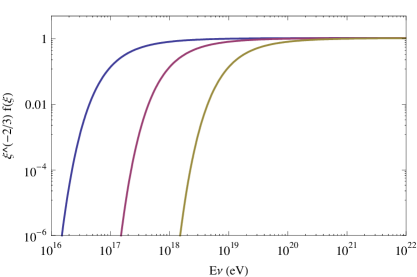
Figure 2: The Eq. (62) is plotted as a function of neutrino energy $E_{\nu}=k_{\perp}$ for different ${\cal B}$. From left to right, the curves are for ${\cal B}/{\cal B}_{c}$ =0.1, 0.01 and 0.001 respectively.

In Fig. 2, we have shown the behavior of Eq. (62) as a function of neutrino energy. For large $k_{\perp}$, it saturates at 1.065 and below the energy threshold below the function $\xi^{-2/3}f(\xi)$ increases very rapidly and saturates very fast. Because of this behavior the damping rate also increases very rapidly from very small value and after crossing the threshold the behavior becomes linear in neutrino energy. For small magnetic field, the saturation energy is larger than the one with larger magnetic field. As can be seen from the figure, for ${\cal B}/{\cal B}_{c}$ =0.1, the curve saturates around $k_{\perp}\simeq 10^{19}\,eV$, whereas for ${\cal B}/{\cal B}_{c}$ =0.001 the energy is about $10^{21}\,eV$. For the neutrino energy much above the threshold the asymptotic behavior is given in Eq. (63), where the damping rate is proportional to the neutrino energy and also it depends quadratically on the magnetic field as shown in the above equation. The behavior can be seen from Fig. 3, where we have plotted the damping rate as a function of energy for three different values (${\cal B}/{\cal B}_{c}=0.1,\,0.01$ and $0.001$) of the magnetic field. Again larger the magnetic field, larger is the damping rate and for neutrino energy smaller than the threshold one, the damping rate is suppressed but increases rapidly by increasing the energy.

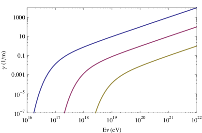
Figure 3: The damping rate is expressed in units of meter inverse is plotted against the transverse energy of the neutrino $E_{\nu}$. From the top to bottom are the curves for $B/B_{c}=0.1,\,0.01$ and $0.001$.

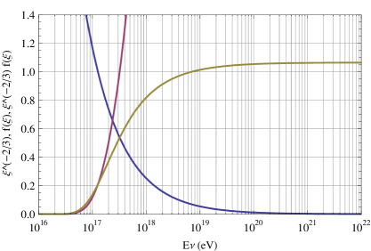
Figure 4: The functions $\xi^{-2/3}$, $f(\xi)$ and $\xi^{-2/3}f(\xi)$ are plotted as function of $E_{\nu}$ for ${\cal B}/{\cal B}_{c}=0.1$. The extreme left decreasing curve is the function $\xi^{-2/3}$, the second increasing curve is $f(\xi)$ and the third one which is saturated around 1 is the function $\xi^{-2/3}f(\xi)$.

The behavior of the process $\nu_{e}\rightarrow e^{-}+W^{+}$ solely depends on $\xi^{-2/3}f(\xi)$ and the threshold condition satisfies $\xi^{-2/3}f(\xi)<1$. We have analyzed the threshold behavior of the above process by taking into account the behavior of the functions $\xi^{-2/3}$, $f(\xi)$ and their product as function of neutrino energy, which are shown in Fig. 4 for ${\cal B}/{\cal B}_{c}=0.1$ and accurately find out the threshold energy. With increasing energy the function $\xi^{-2/3}$ decreases and $f(\xi)$ increases and both of them intersect at a point $\sim 0.66$ which lies before the saturation point of their product and this is the point of threshold. The estimated neutrino energy at this point is $E_{\nu}=2.37\times 10^{17}{\rm eV}$. We have observed that, for ${\cal B}/{\cal B}_{c}=0.01$ and $0.001$, the intersection point of the two functions as described above remains the same (0.66) but the neutrino energy shift towards higher values. For ${\cal B}/{\cal B}_{c}=0.01$, we obtain $E_{\nu}=2.37\times 10^{18}{\rm eV}$ and $2.37\times 10^{19}{\rm eV}$ respectively. For $\nu_{\mu}$ and $\nu_{\tau}$ decay calculations the electron mass has to be replaced by the corresponding lepton mass.

$$\xi=1.87\left(\frac{{\cal B}}{{\cal B}_{c}}\right),$$ (64)

or in terms of the above, we can write the threshold neutrino energy as

$$E^{th}_{\nu}=2.36\times 10^{16}\left(\frac{{\cal B}_{c}}{{\cal B}}\right)\,eV$$ (65)

which is about 7% higher than the one obtained by Erdas et. al.Erdas:2002wk .

V Conclusion

By using the Schwinger’s proper time electron propagator we calculate the imaginary part of the neutrino self energy in a constant magnetic field background. In this calculation we assume that the magnetic field to be weak $e{\cal B}\ll m^{2}$. From the imaginary part of the neutrino self energy we calculate the damping rate i.e. conversion of neutrino into electron and W-boson. We explicitly evaluated all the contributions in the weak field limit. We found that the behavior of the process $\nu_{e}\rightarrow e^{-}+W^{+}$ solely depends on the quantity $\xi^{-2/3}f(\xi)$. The threshold energy for this process can be accurately determined from the intersection of the functions $\xi^{-2/3}$ and $f(\xi)$ as functions of energy. Also for the neutrino energy much above the threshold we found that the damping rate is proportional to the neutrino energy and also it depends quadratically on the strength of the magnetic field. Our calculation gives an alternative way to arrive at the absorption cross-section calculated previously in Erdas:2002wk . The damping rate expressed in dimensions of inverse length matches to a reasonable degree with the old result although the gauge to fix the weak boson propagator is different in our case. This shows the gauge invariance of the calculations also.

Appendix

Appendix A The integral representation of the $W$ exchange diagram

The expression in Eq. (25) can also be written as:

$$\Sigma^{(2)}_{W}(k) = -\frac{ig^{2}}{2M_{W}^{2}}\int\frac{d^{4}p}{(2\pi)^{4}}\,\int^{\infty}_{0}ds_{1}\int^{\infty}_{0}ds_{2}\,\,e^{\Delta}\,\sec^{2}z_{1}R\left[2q.(A+iB){\not q}-q^{2}({\hbox to0.0pt{A\hss}/}+i{\hbox to0.0pt{B\hss}/})\right]L\,,$$ (66)

$$= \Sigma^{(2a)}_{W}(k)+\Sigma^{(2b)}_{W}(k)\,,$$

where,

$$\Sigma^{(2a)}_{W}(k) = -\frac{ig^{2}}{2M_{W}^{2}}\int\frac{d^{4}p}{(2\pi)^{4}}\int^{\infty}_{0}ds_{1}\int^{\infty}_{0}ds_{2}\,\,e^{\Delta}\sec^{2}z_{1}R\left[2q.(A+iB){\hbox to0.0pt{q\hss}/}\right]L\,,$$ (67)

$$\Sigma^{(2b)}_{W}(k) = \frac{ig^{2}}{2M_{W}^{2}}\int\frac{d^{4}p}{(2\pi)^{4}}\int^{\infty}_{0}ds_{1}\int^{\infty}_{0}ds_{2}\,\,e^{\Delta}\sec^{2}z_{1}R\left[q^{2}({\hbox to0.0pt{A\hss}/}+i{\hbox to0.0pt{B\hss}/})\right]L\,.$$ (68)

The term $q.(A+iB){\hbox to0.0pt{q\hss}/}$ in the integrand on the right hand side of Eq. (67) can be written in terms of $x_{0},\,x_{1},\,x_{2},\,x_{3}$ as,

$$q.(A+iB){\hbox to0.0pt{q\hss}/} = \left[d_{0}-x^{2}_{0}cos^{2}z_{1}+\lambda_{0}x_{0}+x^{2}_{1}+x^{2}_{2}+x^{2}_{3}\cos^{2}z_{1}+\frac{(x_{1}k_{1}+x_{2}k_{2})}{\lambda}\left(s_{2}-s_{1}\frac{\tan z_{1}}{z_{1}}\right)-\lambda_{3}x_{3}\right]$$ (69)

$$\times (a_{0}-\gamma_{0}x_{0}+\gamma_{1}x_{1}+\gamma_{2}x_{2}+\gamma_{3}x_{3})\,,$$

where,

$$a_{0}=\frac{s_{1}}{s_{1}+s_{2}}{k_{\parallel}}-\frac{s_{1}}{\lambda}\frac{\tan z_{1}}{z_{1}}k_{\perp}\,,\,\,\,d_{0}=\frac{s_{1}s_{2}}{(s_{1}+s_{2})^{2}}{k_{\parallel}}^{2}\cos^{2}z_{1}-\frac{s_{1}s_{2}}{\lambda^{2}}\frac{\tan z_{1}}{z_{1}}{k_{\perp}}^{2}\,,$$ (70)

and,

$$\lambda_{0}=\frac{(s_{1}-s_{2})}{(s_{1}+s_{2})}k_{0}\cos^{2}z_{1}+i\sin z_{1}~{}\cos z_{1}k_{3}\,,\,\,\,\lambda_{3}=\frac{(s_{1}-s_{2})}{(s_{1}+s_{2})}k_{3}\cos^{2}z_{1}+i\sin z_{1}~{}\cos z_{1}k_{0}\,.$$ (71)

where we have assumed that $k_{0}\simeq k_{\perp}$ by taking $k_{3}$ to be very small. Expressing the derivative of the Airy function in terms of Bessel function as

$$Ai^{\prime}(x)=-\frac{1}{\pi}\frac{x}{\sqrt{3}}K_{2/3}\left(\frac{2}{3}x^{3/2}\right),$$ (72)

we can express the damping rate as

$$\gamma = \frac{\sqrt{2}}{3\sqrt{3}}\frac{1}{\pi^{2}}G_{F}\frac{k^{2/3}_{\perp}}{k_{0}}(|e|{\cal B})^{2/3}(m^{2}M_{W})^{2/3}\int^{\infty}_{0}\frac{du}{u^{1/3}}K_{2/3}\left(\frac{2}{3}\frac{(1+u)^{3/2}}{\xi u}\right)$$ (73)

$$= \frac{\sqrt{2}}{3\pi}G_{F}M^{2}_{W}k_{\perp}\left(\frac{B}{B_{c}}\right)^{2}\left(\frac{m}{M_{W}}\right)^{4}\left(\frac{1}{\sqrt{3}\pi\xi^{4/3}}\right)\int^{\infty}_{0}\frac{du}{u^{1/3}}K_{2/3}\left(\frac{2}{3}\frac{(1+u)^{3/2}}{\xi u}\right),$$

In a similar fashion the term $q^{2}({\hbox to0.0pt{A\hss}/}+i{\hbox to0.0pt{B\hss}/})$ in Eq. (68) can be written as,

$$q^{2}({\hbox to0.0pt{A\hss}/}+i{\hbox to0.0pt{B\hss}/}) = \left[g_{0}+x^{2}_{0}-x^{2}_{1}-x^{2}_{2}-x^{2}_{3}-\frac{2s_{1}}{(s_{1}+s_{2})}x_{0}k_{0}+\frac{2s_{1}}{\lambda}\frac{tanz_{1}}{z_{1}}(x_{1}k_{1}+x_{2}k_{2})+\frac{2s_{1}}{s_{1}+s_{2}}x_{3}k_{3}\right]$$ (74)

$$\times (h+h_{0}x_{0}-\gamma_{1}x_{1}-\gamma_{2}x_{2}-h_{3}x_{3})\,,$$

where,

$$g_{0} = \left(\frac{s_{2}^{2}}{(s_{1}+s_{2})^{2}}-\frac{2s_{2}}{(s_{1}+s_{2})}\right){k_{\parallel}}^{2}-\left(\frac{s^{2}_{2}}{\lambda^{2}}-\frac{2s_{2}}{\lambda}\right){k_{\perp}}^{2}\,,$$ (75)

$$h = \frac{s_{2}}{s_{1}+s_{2}}{{\not k}_{\parallel}}\cos^{2}z_{1}-\frac{s_{2}}{\lambda}{{\not k}_{\perp}}+i\frac{s_{2}}{s_{1}+s_{2}}\sin z_{1}~{}\cos z_{1}(k_{0}{\hbox to0.0pt{b\hss}/}-k_{3}{\hbox to0.0pt{u\hss}/})\,,$$ (76)

and

$$h_{0}=\cos^{2}z_{1}{\hbox to0.0pt{u\hss}/}+i{\hbox to0.0pt{b\hss}/}\sin z_{1}~{}\cos z_{1}\,,\,\,\,h_{3}=\cos^{2}z_{1}{\hbox to0.0pt{b\hss}/}+i{\hbox to0.0pt{u\hss}/}\sin z_{1}~{}\cos z_{1}\,.$$ (77)

Using the expressions of $q.(A+iB){\hbox to0.0pt{q\hss}/}$ and $q^{2}({\hbox to0.0pt{A\hss}/}+i{\hbox to0.0pt{B\hss}/}\,)$ in Eqns. (67) and (68) and doing the $x_{i}$ integrals we obtain:

$$\Sigma^{(2a)}_{W}(k) = -\frac{g^{2}}{M_{W}^{2}}\frac{1}{(4\pi)^{2}}\int^{\infty}_{0}ds_{1}\int^{\infty}_{0}ds_{2}\,\,e^{\Delta_{0}}\frac{\sec^{2}z_{1}}{(s_{1}+s_{2})\lambda}$$ (78)

$$\times R\left[{\hbox to0.0pt{k\hss}/}_{\parallel}\left\{\left(\frac{s^{2}_{1}s_{2}}{(s_{1}+s_{2})^{3}}k^{2}_{\parallel}\cos^{2}z_{1}-\frac{s^{2}_{1}s_{2}}{(s_{1}+s_{2})\lambda^{2}}k^{2}_{\perp}\frac{\tan z_{1}}{z_{1}}\right)-i\left(\frac{2s_{1}}{(s_{1}+s_{2})\lambda}+\frac{(3s_{1}-s_{2})}{(s_{1}+s_{2})^{2}}\cos^{2}z_{1}\right)\right\}\right.$$

$$\left.+{\hbox to0.0pt{k\hss}/}_{\perp}\left\{\left(\frac{s^{2}_{1}s_{2}}{\lambda^{3}}\frac{\tan^{2}z_{1}}{z^{2}_{1}}{k_{\perp}}^{2}-\frac{s^{2}_{1}s_{2}}{(s_{1}+s_{2})^{2}\lambda}\frac{\sin z_{1}~{}\cos z_{1}}{z_{1}}\right)\right.\right.$$

$$\left.\left.+i\left(\frac{2s_{1}}{(s_{1}+s_{2})\lambda}\frac{\sin z_{1}~{}\cos z_{1}}{z_{1}}+\frac{1}{\lambda^{2}}(3s_{1}\frac{\tan z_{1}}{z_{1}}-s_{2})\right)\right\}+(k_{3}{\hbox to0.0pt{u\hss}/}-k_{0}{\hbox to0.0pt{b\hss}/})\frac{\sin z_{1}~{}\cos z_{1}}{s_{1}+s_{2}}\right]L\,,$$

$$\Sigma^{(2b)}_{W}(k) = \frac{g^{2}}{2M_{W}^{2}}\frac{1}{(4\pi)^{2}}\int^{\infty}_{0}ds_{1}\int^{\infty}_{0}ds_{2}\,\,e^{\Delta_{0}}\frac{sec^{2}z_{1}}{(s_{1}+s_{2})\lambda}$$ (79)

$$\times R\left[{\hbox to0.0pt{k\hss}/}_{\parallel}\left\{\left(-\frac{(2s_{1}+s_{2})}{(s_{1}+s_{2})^{3}}k^{2}_{\parallel}+\frac{s^{2}_{2}}{(s_{1}+s_{2})\lambda^{2}}\left(2s_{1}\frac{\tan z_{1}}{z_{1}}k^{2}_{\perp}\right)\right)\cos^{2}z_{1}-2i\cos^{2}z_{1}\left(\frac{s_{1}-s_{2}}{(s_{1}+s_{2})^{2}}-\frac{s_{2}}{(s_{1}+s_{2})\lambda}\right)\right\}\right.$$

$$\left.+{\hbox to0.0pt{k\hss}/}_{\perp}\left\{\left(-\frac{s^{2}_{2}}{\lambda^{3}}\left(2s_{1}\frac{\tan z_{1}}{z_{1}}k^{2}_{\perp}\right)k^{2}_{\parallel}+\frac{s^{2}_{2}}{\lambda}\frac{(2s_{1}+s_{2})}{(s_{1}+s_{2})^{2}}\right)-i\left(\frac{2s_{2}}{(s_{1}+s_{2})\lambda}+\frac{2s_{2}}{\lambda^{2}}-\frac{2s_{1}}{\lambda}\frac{\tan z_{1}}{z_{1}}\right)\right\}\right.$$

$$\left.+(k_{0}{\hbox to0.0pt{b\hss}/}-k_{3}{\hbox to0.0pt{u\hss}/})\frac{s_{2}}{s_{1}+s_{2}}\sin z_{1}~{}\cos z_{1}\left\{\left(\frac{2s_{1}}{s_{2}(s_{1}+s_{2})}-\frac{2}{(s_{1}+s_{2})}-\frac{2}{\lambda}\right)\right.\right.$$

$$\left.\left.-i\left(\frac{s_{2}(2s_{1}+s_{2})}{(s_{1}+s_{2})^{2}}k^{2}_{\parallel}-\frac{2s_{1}s_{2}}{\lambda^{2}}\frac{\tan z_{1}}{z_{1}}k^{2}_{\perp}\right)\right\}\right]L\,.$$

This results are used to evaluate $\Sigma^{(2)}_{W}(k)$.

References

• (1) K. Bhattacharya, Ph. D. Thesis, arXiv:hep-ph/0407099.
• (2) K. Bhattacharya and P. B. Pal, Proc. Indian Natl. Sci. Acad.  70, 145 (2004) [arXiv:hep-ph/0212118].
• (3) J. C. D’Olivo, J. F. Nieves and S. Sahu, Phys. Rev.  D 67, 025018 (2003) [arXiv:hep-ph/0208146].
• (4) A. Erdas and M. Lissia, Phys. Rev.  D 67, 033001 (2003) [arXiv:hep-ph/0208111].
• (5) A. V. Kuznetsov and N. V. Mikheev, Phys. Lett.  B 394, 123 (1997) [arXiv:hep-ph/9612312].
• (6) D. A. Dicus, W. W. Repko and T. M. Tinsley, Phys. Rev.  D 76, 025005 (2007) [Erratum-ibid.  D 76, 089903 (2007)] [arXiv:0704.1695 [hep-ph]].
• (7) A. Bravo Garcia, K. Bhattacharya and S. Sahu, arXiv:0706.3921 [hep-ph].
• (8) A. Erdas and G. Feldman, Nucl. Phys.  B 343, 597 (1990).
• (9) J. C. D’Olivo and J. F. Nieves, Phys. Rev.  D 52, 2987 (1995) [arXiv:hep-ph/9309225].