Even-odd effects in finite Heisenberg spin chains

Abstract

Magnetic superlattices and nanowires may be described as Heisenberg spin chains of finite length $N$, where $N$ is the number of magnetic units (films or atoms, respectively). We study antiferromagnetically coupled spins which are also coupled to an external field $H$ (superlattices) or to a ferromagnetic substrate (nanowires). The model is analyzed through a two-dimensional map which allows fast and reliable numerical calculations. Both open and closed chains have different properties for even and odd $N$ (parity effect). Open chains with odd $N$ are known [S. Lounis et al., Phys. Rev. Lett. 101, 107204 (2008)] to have a ferrimagnetic state for small $N$ and a noncollinear state for large $N$. In the present paper, the transition length $N_{c}$ is found analytically. Finally, we show that closed chains arrange themselves in the uniform bulk spin-flop state for even $N$ and in nonuniform states for odd $N$.

Antiferromagnetic (AF) chains of Heisenberg spins, when subjected to an external magnetic field (and possibly to a uniaxial anisotropy), are known to arrange themselves in a spin-flop (SF) state where neighboring spins are almost antiparallel and orthogonal to the field Neel . However, such a result is valid, strictly speaking, only in the thermodynamic limit. For a finite chain, boundary conditions and finite size effects are expected to induce modifications on the bulk spin-flop configuration, determining a non uniform canting along the chain.

A one-dimensional (1D) classical planar model of a Heisenberg uniaxial antiferromagnet,

$${\cal H}_{AF} = \sum_{i=1}^{N-1}H_{E}\cos(\theta_{i}-\theta_{i+1})$$ (1)

$$- \sum_{i=1}^{N}(H_{A}\cos^{2}\theta_{i}+2H\cos\theta_{i}),$$ (2)

was introduced forty years ago Mills to study a semi-infinite AF chain ($N\to\infty$). In Eq. (1), $H_{E}$ denotes the exchange field, $H_{A}$ the anisotropy field, and $\theta_{i}$ is the angle that the magnetization of the $i$-th ferromagnetic layer forms with the direction of the external field, $H$ (spins are assumed to be planar). The bulk SF phase appears for $H>\sqrt{2H_{E}H_{A}+H_{A}^{2}}$ ($H>0$ for zero anisotropy $H_{A}$).

At that time, the reference experimental systems were bulk systems like MnF₂ or MnO, with magnetic ions on special crystallographic planes interacting ferromagnetically (FM) and ions between planes interacting AF. With the spreading of epitaxially grown systems, the model was used a lot WangMillsPRL ; WangMillsPRB ; PRL ; JAP ; IJMPB ; Bogdanov to study superlattices made of $N$ ferromagnetic layers which are antiferromagnetically coupled. Some important theoretical results were found: (i) For semi-infinite systems, the surface SF state (a phase predicted to anticipate the bulk SF state when increasing the field) does not exist PRL ; (ii) For finite systems, there are important differences between structures with even and odd $N$ WangMillsPRL ; WangMillsPRB ; JAP ; IJMPB .

Recently, the model of a finite 1D quantum Heisenberg antiferromagnet

$${\cal H}_{q}=|J_{1}|\sum_{i=1}^{N-1}{\bf S}_{i}\cdot{\bf S}_{i+1}$$ (3)

has gained new interest since it has been used to describe an AF nanowire deposited on a thin insulating layer Science . Paradigmatic examples of such a system are linear chains of 1 to 10 Mn atoms epitaxied on a CuN substrate Science . From the analysis of spin excitations of coupled atomic spins in the dimer and in the trimer ($N=2,3$), the Mn-Mn exchange interaction was found Science to be antiferromagnetic ($|J_{1}|=6.2$ meV) and the spin value to be $S=5/2$, identical to the spin of a free Mn atom. Using these parameters in Eq. (3), the magnetic behavior of longer wires could successfully be fitted Science .

When such AF Mn nanowires are deposited on a ferromagnetic layer, like Ni(001), an interesting frustration phenomenon occurs, since the exchange coupling between an adsorbed Mn spin and the magnetic moment of an underlying Ni atom of the substrate is ferromagnetic LounisPRB ; LounisPRL , $J_{2}>0$, and thus competes notaLounis with the Mn-Mn antiferromagnetic exchange, $J_{1}<0$. Therefore, in a classical spin approximation, one is led to consider the model LounisPRL

$${\cal H}_{N}=|J_{1}|\sum_{i=1}^{N-1}\cos(\theta_{i}-\theta_{i+1})-J_{2}\sum_{i=1}^{N}\cos\theta_{i},$$ (4)

where $\theta_{i}$ denotes the angle that the $i$-th spin of the AF nanowire forms with respect to the magnetization of the ferromagnetic substrate. Since the coupling $J_{2}$ is localized on the $i$-th site, it is apparent that it plays the same role as the magnetic field $2H$ in Eq. (1), while $|J_{1}|$ has to be identified with $H_{E}$, and $H_{A}$ (the uniaxial anisotropy) is zero. Therefore, when $N$ is finite and open boundary conditions are assumed, the existence of different ground states for odd $versus$ even $N$ is a well-known result WangMillsPRL ; IJMPB . Different ground states also reflect on different behaviors for the spin wave excitations WangMillsPRB ; JAP .

In a recent Letter LounisPRL S. Lounis et al., using both ab initio results and solutions to the classical Heisenberg model (4), confirmed that the ground state of finite AF nanowires deposited on ferromagnets depends on the parity of the number $N$ of atoms. They also found that, while even chains always have a noncollinear (NC) ground state, for odd $N$ a transition from a collinear ferrimagnetic (FI) to a NC configuration occurs when the chain length $N$ exceeds a critical value $N_{c}$. For example, using an iterative numerical scheme in order to minimize Eq. (4), the transition length was estimated LounisPRL to be 9 atoms for Mn chains on Ni(001).

Here we show that the classical Heisenberg model (4) can be investigated with great numerical and analytical profit in terms of a two-dimensional (2D) map method PRL ; JAP ; IJMPB ; Aubry ; Bak ; Belorov ; Pandit . Such an approach allows a fast and exact determination of the ground state configuration of finite chains and to find an analytical expression for the transition length for odd open chains.

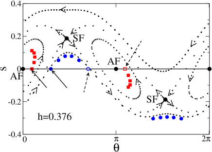
Figure 1: (color online) Phase portrait for mapping (5). Full red squares and blue circles correspond to equilibrium configurations for open chains with $N=9$ and $N=10$, respectively. Full arrows point to the values $\theta_{1}$ for the first atom of the chains. Dashed arrows point to the values $\theta_{N+1}$ (denoted by open symbols) for the fictitious $(N+1)$-th atom. Arrow tips allow one to follow the evolution of the map, whose hyperbolic and elliptic fixed points of order two, respectively denoted by SF and AF, correspond to uniform states.

By the map method, we also study model (4) in the case of periodic boundary conditions. For such “closed” chains, we find a new even-odd effect: even chains have spins arranged in the spin-flop state, like infinite chains, while odd chains arrange themselves in noncollinear states.

In order to find the equilibrium configurations of the classical Heisenberg model (4) by the 2D map method, we introduce Belorov the variable $s_{n}=\sin(\theta_{n}-\theta_{n-1})$. Denoting by $h=J_{2}/|J_{1}|$ the ratio between competing exchange interactions, minimization of (4) gives note_sin

$$s_{n+1}=s_{n}-h\sin\theta_{n},\hbox{~{}~{}~{}}\theta_{n+1}=\theta_{n}+\sin^{-1}(s_{n+1}).$$ (5)

These equations define an iterative 2D map Ott , i.e. point $(\theta,s)$ in the phase space is mapped to a point $(\theta^{\prime},s^{\prime})$. The fixed points of order two ($s_{n+2}=s_{n}$ and $\theta_{n+2}=\theta_{n}$) correspond to the collinear AF configuration ($(0,0)\leftrightarrow(\pi,0)$) and to the bulk SF state ($(\bar{\theta},\sin 2\bar{\theta})\leftrightarrow(-\bar{\theta},-\sin 2\bar{\theta})$, with $\cos\bar{\theta}=h/4$). In Fig. 1 we plot the fixed points and the evolution of the map for different initial conditions and $h=0.376$ (it is the special value considered in Ref. LounisPRL, as representative of AF Mn nanowires on Ni(001)).

Boundary conditions for open chains of $N$ atoms are taken into account PRL ; Pandit by introducing a fictitious $(N+1)$-th atom and imposing $s_{1}=0=s_{N+1}$. The determination of the ground state therefore corresponds to finding the value $\theta_{1}$ such that, iterating the map $N$ times from the point $P_{1}=(\theta_{1},0)$, we get a point $P_{N+1}=(\theta_{N+1},0)$, with both $P_{1}$ and $P_{N+1}$ located on the horizontal axis, $s=0$. The $N$ values $\theta_{1},\dots,\theta_{N}$ then give the sought-after equilibrium configuration. In Fig. 1 we also plot the first $N$ steps of the map evolution giving the ground states for $N=9$ (red solid squares) and $N=10$ (blue solid circles). Different behaviors for even and odd $N$ can be inferred from the different location of their trajectories in the phase portrait. The configurations are explicitly shown in Fig. 2.

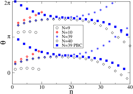
Figure 2: (color online) Equilibrium configurations $\theta_{1},\dots,\theta_{N}$ calculated by the 2D map method for open chains with $N=9,10,39,40$, and for a closed chain (PBC) with $N=39$.

Figure 3: (color online) We plot $s_{N+1}(\theta_{1})$, assuming $s_{1}=0$, for different, small values of $N$ (main figure) and for $N=39$ (inset). The arrows point to the equilibrium values $\theta_{1}$ for the first atom of the $N=9$ chain (red full line, full arrow) and of the $N=2$ chain (dashed line, dashed arrow).

The existence of a minimum length to get a noncollinear configuration for odd $N$ is clear from Fig. 3, where we plot $s_{N+1}$ as a function of $\theta_{1}$, assuming $s_{1}=0$. For odd $N<9$, the only zeros are the AF fixed points, corresponding to a collinear ferrimagnetic (FI) configuration, but for $N=9$, $ds_{N+1}/d\theta_{1}$ changes sign at $\theta_{1}=0$, and an additional solution appears: the noncollinear (NC) configuration. For even $N$, non trivial solutions exist already for $N=2$ (dashed line). The Inset of Fig. 3 shows that for large $N$ the function $s_{N+1}(\theta_{1})$ is strongly oscillating with several zeros $\theta_{1}^{(k)}$. In order to determine the ground state, the energies of all the NC configurations with $\theta_{1}=\theta_{1}^{(k)}$ must be compared.

We are now going to show that, by linearizing the map nearby the fixed points, it is indeed possible to determine the exact analytical condition for the rising of the NC state in the case of an open chain with odd $N$. If we start from a point $P_{1}=(s_{1},\theta_{1})$ close to the fixed point $(0,0)$, iterated points on the map are oscillating between the AF fixed points: more precisely, even $P_{2k}$ are close to $(\pi,0)$ and odd $P_{2k+1}$ are close to $(0,0)$. So, if we write

$$\theta_{2k} = \pi+\delta_{2k}$$ (6)

$$\theta_{2k+1} = \delta_{2k+1}$$ (7)

the quantities $\delta_{n}$ are small for any $n$, as $s_{n}$ are. Now, we can linearize the map in the two cases $P_{2k-1}\to P_{2k}$ and $P_{2k}\to P_{2k+1}$. If we write

$$\left(\begin{array}[]{c}\delta_{2k}\\ s_{2k}\end{array}\right)=A_{1}\left(\begin{array}[]{c}\delta_{2k-1}\\ s_{2k-1}\end{array}\right)\hbox{~{}~{}and~{}~{}}\left(\begin{array}[]{c}\delta_{2k+1}\\ s_{2k+1}\end{array}\right)=A_{2}\left(\begin{array}[]{c}\delta_{2k}\\ s_{2k}\end{array}\right)$$

we get the matrices

$$A_{1}=\left(\begin{array}[]{cc}1+h&-1\\ -h&1\end{array}\right)\hbox{~{}~{}and~{}~{}}A_{2}=\left(\begin{array}[]{cc}1-h&-1\\ h&1\end{array}\right).$$

So, if $N=2N_{0}+1$ is an odd integer, we have

$$\left(\begin{array}[]{c}\delta_{N+1}\\ s_{N+1}\end{array}\right)=A_{1}(A_{2}A_{1})^{N_{0}}\left(\begin{array}[]{c}\delta_{1}\\ s_{1}\end{array}\right)\equiv T\left(\begin{array}[]{c}\delta_{1}\\ s_{1}\end{array}\right).$$

Since $s_{N+1}=T_{21}\delta_{1}+T_{22}s_{1}$, if we start with $s_{1}=0$, the condition $ds_{N+1}/d\theta_{1}=ds_{N+1}/d\delta_{1}=0$ reads $T_{21}=0$. Let us now implement this condition, firstly determining eigenvalues $\lambda_{i}$ and eigenvectors $v_{i}$ of the matrix

$$A=A_{2}A_{1}=\left(\begin{array}[]{cc}1+h-h^{2}&h-2\\ h^{2}&1-h\end{array}\right).$$

It is easily found that

$$\lambda_{1,2} = \hbox{${1\over 2}$}(2-h^{2}\pm ih\sqrt{4-h^{2}})$$ (8)

$$v_{j} = \left(\begin{array}[]{c}{\lambda_{j}+h-1\over h^{2}}\\ 1\end{array}\right)\equiv\left(\begin{array}[]{c}v_{1j}\\ 1\end{array}\right)~{}~{}~{}j=1,2.$$ (13)

If $U$ is the $(2\times 2)$ matrix with $v_{1,2}$ as column vectors and $A_{D}$ is the diagonal matrix with elements $\lambda_{1,2}$, it is straightforward to write $T=A_{1}UA_{D}^{N_{0}}U^{-1}$. Finally, the condition $T_{21}=0$ gives

$$h(v_{11}\lambda_{1}^{N_{0}}-v_{12}\lambda_{2}^{N_{0}})=\lambda_{1}^{N_{0}}-\lambda_{2}^{N_{0}},$$ (14)

which simplifies to

$$\left({\lambda_{1}\over\lambda_{2}}\right)^{N_{0}}={\lambda_{2}-1\over\lambda_{1}-1}.$$ (15)

Therefore, the transition length is equal to $N_{c}=2N_{0}+1$ where $N_{0}$ is the solution of the above equation. We get

$$N_{c}={\pi\over\varphi},$$ (16)

with

$$\cos\varphi={2-h^{2}\over 2}~{}~{}~{}~{}~{}\sin\varphi={h\sqrt{4-h^{2}}\over 2}.$$ (17)

The curve is plotted as circles in Fig. 4 along with the asymptotic form $N_{c}=\pi/h$ (full line) which appears to be a very good approximation even for small $N$ (see the Inset).

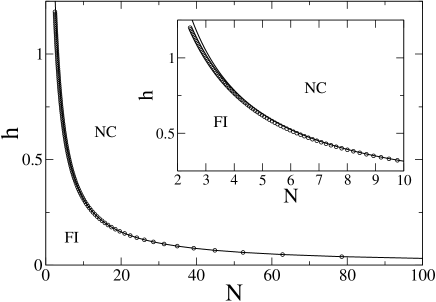
Figure 4: Main: analytical results of the phase diagram for odd-$N$ open chains, Eqs. (16-17). FI and NC denote FerrImagnetic and NonCollinear states. The full line is the curve $h_{c}=\pi/N$ which is a very good approximation, even for small $N$ (Inset).

We now turn to closed chains, which imply periodic boundary conditions (PBC). If spins represent magnetic layers, these boundary conditions are not physical, but for nanowires deposited on a substrate they are physical and correspond to nanorings. In terms of the 2D mapping, PBC imply $P_{N+1}\equiv P_{1}$, i.e. $\theta_{N+1}=\theta_{1}$ and $s_{N+1}=s_{1}$. Therefore, trajectories are fixed points of order $N$. It is easy to realize that the ground state for even $N$ is the bulk spin-flop state: $\theta_{2k}=\bar{\theta}$ and $\theta_{2k+1}=-\bar{\theta}$, with $\cos\bar{\theta}=h/4$. In fact, if $\theta_{1},\dots,\theta_{N}$ were a different configuration with a lower energy, we might replicate it indefinitely for an infinite chain and get a configuration with an energy lower than the bulk spin-flop phase (which is the ground state).

The above argument does not apply to odd $N$, because the SF phase, as well as the AF phase, which are fixed points of order two, do not satisfy PBC for odd $N$. In this case, we have a nonuniform state. In order to find it, we should look for the points $P$ that are iterated on themselves after $N$ applications of the map. It appears that the configuration is symmetric with respect to the field direction, i.e. for any spin with an angle $\theta^{*}$ there is a spin forming an angle $-\theta^{*}$, see Fig. 5 for $N=9$. Therefore, for odd $N$, there is one spin with $\theta=0$. PBC allow to label this spin as “number 1”, so that searching the solution is now as easy as for open chains: we apply the map $N$ times to points $(0,s_{1})$ and look for the values $s_{1}$ such that $\theta_{N+1}=0$ and $s_{N+1}=s_{1}$. Using this method, we have found the ground state for $N=39$ (Fig. 2, full squares) and for $N=9$ (Fig. 5).

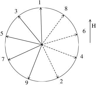
Figure 5: Graphical representation of the ground state for a closed chain with $N=9$. Full and dashed arrows represent spin orientations on odd and even sites, respectively. $\theta_{1}=0$ and for every angle $\theta_{2k}$ there is an angle $\theta_{2j+1}=-\theta_{2k}$.

In conclusion, we have studied model (4) which describes a chain of classical planar spins with nearest neighboring AF coupling and interacting with a (real or effective) external field $h$. Since the anisotropy is zero, the infinite system is in the bulk SF phase for any nonvanishing $h$. Extrema of the energy correspond to trajectories of the 2D mapping (5) with appropriate boundary conditions: $s_{1}=s_{N+1}=0$ for open chains and $\theta_{N+1}=\theta_{1},s_{N+1}=s_{1}$ for closed chains.

This method allows a fast and exact determination of the ground states for any $N$ (Fig. 2). It also allows to find analytically the transition length $N_{c}$ for open odd chains from the FI to the NC state (Fig. 4). This transition corresponds to a change in sign of the derivative $ds_{N+1}/d\theta_{1}$ at $\theta_{1}=0$ (Fig. 3). Parity effects are present for open and closed chains.

With increasing the field $h$, the 2D map starts developing a chaotic behavior Bogdanov ; chaos . Studying this regime with reference to nanowires would be an interesting subject for future work.

References

- (1) L. Néel, Ann. Phys. (Paris) 5, 232 (1936).
- (2) D. L. Mills, Phys. Rev. Lett. 20, 18 (1968).
- (3) R. W. Wang, D. L. Mills, E. E. Fullerton, J. E. Mattson, and S. D. Bader, Phys. Rev. Lett. 72, 920 (1994).
- (4) R. W. Wang and D. L. Mills, Phys. Rev. B 50, 3931 (1994).
- (5) L. Trallori, P. Politi, A. Rettori, M. G. Pini, and J. Villain, Phys. Rev. Lett. 72, 1925 (1994).
- (6) L. Trallori, P. Politi, A. Rettori, M. G. Pini, and J. Villain, J. Appl. Phys. 76, 6555 (1994).
- (7) L. Trallori, M. G. Pini, A. Rettori, M. Macciò, and P. Politi, Int. J. Mod. Phys. B 10, 1935 (1996).
- (8) U. K. Rössler and A. N. Bogdanov, Phys. Rev. B 69, 094405 (2004).
- (9) C. F. Hirjibehedin, C. P. Lutz, and A. J. Heinrich, Science 312, 1021 (2006).
- (10) S. Lounis, Ph. Mavropoulos, P. H. Dederichs, and S. Blügel, Phys. Rev. B 72, 224437 (2005).
- (11) S. Lounis, P. H. Dederichs, and S. Blügel, Phys. Rev. Lett. 101, 107204 (2008).
- (12) Notice that frustration occurs also in the case of antiferromagnetic exchange coupling between an atom of the AF wire and a magnetic moment of the ferromagnetic substrate, as is the case of AF Cr wires deposited on Ni(001) LounisPRB .
- (13) S. Aubry, in Solitons and Condensed Matter Physics, edited by A. R. Bishop and T. Schneider (Springer, 1979).
- (14) P. Bak, Phys. Rev. Lett. 46, 791 (1981).
- (15) P. I. Belorov et al., Zh. Eksp. Teor. Fiz. 87, 310 (1984) [Sov. Phys. JETP 60, 180 (1984)].
- (16) R. Pandit and M. Wortis, Phys. Rev. B 25, 3226 (1982).
- (17) The function is a two-values function. The correct value Belorov is within and .
- (18) E. Ott, Chaos in Dynamical Systems (Cambridge University Press, 2002).
- (19) L. Trallori, P. Politi, A. Rettori, M.G. Pini, and J. Villain, J. Phys.: Cond. Matt. 7, L451 (1995).