Electronic and transport properties of rectangular graphene macromolecules and zigzag carbon nanotubes of finite length

Abstract

We study one dimensional (1D) carbon ribbons with the armchair edges and the zigzag carbon nanotubes and their counterparts with finite length (0D) in the framework of the Hückel model. We prove that a 1D carbon ribbon is metallic if its width (the number of carbon rings) is equal to $2+3n$. We show that the dispersion law (electron band energy) of a 1D metallic ribbon or a 1D metallic carbon nanotube has a universal sin-like dependence at the Fermi energy which is independent of its width. We find that in case of metallic graphene ribbons of finite length (rectangular graphene macromolecules) or nanotubes of finite length the discrete energy spectrum in the vicinity of $\varepsilon=0$ (Fermi energy) can be obtained exactly by selecting levels from the same dispersion law. In case of a semiconducting graphene macromolecule or a semiconducting nanotube of finite length the positions of energy levels around the energy gap can be approximated with a good accuracy. The electron spectrum of 0D carbon structures often include additional states at energy $\varepsilon=0$, which are localized on zigzag edges and do not contribute to the volume conductivity.

Carbon based materials of nano-size in the form of carbon nanotubes (CNTs) are known for several years and attracted much attention of researchers because of their unusual electronic properties Iij ; Dre ; Sai . Recently, progress in the fabrication of other graphene-based lower dimensional structures has been reported Nov1 ; Gei1 . This put forward such nano-scaled quantum objects as one-dimensional (1D) carbon ribbons (CR) Nak ; Han ; Ozy ; Zhe ; Raz and zero-dimension (0D) carbon dots Sco ; Gei1 ; Ozy .

Graphene - a two-dimensional (2D) carbon material - was first isolated by micromechanical cleavage of graphite Nov2 . Its planar hexagonal lattice is formed by $sp^{2}$ hybridized carbon bonds. Although graphene is the building block of many carbon allotropes, its electronic structure differs from other carbon materials. At present, the electronic structure and transport properties of 1D CNTs are well understood theoretically Cha and the focus is shifted towards CRs and 0D carbon objects Mal . In particular, it is known that in the framework of the tight-binding model both CRs and CNTs (1D nano-materials), can be either semiconducting with a size dependent gap or metallic Nak ; Han ; Wak1 . It should be also noted that recent density functional calculations within local density approximation (DFT-LDA) predict that all armchair CRs are semiconducting, with one group showing small energy gaps Son ; Bar ; Whi . We will not discuss this issue here and limit our consideration by the tight-binding (1D) and Hückel model (0D). There, the rule of metallicity for armchair CRs was formulated under assumption that the ribbons are wide enough so that one can use solutions obtained for graphene semiplane Wak1 ; Wak2 . Below we refine the procedure and obtain the electronic solutions which are equally applicable to CRs of small and large width. Furthermore, we show that for the chosen class of 1D metallic carbon systems the dispersion law of the electronic band crossing the Fermi level can be obtained analytically [see Eq. (8) below]. Later we generalize the law for 0D systems [Eq. (14a), (14b) below]. Throughout the letter we employ the Hückel model and limit ourselves to the class of zigzag CNTs and CRs with the armchair profile. These two materials are closely related with each other. Indeed, by rolling up an 1D armchair CR one obtains a 1D zigzag CNT. (Terms armchair for the ribbon and zigzag for the nanotube are confusing here since they apply to different characteristics: armchair - to the edges of the ribbon, while zigzag - to the circumference of the nanotube.) On the other hand, all CRs of finite length can be considered as rectangular graphene macromolecules (RGM) whose electronic properties are important for designing various nano-materials.

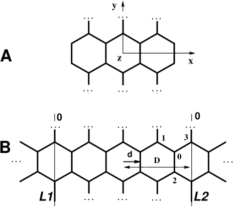
Figure 1: Boundary conditions for a 1D carbon ribbon (A) and the same ribbon placed in the graphene sheet (B). Carbon sites on lines $L_{1}$ and $L_{2}$ have zero coefficients of expansion.

The energy spectrum of nanographite materials (1D CRs, 1D CNTs, 0D RGM, 0D CNTs) can be obtained from the dispersion relation of graphene Wal :

$$\varepsilon_{+,-}=\varepsilon_{F}\pm\beta|\,e^{-iak_{y}\sqrt{3}/2}+2\cos ak_{x}/2|,$$ (1)

where $a=\sqrt{3}d_{CC}$, and $d_{CC}$ is the carbon-carbon distance. Here the $2\pi$ factor is incorporated in $k$, and $-\beta$ stands for the Hückel transfer integral (or $-t$ in the tight-binding model), so that $\beta>0$. At the $K-$point of the Brillouin zone of graphene two bands intersect:

$$ak_{x}^{K}=\pm\frac{4\pi}{3},$$ (2a)

$$ak_{y}^{K}=0.$$ (2b)

We start with studying energy spectrum of 1D CRs. The problem is how to reduce the problem to that for graphene. In the unit cell of a zigzag carbon ribbon there are four carbon atoms with 2 nearest neighbors while in graphene each carbon atom has 3 nearest neighbors, Fig. 1. Therefore, if we consider the ribbon as a part of the graphene 2D plane, Fig. 1B, the equations for the edge atoms of the ribbon are modified. For example, for site $0$ in Fig. 1B we have:

$$\frac{\varepsilon}{\beta}c_{0}=-(c_{1}+c_{2}+c_{3}),$$ (3)

where $c_{i}$, $i=0,1,2,3$ are coefficients of the expansion of graphene wave function $\psi_{g}$. However, if we put $c_{3}=0$, then Eq. (3) will be identical to that for the ribbon. Thus, we can select the solutions for the CR out of the graphene solutions by requiting $c_{j}=0$ for all carbon sites $j$ on lines $L_{1}$ and $L_{2}$ and by repeating the resulting pattern in the $x-$direction. The lines with $\psi_{r}=0$ completely separates neighboring nanoribbons from each other, since there is no interaction between them.

We arrive at the following conditions of quantization:

$$\cos(Dk^{\prime}_{x})=0,$$ (4a)

$$\sin(Dk^{\prime}_{x})=0.$$ (4b)

Here $D=md$ ($m$ is an integer) and $d=\sqrt{3}d_{CC}/2$. (Both distances are shown in Fig. 1B.) The number of carbon rings in the $x-$direction is ${\cal N}=m-1$. It is clear that the CR will be metallic if line $(k^{\prime}_{x},k^{\prime}_{y})$ in $k-$space goes through the $K-$point, Eqs. (2a), (2b). Solving Eqs. (4a), (4b) leads to

$$ak^{\prime}_{x}=2\pi\frac{n}{m},$$ (5)

where $n$ is an integer number. Condition (5) coincides with Eq. (2a), (2b) only if

$$m=3m^{\prime},$$ (6a)

$$n=2m^{\prime}.$$ (6b)

This immediately gives

$${\cal N}=3m^{\prime}-1.$$ (7)

Eq. (7) determines which CR is metallic. We get: ${\cal N}$=2, 5, 8,… . Substituting $(k^{\prime}_{x}=k_{x}^{K},k^{\prime}_{y}=k)$ in Eq. (1) leads to the dispersion relations for two bands which cross at the Fermi energy:

$$\varepsilon_{+,-}=\varepsilon_{F}\pm 2\beta\sin\frac{Xk}{4},$$ (8)

where $X=3d_{CC}$ ($X$ is the modulus of the basis vector in the $y-$direction). The corresponding density of states (DOS) per unit cell (for both spins projections) in the neighborhood of $\varepsilon_{F}=0$ is given by

$$\rho(\varepsilon)=\frac{2}{\pi}\,\frac{1}{\sqrt{1-(\varepsilon/2\beta)^{2}}}\,\frac{1}{\beta}.$$ (9)

Eq. (9) coincides with that for metallic CNTs Cha .

It is instructive to study the two electronic states at the Fermi energy, when $k_{F}=0$. We start by considering the simplest possible case: ${\cal N}=2$, Fig. 2. Then the following explicit eigenvectors can be found:

$$V_{1}=\frac{1}{2}\,\left\{0,-1,0,0,0,1,0,-1,0,1\right\},$$ (10a)

$$V_{2}=\frac{1}{2}\,\left\{-1,0,1,0,-1,0,1,0,0,0\right\}.$$ (10b)

$V_{1}$ is visualized in Fig. 1 by putting plus and minus signs at corresponding carbon sites. $V_{2}$ is obtained from $V_{1}$ through the mirror reflection at the $xz$ plane, which follows from the symmetry of the electronic system.

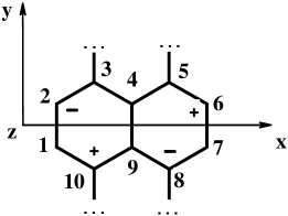
Figure 2: Unit cell of 1D metallic carbon ribbon. Plus signs (sites 6, 10) and minus signs (2, 8) refer to eigenvector $V_{1}$ at $\varepsilon_{F}=0$.

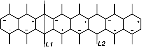
Figure 3: Unit cell of 1D metallic carbon ribbon containing 8 carbon rings. Plus and minus signs schematically indicate one of two eigenvectors at $\varepsilon_{F}=0$.

In this way one can construct two eigenvalues for any metallic CR. As an example in Fig. 3 we schematically draw one eigenvector for a CR with the 8 ring unit cell. Notice, that all three blocks have the structure of $V_{1}$, Fig. 2. The blocks are connected via chains of carbon sites - lines $L_{1}$ and $L_{2}$ - where $c_{j}=0$. As before, the second eigenvector is obtained from the first through the $xz-$mirror reflection. Thus, we can build two eigenvectors only if number of blocks is ${\cal N}=2+3n$, which also gives the rule (7).

From Eq. (1) one can derive the expression for energy gap $E_{g}$ if ${\cal N}\neq 3m^{\prime}-1$. There are two cases:(1) ${\cal N}=3m^{\prime}$ and $m=3m^{\prime}+1$, and (2) ${\cal N}=3m^{\prime}-2$, $m=3m^{\prime}-1$. In both cases the energy gap is given by

$$E_{g}=2\beta\,|1-\cos\frac{\delta\phi}{2}-\sqrt{3}\sin\frac{\delta\phi}{2}|,$$ (11a)

The value of $$\delta\phi K- n=2m^{\prime}$$ depends on which branch - Eq. (4a) or Eq. (4b) - is considered. [It is a measure of deviation from the point, Eq. (2a,b) in the zone-folding model.] For cos-like branches, Eq. (4a), we get , Eq. (6b), and

$$\delta\phi_{cos}=\mp\frac{\pi}{3({\cal N}+1)}.$$ (11b)

Here the first choice of $${\cal N} {\cal N}$$ corresponds to minus sign, while the second choice of to plus sign. For sin-like branches, Eq. (4a), we get

$$\delta\phi_{sin}=4\phi_{cos},\quad n=2m^{\prime}$$ (11c)

$$\delta\phi_{sin}=2\phi_{cos},\quad n=2m^{\prime}\pm 1$$ (11d)

By comparing Eq. (11b) with Eq. (11c) and Eq. (11d) we conclude that the gap is due to cos-like branches, Eq. (11b). If $\delta\phi_{cos}\ll 1$, which is often the case,

$$E_{g}=\beta\,\frac{4\pi}{\sqrt{3}}\frac{1}{{\cal N}+1}.$$ (12)

Thus, $E_{g}\sim 1/{\cal N}$ as it was the case for CNTs Cha .

The rule for the metallicity of armchair CRs, Eq. (7), is very different from the the rule for the corresponding zigzag CNTs characterized by the pair of indices $[{\cal N},0]$:

$${\cal N}=3m^{\prime}.$$ (13)

It is clear that the rules do not overlap meaning that if one rolls up a nanotube from a metallic ribbon, then the resultant nanotube will not be metallic and vice versa. This conclusion deserves a more detailed explanation. First, we notice that the metallicity rule for CNTs, Eq. (13), is obtained from the cyclic condition in the $x-$direction which allows for sin- and cos- like dependencies, while in case of ribbon only sin- like functions are allowed. [One can prove that Eq. (4a) does not include the $K-$point, Eq. (2a).] The sin-dependence in the $x-$direction implies opposite signs for coefficients $c_{j}$ belonging to edge sites $j$ on opposite sides of CR. By rolling up a nanotube the carbon sites on opposite edges of ribbon should coincide, which in turn destroys the odd solutions. The even solutions satisfying the cyclic condition survive the rolling up procedure but none of them has energy at $\varepsilon_{F}=0$.

We now turn to 0D objects - carbon macromolecules and nanotubes of finite length. Unlike 1D electron systems characterized by electron energy band structure, they have discrete energy spectra. However, these spectra are closely related with electron bands which we have already considered. In particular, energy levels of RGMs and CNTs near the Fermi energy are described by the following expression:

$$\varepsilon_{+,-}(n)=\pm 2\beta\sin\frac{Xk(n)}{4},$$ (14a)

where

$$k(n)=\delta k\,\left(n+\frac{1}{2}\right),$$ (14b)

$n=0,1,2$,… and $\delta k=\pi/L$, and $L=L_{0}+7d_{CC}/4$. Here $L_{0}$ is the length of nanotube or ribbon (maximal distance between carbon atoms in the $y-$direction, which has the armchair profile). We want to stress that Eqs. (14a), (14b) are exact, see Appendix. The electron spectrum given by (14a) is independent of width which is consistent with the situation observed for 1D objects. It is also worth noting that the spectrum of 0D carbon objects consists of many discrete levels and instead of Fermi level we should speak of highest occupied (HOMO) and lowest unoccupied (LUMO) molecular orbitals. This implies that formally we can not speak of metallicity and semiconductivity. However, in Tables 1-3 we retain these terms in a loose sense, because from one side, it shows relations with corresponding 1D objects and from the other side, the existence or nonexistence of a large energy gap at the HOMO-LUMO region remains one of the important characteristics of these systems.

Table 1: Length dependence of the energy spectrum of metallic RGMs (${\cal N}=2,5,...$) and CNTs (${\cal N}=3,6,...$).

	length, in $d_{CC}$
HOMO$-i$	299	149	29
1	-0.00783	-0.01563	-0.07661
2	-0.02350	-0.04689	-0.22937
3	-0.03917	-0.07813	-0.38078
4	-0.05483	-0.10935	-0.52996
5	-0.07049	-0.14055	-0.67603
6	-0.08615	-0.17172	-0.81814
7	-0.10180	-0.20284	-0.95544

Table 2: Length dependence of the energy spectrum of semiconducting RGM, ${\cal N}=10$. ($L_{0}=3.5d_{CC}$, $\delta=0.9$). “Exact” refers to the strait-forward Hückel calculations, “approx” to the values of Eq. (16a,b).

	299 $d_{CC}$		214 $d_{CC}$
HOMO$-i$	exact	approx.	exact	approx.
1	-0.08271	-0.08258	-0.08371	-0.08356
2	-0.08689	-0.08691	-0.09069	-0.09100
3	-0.09349	-0.09388	-0.10143	-0.10250
4	-0.10210	-0.10294	-0.11501	-0.11687
5	-0.11230	-0.11360	-0.13064	-0.13318
6	-0.12374	-0.12544	-0.14771	-0.15079
7	-0.13611	-0.13816	-0.16580	-0.16928

Table 3: Length dependence of the energy spectrum of semiconducting CNT $[10,0]$ (${\cal N}=10$, $L_{0}=3.75d_{CC}$, $\delta=0.9$). “Exact” refers to the strait-forward Hückel calculations, “approx” to the values of Eq. (16a,b).

	299 $d_{CC}$		214 $d_{CC}$
HOMO$-i$	exact	approx.	exact	approx.
1	-0.17634	-0.17623	-0.17691	-0.17673
2	-0.17864	-0.17847	-0.18088	-0.18067
3	-0.18241	-0.18226	-0.18733	-0.18723
4	-0.18756	-0.18750	-0.19602	-0.19615
5	-0.19400	-0.19406	-0.20671	-0.20712
6	-0.20161	-0.20182	-0.21910	-0.21982
7	-0.21027	-0.21065	-0.23296	-0.23398

It is clear that Eqs. (14a) and (14b) can be considered as a discretization of (8). Following this route we can derive an approximate expression for nonmetallic RGMs and CNTs. First, we recall that for 1D systems there are various bands, which we have discussed already while calculating $E_{g}$. In general their energy is

$$\frac{\varepsilon_{+,-}}{\beta}=\pm|e^{-i\frac{X}{2}k}-\cos\frac{\delta\phi}{2}-\sqrt{3}\sin\frac{\delta\phi}{2}|,$$ (15)

where $\delta\phi=\delta\phi_{sin}$ or $\delta\phi_{cos}$. The highest occupied band for RGMs is given by $\delta\phi_{cos}$, Eq. (11b). Starting with Eq. (15) and taking inspiration from the relation between (8) and (14a) we obtain the discretized version for $\varepsilon_{+,-}(n)$ of semiconducting RGMs or CNTs of finite length:

$$\frac{\varepsilon_{+,-}(n)}{\beta}=\pm|e^{-i\frac{X}{2}k^{\prime}(n)}-\cos\frac{\delta\phi}{2}-\sqrt{3}\sin\frac{\delta\phi}{2}|,\quad\quad$$ (16a)

$$k^{\prime}(n)=\delta k\,\left(n+\delta\right).$$ (16b)

Here $n=0,1,2$,… is integer, $\delta k=\pi/L$, and $L=L_{0}+\delta L$. In fact, in Eq. (16b) $\delta L\sim d_{CC}$ and $\delta\sim 1$ are phenomenological parameters which should be found by fitting a data set of $\varepsilon(n)$. The set can be taken from a Hückel calculation of RGMs and CNTs or even from a more advanced calculation (like density functional, for example). In Tables 2 and 3 we compare energy spectra given by Eq. (16a,b) [approx.] with straight-forward Hückel calculations [exact]. $\delta\phi$ in Eq. (16a) is $\phi_{cos}$, Eq. (11b), for graphene molecules, and

$$\delta\phi=\pm\frac{2\pi}{3{\cal N}}$$ (17)

in case of semiconductiong nanotubes with width ${\cal N}=3m^{\prime}\pm 1$. The accuracy of Eqs. (16a), (16b) is of the order of $10^{-3}\beta$ for 10 top occupied molecular orbitals (or HOMO$-i$, $i=1-10$), Tables 2, 3.

Finally, we remark on the doubly degenerate HOMO level at $\varepsilon\approx 0$ Nak ; Wak1 ; Wak2 . The nature of the states which are always present in the electronic spectrum of carbon ribbons and nanotubes of finite length, is an object of intense research Nak ; Wak1 ; Wak2 ; Mun ; Sas ; Son2 ; Hod . These states are edge ones, because as follows from Eqs. (14a), (14b) $\varepsilon_{HOMO-1}=-2\beta\sin(X\delta k/8)\neq 0$. The coefficients of the wave function expansion, $c_{j}$, in this case quickly fall to zero as we move away from the edges, and the states do not contribute to the conductivity in the $y-$direction, Fig. 1. To demonstrate it we have calculated the conductance of RGMs using the Landauer formula Imry . For a qualitative treatment, we define the self energy within the broadband approximation Muj , considering it as an energy-independent imaginary constant, $\Sigma=i\Delta$ ($\Delta=1$ eV). In Fig. 4 we plot conductance as a function of length at $\varepsilon_{F}=0$ for RGMs of various width. Our results show that metallic RGMs ($n=2,5,8$) have a weak dependence on length. Their conductances coincide starting with a rather short length of 2-6 rings. For other non-metallic RGMs the calculations demonstrate an exponential decrease of conductance with length. It is also worth noting that the conductance of metallic RGMs is always the same and equal to the conductance of the metallic RGM with the minimal width of 2 rings. (A detailed qualitative and quantitative analysis will be given elsewhere.)

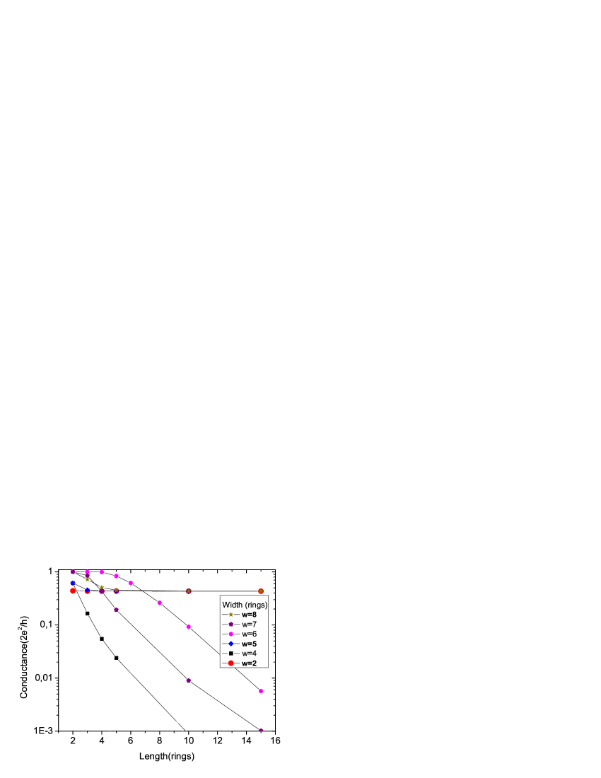
Figure 4: Conductance versus RGM length at $\varepsilon_{F}=0$.

In conclusion, we have studied the electronic spectrum of the 1D armchair CRs and zigzag CNTs and their 0D counterparts of finite length in the Hückel model. We have found the solutions by reducing the problem to that for graphene with appropriate selection rules imposed by boundary conditions. In the vicinity of the HOMO-LUMO energy region ($\varepsilon\sim 0$) we have found the exact expression for energy spectrum of metallic nanosystems, Eq. (14a,b) and approximate energy spectrum in case of semiconducting materials, Eq. (16a,b). Finally, we have calculated the conductance of some RGMs and investigated the role of edge states.

The authors would like to thank D. S. Kosov for helpful discussions.

APPENDIX

Here we discuss the derivation of Eq. (14a,b). For a 1D armchair CR or 1D zigzag CNT each of the discrete values of $k^{\prime}_{x}$ determines an electronic band. The metallic band is given by Eq. (2a) and obtained for the (4b) condition of quantization. This condition implies the $\sin[(2\pi/3)(x/d)]$ modulation in the $x-$direction with zero coefficients at $x/d=3l$ where $l=0,1,2,...$. (Distances and axes are shown in Fig. 1.) Each index $l$ defines a carbon ribbon in the $y-$direction with nonzero coefficients at $x_{1}/d=1+3l$ and $x_{2}/d=2+3l$. The lines with zero coefficients imply that each ribbon can be considered as independent. In fact, they are equivalent due to the modulation condition, Eq. (4b). We can use this property and work only with one ribbon shown in Fig. 5 and later reconstruct the solution for the whole system.

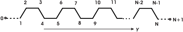
Figure 5: Effective 1D chain of $N$ carbon atoms [$i=1,2,...,N$] within the $l$-ribbon. Also shown are two auxiliary carbon atoms [$i=0$ and $i=(N+1)$], see text for details.

Now we consider one ribbon in the $y-$direction which is equivalent to a one dimensional (1D) chain of carbon atoms ($i=1,2,...,N$). Considering a solution with the coefficients $c_{j}$ of the wave function expansion, we obtain for them the following relations

$$\frac{\epsilon}{\beta}c_{j}=-(c_{j-1}+c_{j+1}),$$ (A-1)

where $j=2,3,...,(N-1)$. The problem arises due to the two boundary atoms: $j=1$ and $j=N$. To solve this task we will use the trick which we have already applied to 1D ribbon with Eq. (3). That is, we introduce two auxiliary carbon atoms $j_{b1}=0$ and $j_{2b}=(N+1)$ and consider an infinite 1D carbon chain beyond them. Notice, that for the following the real shape of the 1D chain is immaterial, it can be equally thought of as a 1D linear chain of carbon atoms. For an infinite chain the general solution is $c_{j}\sim exp(-\phi^{\prime}\,j)$, where $\phi^{\prime}=d_{CC}\,k^{\prime}_{y}$ and $k^{\prime}_{y}$ is an effective wave number. Then the coefficients at $j_{b}$ should be zero, i.e. $c_{0}=c_{N+1}=0$. This gives a condition of quantization,

$$\sin(L_{y}\,k^{\prime}_{y})=0,$$ (A-2)

where $L_{y}=(N+1)\,d_{cc}$. From (A-2) we get

$$k^{\prime}_{y}=\frac{\pi}{L_{y}}\,r=\frac{\pi}{(N+1)\,d_{CC}}\,r.$$ (A-3)

Here positive integer $r=1,2,...,N$. The energy of the 1D chain is obtained from Eq. (A-1):

$$\epsilon/\beta=-2\cos(\phi^{\prime})=-2\sin\left(\frac{\pi}{2}-\phi^{\prime}\right).$$ (A-4)

The latter relation can be written as

$$\epsilon/\beta=-2\sin\left(\frac{\pi}{N+1}(n+\frac{1}{2})\right),$$ (A-5)

where

$$2n=N-2r.$$ (A-6)

Notice that $n=N/2-1$, $(N/2-2)$, …, $-N/2$. ($N$ is even, because $N=4N_{hex}$, where $N_{hex}$ is the number of hexagons in the $y-$direction.) First $N/2$ electron states are occupied by $N$ $\pi$-electrons. Taking into account that the length of CR or CNT in the $y-$direction,

$$L_{0}=\left(\frac{3}{4}N-1\right)\,d_{CC},$$ (A-7)

Eq. (A-5) can be rewritten as

$$\epsilon/\beta=\mp 2\sin\left(\frac{3d_{CC}}{4}\frac{\pi}{(L_{0}+7d_{CC}/4)}(n^{\prime}+\frac{1}{2})\right),$$ (A-8)

where the solution with the minus sign refers to the occupied states at the Fermi level: HOMO ($n^{\prime}=0$), and the HOMO$-n^{\prime}$ levels ($n^{\prime}=1,2,...,N/2$.) The solution with the plus sign refers to the unoccupied states: LUMO ($n^{\prime}=0$), and the LUMO$+n^{\prime}$ levels ($n^{\prime}=1,2,...,N/2$.). Eq. (A-8) is equivalent to Eq. (14a,b). Finally, we would like to notice that the equation implies a certain size relation of RGM, $L_{y}=L_{0}>L_{x}$. The latter condition is needed to assure that a set of levels around the Fermi level is associated with a 1D metal band and separated from other $k^{\prime}_{x}-$levels (other 1D bands). If it is not so ($L_{y}=L_{0}<L_{x}$) then the levels described by (A-8) do exist but they are not grouped together. They are mixed up with other $k^{\prime}_{x}-$levels.

References

- (1) S. Iijima, Nature 354, 56 (1991).
- (2) M. S. Dresselhaus, G. Dresselhaus, and P. C. Eklund, Science of Fullerenes and Carbon Nanotubes (Academic Press, San Diego, 1996).
- (3) R. Saito, G. Dresselhaus, and M. S. Dresselhaus, Physical Properties of Carbon Nanotubes (Imperial Colledge Press, London, 1998).
- (4) K. S. Novoselov, Z. Jiang, Y. Zhang, S. V. Morozov, H. L. Stormer, U. Zeitler, J. C. Maan, G. S. Boebinger, P. Kim, and A. K. Geim, Science 315, 1379 (2007).
- (5) A. Geim and K. Novoselov, Nat. Mater. 6, 183 (2007).
- (6) K. Nakada, M. Fujita, G. Dresselhaus, M.S. Dresselhaus, Phys. Rev. B 54, 17954 (1996).
- (7) M. Y. Han, B. Özyilmaz, Y. Zhang, P. Kim, Phys. Rev. Lett. 98, 206805 (2007).
- (8) B. Özyilmaz, P. Jarillo-Herrero, D. Efetov, D. A. Abanin, L. S. Levitov, P. Kim, Phys. Rev. Lett. 99, 166804 (2007).
- (9) H. Zheng, Z.F. Wang, T. Luo, Q. W. Shi, J. Chen, Phys. Rev. B 75, 165414 (2007).
- (10) H. Raza and E. C. Kan, Phys Rev. B 77, 245434 (2008).
- (11) J. Scott-Bunch, Y. Yaish, M. Brink, K. Bolotin, P. L. McEuen, Nano Lett. 5, 287 (2005).
- (12) K. S. Novoselov, A. K. Geim, S. V. Morozov, D. Jiang, Y. Zhang, S. V. Dubonos, I. V. Grigorieva, and A. A. Firsov, Science 306, 666 (2004).
- (13) J.-C. Charlier, X. Blase, S. Roche, Rev. Mod. Phys. 79, 677 (2007).
- (14) L. Malysheva and A. Onipko, Phys. Rev. Lett. 100, 186806 (2008).
- (15) K. Wakabayashi, M. Fujita, H. Ajiki, M. Sigrist, Phys. Rev. B 59, 8271 (1999).
- (16) Y.-W. Son, M. L. Cohen, S. G. Louie, Phys. Rev. Lett. 97, 216803 (2006).
- (17) V. Barone, O. Hod, G. E. Scuseria, Nano Lett. 6, 2748 (2006).
- (18) C. T. White, J. Li, D. Gunlycke, J. W. Mintmire, Nano Lett. 7, 825 (2007).
- (19) M. Fujita, K. Wakabayashi, K. Nakada, K. Kusakabe, J. Phys. Soc. Jpn. 65, 1920 (1996).
- (20) P. R. Wallace, Phys. Rev. 71, 622 (1947).
- (21) F. Munoz-Rojas, D. Jacob, F. Fernandez-Rossier, J. J. Palacios, Phys. Rev. B 74, 195417 (2006).
- (22) K. Sasaki, S. Murakami, R. Saito, Appl. Phys. Lett. 88, 113110 (2006).
- (23) Y.-W. Son, M. L. Cohen, S. G. Louie, Nature 444, 347 (2006).
- (24) O. Hod, V. Barone, G. E. Scuseria, Phys. Rev. B 77, 035411 (2008).
- (25) Y. Imry and R. Landauer, Rev. Mod. Phys. 71, 306 (1999).
- (26) V. Mujica, M. Kemp, M. A. Ratner, J. Chem. Phys. 101, 6856 (1994).