EXCESS SPECIFIC HEAT OF PTFE AND PCTFE AT LOW TEMPERATURES: APPROXIMATION DETAILS

Nina B. Bogdanova$\,{}^{a)}$, B.M. Terziyska$\,{}^{b)}$

$\,{}^{a)}$Inst.of Nuclear Research,BAS, 72 Tzarigradsko choussee, 1784 Sofia, Bulgaria, Email:nibogd@inrne.bas.bg
$\,{}^{b)}$Inst.of Solid State Physics,BAS, 72 Tzarigradsko choussee, 1784 Sofia, Bulgaria, Email:terzyska@issp.bas.bg

Abstract

Approximation of the previously estimated excess specific heat $C^{excess}/T^{5}$ of two fluoropolymers, $PTFE$ and $PCTFE$, is presented using Orthonormal Polynomial Expansion Method (OPEM). The new type of weighting functions in OPEM involves the experimental errors in every point of the studied thermal characteristic. The investigated temperature dependence of the function $C^{excess}/T^{5}$ is described in the whole temperature ranges $0.4\div 8K$ and $2.5\div 7K$ respectively for PTFE and PCTFE as well as in two subintervals $(0.4\div 2)K$, $(2.5\div 8)K$ for PTFE. Numerical results of the deviations between the evaluated $C^{excess}/T^{5}$ data and their approximating values are given. The usual polynomial coefficients obtained by orthonormal ones in our OPEM approach and the calculated in every point absolute, relative and specific sensitivities of the studied thermal characteristic are proposed too. The approximation parameters of this type thermal characteristic are shown in Figures and Tables.

Key words: orthonormal and usual polynomial approximation, low-temperature excess specific heat of two fluoropolymers - PTFE and PCTFE

I.INTRODUCTION

The unusual thermal properties concerning the low-temperature specific features of the heat capacities of the polytetrafluoroethylene (PTFE) and polyclorothrifluoroethylene (PCTFE) were considered in an earlier paper [1]. The estimated there excess specific heat over Debye contribution below 10 K of these fluoroplasts was discussed in the frame of the recently developed Soft-Potential Model (SPM).
The present study is devoted to the mathematical description of the low-temperature excess specific heat of these semi-crystalline polymers applying Orthonormal Polynomial Expansion Method (OPEM) [2].

II.EXCESS SPECIFIC HEAT DATA

The previous work [1] clarifies several points concerning the specific heat peculiarities observed in $C_{p}/T^{3}$ temperature dependencies of PTFE and PCTFE, a maximum appearing around $T_{max}$= 4 K for both polymers and a found shallow minimum for PTFE centered at $T_{min}=1~{}K$. Following the Soft-Potential Model (SPM) [3, 4, 5, 6], supposing a coexistence of acoustic phonons with quasi-localized low-frequency (soft) modes in glasses and successfully applied by us to some chalcogenide glasses [7, 8], the specific heat data, taken from the available calorimetric measurements at low-temperatures ($T~{}<10$ K) for the studied fluoroplasts [9, 10], were described in a paper [1]. The $C_{p}$ components are:
i) $C_{p}^{TLS}$ - a linear contribution, described by double-well potentials, conditioned by the thermal exitations of the tunneling state (TLS); for PTFE it was established to predominate at $T~{}\leq 0.2~{}K$.
ii) $(C_{p}^{D})^{acou}$ - a cubic Debye contribution, evaluated and discussed in details in a paper [1].
iii) $C_{p}^{exc(SM)}$ - an excess specific heat (a soft mode) contribution of the quasi-harmonic exitations, described by single-well potentials.
$C_{p}^{exc(SM)}$ component was evaluated [1] by difference between the measured specific heat $C_{p}$ [9, 10] and the sum ($C_{p}^{TLS}$ + $(C_{p}^{D})^{acou}$) as follows.

$$C_{p}^{exc(SM)}=C_{p}-[C_{p}^{TLS}+(C_{p}^{D})^{acou}],$$ (1)

The temperature dependencies of the three specific heat components in Eq. 1 are:

$$C_{p}^{TLS}=C_{TLS}T,\hskip 8.5359ptC_{p}^{D}=(C_{D})^{acou}T^{3},\hskip 8.5359ptC_{p}^{exc}=C^{exc(SM)}T^{5}.$$ (2)

The abbreviations of Two Level State, Debye and excess specific heat (Soft Modes) are marked with $TLS$, $D$, and $exc(SM)$, respectively. Here, $C_{TLS}$ was determined by the $C_{p}$ experimental data of Nittke et al [9]; $(C_{D})^{acou},$ the true elastic coefficient, was calculated [1] by the macroscopic parameters of the investigated materials and the average sound velocity $v_{s}$, evaluated [1] for PTFE (PCTFE) by available measurements of transversely and longitudinally polarized 10 (5) MHz ordinary sound waves between 4.2 and 140 (180) K. Note that the average sound velocity $v_{s}$ for both polymers changes its value about 0.3 % within 0 and 10 K. This fact allows us to accept up to 10 K a constant Debye coefficient of the Debye specific heat contribution by acoustic measurements .
The quantities $C_{D}$ up to 10 K and $C_{TLS}$ are independent of the temperature. In accordance with the SPM, the softening of the lattice vibrations leads to increasing of the density of states of the harmonic oscillators with rising of their energy $E$. This increase appears to be proportional to the energy as $E^{4}$ leading to proportional to $T^{5}$ term in $C_{p}(T)$ at enough low-temperatures, i.e. the quantity $C^{exc(SM)}$ is temperature independent only in a narrow low-temperature range, $0<T<1.5T_{min}$. It is worth to mention that the quantity $C^{exc(SM)}$ evaluated for some glasses [11, 12, 13] confirms this prediction of the SPM. For the studied polymers [1] $T_{min}$ was estimated to be very close to 1 K. But in wider low-temperature range the temperature dependencies of the quantities $C_{p}^{exc(SM)}/T^{5}$ and the excess specific heat $C_{p}^{exc(SM)}$ presented, respectively in Fig.1 and in the inset of the Fig.1, are temperature dependent. As it can be seen in the inset of Fig.1, the Soft Modes (SM) delocalized at T = 8 K for PTFE and at T = 7 K for PCTFE.

Figure 1: Temperature dependencies of the excess specific heat presented as $C^{exc}/T^{5}$; inset: Temperature dependencies of the excess specific heat $C^{exc}$ $[mJ/gK]$ of the PTFE and PCTFE

.

It is important to note that $C^{exc}/T^{5}$ function changes its temperature behavior just at $T=(3/2)T_{min}$.

III. MATHEMATICAL APPROACH

Our Orthonormal Polynomial Expansion Method(OPEM) and its applications in cryogenic thermometry are presented in papers [2, 14, 15, 16]. Some important features of OPEM concerning cryogenic thermometry at the approximation of thermometric characteristics of different type low- temperature sensors are protected by a patent for an invention [15]. Our OPEM is defined on Forsythe [16] three-term relation for constructing orthogonal polynomials over discrete point set with arbitrary weights in the term of the least square method. The one-dimensional recurrence for generation of orthonormal polynomials $\{\Psi_{k}^{(0)}$, $k=1,2,\ldots\}$ and their derivatives $\{\Psi_{k}^{(m)},m=0,1,2,\ldots\}$, in OPEM is:

$$\Psi_{k+1}^{(m)}(q)=\gamma_{k+1}[(q-\alpha_{k+1})\Psi_{k}^{(m)}(q)-\\ (1-\delta_{k0})\beta_{k}\Psi_{k-1}^{(m)}(q)+m\Psi_{k}^{(m-1)}(q)]$$

OPEM is a development of the Forsythe approach for receiving derivatives and integrals with fourth term in the Eq. (3). The polynomials $\{\Psi_{k}^{(0)}\}$ satisfy the orthogonality relations:

$$\sum_{i=1}^{M}w_{i}\Psi_{k}^{(0)}(q_{i})\Psi_{l}^{(0)}(q_{i})=\delta_{kl}$$

over the point set $\{q_{i},i=1,2,\ldots M\}$ with weights $w_{i}=1/\sigma_{i}^{2}$ , depending on errors $\sigma_{i}$ in every point. The approximating values $f^{appr}$ of the function and its $m$-th derivative $f^{(m)appr}$,$\{m=0,1,..\}$ are calculated by

$$f^{(m)appr}(q)=\sum_{k=0}^{N}a_{k}\Psi_{k}^{(m)}(q)=\sum_{k=0}^{N}c_{k}q^{k}.$$ (3)

The optimal degree $N$ of the approximating polynomials in Eq.(4) is selected by the algorithm, combining the following two criteria. First, the fitting curve should lie in the error corridor of the dependent variable $(q_{j},f_{j}^{exp}\pm{\sigma_{j}},j=1,...M)$.

$$(f_{j}^{appr}-f_{j}^{exp})^{2}w_{j}\leq{1}.$$ (4)

Second, the minimum $\chi^{2}$ should be reached.

$$\sum_{j=1}^{M}{w_{j}(f_{j}^{appr}-f_{j}^{exp})^{2}}/(M-N-1)\rightarrow{min}.$$ (5)

When the first criterion is satisfied, the search of the minimum $\chi^{2}$ stops. The development of the algorithm in the biophysics with the total variance formula for involving the errors in independent variable was published in a paper [17]. The last version with obtaining of usual $c_{k}$ coefficients from orthogonal ones $a_{k}$ from Eq. 3 is developed in our work, RSI-2005 [2].

IV. APPROXIMATION RESULTS
A. Orthonormal expansion

The temperature dependence of the $C^{exc}/T^{5}$ function is described by orthonormal polynomials in the whole temperature range $0.4\div 8$ $[K]$ or in two subintervals $0.4\div 2$  $[K]$, $2.5\div 8$ $[K]$ for PTFE, and in the temperature range $2.5\div 7$  $[K]$ for PCTFE, using the new type of weights, $W^{C^{exc}/T^{5}}$. The studied thermal characteristic $C^{exc}/T^{5}$ and its sensitivities, absolute $d(C^{exc}/T^{5})/dT$, relative $[1/(C^{exc}/T^{5})]d(C^{exc}/T^{5})/dT$ and specific, $[T/(C^{exc}/T^{5})]d(C^{exc}/T^{5})/dT$, evaluated in every point, are shown in linear-linear plot in Figs.2 and 3 for PTFE and PCTFE, respectively. It is worth to note that the subintervals for PTFE are chosen by the temperature behavior of the specific sensitivity of this polymer (see Fig.2).

Figure 2: Temperature dependencies of the relative $[1/(C^{exc}/T^{5})]d(C^{exc}/T^{5})/dT$ $[K^{-1}]$ and specific $[T/(C^{exc}/T^{5})]d(C^{exc}/T^{5})/dT$ $[-]$ sensitivities of the PTFE; inset: Temperature dependencies of the absolute sensitivity $d(C^{exc}/T^{5})/dT$.

Figure 3: Temperature dependencies of the relative $[1/(C^{exc}/T^{5})]d(C^{exc}/T^{5})/dT$ $[K^{-1}]$ and specific $[T/(C^{exc}/T^{5})]d(C^{exc}/T^{5})/dT$ $[-]$ sensitivities of the PCTFE; inset: Temperature dependencies of the absolute sensitivity $d(C^{exc}/T^{5})/dT$ $[mJ/gK^{7}]$.

By definition the weighting function $W^{C^{exc}/T^{5}}$ is $1/\sigma^{2}$, where $\sigma^{2}$ is a variance of the thermal characteristic $C^{exc}/T^{5}$ versus temperature $T$. In our investigation this variance is accepted to be, correspondingly square of the absolute heat capacity resolution $\Delta C^{exc}_{acr}$, determined by the experimental specific heat accuracy as follows: $(\Delta C^{exc}_{acr})_{i}=0.025(C^{exc}/T^{5})_{i}$  $[mJ/gK^{6}]$ for the first approximating interval of PTFE and $(\Delta C^{exc}_{acr})_{i}=0.1(C^{exc}/T^{5})_{i}$  $[mJ/gK^{6}]$ for both, the whole PCTFE approximating interval and the second approximating interval of PTFE. Here the weights, $W^{C^{exc}/T^{5}}$ are expressed by the relations:

$$(W^{C^{exc}/T^{5}})_{i}=1/(\Delta C^{exc}/T^{5}_{acr})_{i}=1600/(C^{exc}/T^{5})^{2}_{i}~{}~{}[mJ/gK^{6}]^{-2}$$ (6)

for the first approximating interval of PTFE, or

$$(W^{C^{exc}/T^{5}})_{i}=1/(\Delta C^{exc}_{acr})_{i}=100/(C^{exc}/T^{5})^{2}_{i}~{}~{}[mJ/gK^{6}]^{-2}$$ (7)

for the PCTFE and the second approximating interval of PTFE. The deviations $\Delta(C^{exc}/T^{5})_{i}$ between experimental and approximating values of the excess specific heat are estimated in every point by the expression:

$$\Delta(C^{exc}/T^{5})_{i}=(C^{exc}/T^{5})_{i}^{exp}-(C^{exc}/T^{5})_{i}^{appr}$$ (8)

The temperature behavior of the calculated differences $\Delta(C^{exc}/T^{5})_{i}$, the root mean square deviations $RMS^{C}$ and the mean absolute deviations $MAD^{C}$ respectively for PTFE and PCTFE excess specific heat approximations are shown in the Figs.4,5 and 6.

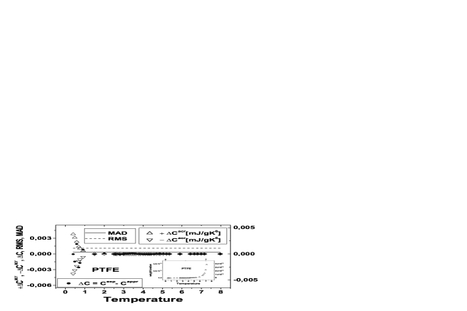
Figure 4: Temperature dependencies of $\Delta(C^{exc}/T^{5})$, $(\Delta(C^{exc}/T^{5})_{acr}$, $MAD^{C^{exc}/T^{5}}$ and $RMS^{C^{exc}/T^{5}}$ of the PTFE for the whole approximated temperature range;inset:Temperature dependence of the weighting function $w(T)$ for FTPE .

Figure 5: Temperature dependencies of $\Delta(C^{exc}/T^{5})$, $(\Delta(C^{exc}/T^{5})_{acr}$, $MAD^{C^{exc}/T^{5}}$ and $RMS^{C^{exc}/T^{5}}$ of the PTFE for two interval approximation.

Figure 6: Temperature dependencies of $\Delta(C^{exc}/T^{5})$, $\Delta(C^{exc})_{acr}$, $MAD^{C^{exc}/T^{5}}$ and $RMS^{C^{exc}/T^{5}}$ of the PCTFE for the whole approximated temperature range.

The RMS deviation is more popular. It is given in another our paper [2]. The characteristics MAD is defined as follows:

$$MAD^{C}=\frac{1}{M}\sum_{i}|{\Delta(C^{exc}/T^{5})_{i}-\overline{\Delta(C^{exc}/T^{5})}|},$$ (9)

where $\overline{\Delta(C^{exc}/T^{5})}=\frac{1}{M}\sum_{i}{\Delta(C^{exc}/T^{5})_{i}}$ and $\Delta(C^{exc}/T^{5})_{i}$ are calculated from Eq.(9).
Following the cited criteria in Eqs.(5,6) the deviations $\Delta(C^{exc}/T^{5})_{i}$ are in the error corridor (see Eq.5). As a result of our approximation, the polynomial degree for temperature range of PTFE subintervals is lower than for the whole temperature range. For $C^{exc}/T^{5}$ vs. $T$ approximation the optimal degree $N$ as well as some main characteristics including the overall approximation characteristics: RMS and MAD of $\Delta C^{exc}/T^{5}$ vs. $T$ approximation, the weighting function $W^{C}$ and a goodness of fit $\chi^{2}$ are presented in the  TABLE 1.

B.Usual expansion obtained by orhonormal one

The next step in our approximation is done here. The OPEM is extended by calculation of usual coefficients $\{{c}_{k}\}$ from orthonormal ones $\{{a}_{k}\}$ using Eq.(4). This is carried out for the investigated intervals. The calculations are made for the $C^{exc}/T^{5}=f(T)$ descriptions, in two runs: first - in an interval [-1,1], and second - in the input intervals. Optimal values of usual polynomial degrees are chosen using two new criteria.

Table 1: OPEM approximations of $C^{excess}/T^{5}$ for $PTFE$ and $PCTFE$

T	C	N	$W^{C}$	$RMS^{C}$	$MAD^{C}$	$\chi^{2}$
$[K]$	$[\mu J/gK^{6}]$	-	$[mJ/gK^{6}]$	$[mJ/gK^{6}]$	-
$0.4\div 2$	$152\div 1$	6	$6.91\times{10}^{4}\div 1.60\times{10}^{9}$	$0.121\times 10^{-2}$	$0.828\times 10^{-3}$	1.38
$2.5\div 8$	$1\div 0.015$	4	$2.65\times 10^{8}\div 4.44\times 10^{11}$	$0.265\times 10^{-4}$	$0.208\times 10^{-4}$	0.57
$0.4\div 8$	$152\div 0.015$	8	$6.91\times 10^{4}\div 4.44\times 10^{11}$	$0.109\times 10^{-2}$	$0.326\times 10^{-3}$	0.95
$2.5\div 7$	$1.75\div 0.031$	6	$3.26\times 10^{7}\div 1.04\times 10^{11}$	$0.428\times 10^{-4}$	$0.306\times 10^{-4}$	0.58

Table 2: Usual coefficients for $C^{excess}/T^{5}$ $[10^{-3}mJ/gK^{6}]$ vs. $T$ approximation

$material$	$PTFE$			$PCTFE$
$RangeT(K)$	$0.4\div 2$	$2.5\div 8$	$0.4\div 8$	$2.5\div 7$
$Range(C^{exc.}/T^{5})$	$152\div 1$	$1\div 0.015$	$152\div 0.015$	$1.75\div 0.031$
$c_{0}$	.022854	.003118	.016067	.182459
$c_{1}$	-.001420	-.009158	-.063937	-.667996
$c_{2}$	.105876	.011825	.103755	.997805
$c_{3}$	-.582978	-.006389	-.070355	-.769121
$c_{4}$	-.390617	.001190	-.008661	.320591
$c_{5}$	.845833	-	.048421	-.068068
$c_{6}$	.696453	-	-.033867	.005687
$c_{7}$	-	-	.010411	-
$c_{8}$	-	-	-.001230	-

The first criterion is:

$$\max|f_{i}^{exp}-f_{i}^{appr,u}|/f_{i}^{exp}\rightarrow{min},$$ (10)

where $f^{appr,u}$ is the approximating function defined with usual expansion. The second criterion is:

$$\Delta\{c_{k}\}_{1}^{N}\rightarrow{min},$$ (11)

where $\{\Delta c_{k}\}$ are inherited errors in usual coefficients, defined in OPEM, discussed in a paper[18]. In the TABLE 2 the usual coefficients for $C^{exc}/T^{5}$ vs. $T$ approximation are presented.

In conclusion, the heat capacity components of the studied fluoroplasts are well defined earlier [1] using the SPM. In this study, the temperature dependencies of the excess specific heat of PTFE and PCTFE below 10 K presented as $C^{exc(SM)}/T^{5}$ are described by an Orthonormal Polynomial Expansion Method (OPEM). An approximation of the above mentioned thermal characteristic by usual polynomials, obtained by orthonormal ones, is given too. The numerical results for approximation characteristics as root mean square deviation, mean absolute deviation and normalized $\chi$ square assure good accuracy for calculated values of physical quantity in the input temperature intervals. Our approach for description of this characteristic proposes possibility for the future analyzing the low-temperature excess specific heat of the materials with glass-like behavior.

References

• [1] B. Terziyska, H. Madge, Some special feature of low-temperature specific heat of PTFE and PCTFE analyzed within the Soft Potential Model, to be published.
• [2] N.Bogdanova, B. Terzijska, Thermometric characteristics approximation of Germanium film temperature microsensors by orthonormal polynomials, Rev. Sci. Instrum. 68 (10), 3766-3771 (2005).
• [3] M.A.Il’in, Karpov V.G., and Parshin D.A., Parameters of soft atomic potentials in glasses, Zh. Exper. Teor. Fiz. 92, 291 (1987).
• [4] V.G.Karpov , Klinger M.I., and Ignat’ev F.N., Theory of low-temperature anomalies in the thermal properties of amorphic structures, Zh. Exper. Teor. Fiz. 84 (2), 760-775 (1983).
• [5] D.A.Parshin, Interactions of soft atomic potentials and universality of low- temperature properties of glasses, Phys. Rev. B 49 (14), 9400-9418 (1994).
• [6] D.A.Parshin, Liu X., Brand O., and Lohneysen H.v., Analysis of the low-temperature specific heat of amorphous AsxSe1-x within the soft potential model, Z. Phys. B 93 (1), 57-62 (1993).
• [7] B. Terziyska, H. Misiorek, E. Vateva, A. Jezovski, and D.Arsova, Low-temperature thermal conductivity of GexAs40-xS60 glasses, SSC 134, 349 (2005).
• [8] B. Terziyska, A. Czopnik, E. Vateva, D. Arsova, and R. Czopnik, Low-temperature specific heat of Ge-As-S glasses, Phil. Mag. Letters, 85, 145-150 (2005).
• [9] A. Nittke, P. Esquinazi, H.C. Semmelhack, A.L. Burin, A.Z. Patashinskii, Eur. Phys. J. B8, 19 (1999).
• [10] B. Terziyska, H. Madge, and V. Lovtchinov, Specific heat of PTFE and PCTFE within the temperatute range 2.5-20 K, Journal of Thermal Analysis 20, 33 (1981).
• [11] M.A.Ramos, Talon C, and Vieira S.,The Boson peak in structural and oriental glasses of simple alcohols: specific heat at low temperatures, J. Non-Cryst. Sol. 307-310, 80-86 (2002) and references therein.
• [12] C.Talon , Ramos M.A., and Vieira S.,Low-temperature specific heat of amorphous, orientational glass, and crystal phases of ethanol, Physical Review B 66, 012201(4)(2002).
• [13] M.A.Ramos, Talon C., Jimenez-Rioboo RJ, and Vieira S. Low-temperature specific heat of structural and orientational glasses of simple alcohols, J. Phys.:Condens. Matter 15, S1007-S1018 (2003).
• [14] N.Bogdanova, B. Terzijska, A novel approach to the Rh-Fe thermometric characteristic approximation,Β Commun. JINR, Dubna, E11–97-396 (1997).
• [15] B. Terzijska, N.Bogdanova, Weighted Orthonormal Polynomial Method in Cryogenic Thermometry, A Patent for an Invention, Bulgaria, No. 62582 (2000).
• [16] G.Forsythe, Generation and Use of Orthogonal Polynomials, J. Soc. Ind. Appl. Math. 5, 74-88 (1957).
• [17] N.Bogdanova, S. Todorov, Fitting of water Hydrogen bond energy data with uncertainties in both variables by help of orthogonal polynomials, Int. J. Modern Physics C 12, 1 (2001).
• [18] N.Bogdanova, Orthonormal Polynomial Expansion Method with errors in variables, E11-98-3,Β Communication JINR, Dubna (1998).