Simulating weak lensing on CMB maps

Abstract

We present a fast, arbitrarily accurate method to simulate the effect of gravitational lensing of the Cosmic Microwave Background anisotropies and polarization fields by large scale structures. We demonstrate the efficiency and accuracy of the method and exhibit their dependence on the algorithm parameters.

I Introduction

Weak lensing effects on the Cosmic Microwave Background (CMB) temperature and polarization anisotropies has been proposed as a probe of the total matter distribution in Large Scale Structures (LSS) between us and the surface of last scattering blanchard1987 ; seljak1998 ; zaldarriaga1998 ; hu1999a ; hu1999b ; zaldarriaga1999 ; guzik2000 ; waerbeke2000 ; benabed2001 ; hu2000 ; kesden2002 ; hirata2003b ; hirata2003a ; kesden2003 ; hirata2004 ; lewis2005 ; challinor2005 ; lewis2006 ; smith2007 . Although sensitive to the cumulative distribution of matter, it is quite complementary to the other probes of the matter distribution of the LSS. Indeed, it does not suffer from bias effects (as e.g. galaxy redshift surveys, Lyman-$\alpha$ forest), or from possible mis-determination of the redshift sources (cosmic shear measurements on galaxies). In addition, due to the high redshift of the source (last scattering surface) and the lensing efficiency function, weak lensing of CMB anisotropies is mostly sensitive to large scale structures which are still (mainly) in the linear regime, which makes it a very useful tool for cosmology, in particular to constrain the properties of neutrinos perotto2006 ; lesgourgues2006 .

Unlike shear measurements on galaxies, where the (reduced) shear field is directly sampled via measurement of galaxy ellipticities, measuring weak lensing effects on the CMB is complicated by the fact that the source itself can only be modeled by a stochastic realization of a field. However, theoretical arguments lead us to think that CMB anisotropies are highly Gaussian guth1981 ; linde1982 ; albrecht1982 , which has been confirmed on the data, at large scales, using different non-Gaussianity estimators (pdf, bispectrum, wavelet skewness and kurtosis, Minkowski functionals, etc.). These properties of the CMB anisotropies can be used to disentangle to some extent the stochastic properties of the (unlensed) CMB anisotropies from the stochastic properties of the lens (i.e. the LSS) as the lensing effect induces small specific non-Gaussian features in the CMB maps: it locally correlates the anisotropies with their gradient seljak1998 ; cooray2001a ; cooray2001b ; cooray2001c ; cooray2002 which in turn has lead to the development of specific estimators of the lensing potential field and its power spectrum hu2002 ; hirata2003b ; hirata2003a ; okamoto2003 .

Recently, weak lensing of the CMB anisotropies by LSS has been measured on WMAP data smith2007 by cross-correlation with a high-redshift radio galaxy catalog. Although marginally detectable in WMAP data due to its noise level, CMB lensing should be measured with high signal to noise by Planck with temperature anisotropies hu2002 ; hu2004 without needing to rely on an external data set. However, in order to carry out such a measurement on realistic CMB data, the impact of instrumental (anisotropic beams, missing data, correlated noise) and astrophysical (Galaxy contamination, point sources, etc.) systematic effects on the CMB lensing estimators has to be studied with great care.

The power spectra (temperature, and polarization) can be computed, using simple Taylor expansion at large scales hu2000 , or a more clever resummation scheme at smaller scales where the displacement field amplitude is comparable to the wavelength of the anisotropies challinor2005 . For smaller scales, or to investigate the different systematics described above, the development of fast and accurate methods to simulate the lensed CMB maps are needed.

This simulation is two-fold. On one hand, an accurate simulation of the large scale structure induced lensing deflection field is needed. On the other hand, one needs a method to apply this deflection field to an unlensed, simulated, CMB. We will not consider the first part of this program. Indeed, approximating the lensing effect with a single lens plane in the so-called Born approximation hu2000 has been shown to be an excellent approximation, both for temperature and polarization anisotropies. In this case, the simulation of lensed CMB maps reduces to an accurate resampling of the unlensed anisotropies at displaced positions. To solve this last problem, several technical solutions have been implemented. In the publicly distributed Lenspix code lenspix , different possibilities are available, namely:

• brute-force resampling by direct resummation of spherical harmonics at displaced positions (slow, but very accurate, this option should be considered as the “benchmark” for all other resampling methods)

• resampling on locally Cartesian grids with subsequent polynomial interpolation

For the last option, an interesting speed-up has been proposed by Hirata hirata2004 ; das_bode2008 by noting that a band-limited signal in spherical harmonics can be recast as a band-limited signal in regular Fourier modes on a $(\theta,\varphi)$, thus allowing a fast resampling of the signal on a Cartesian $(\theta,\varphi)$ grid using 2D FFTs.

In this paper, we investigate a variation on Hirata’s idea hirata2004 ; das_bode2008 , where the oversampling plus polynomial interpolation is replaced by an approximate (but arbitrarily accurate) Fast Fourier Transform (FFT) resampling on irregularly spaced grid points nfft .

The rest of this paper is organized as follows: In section II we briefly describe the resampling technique (hereafter NFFT). This is followed by a brief description of the weak lensing of primary CMB fields in section III. We also describe how remapping of CMB fields on the surface of the unit sphere can be recast into remapping of the latter on the surface of a 2-d torus. Section IV describes the details of the simulation procedure for lensed CMB fields using NFFT on the surface of a 2-d torus. Finally we summarize our results in section V.

II Non-equispaced fast Fourier transform(NFFT)

The fast Fourier transform for non-equispaced grid points (NFFT) is a generalization of FFT kunis_potts2008 ; fourmont_2003 . The essential idea is that of approximating the reproducing kernel of the standard FFT fftw using a window function of specific properties. Suppose we know a function $f$ through $N$ evaluation $f_{k}$ in the frequency domain. According to NFFT, Fourier transform of that function evaluated at $M$ non-equispaced grid points in spatial domain can be written as,

$${\hat{f}}(x_{j})=\frac{1}{\sqrt{2\pi}}\sum_{m\in\mathbb{Z}}{\hat{\phi}}(\sigma x_{j}-m)\hskip 72.26999pt$$

$$\times\sum^{N/2-1}_{k=-N/2}\exp\left[-\frac{2\pi im\,k}{\sigma\,N}\right]\frac{f_{k}}{\phi(2\pi\,k/\sigma\,N)}$$ (1)

$$j=1,2,3,\ldots,M$$

Here the window function $\phi(\xi)$ has compact support $\left[-\alpha,\alpha\right]$ and its Fourier transform ${\hat{\phi}(x)}$ assumes small values outside some interval $\left[-K,K\right]$. $\sigma$ is the over-sampling factor and it is required to avoid the aliasing error. A convenient choice for $\sigma$ is 2, however $\sigma=3/2$ is sufficient to get good accuracy. $\alpha$ has to be chosen slightly smaller than $\pi\left(2-2/\sigma\right)$. Since the evaluation of the summation over $k$ requires an equispaced FFT of length $\sigma\,N$, $\phi(\xi)$ has to be well localized in k-space in order to avoid the aliasing error with minimal computational cost. On the other hand, the summation over $m$ can be evaluated with minimum truncation error if the window function is well localized in the spatial domain. Hence, the efficient evaluation of ${\hat{f}}(x)$ on irregularly spaced grid points requires a window function that is well localized in both space and frequency domain. It has computational complexity ${\cal O}\left(\sigma N\log\,N+K\,M\right)$ where $K$ is the number of terms considered in the spatial approximation, $M$ is the number of real space samples, and $N$ the number of Fourier modes. Among a number of window functions (Gaussian, B-spline, Sinc-power, Kaiser-Bessel), Kaiser-Bessel turns out to be the best. It has been shown that for a fixed oversampling factor $\sigma>1$, the approximation error decays exponentially with $K$ kunis_potts2008 ; fourmont_2003 .

III Weak lensing of CMB

The CMB radiation field is completely characterized by its temperature anisotropy, $T(\theta,\varphi)$ , and polarization, $P(\theta,\varphi)$, in each direction on the sky. Since temperature anisotropy is a spin-0 field on the sphere, it can be conveniently expanded in spin-0 spherical harmonics,

$$T(\theta,\varphi) = \sum_{l=0}^{l_{max}}\sum_{m=-l}^{l}T_{lm}\,Y_{lm}(\theta,\varphi)$$ (2)

The polarization field can be described by the Stokes parameters, $Q(\theta,\varphi)$ and $U(\theta,\varphi)$, with respect to a particular choice of coordinate system on the sky. One can conveniently combine the Stokes parameters into a single complex quantity representing the polarization, $P(\theta,\varphi)=\left(Q+iU\right)(\theta,\varphi)$. Due to its transformation properties under rotations, the polarization $P$ is a spin-2 field on the sphere. One may thus expand $P(\theta,\varphi)$ in terms of spin-2 spherical harmonics, ${}_{2}Y_{lm}(\theta,\varphi)$ zaldarriaga1997 ; newman1996 ; goldberg1967 , as

$$P(\theta,\varphi) = (Q+i\,U)(\theta,\varphi)$$ (3)

$$= \sum_{l=0}^{l_{max}}\sum_{m=-l}^{l}{}_{2}P_{lm}\,\,{}_{2}Y_{lm}(\theta,\varphi)$$

In the above equation, ${}_{2}P_{lm}=-(E_{lm}+i\,B_{lm})$, where $E_{lm}$ and $B_{lm}$ are the electric and magnetic modes of the polarization field in harmonic space.

Weak lensing induces a deflection field $\vec{d}(\theta,\varphi)$, i.e. a mapping between the direction of a given light ray on the last scattering surface and the direction in which we observe it. Since the deflection field is a vector field on the sphere, it can be decomposed in terms of gradient-free and curl-free components in the most general form as,

$$d_{a}(\theta,\varphi)=\nabla_{a}\Phi(\theta,\varphi)+\epsilon_{a}^{\,\,b}\,\nabla_{b}\chi(\theta,\varphi)$$ (4)

$$\hskip 180.67499pta,b\in(\theta,\phi)$$

where $\Phi(\theta,\varphi)$ and $\chi(\theta,\varphi)$ are two scalar fields on the sphere. $\epsilon_{a\,b}$ is the covariant antisymmetric tensor of rank $2$ on the unit sphere. In terms of null basis vectors $(m,\bar{m})$ which define a diad on the unit sphere, $\epsilon_{a\,b}$ can be expressed as,

$$\epsilon_{a\,b}=i(m_{a}\bar{m}_{b}-\bar{m}_{a}m_{b})$$ (5)

The gradient-free component can be ignored as it is negligible in most cases cooray2002 and is exactly zero in the Born approximation that we use here, as this term can only arise when taking into account the lens-lens couplings. In the Born approximation, the lensing deflection is calculated on the unlensed line of sight so the lensed map is a local function of the deflection vector, $d_{a}(\theta,\varphi)=\nabla_{a}\,\Phi(\theta,\varphi)$, where $\Phi(\theta,\varphi)$ is the lensing potential. This projected $\Phi(\theta,\varphi)$ potential is related to the 3-d the gravitational potential $\Psi(D,{\vec{D}}{(D,\theta,\varphi}))$ as,

$$\Phi(\theta,\varphi)=-2\int^{D_{s}}_{0}dD\frac{D_{A}\left(D_{s}-D\right)}{D_{A}\left(D\right)\,D_{A}\left(D_{s}\right)}\,\Psi(D,{\vec{D}}{(D,\theta,\varphi}))\hskip 7.22743pt$$ (6)

where $D$ is the comoving coordinate distance along the line of sight and $D_{A}$ is the comoving angular diameter distance associated with D. $D_{s}$ is the coordinate distance to the last scattering surface.

Similarly to CMB temperature anisotropy, the lensing potential transforms like a spin-zero field on the sphere. Hence it may also be expanded in spin-0 spherical harmonics.

$$\Phi(\theta,\varphi) = \sum_{l=0}^{l_{max}}\sum_{m=-l}^{l}\Phi_{lm}\,Y_{lm}(\theta,\varphi)$$ (7)

Since the deflection field $\vec{d}(\theta,\varphi)$ is a vector field on the sphere, it can be expanded in spin-1 spherical harmonics,

$$d_{a}(\theta,\varphi) = \nabla_{a}\,\Phi(\theta,\varphi)$$ (8)

$$= \sum_{l=0}^{l_{max}}\sum_{m=-l}^{l}\Phi_{lm}\,\sqrt{\frac{l(l+1)}{2}}\,$$

$$\times \left[{}_{(-1)}Y_{lm}(\theta,\varphi)\,m_{a}-{}_{1}Y_{lm}(\theta,\varphi)\,\overline{m}_{a}\right]$$

NFFT in $2$-dimensions works on $2$-d torus, we have thus rewritten equations(2-8) into a form (Appendix B) that is suitable to simulate unlensed CMB maps at irregularly spaced grid points using NFFT. This is possible because a band-limited function on a unit sphere can be rewritten as a band-limited function on a $2$-d torus. In order to do this, we have exploited the relation of spin-weighted spherical harmonics to Wigner rotation matrices(20) and the factorization of Wigner rotation matrices into two separate rotations(22).

Using the identities of the spherical triangle, lensed temperature anisotropies and polarization in a particular direction $(\theta,\varphi)$ are given by unlensed temperature anisotropies and polarization in another direction at the last scattering surface.

$$\tilde{T}(\theta,\varphi) = T(\theta^{\prime},\varphi^{\prime})$$ (9)

$$\tilde{P}(\theta,\varphi) = \exp\left[-2i(\gamma-\alpha)\right]\,\,P(\theta^{\prime},\varphi^{\prime})$$ (10)

The angular coordinates corresponding to the modified direction of the photon path $(\theta^{\prime},\varphi^{\prime})$ due to lensing are determined by the deflection field $\vec{d}(\theta,\varphi)$,

$$\cos\theta^{\prime} = \cos d\,\cos\theta-\sin d\,\sin\theta\,\cos\alpha$$ (11)

$$\sin(\varphi^{\prime}-\varphi) = \frac{\sin\alpha\,\sin(d)}{\sin\theta^{\prime}}$$ (12)

The extra factor $\exp\left[-2i(\gamma-\alpha)\right]$, that appears in case of polarization [10], is there to rotate the basis vectors $\left(\hat{e}_{\theta^{\prime}},\hat{e}_{\phi^{\prime}}\right)$ at $(\theta^{\prime},\phi^{\prime})$ to match them with the basis vectors $\left(\hat{e}_{\theta},\hat{e}_{\phi}\right)$ at $(\theta,\varphi)$.

$$A=\tan(\gamma) = \frac{d_{\phi}}{d\,\sin d\,\cot\theta+d_{\theta}\,cos\,d}$$ (13)

$$\cos\left[2(\alpha-\gamma)\right] = \frac{2\left(d_{\theta}+A\,d_{\phi}\right)^{2}}{d^{2}(1+A^{2})}-1$$ (14)

$$\sin\left[2(\alpha-\gamma)\right] = \frac{2\left(d_{\theta}+A\,d_{\phi}\right)\left(d_{\phi}-A\,d_{\theta}\right)}{d^{2}(1+A^{2})}$$ (15)

The Euler angles $\alpha,\,\beta$ and $\gamma$ are defined as,

$$D_{s\,s^{\prime}}^{l}(\alpha,\beta,-\gamma)=\sum_{m=-l}^{l}\,\frac{4\pi}{2\,l+1}\,{}_{s}Y_{lm}^{*}(\theta,\varphi)\,\,{}_{{s}^{\prime}}Y_{lm}(\theta^{\prime},\varphi^{\prime})\hskip 14.45377pt$$ (16)

$\beta\,(0\leq\beta\leq\pi)$ determines the angle between the directions $(\theta,\varphi)$ and $(\theta^{\prime},\varphi^{\prime})$. $\alpha\,(0\leq\alpha\leq 2\pi)$ is the angle required to rotate the basis vector $\hat{\theta}\,\equiv\,(\theta,\varphi)$ in a right-handed sense about $\hat{n}$ onto the tangent (at $\hat{n}$ ) to the geodesic connecting $\hat{n}$ and $\hat{n}^{\prime}$; $\gamma\,(0\leq\gamma\leq 2\pi)$ is defined in the same manner as $\alpha$ but at $\hat{n}^{\prime}$.

To compute lensed CMB fields at a particular position on the sphere it is enough to compute the unlensed CMB at some other position on the sphere determined by the identities of the spherical triangle. The most popular pixelization scheme that is used in CMB analysis is the HEALPix pixelization (healpix, ) which is an irregular grid on the surface of the unit sphere in $(\theta,\phi)$ coordinates. Since gravitational lensing remaps the CMB signal, the modified angular coordinates due to lensing will not, in general, correspond to any other pixel center of the HEALPix grid, even if the unlensed CMB is defined over HEALPix grid points. Hence, in order to compute lensed CMB field on HEALPix grid points, we should be able to resample the unlensed CMB at arbitrary positions on the sphere. Since remapping on a sphere can be recast into remapping on a 2-d torus (Appendix A), we have used NFFT to compute lensed CMB anisotropies at HEALPix grid points.

IV Simulation of lensed CMB map

IV.1 How to simulate a lensed map

We have seen in the last section that, in the Born approximation, gravitational lensing of the CMB anisotropies results in a simple resampling of the unlensed anisotropies, with an extra rotation in the case of polarization lensing. Let us summarize here the main steps of the simulation procedure of lensed CMB maps:

• Generate a realization of the (unlensed) CMB harmonic coefficients (both temperature and polarization) from their (unlensed) power spectra

• Generate in the same way the harmonic coefficients of the lensing potential, or alternatively extract them from an N-body simulation

• Transform the harmonic coefficients of the unlensed CMB fields into their 2-d torus Fourier counterparts using equations (29 and 30). Also get the Fourier coefficients of the displacement field from the harmonic coefficients of the lensing potential using equation (32).

• Sample the displacement field at HEALPix centers (using equation 28 and NFFT), apply this displacement field to HEALPix pixel centers to get displaced positions on the sphere (using equations 11 & 12). Also compute the extra rotation that will be needed for the polarized fields (using equations 13,14 & 15).

• Resample the temperature and polarization fields at the displaced positions using equations (25 and 26) and NFFT, apply the extra rotation to the polarized fields. This gives us the simulated lensed CMB fields, sampled at HEALPix pixel centers.

IV.2 Validation of the method on a known case: unlensed maps

In order to test the part of the algorithm that goes from harmonic coefficients of temperature or polarization fields to arbitrary real space sampled positions, via 2-d torus Fourier modes and NFFT transform, we test the method on unlensed temperature or polarization fields, sampled at HEALPix centers. Indeed, this is a valid test of the method as HEALPix pixel centers are irregularly distributed in $(\theta,\varphi)$ coordinates. In addition, we can directly compare the output of the method to a direct resummation of the spherical harmonics decomposition of the fields at HEALPix centers by using the fast spherical harmonics transforms of the HEALPix package, which will serve as a reference.

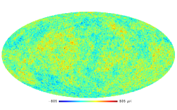
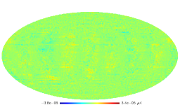
Figure 1: (a) A realization of an unlensed CMB temperature anisotropies map (nside=1024) that we have obtained using NFFT [oversampling factor ($\sigma$)=2, Convolution length $(K)=4$]. (b) Difference of unlensed CMB maps (nside=1024) that we have obtained using NFFT and HEALPix from the same harmonic coefficients.

In Figure 1, we show an (unlensed) realization of the CMB temperature anisotropies obtained using our method, as well as a map of the difference between our method and the HEALPix reference map. Note the difference in the color scales. In order to quantify more precisely the accuracy of our method, we have computed two kinds of error statistics:

$$E_{\infty}^{X} = \frac{max_{j}\left|X_{NFFT}(\theta_{j},\phi_{j})-X_{HEALPix}(\theta_{j},\phi_{j})\right|}{max_{j}\left|X_{HEALPix}(\theta_{j},\phi_{j})\right|}$$

$$E_{2}^{X} = \sqrt{\frac{\sum_{j=1}^{Npix}\left|X_{NFFT}(\theta_{j},\phi_{j})-X_{HEALPix}(\theta_{j},\phi_{j})\right|^{2}}{\sum_{j=1}^{Npix}\left|X_{HEALPix}(\theta_{j},\phi_{j})\right|^{2}}}$$

where $X$ stands for $T$, $Q$, $U$, $d_{\theta}$ and $d_{\phi}$.

$E_{\infty}^{X}$ is the maximum (relative) error for field X, while $E_{2}^{X}$ is the relative root mean square error. Table 1 gives the value of these statistics for unlensed CMB temperature only. Values of these error norms for the displacement field and the unlensed CMB polarization fields are of the same order of magnitude.

Table 1: Variation of typical order of magnitude of error norms with the convolution length $(K)$ for an unlensed CMB map simulated using NFFT. $E_{2}$ and $E_{\infty}$ are the quadratic norm and infinite norm respectively

Oversampling	Convolution	nside	$l_{max}$	Maximum	R. M. S
factor	length			error	error
$\left(\sigma\right)$	$\left(K\right)$			$\left(E_{\infty}\right)$	$\left(E_{2}\right)$
2	4	1024	2048	$\sim 10^{-8}$	$\sim 10^{-8}$
2	6	1024	2048	$\sim 10^{-11}$	$\sim 10^{-12}$
2	8	1024	2048	$\sim 10^{-11}$	$\sim 10^{-13}$

To achieve this accuracy, we have used the Kaiser-Bessel window kunis_potts2008 ; fourmont_2003 as the NFFT interpolating function. Since the full precomputation of the window function at each node in spatial and frequency domains requires lots of memory space, we have used a tensor product form for the multivariate window function, that requires only unidimensional precomputations. This method uses less memory at the price of some extra multiplications kunis_potts2008 ; fourmont_2003 . The accuracy kunis_potts2008 ; fourmont_2003 of our simulation can be improved by increasing both the oversampling factor and the convolution length, at the price of extra memory consumption and CPU time (Table 1).

IV.3 Simulation of lensed maps

We applied our simulation algorithm of lensed CMB maps (both temperature and polarization), as described in Section IV.1, to $1000$ independent realizations with HEALPix resolution $nside=1024$, and a maximum multipole $l_{max}=2048$. In Figure 2, we show one such realization of a lensed CMB temperature field, as well as the difference between the lensed and unlensed fields.

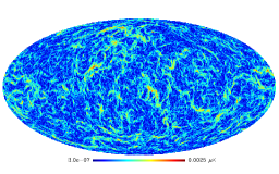
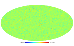
Figure 2: (Top) A realization of lensed CMB map (nside=1024). (Middle) A realization of the amplitude of the deflection field (nside=1024). (Bottom) Difference of lensed and unlensed CMB maps (nside=1024). These maps are obtained using NFFT for the oversampling factor ($\sigma$)=2 and Convolution length $(K)=4$.

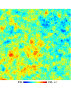
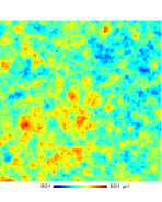
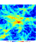
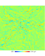
Figure 3: (Top left) A small portion of a simulated unlensed CMB temperature anisotropy map. (Top right). A small portion of the corresponding lensed CMB temperature anisotropy map. (Bottom left) A small portion of the amplitude of the simulated deflection field map. (Bottom right) A small portion of the difference of simulated lensed and unlensed CMB maps. These maps are obtained using NFFT for the oversampling factor ($\sigma$)=2 and Convolution length $(K)=4$.

Since weak lensing of CMB is a tiny effect at small angular scales, we have shown a realization of a small portion of the unlensed CMB temperature anisotropies, lensed CMB temperature anisotropies, amplitude of deflection field and, the difference of lensed and unlensed CMB temperature anisotropies in Figure 3 to better illustrate the lensing effect. Although unlensed and lensed CMB temperature anisotropies are indistinguishable to the naked eye, the correlation between the deflection field and the difference of lensed and unlensed CMB temperature anisotropies is clearly visible.

Table [2] shows the typical CPU time and memory that are required to simulate a single realization of unlensed and lensed CMB temperature and polarization, with different resolutions. Storage of the window function at the grid points both in spatial and frequency domain before computing the Fourier transform consumes a fair amount of memory, which ultimately increases the overall memory requirement for the simulation of lensed CMB mapskunis_potts2008 ; fourmont_2003 .

Table 2: Variation of CPU time and memory requirements with resolution to simulate CMB maps (unlensed and lensed)[oversampling factor ($\sigma$)=2, Convolution length $(K)=4$] using NFFT.

nside	$l_{max}$	CPU	Memory
		time	requirement
256	512	1 min 12 sec	491 MB
512	1024	6 min 8 sec	1.9 GB
1024	2048	32 min	7.6 GB

Table [3] shows the same, but with different convolution lengths. Increase of the convolution length not only increases the computational cost of the interpolation part of NFFT, but also increases the cost of the precomputation of window function and memory requirement as one has to compute and store the window function at a larger number of grid points in the spatial domain before doing NFFTkunis_potts2008 ; fourmont_2003 .

Table 3: Variation of CPU time and memory requirements with the convolution length $(K)$ for simulating a realization CMB map(unlensed and lensed)[nside$=1024$, $l_{max}=2048$] using NFFT.

Oversampling	Convolution	CPU	Memory
factor	length	time	requirement
$\left(\sigma\right)$	$\left(K\right)$
2	4	32 min	7.6 GB
2	6	45 min	8.4 GB
2	8	60 min	9.1 GB

Figure 4 shows on the same plots the theoretical power spectra $C_{l}^{XY}$, where $XY$ stands for $TT,EE,TE,BB$ respectively, for the lensed and unlensed cases, as predicted by CAMB. In the cosmological model we have chosen there are no primordial tensors, hence $C_{l}^{BB}$ is entirely due to lensing.

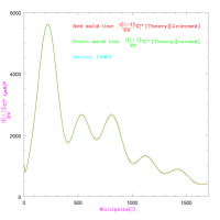
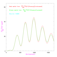
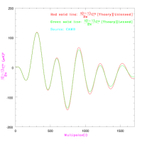
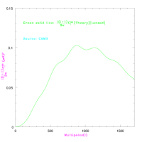
Figure 4: Red solid line is the theoretical angular power spectrum of unlensed CMB, Green solid line is the theoretical angular power spectrum of lensed CMB for temperature

An accurate recovery of this power spectrum from lensed polarization maps is therefore a powerful test of our simulation method. In Figure 5 we show, on top of the lensed theoretical spectra (solid lines), the average empirical power spectra computed from the $1000$ simulations (dots). We can see that the agreement is excellent, which is remarkable for $C_{l}^{BB}$ as explained above. We have ignored the lensed angular power spectrum beyond the multipole $l=1700$ in the comparison of average empirical power spectra and theoretical power spectra because the accurate computation of the average empirical power spectra for the multipoles $l>1700$ requires lensed CMB maps simulated from the power spectra of unlensed CMB and lensing potential beyond the multipole $l=2048$.

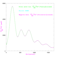
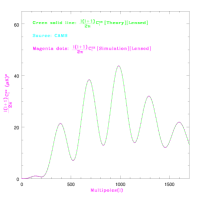
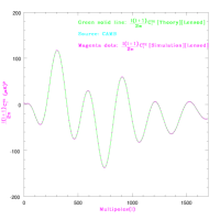
Figure 5: Green solid line is the theoretical angular power spectrum $C_{l,\mathrm{th}}$ of lensed CMB, Magenta dots are the average angular power spectrum $C_{l,\mathrm{simul}}$ recovered from 1000 realizations of lensed CMB maps (nside=$1024$ and $l_{max}=2048$)

To have a more quantitative view of the accuracy of the method, we show in Figure 6 the relative difference between the average empirical power spectra computed on the $1000$ simulations and the theoretical spectra from CAMB, both for the unlensed (red) and lensed (green) cases. On each plot, we also show the theoretical r.m.s. deviation of the averaged empirical spectra, computed neglecting the small lensing-induced non-Gaussianity in the lensed cases. Note that this corresponds to a very small underestimation of the scatter (smith2006 ; rocher2008 ). Taking into account the fact that the averaged power spectra are nearly Gaussian distributed (due to the central limit theorem), we can assess the presence of possible biases in the recovered spectra by computing the reduced $\chi^{2}$ statistics.

$$Z^{2}_{XY}=\frac{N_{rlz}}{(l_{max}-1)}\sum^{l_{max}}_{l=2}\frac{(2l+1)(C^{XY}_{l,\mathrm{simul}}-C^{XY}_{l,\mathrm{th}})^{2}}{\left[(C^{XY}_{l,\mathrm{th}})^{2}+C^{XX}_{l,\mathrm{th}}C^{YY}_{l,\mathrm{th}}\right]}\hskip 10.84006pt$$ (17)

Here $N_{rlz}$ is the number of independent realizations of angular power spectra under consideration.

Table 4: Reduced $\chi^{2}$ statistics for the recovered unlensed angular power spectrum

Angular	Value of
power	$\chi^{2}$	$P(\infty>Z^{2}_{XY}\geq z^{2}_{XY})$
spectrum	statistics
$(C^{XY}_{l,\mathrm{simul}})$	$(z^{2}_{XY})$
$C^{TT}_{l,\mathrm{simul}}$	0.9574	92%
$C^{EE}_{l,\mathrm{simul}}$	0.9879	65%
$C^{TE}_{l,\mathrm{simul}}$	0.9901	62%

Table 5: Reduced $\chi^{2}$ statistics for the recovered lensed angular power spectrum

Angular	Value of
power	$\chi^{2}$	$P(\infty>Z^{2}_{XY}\geq z^{2}_{XY})$
spectrum	statistics
$(C^{XY}_{l,\mathrm{simul}})$	$(z^{2}_{XY})$
$C^{TT}_{l,\mathrm{simul}}$	1.0030	46%
$C^{EE}_{l,\mathrm{simul}}$	0.9928	58%
$C^{BB}_{l,\mathrm{simul}}$	0.9928	58%
$C^{TE}_{l,\mathrm{simul}}$	0.9933	57%

Table 4 & 5 show that the probability of the reduced $\chi^{2}$ statistics $(Z^{2}_{XY})$ having values greater than the estimated values $(z^{2}_{XY})$ are quite large both for unlensed and lensed power spectrum. This strengthens our claim about the unbiasedness in the simulation of unlensed and lensed CMB maps using NFFT.

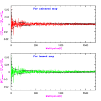
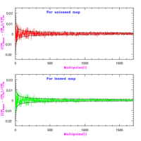
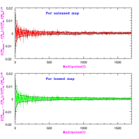
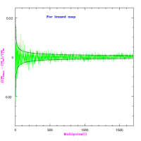
Figure 6: Fractional difference of average angular power spectrua recovered from $1000$ realizations of CMB maps (nside=$1024$ and $l_{max}=2048$) and their corresponding theoretical angular power spectra. Red lines are for unlensed maps and green lines are for lensed maps. Black solid lines show the theoretical cosmic variance.

V Summary

Accurate predictions for the expected CMB anisotropies are required for analyzing future CMB data sets, which ultimately require accurately simulated lensed maps. The most popular pixelization used to analyze full-sky CMB maps is the HEALPix pixelization. In order to simulate lensed CMB anisotropies at HEALPix grid points we have to compute unlensed CMB anisotropies at irregularly spaced grid points over the sphere, determined by the deflection field and remapping equations. Since remapping on a sphere can be recast into remapping on a $2$-d torus, we have used the NFFT library to compute lensed CMB anisotropies at HEALPix grid points and experimented with different settings of the accuracy parameters. We have obtained that for a nside=$1024$ map a $10^{-8}$ accuracy is easily reached when setting the $(\sigma,K)$ parameters to $(2,4)$. With our current implementation of the method, correspond to a $32$ min computation on a classical PC configuration. This can probably be improved by parallelizing the algorithm. Furthermore, the average angular power spectra $C_{l,\,\mathrm{simul}}$ recovered from 1000 realizations of lensed and unlensed CMB maps are also found to be consistent with the corresponding theoretical ones, $C_{l,\,th}$. This validates our simulation of lensed CMB maps.

Such simulations will be a useful tool for the analysis and interpretation of upcoming CMB experiments such as PLANCK and ACT. However, they are not the only possible use of this technique. Indeed, the simulation of the lensing deflection field can be improved by going from the simple Born approximation to ray-tracing through dark matter N-Body simulations. Ray-tracing faces a similar problem as the simulation of the lens effect on CMB maps, i.e. accurately resampling a vector field on the sphere. Current state-of-the-art ray-tracing algorithms, like teyssier2008 could be made more accurate by using the technique described here.

Appendix A Spin $s$ functions on a sphere and 2-d torus

Spin $s$ square-integrable functions ${}_{s}f(\theta,\varphi)$ on a unit sphere are conveniently expanded in spin-weighted spherical harmonics ${}_{s}Y_{lm}(\theta,\varphi)$ of same spin zaldarriaga1997 ; newman1996 ; goldberg1967 .

$${}_{s}f(\theta,\varphi) = \sum_{l=0}^{l_{max}}\sum_{m=-l}^{l}{}_{s}f_{lm}\,\,{}_{s}Y_{lm}(\theta,\varphi)$$ (18)

with the inverse transform,

$${}_{s}f_{lm} = \int_{\Omega}\,d\Omega\,\,{}_{s}f(\theta,\varphi)\,{}_{s}Y_{lm}^{*}(\theta,\varphi)$$ (19)

These harmonics, with $l\in\mathbb{N}$, $m\in\mathbb{Z}$ and max $\left(|m|,|s|\right)\leq l$, form an orthonormal basis for the decomposition of spin $s$ square-integrable functions on the sphere. They are explicitly given in a factorized form in terms of the Wigner rotation matrices $D_{m\,m^{\prime}}^{l}(\varphi,\theta,\rho)$,

$${}_{s}Y_{lm}(\theta,\varphi) = (-1)^{s}\,\sqrt{\frac{2\,l+1}{4\pi}}\,D_{m\,(-s)}^{*\,l}(\varphi,\theta,0)$$ (20)

With our conventions for the Euler angles edmonds1957 ; varshalovich1988 , we have,

$$D_{m\,m^{\prime}}^{l}(\varphi,\theta,\rho) = e^{-i\,m\,\varphi}\,\,d_{m\,m^{\prime}}^{l}(\theta)\,\,e^{-i\,m^{\prime}\,\rho}$$ (21)

These rotation matrices (21) basically characterize the rotation of spin-weighted spherical harmonics. Decomposition shown in equation (21) is exploited by factoring the rotation matrices in two separate rotation matrices as follows wiaux2006 ; mcewen2007 ,

$$D_{m\,m^{\prime}}^{l}(\varphi,\theta,\rho)=\sum_{m^{\prime\prime}}\,D_{m\,m^{\prime\prime}}^{l}\left(\varphi-\frac{\pi}{2},-\frac{\pi}{2},\theta\right)\hskip 21.68121pt$$

$$\hskip 36.135pt\times\,\,D_{m^{\prime\prime}\,m^{\prime}}^{l}\left(0,\frac{\pi}{2},\rho+\frac{\pi}{2}\right)$$ (22)

Expressing the the Wigner rotation matrices (21) in the above manner (22), equation (18) can be rewritten as,

$${}_{s}f(\theta,\varphi)=\sum_{m=-l_{max}}^{l_{max}}\sum_{m^{\prime}=-l_{max}}^{l_{max}}{}_{s}f_{m\,m^{\prime}}\,e^{i(m\,\varphi+m^{\prime}\,\theta)}$$ (23)

where

$${}_{s}f_{m\,m^{\prime}}=\sum_{l=max(|m|,|m^{\prime}|,|s|)}^{l_{max}}\,(-1)^{s}\,\sqrt{\frac{2\,l+1}{4\pi}}\,{}_{s}f_{lm}\hskip 28.90755pt$$

$$\times\,\,\,\,d_{m^{\prime}\,m}^{l}\left(\frac{\pi}{2}\right)\,d_{m^{\prime}\,(-s)}^{l}\left(\frac{\pi}{2}\right)\,\exp\left[-i(m+s)\frac{\pi}{2}\right]\hskip 14.45377pt$$ (24)

The advantage of factoring the rotation matrices in this manner is that now the Euler angles only occur in complex exponentials and we need to evaluate $d_{m\,m^{\prime}}(\theta)$ at $\theta=\frac{\pi}{2}$ only mcewen2007 ; edmonds1957 ; varshalovich1988 ; risbo1996 ; challinor2000 .

Computation of ${}_{s}f(\theta,\varphi)$ using equation (23) may not be the most efficient way, but the presence of exponentials may be exploited such that techniques of fast Fourier transform either on irregular or regular grid may be used for rapid computation of double summations simultaneously. In both cases, the domain of spin $s$ function ${}_{s}f(\theta,\varphi)$ must be extended from the sphere, $(\theta,\varphi)\in[0,\pi]\times[0,2\pi]$ to the 2-dimensional torus, $(\theta,\varphi)\in[0,2\pi]\times[0,2\pi]$ using the symmetry ${}_{s}Y_{lm}(2\pi-\theta,\pi+\varphi)=(-1)^{s}\,{}_{s}Y_{lm}(\theta,\varphi)$ of spin-weighted spherical harmonics so that equation (23) becomes a complex to complex Fourier transform over 2-dimensional torus. The computation of ${}_{s}f_{m\,m^{\prime}}$ for $\left(|m|,|m^{\prime}|\right)\leq l_{max}$, involves performing a 1-dimensional summation over a 2-dimensional grid, hence it is of order ${\cal O}(l_{max}^{3})$.

Appendix B CMB fields on 2-d torus

Factoring the rotation matrices in two separate rotation matrices (21) and extending the domain of CMB, lensing potential and defection fields from sphere to 2-d torus, equations (2,3,7,8) can be rewritten as,

$$T(\theta,\varphi)=\sum_{m=-l_{max}}^{l_{max}}\sum_{m^{\prime}=-l_{max}}^{l_{max}}T_{m\,m^{\prime}}\,\,e^{i(m\,\varphi+m^{\prime}\,\theta)}$$ (25)

$$P(\theta,\varphi)=\sum_{m=-l_{max}}^{l_{max}}\sum_{m^{\prime}=-l_{max}}^{l_{max}}P_{m\,m^{\prime}}\,\,e^{i(m\,\varphi+m^{\prime}\,\theta)}$$ (26)

$$\Phi(\theta,\varphi)=\sum_{m=-l_{max}}^{l_{max}}\sum_{m^{\prime}=-l_{max}}^{l_{max}}\Phi_{m\,m^{\prime}}\,\,e^{i(m\,\varphi+m^{\prime}\,\theta)}$$ (27)

$$\left(d_{\theta}+\,i\,d_{\varphi}\right)\,(\theta,\varphi)\hskip 130.08621pt$$

$$=\sum_{m=-l_{max}}^{l_{max}}\sum_{m^{\prime}=-l_{max}}^{l_{max}}G_{m\,m^{\prime}}\,\,e^{i(m\,\varphi+m^{\prime}\,\theta)}$$ (28)

and the corresponding Fourier modes are given by,

$$T_{m\,m^{\prime}}=\sum_{l=max(|m|,|m^{\prime}|)}^{l_{max}}\sqrt{\frac{2\,l+1}{4\pi}}\,\,T_{lm}\hskip 90.3375pt$$

$$\times\,\,d_{m^{\prime}\,m}^{l}\left(\frac{\pi}{2}\right)\,d_{m^{\prime}\,0}^{l}\left(\frac{\pi}{2}\right)\,\exp\left[-im\frac{\pi}{2}\right]\hskip 18.06749pt$$ (29)

$$P_{m\,m^{\prime}}=\sum_{l=max(|m|,|m^{\prime}|,2)}^{l_{max}}\,\sqrt{\frac{2\,l+1}{4\pi}}\,(E_{lm}+i\,B_{lm})\hskip 36.135pt$$

$$\times\,\,d_{m^{\prime}\,m}^{l}\left(\frac{\pi}{2}\right)\,d_{m^{\prime}\,(-2)}^{l}\left(\frac{\pi}{2}\right)\,\exp\left[-im\frac{\pi}{2}\right]\hskip 18.06749pt$$ (30)

$$\Phi_{m\,m^{\prime}}=\sum_{l=max(|m|,|m^{\prime}|)}^{l_{max}}\sqrt{\frac{2\,l+1}{4\pi}}\,\Phi_{lm}\hskip 90.3375pt$$

$$\times\,\,d_{m^{\prime}\,m}^{l}\left(\frac{\pi}{2}\right)\,d_{m^{\prime}\,0}^{l}\left(\frac{\pi}{2}\right)\,\exp\left[-im\frac{\pi}{2}\right]\hskip 18.06749pt$$ (31)

$$G_{m\,m^{\prime}}=\sum_{l=max(|m|,|m^{\prime}|,1)}^{l_{max}}(-i)\sqrt{\frac{l\,(l+1)\,(2\,l+1)}{8\pi}}\,\Phi_{lm}\hskip 25.29494pt$$

$$\times\,\,d_{m^{\prime}\,m}^{l}\left(\frac{\pi}{2}\right)\,d_{m^{\prime}\,(-1)}^{l}\left(\frac{\pi}{2}\right)\,\exp\left[-im\frac{\pi}{2}\right]\hskip 18.06749pt$$ (32)

- (1) A. Blanchard and J. Schneider, Astronomy and Astrophysics, vol. 184, no. 1-2, 1-6 (1987).
- (2) Uros Seljak, Astrophys.J. 463, 1 (1996).
- (3) Matias Zaldarriaga and Uros Seljak, Phys.Rev. D58 023003 (1998).
- (4) W.Hu, M.Tegmark, Astrophys. J. Lett. 514, 65 (1999).
- (5) Wayne Hu, Astrophys.J. 522 (1999) L21-L24.
- (6) Matias Zaldarriaga, Uros Seljak, Phys.Rev. D59, 123507 (1999).
- (7) Jacek Guzik, Uros Seljak and Matias Zaldarriaga, Phys.Rev. D62, 043517 (2000).
- (8) L. Van Waerbeke, F. Bernardeau, K. Benabed, Astrophysical Journal 540, 14-19 (2000).
- (9) K. Benabed, F. Bernardeau, L. van Waerbeke, Phys.Rev. D63 043501 (2001).
- (10) Wayne Hu, Phys.Rev. D62, 043007 (2000).
- (11) Wayne Hu, Takemi Okamoto, Astrophys.J. 574, 566-574 (2002).
- (12) Michael Kesden, Asantha Cooray and Marc Kamionkowski, Phys.Rev. D 66 083007 (2002).
- (13) Christopher M. Hirata and Uros Seljak, Phys.Rev. D67 043001 (2003).
- (14) Christopher M. Hirata and Uros Seljak, Phys.Rev. D68 083002 (2003).
- (15) Michael Kesden, Asantha Cooray and Marc Kamionkowski, Phys.Rev. D 67, 123507 (2003).
- (16) Christopher M. Hirata, Nikhil Padmanabhan, Uros Seljak, David Schlegel, and Jonathan Brinkmann, Phys. Rev. D 70, 103501 (2004).
- (17) Sudeep Das and Paul Bode, Astrophys. J. 682, 1 (2008).
- (18) Antony Lewis, Phys. Rev. D 71, 083008 (2005).
- (19) Anthony Challinor and Antony Lewis, Phys. Rev. D 71, 103010 (2005).
- (20) Antony Lewis and Anthony Challinor, Physics Reports, Volume 429, Issue 1, June 2006, Pages 1-65.
- (21) Kendrick M. Smith, Oliver Zahn and Olivier Dore, Phys. Rev. D 76, 043510 (2007).
- (22) Laurence Perotto, Julien Lesgourgues, Steen Hannestad, Huitzu Tu, Yvonne Y.Y. Wong, CAP 0610, 013 (2006).
- (23) Julien Lesgourgues, Laurence Perotto, Sergio Pastor, Michel Piat, Phys.Rev. D73 045021 (2006).
- (24) A. H. Guth, Phys. Rev. D 23, 347 (1981).
- (25) A. D. Linde, Phys. Lett. B 108, 389 (1982).
- (26) A. Albrecht and P. J. Steinhardt, Phys. Rev. Lett. 48, 1220 (1982).
- (27) Asantha Cooray, Wayne Hu, Jordi Miralda-Escude, Astrophys.J. 535 (2000) L9-L12.
- (28) Asantha Cooray and Wayne Hu, Astrophys.J. 548, 7 (2001).
- (29) A.R.Cooray and W.Hu, Astrophys. J. 554, 56 (2001).
- (30) Asantha Cooray and Wayne Hu, Astrophys.J. 574, 19 (2002).
- (31) Takemi Okamoto and Wayne Hu, Phys.Rev. D 67, 083002 (2003).
- (32) W.Hu, T.Okamoto, Phys. Rev. D 69 043004 (2004).
- (33) http://cosmologist.info/lenspix
- (34) http://www-user.tu-chemnitz.de/potts/nfft
- (35) S. Kunis and D. Potts, Sampling Theory in Signal and Image Processing, 7, 77-100 (2008).
- (36) K. Fourmont, J. Fourier Anal. Appl., 9 ,431-450, (2003).
- (37) http://www.fftw.org
- (38) Matias Zaldarriaga and Uros Seljak, Phys. Rev. D 55 , 1830 (1997).
- (39) E. Newman and R. Penrose, J. Math Phys 7, 863 (1966).
- (40) J. N. Goldberg et al., J. Math Phys. 8, 2155 (1967).
- (41) K.S. Thorne, Rev. Mod. Phys. 52, 299 (1980).
- (42) A. R. Edmonds, Princeton University Press (1957).
- (43) D. A. Varshalovich, A. N. Moskalev, V. K. Khersonskii, Singapore: World Scientific, (1988).
- (44) Y. Wiaux, L. Jacques, P. Vielva and P. Vandergheynst,Astrophys.J. 652, 820, (2006)
- (45) J. D. McEwen, M. P. Hobson, D. J. Mortlock, A. N. Lasenby, IEEE Trans.Signal Process. 55, 520-529,(2007).
- (46) T. Risbo, J. Geodesy, Berlin 70, 383 (1996).
- (47) Anthony Challinor, Pablo Fosalba, Daniel Mortlock, Mark Ashdown, Benjamin Wandelt, and Krzysztof Gorski, Phys. Rev. D 62, 123002 (2000).
- (48) Benjamin D. Wandelt and Krzysztof M. Gorski, Phys. Rev. D 63, 123002 (2001).
- (49) http://camb.info
- (50) K.M. Górski, Eric Hivon, A.J. Banday, B.D. Wandelt, F.K. Hansen, M. Reinecke, M. Bartelmann, ApJ, 622, 759 (2005)
- (51) J. Rocher, K. Benabed and F.R. Bouchet, JCAP 5,13 (2007)
- (52) K.M. Smith, W. Hu and M. Kaplinghat, Phys. Rev. D, 74,123002 (2006)
- (53) R. Teyssier et al., astro-ph/0807.3651, (2008)