Tests of AMiBA Data Integrity

Abstract

We describe methods used to validate data from the Y.T. Lee Array for Microwave Background Anisotropy (AMiBA), an interferometric array designed to measure the Sunyaev-Zel’dovich effect and the anisotropy of the Cosmic Microwave Background (CMB). We perform several statistical tests on data from pointed galaxy cluster observations taken in 2007 and noise data from long-term blank sky observations and measurements with the feeds covered by the absorbers. We apply power spectrum analysis, cross power spectrum analysis among different outputs with different time lags in our analog correlator, and sample variance law tests to noise data. We find that (1) there is no time variation of electronic offsets on the time scale of our two-patch observations ($\sim 10$ minutes); (2) noise is correlated by less than 10% between different lags; and (3) the variance of noise scales with the inverse of time. To test the Gaussianity of the data, we apply Kolmogorov-Smirnov (K-S) tests to cluster data, and find that a 5% significance level efficiently detects data sets with known hardware problems without rejecting an excess of acceptable data. We also calculate third- and fourth-order moments and cumulants for the noise residual visibilities and find that about 95% of our data are within the 99% confidence regions of Gaussianity.

1 Introduction

Measurements of the Cosmic Microwave Background (CMB) on arcminute scales reveal the large-scale structure of the Universe and probe the gas properties of galaxy clusters through the Sunyaev-Zel’dovich effect (SZE). Since the CMB signals on such small angular scales are quite weak, long integrations are necessary to achieve detections. Consequently the noise properties and system stability become crucial problems for CMB projects. Instability and non-Gaussianity of the noise often arise from hardware issues or unexpected noise sources in the system, which may cause systematic errors in the measurements and lead to incorrect scientific interpretation. Many CMB projects therefore expend significant effort on testing the noise properties of their data (e.g., de Bernardis et al., 2000; Padin et al., 2001; Halverson el al., 2002; Grainge et al., 2003; Hinshaw et al., 2003; Smith et al., 2004; Kuo et al., 2004; Savage et al., 2004; Rubino-Martin et al., 2006; Watson et al., 2003; Wu et al., 2001; Jarosik et al., 2007; Wu et al., 2007; Muchovej et al., 2008).

This paper is one of a series of papers reporting the first results from the Y.T. Lee Array for Microwave Background Anisotropy (AMiBA) (Ho et al., 2008). AMiBA is an interferometric array designed to measure the anisotropy of the Cosmic Microwave Background (CMB) and the SZE which has the dual-channel 86-102 GHz operating frequency (Chen et al., 2008). The site is located on Mauna Loa, Hawaii at 3396m altitude. Seven 60-cm antennas are mounted on the 6-m configurable platform in the compact configuration in the current setup which is capable of an expansion to 19 elements. Operation with 13 elements is planned to start in early 2009. The first run of the science operations was carried out in 2007 and a total of six galaxy clusters are detected through the SZE. The analysis results of these clusters are reported in a series of papers (Wu et al., 2008; Umetsu et al., 2008; Koch et al., 2008a; Huang et al., 2008, AMiBA cluster papers hereafter).

The aim of this paper is to test the integrity of our data by performing statistical tests of the noise in our system, and thus to provide the basis on which the results of the AMiBA cluster papers are founded. Some other possible sources of systematic error are discussed in other papers. Detailed descriptions of the system performance and calibration are discussed in Lin et al. (2008). Pointing accuracy and antenna misalignment are discussed in Koch et al. (2008b). The level of contamination of SZE measurements from primary CMB fluctuations and radio sources or other foregrounds is discussed in Liu et al. (2008). The overall data flagging is described in Wu et al. (2008).

This paper is organized as follows. In section 2, we discuss the statistical properties of the noise data. In section 3, the Gaussianity tests of our data from cluster observations are described. Section 4 is devoted to the Conclusions.

2 Statistical tests of the noise in our system

In this section we describe the noise properties of our system from the long-term noise data. The data were taken in two different ways. First, we took data with the feeds covered by absorbers that block all signals, for periods of one day to five days. Second, we made blank sky observations lasting about one hour to eight hours at night (after sunset to before sunrise), where the telescope was parked pointing to the zenith (declination +19.5 degrees) — we confirmed that no strong source passes through the field of view. Multiple such datasets have been taken and similar characteristics were found in all cases. Representative results are shown below. Furthermore, we find no significant differences in the results of the statistical analyses described below between data taken in these two different ways.

AMiBA is an interferometer with 4-lag analog correlators which output real-number correlation signals. We denote the time-ordered outputs from our correlators at time $t$ as $\mbox{\boldmath$c$}(t)=\{c_{i}(t):i=1,4\}$ in units of counts from the A/D converter with the time interval of 0.452 seconds where $i=1,...,4$ is the lag number (see Li et al., 2004). We define the power spectrum as

$$P_{ij}(\nu)={\hat{c}_{i}(\nu)\hat{c}_{j}^{*}(\nu)\over T},$$ (1)

where $\nu$ is the frequency, $\hat{c}$ is the Fourier transform of $c(t)$, and ^∗ denotes complex conjugation. The power spectrum is normalized by $T$, the total length of data.

2.1 Long time scale variation of the electronic offset

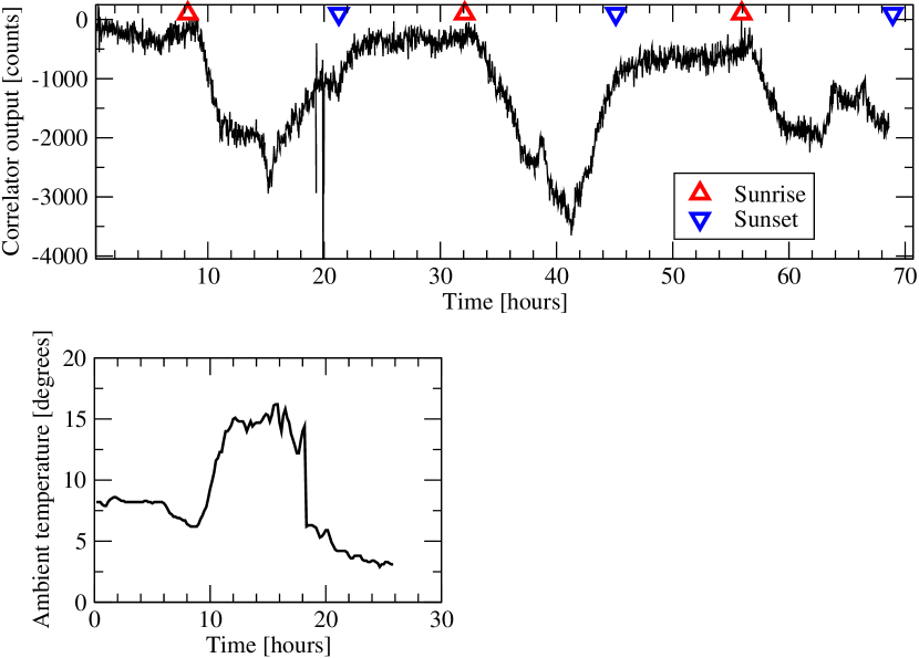
Figure 1: The variation of the correlator outputs over about three days of data. Average counts over two-minute periods are shown as a function of time. A strong diurnal pattern is seen, with rapid changes at the times of sunrise and sunset (marked by the red triange-up and blue triangle-down, respectively). The lower panel shows ambient temperature variations for about one day monitored over the same period.

Figure 1 shows the time variation of the correlator outputs as a function of time over three days of absorber data. The correlator outputs are averaged over two minutes to show the long-period variations more clearly. Although there is no astronomical signal in this data, the correlator outputs show time-variable and non-zero electronic offsets. Our data analysis procedure subtracts these offsets by adopting a two-patch procedure, where the telescope first tracks a science target for some time, and then moves to a blank-sky patch that trails the science target and follows the same set of mount positions (Wu et al., 2008). This ensures that electronic offsets and ground pick up signals that depend on mount position are accurately subtracted, provided that the time-scale of variation of these contaminating signals is sufficiently slow (Wu et al., 2008).

Figure 1 shows a strong diurnal variation in the correlator outputs which parallels ambient temperature variations. The most rapid changes in correlator signal occur at the sunrise and sunset, when the temperature changes quickly. At night, when the temperature variation is slow, the outputs are relatively stable. We avoid making observations near sunrise and sunset to exclude systematic errors from such rapid system changes. The results from the observations in 2007 reported in the AMiBA cluter papers are based on data taken only at night. We also carried out long-term tracking of the bright planets to examine the overall stability of the system including the effects from the atmosphere. From this test we concluded that gain and phase calibrations every two to three hours are necessary (Lin et al., 2008).

It is important to quantify the time scales of correlator variations to define the switching time for our two-patch method. We discuss this issue in the next section, through Fourier analysis.

2.2 Noise Power Spectrum

If the time scale of the variation of the offsets is shorter than the switching interval in our two-patch procedure, then our data will be strongly contaminated by an error signal. To examine the time variation of the offsets, we perform a power spectrum analysis (the case of $i=j$ in equation (1)) of the noise data.

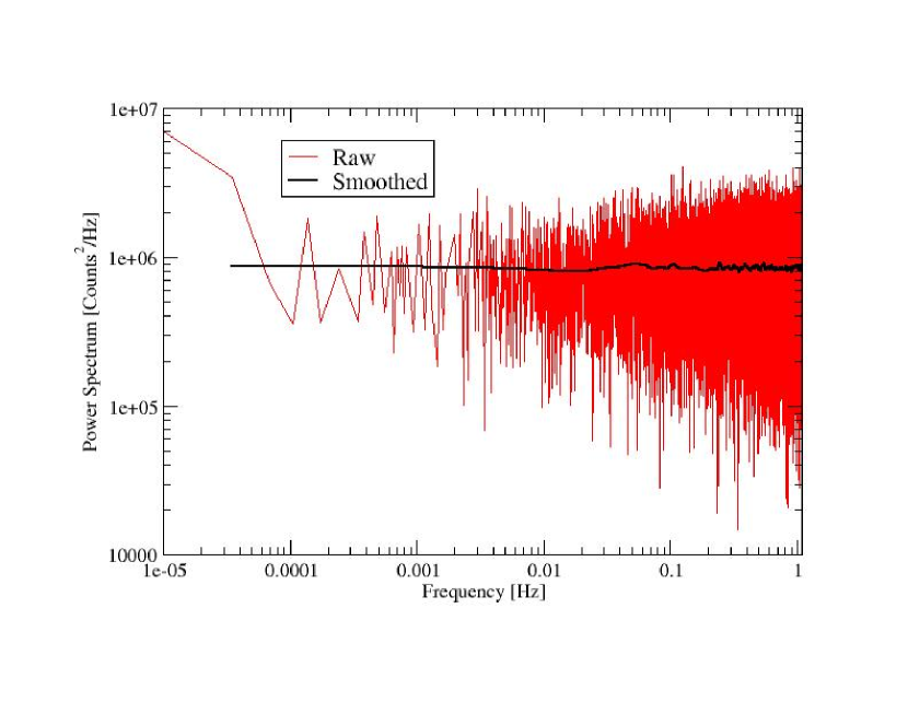
Figure 2: The noise power spectrum from an eight-hour absorber data. The red and black curves represent the raw and smoothed power spectra, respectively. The spectra are indicative of white noise over the frequency range $0.0001$ to $1$ Hz. To reduce the sample variance, three sets of 8-hour spectra are averaged.

Figure 2 shows the measured noise power spectrum for eight hours of data taken at night. The red curve shows the raw power spectrum, while the black curve shows the power spectrum smoothed by a Gaussian kernel with $\sigma=0.005$ Hz to show the characteristics of the data more clearly. To reduce the sample variance, three sets of 8-hour spectra are averaged. The spectrum has white-noise form over frequencies between $10^{-4}$ and 1 Hz, with an increase in power at lower frequency because of slow variations of the offsets. Based on these results, we expect that two-patch data taken with an interval of less than 600 sec (typical for our observing procedure) will not be contaminated by variations of the electronic offsets.

2.3 Noise Correlation among Lags

Each correlator output dataset consists of a time-ordered series of four numbers corresponding to the correlated signals from each of the four time lags. These four output numbers are transformed to the real and imaginary parts of two complex visibilities, representing the upper and lower frequency channels, in the first stages of data processing (Wu et al., 2008). Since this process is a linear transformation, noise correlation between different lag outputs leads to non-zero non-diagonal components of the noise correlation matrix, and this feeds through to the covariance matrix of the visibilities and error estimates. To examine how the noise from different lags correlates, we compute the cross power spectrum between lags.

The strength of the correlation is quantified by the correlation coefficient defined by

$$r={P_{ij}(\nu)\over\sqrt{P_{ii}(\nu)P_{jj}(\nu)}},$$ (2)

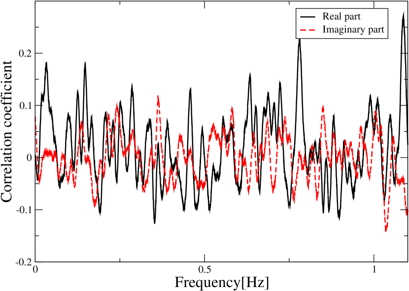
Figure 3: The correlation coefficient among lags(the adjacent lag, $i=1,j=2$) fron the blank sky data. The black-solid and red-dashed curves represent real and imaginary parts, respectively. The real part fluctuates around a positive value $\sim 0.03$. There is no significant frequency dependence of $r$ and the level of correlation between lags is generally less than 10%.

where $r$ is a complex number. The real part of $r\rightarrow 1$ if lags $i$ and $j$ show perfect correlation. If there is no correlation, then $r\rightarrow 0$. Figure 3 shows the real and imaginary parts of the correlation coefficient between the adjacent lags, $i=1,j=2$. We do not find any different characteristics of the cross correlation between distant lags (e.g. $i=1,j=3$ and $i=1,j=4$). To see the cross-correlation properties clearly, we apply smoothing by a Gaussian kernel with $\sigma=0.05$ Hz.

We see that the imaginary part of $r$ fluctuates around zero while the real part fluctuates around a positive value $\sim 0.03$, which suggests the existence of correlated noise between lags. However, we find no significant frequency dependence of $r$, and it is clear from Fig. 3 that the level of correlation between lags is generally less than 10%. We note that there are some exceptions to this limit, where stronger correlation is found (sometimes more than 20%), but this is a characteristic of correlators with temporary hardware problems where the data would not be used in later analysis.

2.4 Sample Variance Law test

In our science observations we rely on the reduction of the noise level through long integrations. The rate at which the noise reduces in time is an important indicator of the effectiveness of the AMiBA system, and we would hope that noise fluctuations decrease in time following the sample variance law. We test this by calculating whether the variance of the noise power spectrum decreases as the length of the data chunk used for the spectrum increases. We apply the test by
(i) dividing the raw datasets of the noise into short chunks with different lengths
(ii) calculating the power spectrum for each chunk
(iii) calculating the variance of the chunk power spectra over the entire dataset
(iv) comparing the variances from different chunk lengths.
The variance is defined by

$${\rm variance}={1\over N}\sum_{i}^{N}P_{\rm chunk}^{2}(i,\nu)-\left[{1\over N}\sum_{i}^{N}P_{\rm chunk}(i,\nu)\right]^{2}\quad,$$ (3)

where $P_{\rm chunk}(i,\nu)$ is the power spectrum of the $i$-th chunk and $N$ is the number of chunks.

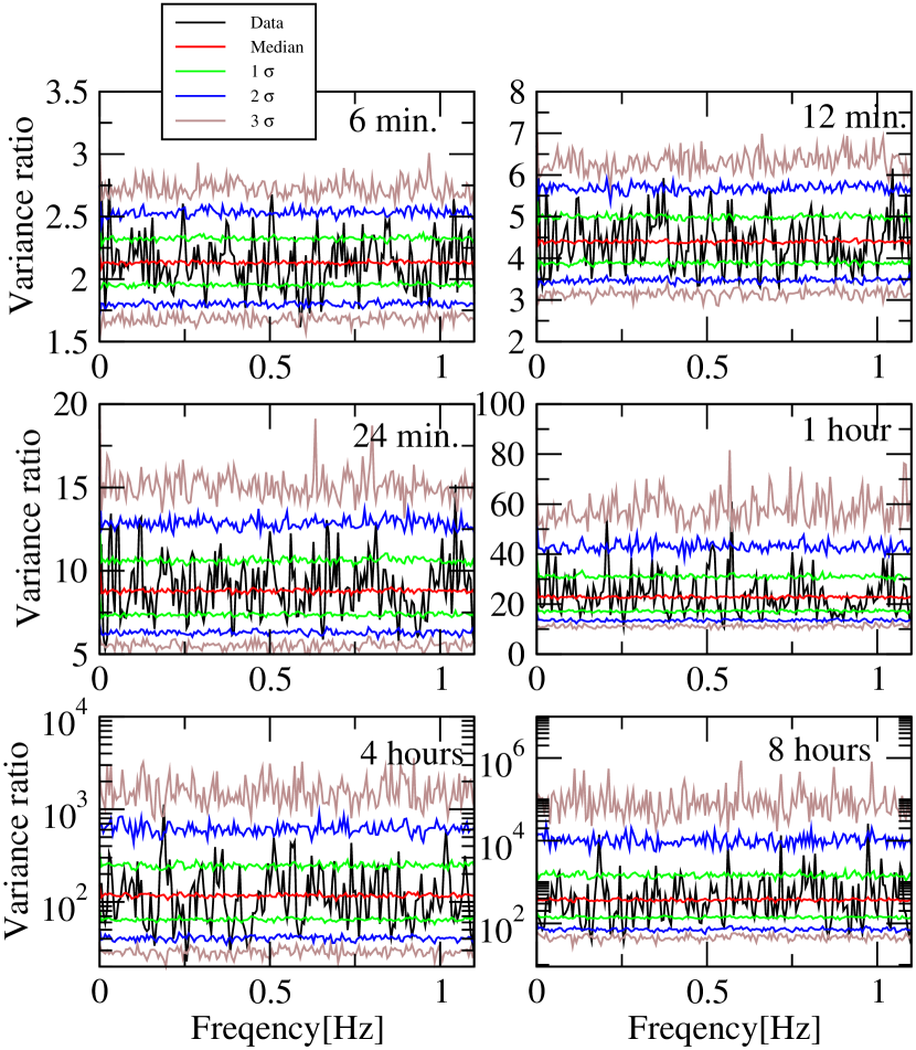
Figure 4: Variance ratios of 3-minute chunk power spectrum to the 6-minute to 8-hour chunk spectra from the absorber data. The black curves represent the variance ratios, and the green, blue and brown lines represent the 1, 2 and 3$\sigma$ confidence levels derived from 500 Monte-Carlo simulations assuming Gaussian random noise with the same noise power as our data. The red lines represent the medians from the simulations.

Figure 4 shows the variance ratio, which is the variance of the power spectra for 3-minute chunks divided by the variances for 6 minutes to 8 hours-chunks. In this analysis 24 hours data (made up from three sets of eight-hour datasets taken at night) is used. The black curves represent the measured variance ratio spectra. It is seen that the variance ratios fluctuate around the median from 500 Monte Carlo simulations (red lines) as expected if the chunk power follows the sample variance law. The green, blue and brown lines represent the 1, 2 and 3$\sigma$ confidence levels derived from the simulations. In the simulations we assume Gaussian random noise with a flat power spectrum with the same level of power as the data. The results are consistent with the Monte Carlo simulations within 3-$\sigma$ confidence limits, except for a few data points that we can trace to spurious correlator outputs that have negligible effect on our analyses or science results. The integration times of the observed galaxy clusters are five to eleven hours (Wu et al., 2008). The reduction of noise with integration demonstrated here assures us of the reliability of our cluster results.

For our observations of galaxy clusters, the contribution from the brightest contaminants in the night sky, the Moon and the planets, is crucial. We also investigate it here using the measured primary beam pattern and the simulated correlator data (Wu et al., 2008). In the 2-patch observing strategy, when the offset direction of the Moon is perpendicular to the baseline by 10 and 40 degrees and the two-patch link direction is also perpendicular to the baseline, the attenuation in Moon signal is by an order of $10^{-5}$ and $10^{-6}$ respectively. Such attenuation is mainly from the attenuation of the primary beam. When the offset direction is along the baseline direction and the two-patch link direction is also aligned with the baseline, attenuation of at least one extra order appears due to the frequency-band smearing effect of the correlators.

qWe have carefully checked the angular separation between these contaminants and our cluster targets, and found that it was at least 10 degrees, mostly beyond 50 degrees. We finally verified that after the flagging and the integration over the hours that may be from various days, the contribution from either the Moon or the planets is at least two orders below our cluster signals.

3 Gaussianity of the data

If the data are non-Gaussian in their statistics, then the data are likely to contain systematic errors, and the errors are likely to be badly estimated. In this section we apply several statistical tests to cluster SZE data to verify the Gaussianity of our system noise in the lag and visibility data.

3.1 Gaussianity tests in correlator outputs

Since our science observations are based on the two-patch method described above, the data from each patch should be a constant signal plus noise. If the noise follows a Gaussian distribution, all our data also should follow a Gaussian distribution centered on the astronomical signal. To test the Gaussianity of our data, we adopt a Kolmogorov-Smirnov (K-S) test which is commonly used to judge whether two distributions are different at a certain significance level. In the K-S test, we measure the maximum value of the absolute difference between two cumulative distribution functions,

$$D=\max_{-\infty<x<\infty}\left|S_{\rm data}(x)-S(x)\right|,$$ (4)

where $S_{\rm data}(x)$ is the cumulative distribution of the correlator outputs. The cumulative distribution $S(x)$ which is to be compared with the data is derived from the Gaussian distribution centered at the mean signal and with a standard deviation estimated from the rms deduced from data during observations of a single patch. The maximum distance $D$ is a measure of how much different the two distributions are. The low significance level is induced by the large value of $D$ and means that the difference between two distributions is significant.

We apply this test to the data and find that our K-S tests at a 5% significance level can successfully detect correlators that are known to provide bad data because of hardware problems. The tests with lower significance levels reduce a success rate in detection of the problems. Apart from these known bad correlators, more than 90% of the data pass the K-S tests at the 5% significance level. Figure 5 shows example correlator outputs for one patch of observation. The upper left panel shows an output lag dataset that passes the K-S test. The other panels are examples where the outputs fail the K-S test at the 5% level. While the example shown in the top right panel is obvious, the examples in the lower two panels are less clear, although all three datasets were known to have hardware problems at the time that these data were taken. (The problem was temporary and quickly fixed). This suggests that K-S tests at a 5% level provide a useful diagnostic for hardware problems. In our analysis procedure we remove all datasets identified by such a K-S test.

3.2 Gaussianity tests in visibilities

We also apply Gaussianity tests to the visibilities. Since the visibilities from cluster observations include signal and noise, we must subtract the astronomical signals to investigate the residual noises. In our analysis we subtract the mean of the visibilities, and investigate the third- and fourth-order moments and cumulants from the residuals. We analyze the visibility data for the real and imaginary parts of the lower and upper frequency bands separately. We find that about 95% of our data from the six clusters described by Wu et al. (2008) are consistent with Gaussianity within 99% confidence limits as derived from 500 Monte-Carlo simulations (more realizations do not change the results). Although this result implies that there is a small level of non-Gaussian noise present, this has no important effect on the statistics.

4 Conclusions

We have performed several statistical tests to noise data from blank sky observations and the measurements with the feeds covered by the absorbers, and observations of galaxy clusters to demonstrate the integrity of AMiBA data. The noise data has been analyzed through their power spectra, lag-lag cross-correlations, and sample variance law.

From the power spectrum analysis we have found that there are no significant time variations of the electronic offsets on time scales shorter that the time scale of our two-patch observing procedure. This demonstrates that our science data is free of systematic errors introduced by fast system drifts.

Cross power spectrum analysis has been applied to examine the noise correlation between different lags. This revealed a weak correlation, at the level of less than 10%.

To examine whether the noise decreases over long integrations, we have applied the sample variance law test to long-duration blank-sky data. The data were divided into several chunks with different lengths in time and the variances of the power spectra were calculated and compared. We showed that the fluctuations of chunk power follow the sample variance law to the time scales of the integration times of galaxy clusters to within the errors estimated from Monte Carlo simulations assuming that the data are scattered only by Gaussian random noise with the same power.

To test the Gaussianity of our data we applied statistical tests to the lag and visibility data. We found that K-S tests with 5% significance can clearly detect lag and visibility data known to be bad because of hardware issues. This led us to adopt a K-S test at this level to check all AMiBA data for hardware problems. Except for such known bad lag data, more than 90% of the data passes such K-S tests.

We have also performed Gaussianity tests on the visibility data. We calculated third- and fourth-order moments and cumulants of the residual noise visibilities, and found that about 95 % of our data are within the 99% confidence region of Gaussianity derived from the Monte Carlo simulations. The apparent residual level of non-Gaussianity (4%) is not expected to affect the analysis of AMiBA data.

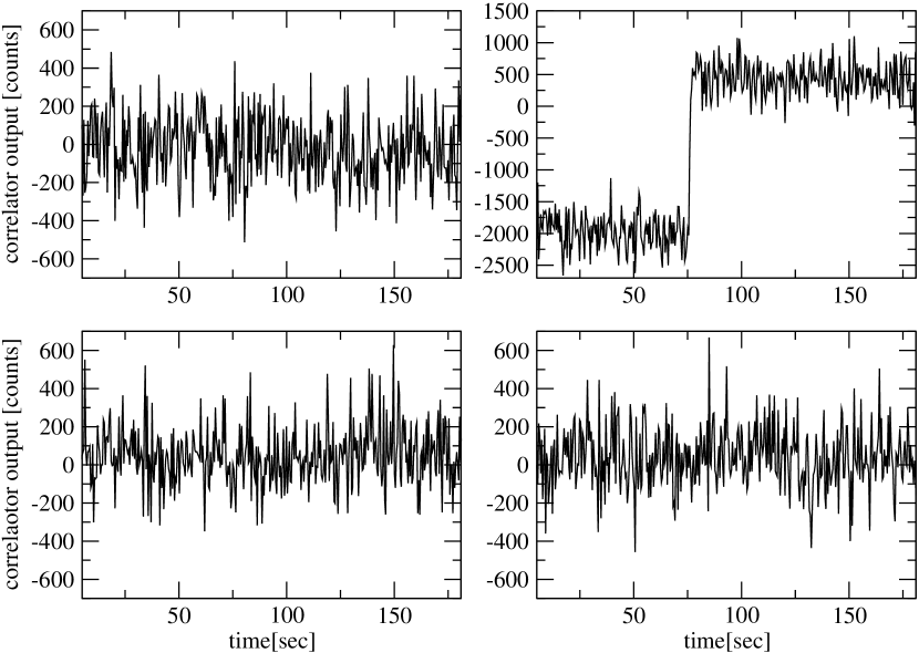
Figure 5: Examples of correlator outputs as a function of time for one patch of a two-patch cluster observation. The top left panel an output that passes the K-S test. The other panels are examples of outputs that fail the K-S test for obvious (top right) or more subtle (bottom left and bottom right) reasons.

References

- de Bernardis et al. (2000) de Bernardis, P. et al. 2000, Nature, 404, 955
- Chen et al. (2008) Chen, M.-T. et al. 2008, in preparation
- Halverson el al. (2002) Halverson, N. W., Leitch, E. M., Pryke, C., Kovak, J., Carlstrom, J. E., Holzapfel, W. L., & Dragovan, M., 2002, ApJ, 568, 38
- Ho et al. (2008) Ho, P.T.P. et al. 2008, ApJ, submitted (arXiv:0810.1871)
- Hinshaw et al. (2003) Hinshaw, G. et al. 2003, ApJS, 148, 63
- Huang et al. (2008) Huang, C.-W.L. et al. 2008, in preparation
- Jarosik et al. (2007) Jarosik, N. et al. 2007, ApJS, 170, 263
- Koch et al. (2008a) Koch, P.M. et al. 2008a, in preparation
- Koch et al. (2008b) Koch, P.M. et al. 2008b, in preparation
- Kuo et al. (2004) Kuo, C.L. et al. 2008, ApJ, 600, 32
- Li et al. (2004) Li, C.-T. et al. 2004, SPIE, 5498, 455
- Lin et al. (2008) Lin, K.-Y. et al. 2008, in preparation
- Liu et al. (2008) Liu, G.-C. ,et al. 2008, in preparation
- Muchovej et al. (2008) Muchovej, S. et al., 2007, ApJ, 663, 708
- Padin et al. (2001) Padin, S. et al. 2001, ApJ, 549, L1
- Grainge et al. (2003) Grainge, K. et al. 2003, MNRAS, 341, L23
- Smith et al. (2004) Smith, S., et al. 2004, MNRAS, 352, 887
- Savage et al. (2004) Savage, R. et al. 2004, MNRAS, 249, 973
- Rubino-Martin et al. (2006) Rubino-Martin, J. A. et al. 2006, MNRAS, 369, 909
- Umetsu et al. (2008) Umetsu, K. et al. 2008, ApJ, submitted (arXiv:0810.0969)
- Watson et al. (2003) Watson, R. A. et al. 2003, MNRAS, 341, 1057
- Wu et al. (2001) Wu, J. H. P. et al. 2001, Phys. Rev. Lett., 87, 251303
- Wu et al. (2007) Wu, J. H. P. et al. 2007, ApJ, 665, 55
- Wu et al. (2008) Wu, J. H. P. et al. 2008, ApJ, submitted (arXiv:0810.1015)