Explicit illustration of non-abelian fusion rules in a small spin lattice

Yue Yu Institute of Theoretical Physics, Chinese Academy of Sciences, P.O. Box 2735, Beijing 100190, China    Tieyan Si Institute of Theoretical Physics, Chinese Academy of Sciences, P.O. Box 2735, Beijing 100190, China
Abstract

We exactly solve a four-site spin model with site-dependent Kitaev’s coupling in a tetrahedron by means of an analytical diagonalization. The non-abelian fusion rules of eigen vortex excitations in this small lattice model are explicitly illustrated in real space by using Pauli matrices. Comparing with solutions of Kitaev models on large lattices, our solution gives an intuitional picture using real space spin configurations to directly express zero modes of Majorana fermions, non-abelian vortices and non-abelian fusion rules. We generalize the single tetrahedron model to a chain model of tetrahedrons on a torus and find the non-abelian vortices become well-defined non-abelian anyons. We believe these manifest results are very helpful to demonstrate the nonabelian anyon in laboratory.

pacs:
75.10.Jm,03.67.Pp,71.10.Pm

The spin lattice models of Kitaev-type have attracted many research interests because of the abelian and nonabelian anyons in these exactly soluble two-dimensional models kitaev ; kitaev1 , which are of the potential application in the topological quantum memory and fault-tolerant topological quantum computation rev .

The abelian anyons can be explicitly shown in Kitaev toric code model kitaev or Levin-Wen model lw . Fusion rules and braiding matrix can be easily illustrated in real space. This has simulated many attempts to design and process experiments to demonstrate these abelian anyons in laboratory exp .

In solving Kitaev honeycomb model kitaev and its ramifications yuwang ; yao1 ; wuc , a key technique is the usage of the Majorana fermion representation of the spin-1/2 operators. The systems then are transferred into bilinear fermion systems and the ground state sector can be diagonalized in the momentum space. The shortcoming to use the momentum space is that the ground state and the elementary excitations are hard to be expressed by the original spin operators, i.e., Pauli matrices. On the other hand, the sectors with vortex excitations can only be treated numerically. Then the nonabelian fusion rules and statistics may not be directly shown in Pauli matrices’ language. Lahtinen et al have derived the nonabelian fusions through the spectrum analysis la . However, they are still not directly related to Pauli matrices. A real space form of the ground state of the Kitaev honeycomb model in the insulating phase with abelian anyon was studied cn . We tried to present the non-abelian fusion rules for high energy excitations in this Kitaev model yusi . There was an attempt to use toric code abelian anyons to superpose the Ising non-abelian anyons without involving a Hamiltonianwang .

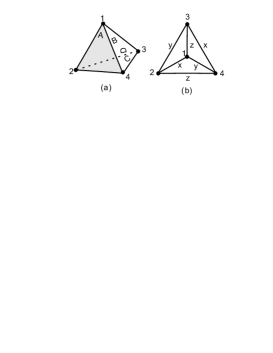
In this paper, we solve a spin model with Kitaev’s coupling in a small lattice, i.e., a tetrahedron (Fig.1). We perform Majorana fermions and their zero modes, non-abelian vortices and their fusion rules in real space by means of Pauli matrices. Because the system is finite and everything can be deduced in an elemental way, it will be very helpful to intuitionally understand these concepts which were used to be expressed in those deep mathematical language. Since the spin configurations of these excitations and the fusion rules are explicitly shown, the experimental techniques with cold atoms, finite photon graph states and nuclear magnetic resonance systems exp are possible to be applied to demonstrate these quantum states and then to design quantum bits and gates for a topological quantum computer.

The single tetrahedron model is too small for non-abelian anyons to be well-defined. We generalize it to be a chain model of tetrahedrons on a torus. This chain model is also exactly solvable and the non-abelian anyons can be well-defined. They are still of a simple form like the non-abelian vortex in the single tetrahedron model.

Refer to caption
Figure 1: (a) A tetrahedron in whose points 1,2,3 and 4, the spins live. The four surfaces are labelled by $A,B,C$ and $D$ or 124, 134, 234 and 123. (b) The top view of the tetrahedron. $x,y,z$ are the links with different Kitaev couplings.

The model and symmetries Kitaev model in a tetrahedron is given by $H_{K}=\sum_{x}J_{x,ij}\sigma_{i}^{x}\sigma_{j}^{x}+\sum_{y}J_{y,ij}\sigma_{i}^{y}\sigma_{j}^{y}+\sum_{z}J_{z,ij}\sigma_{i}^{z}\sigma_{j}^{z}$ where $x,y,z$ are the links shown in Fig. 1(b) and $J_{a,ij}$ are link- and site-dependent coupling constants. $\sigma^{a}_{j}$ are spin-1/2 operators obeying Pauli matrix algebra, e.g., $\sigma^{x}_{i}\sigma^{y}_{i}=i\sigma_{i}^{z}$ and $(\sigma^{x}_{i})^{2}=(\sigma^{y}_{i})^{2}=(\sigma^{z}_{i})^{2}=1$. The spin operators on the different sites commute, i.e., $[\sigma^{a}_{i},\sigma^{b}_{j}]=0$ for $i\neq j$. An intuitive imagination is the model may be easily solved if $J_{a,ij}$ are not site-dependent as that in Kitaev model in an infinite lattice kitaev1 . However, a direct check finds that, unlike Kitaev model in an infinite lattice, this model can not be reduced to a bilinear fermion theory in such a coupling constant choice. This is because the tetrahedron is topologically equivalent to a sphere, Kitaev model defined on this compact space is very different from the model on infinite or periodic lattices. In this paper, we consider these coupling constants are site-dependent. We also include some three- and four-spin coupling terms as those in a generalized Kitaev model yuwang . The model Hamiltonian we will study is given by

$\displaystyle H=J_{x}\sigma_{1}^{x}\sigma^{x}_{2}+J_{x}\sigma_{3}^{x}\sigma^{x}_{4}+J_{y}\sigma^{y}_{2}\sigma^{y}_{3}$
$\displaystyle+\kappa\sigma_{1}^{x}\sigma_{2}^{z}\sigma_{3}^{y}+\kappa\sigma_{2}^{y}\sigma_{3}^{z}\sigma_{4}^{x}+\lambda\sigma_{1}^{x}\sigma_{2}^{z}\sigma_{3}^{z}\sigma_{4}^{x}.$ (1)

There are four conserved operators which live in triangular plaquettes:

$\displaystyle P=\{P_{A}=P_{124}=\sigma^{z}_{1}\sigma_{2}^{y}\sigma^{x}_{4},~{}P_{B}=P_{134}=\sigma^{x}_{1}\sigma_{3}^{y}\sigma^{z}_{4},$
$\displaystyle P_{C}=P_{234}=\sigma^{x}_{2}\sigma_{3}^{z}\sigma^{y}_{4},~{}P_{D}=P_{123}=\sigma^{y}_{1}\sigma_{2}^{z}\sigma^{x}_{3}\},$ (2)

which are mutual commutative. They obey $[P_{ijk},H]=0$ and $P_{A}P_{B}P_{C}P_{D}=1$. Three-spin couplings break time reversal symmetry. The Hamiltonian is time-reversal invariant if $\kappa=0$, .

Bilinearization, diagonalization and states This Hamiltonian can be transferred into a bilinear fermion Hamiltonian. In the deduction process, we can illustrate some abstract concepts in an elementary way. For example, we can define eight Majorana fermions corresponding to four sites:

$\displaystyle\psi_{1}=\sigma_{1}^{y},\psi_{2}=\sigma^{x}_{2}\sigma^{z}_{1},\psi_{3}=\sigma^{y}_{3}\sigma_{2}^{z}\sigma^{z}_{1},\psi_{4}=\sigma^{x}_{4}\sigma^{z}_{3}\sigma_{2}^{z}\sigma^{z}_{1}$ (3)
$\displaystyle b_{1}=-\sigma_{1}^{x},b_{2}=-\sigma^{y}_{2}\sigma^{z}_{1},b_{3}=-\sigma^{x}_{3}\sigma_{2}^{z}\sigma^{z}_{1},b_{4}=-\sigma^{y}_{4}\sigma^{z}_{3}\sigma_{2}^{z}\sigma^{z}_{1}$

They obey $\{\psi_{i},\psi_{j}\}=\{b_{i},b_{j}\}=2\delta_{ij}$ and $\{\psi_{i},b_{j}\}=0$. Remarkably, $[H,b_{i}]=0$. This can be directly checked or be seen by writing the Hamiltonian in terms of Majorana fermions,

$\displaystyle H=-t(d^{\dagger}_{a}d_{b}+d^{\dagger}_{b}d_{a})-\mu(d^{\dagger}_{a}d_{a}+d^{\dagger}_{b}d_{b})+\Delta^{*}d_{a}d_{b}+\Delta d_{b}^{\dagger}d^{\dagger}_{a},$ (4)

where $d_{a}=\frac{1}{2}(\psi_{1}+i\psi_{2})$ and $d_{b}=\frac{1}{2}(\psi_{3}+i\psi_{4})$. The parameter relations are given by $\mu=2J_{x},~{}t=J_{y}+\lambda,~{}\Delta=\Delta_{1}+i\Delta_{2}=J_{y}-\lambda+i\kappa.$ An easy way to identify (1) and (4) is substituting (3) into (4). One can check $d_{a}$ and $d_{b}$ are conventional fermions, i.e., $\{d_{a},d^{\dagger}_{a}\}=\{d_{b},d^{\dagger}_{b}\}=1$ and $\{d_{a},d_{a}\}=\{d_{b},d_{b}\}=\{d^{\dagger}_{a},d_{b}\}=\{d_{a},d^{\dagger}_{b}\}=0$ cn ; yuwang . This is a BCS $p$-wave pairing Hamiltonian in a finite system and can be diagonalized by rewriting (4) as

$$H=\frac{1}{2}(d_{a}^{\dagger},d_{b}^{\dagger},d_{a},d_{b})\left(\begin{array}[]{cccc}-\mu&-t&0&-\Delta\\ -t&-\mu&\Delta&0\\ 0&\Delta^{*}&\mu&t\\ -\Delta^{*}&0&t&\mu\\ \end{array}\right)\left(\begin{array}[]{c}d_{a}\\ d_{b}\\ d^{\dagger}_{a}\\ d^{\dagger}_{b}\\ \end{array}\right)$$ (5)

The eigen vaules of the Hamiltonian matrix are

$\displaystyle E_{0}=-\frac{1}{2}(\sqrt{|\Delta|^{2}+\mu^{2}}+t),E_{t}=-\frac{1}{2}(\sqrt{|\Delta|^{2}+\mu^{2}}-t),$
$\displaystyle E_{\mu}=\frac{1}{2}(\sqrt{|\Delta|^{2}+\mu^{2}}-t),E_{2}=\frac{1}{2}(\sqrt{|\Delta|^{2}+\mu^{2}}+t),$ (6)

Diagonalizing the Hamiltonian, one has

$\displaystyle H$ $\displaystyle=$ $\displaystyle E_{2}\tilde{d}^{\dagger}_{b}\tilde{d}_{b}+E_{\mu}\tilde{d}^{\dagger}_{a}\tilde{d}_{a}+E_{0}\tilde{d}_{b}\tilde{d}^{\dagger}_{b}+E_{t}\tilde{d}_{a}\tilde{d}^{\dagger}_{a}.$ (7)

The generalized Bogoliubov fermions $\tilde{d}_{a,b}$ can be obtained in a standard way with $\tilde{d}_{a,b}=x^{(a,b)}_{1}d_{a,b}+x^{(a,b)}_{2}d_{b,a}+x^{(a,b)}_{3}d^{\dagger}_{a,b}+x^{(a,b)}_{4}d^{\dagger}_{b,a}$ and the coefficients $x^{a,b}_{i}$ are normalized eigen vector of the Hamiltonian matrix. The Bogoliubov fermion operators obey the standard fermion commutation relations. A subspace of quantum states are $\{|G\rangle,\tilde{d}_{a}|G\rangle,\tilde{d}^{\dagger}_{a}|G\rangle,\tilde{d}^{\dagger}_{b}\tilde{d}^{\dagger}_{a}|G\rangle\}$ where $|G\rangle=\tilde{d}_{a}\tilde{d}_{b}|0\rangle$ with $d_{a}|0\rangle=d_{b}|0\rangle=0$. The vacuum $|0\rangle=d_{a}d_{b}|\phi\rangle$ for a reference state $|\phi\rangle$, e.g., $|$ $\uparrow\uparrow\uparrow\uparrow\rangle$. The eigen energies of this set of quantum states are $\{-\sqrt{|\Delta|^{2}+\mu^{2}},-t,t,\sqrt{|\Delta|^{2}+\mu^{2}}\}$. When $\sqrt{|\Delta|^{2}+\mu^{2}}>t$, i.e., $4J_{x}^{2}+\kappa^{2}-4J_{y}\lambda>0,$ $|G\rangle$ is the ground state. Because $[H,b_{i}]=0$, each energy level is formally sixteen-fold degenerate, e.g., the ground states are $\{|G\rangle,b_{i}|G\rangle,b_{i}b_{j}|G\rangle,b_{i}b_{j}b_{k}|G\rangle\}.$ That is , $b_{i}$ play a role of zero modes of Majorana fermions. However, there are only four independent, which, e.g., are

$\displaystyle\{|G\rangle,c_{1}^{\dagger}|G\rangle,c_{2}^{\dagger}|G\rangle,c_{1}^{\dagger}c_{2}^{\dagger}|G\rangle\}$ (8)

where $c_{1}^{\dagger}=\frac{1}{2}(b_{1}-ib_{3})$ and $c^{\dagger}_{2}=\frac{1}{2}(b_{2}-ib_{4})$ with $c_{1}|G\rangle=c_{2}|G\rangle=0$. The total Hilbert space is sixteen-dimensional as expected. Four degenerate states in a given energy level are distinguished by quantum number $P=(P_{A},P_{B},P_{C},P_{D})$, which are shown in Tab. 1.

$1$ $c^{\dagger}_{1}$ $c^{\dagger}_{2}$ $c^{\dagger}_{1}c^{\dagger}_{2}$
$|G\rangle$ (1,1,1,1) (-1,1,1-1) (1,-1,-1,1) (-1,-1,-1,-1)
$\tilde{d}^{\dagger}_{a}|G\rangle$ (-1,-1,1,1) (1,-1,1-1) (-1,1-1,1) (1,1,-1,-1)
$\tilde{d}^{\dagger}_{b}|G\rangle$ (-1,-1,1,1) (1,-1,1-1) (-1,1-1,1) (1,1,-1,-1)
$\tilde{d}^{\dagger}_{a}\tilde{d}^{\dagger}_{b}||G\rangle$ (1,1,1,1) (-1,1,1-1) (1,-1,-1,1) (-1,-1,-1,-1)

Table 1: The eigen values of $P$ of the quantum states.

Due to the constraint $P_{A}P_{B}P_{C}P_{D}=1$, there are eight different $P$ which are carried by the states in the first two levels or in the last two levels as shwon in Tab. 1.

Fusion rules: abelian and non-abelian We now go to illustrate the fusion rules of these eigen excitations. First, we define Majorana fermions corresponding to $\tilde{d}_{a,b}$:

$\displaystyle\tilde{\psi}_{1}=\tilde{d}_{a}+\tilde{d}^{\dagger}_{a},~{}\tilde{\psi}_{2}=-i(\tilde{d}_{a}-\tilde{d}^{\dagger}_{a}),$
$\displaystyle\tilde{\psi}_{3}=\tilde{d}_{b}+\tilde{d}^{\dagger}_{b},~{}\tilde{\psi}_{4}=-i(\tilde{d}_{b}-\tilde{d}^{\dagger}_{b}).$ (9)

They obey $\{\tilde{\psi}_{i},\tilde{\psi}_{j}\}=2\delta_{ij}$ and $\{\tilde{\psi}_{i},b_{j}\}=0$. There are four sets of states which obey abelian fusion rules, as those in Kitaev toric code model,

$\displaystyle\sigma^{(1)}_{i}\sigma^{(2)}_{i}\sim\tilde{\psi}_{i},~{}\sigma^{(1)}_{i}\tilde{\psi}_{i}\sim\sigma^{(2)}_{i},~{}\sigma^{(2)}_{i}\tilde{\psi}_{i}\sim\sigma^{(1)}_{i},$
$\displaystyle\sigma^{(1)}_{i}\sigma^{(3)}_{i}\sim b_{i},~{}~{}\sigma^{(1)}_{i}b_{i}\sim\sigma^{(3)}_{i},~{}~{}\sigma^{(3)}_{i}b_{i}\sim\sigma^{(1)}_{i},$ (10)

for $i=1,2,3,4$. These operators are

$\displaystyle\sigma^{(1)}_{1}=ib_{1}\tilde{\psi}_{1},~{}\sigma^{(2)}_{1}=ib_{1},~{}\sigma^{(3)}_{1}=-i\tilde{\psi}_{1};$
$\displaystyle\sigma^{(1)}_{2}=-ib_{2}\tilde{\psi}_{2},~{}\sigma^{(2)}_{2}=-ib_{2},~{}\sigma^{(3)}_{2}=i\tilde{\psi}_{2};$ (11)
$\displaystyle\sigma^{(1)}_{3}=-b_{1}\tilde{\psi}_{1}b_{3}\tilde{\psi}_{3},~{}\sigma^{(2)}_{3}=-b_{3}b_{1}\tilde{\psi}_{1},~{}\sigma^{(3)}_{3}=\tilde{\psi}_{3}b_{1}\tilde{\psi}_{1};$
$\displaystyle\sigma^{(1)}_{4}=-b_{2}\tilde{\psi}_{2}b_{4}\tilde{\psi}_{4},~{}\sigma^{(2)}_{4}=-b_{4}b_{2}\tilde{\psi}_{2},~{}\sigma^{(3)}_{4}=-\tilde{\psi}_{4}b_{2}\tilde{\psi}_{2}.$

Acting on the ground state $|G\rangle$, they are eigen states of $P$ and their eigen values can be read out from Tab. 1. They are also eigen states of the Hamiltonian and their eigen energies can be read out from the number of $\tilde{\psi}_{i}$ in a given operator. Since each energy level is four-fold degenerate, we find that the linear combination of these degenerate states may obey non-abelian fusion rules. They can be thought as non-abelian vortices. For example,

$\displaystyle\eta_{A}=\frac{i}{\sqrt{2}}(b_{2}\tilde{\psi}_{2}-b_{4}b_{2}\tilde{\psi}_{2}),~{}\eta_{B}=\frac{i}{\sqrt{2}}(b_{1}\tilde{\psi}_{1}-b_{3}b_{1}\tilde{\psi}_{1}),$
$\displaystyle\eta_{C}=\frac{i}{\sqrt{2}}(b_{4}\tilde{\psi}_{4}-b_{1}b_{4}\tilde{\psi}_{4}),~{}\eta_{D}=\frac{i}{\sqrt{2}}(b_{3}\tilde{\psi}_{3}-b_{2}b_{3}\tilde{\psi}_{3}).$ (12)

They are in fact the superposition of those toric code abelian vortcies. (We will be back to this point when we study braiding of anyons.) Acting these operators on $|G\rangle$, they are also eigen states of $H$. The details of $P$ and $H$’s eigen values list on Tab. 2. The subscript indices are used because, e.g., $\eta_{A}|G\rangle$ has an eigen value $P_{A}=-1$ and other three either are 1 or do not have a definite eigen value. Therefore, $\eta_{A}$ can be thought as a vortex excitation on the surface $A$, and so on.

$~{}~{}P_{A}~{}~{}$ $~{}~{}P_{B}~{}~{}$ $~{}~{}P_{C}~{}~{}$ $~{}~{}P_{D}~{}~{}$ $~{}~{}H~{}~{}$
$~{}~{}\eta_{A}~{}~{}$ -1 * * 1 $-t$
$\eta_{B}$ * -1 1 * $-t$
$\eta_{C}$ * 1 -1 * $t$
$\eta_{D}$ 1 * * -1 $t$

Table 2: The eigen values of $P$ and $H$ of $\eta$. ‘$*$’ means the vortex does not have a definite eigen value.

Using the algebra of Pauli matrices or equivalently, the anti-commutation relations between the Majorana fermions, one may directly prove that these operators obey the following non-abelian fusion rules

$\displaystyle\eta_{A}\eta_{A}\sim 1+b_{4},~{}~{}\eta_{A}b_{4}\sim\eta_{A},~{}~{}b_{4}b_{4}=1,$
$\displaystyle\eta_{B}\eta_{B}\sim 1+b_{3},~{}~{}\eta_{B}b_{3}\sim\eta_{B},~{}~{}b_{3}b_{3}=1,$ (13)
$\displaystyle\eta_{C}\eta_{C}\sim 1+b_{1},~{}~{}\eta_{C}b_{1}\sim\eta_{C},~{}~{}b_{1}b_{1}=1,$
$\displaystyle\eta_{D}\eta_{D}\sim 1+b_{2},~{}~{}\eta_{D}b_{2}\sim\eta_{D},~{}~{}b_{2}b_{2}=1,$

which are standard non-abelian Ising fusion rules. Equations (13) are one of central results in this paper. Only when the zero modes of Majorana fermions exist, the non-abelian vortices are eigen excitations iv . We hope this illustration can help condensed matter physicists have a direct impression to these elusive mathematical relations and understand them in an elementary way.

Breaking of time reversal symmetry The Ising non-abelian fusion rules and time reversal symmetry are concomitant. The three-spin coupling terms in Hamiltonian (1) explicitly break the time reversal symmetry. However, our deduction of the non-abelian fusion rules does not rely on a non-zero $\kappa$. They hold even $\kappa=0$. The only change is $\Delta_{2}=\kappa=0$ and the gap $\Delta=\Delta_{1}$. Actually, when $\kappa=0$, the time reversal symmetry is spontaneously broken. The ground states are four-fold degenerate, which are given by (8). Since under the time reversion $T$, $T\sigma^{a}T^{-1}=-\sigma^{a}$, one has $T|G\rangle=|G\rangle,~{}Tc^{\dagger}_{2}|G\rangle=c^{\dagger}_{2}|G\rangle,~{}Tc_{1}^{\dagger}|G\rangle=-c_{1}^{\dagger}|G\rangle,~{}Tc_{1}^{\dagger}c^{\dagger}_{2}|G\rangle=-c_{1}^{\dagger}c^{\dagger}_{2}|G\rangle.$ We see two sectors which have different eigen values of $T$, i.e., the time reversal symmetry is spontaneously broken. This is because of the geometric frustration of the tetrahedron. This spontaneous breaking of the time reversal symmetry first observed in Kitaev model on a triangle-honeycomb lattice and leads to a chiral spin liquid yao .

Non-abelian anyons A frequently quoted result is that the excitations obey non-abelian fusion rules like (13) is equivalent to the braidings of these vortices $\eta$ are non-abelian and then these vortices are called anyons with non-abelian statistics or non-abelian anyons rev . However, it is based on these anyons are well-defined and they are energetically degenerate. In this small system, to identify an $\eta$ vortex as an anyon is reluctant because we see that, e.g., $\eta_{A}$ is not an eigen state of $P_{B}$ and $P_{C}$, which means this is not a particle-like isolated excitation. On the other hand, the vortices $\eta_{A,B}$ and $\eta_{C,D}$ are not in the same energy level if $t\neq 0$ and braiding two vortices with different energy do not make sense in statistics. Therefore, for this small system, we only emphasize the non-abelian fusion rules of these vortex excitations but not call them non-abelian anyons.

Refer to caption
Refer to caption
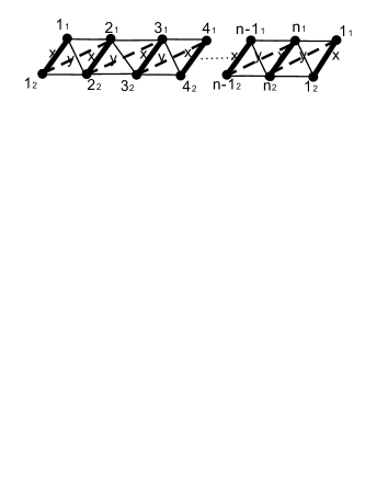
Figure 2: left panel: A chain of tetrahedrons on a torus. Right panel: unwind the torus to a periodic lattice. The thick lines carry $J_{x}$ while the dash lines carry $J_{y}$.

To well define an anyon, we generalize the single tetrahedron model to a chain model of tetrahedrons on a torus (Fig. 2). The model Hamiltonian is given by

$\displaystyle H_{\rm chain}=J_{x}\sum_{i=1}^{n}\sigma^{x}_{i_{1}}\sigma^{x}_{i_{2}}+J_{y}\sum_{i=1}^{n}\sigma^{y}_{i_{2}}\sigma^{y}_{i+1_{1}}$
$\displaystyle+\lambda\sum_{i=1}^{n}\sigma^{x}_{i_{1}}\sigma^{z}_{i_{2}}\sigma^{z}_{i+1_{1}}\sigma^{x}_{i+1_{2}}$ (14)
$\displaystyle+\kappa\sum_{i=1}^{n}(\sigma^{x}_{i_{1}}\sigma^{z}_{i_{2}}\sigma^{y}_{i+1_{1}}+\sigma^{y}_{i_{2}}\sigma^{z}_{i+1_{1}}\sigma^{x}_{i+1_{2}})$

with $n+1\equiv 1$. Only a half of triangular plaquette operators are conserved, which are $P=\{P_{2a-1}=P_{2a-1_{1}2a-1_{2}2a_{1}}=\sigma^{y}_{2a-1_{1}}\sigma^{z}_{2a-1_{2}}\sigma^{x}_{2a_{1}},P_{2a}=P_{2a-1_{1}2a_{1}2a_{2}}=\sigma^{y}_{2a-1_{2}}\sigma^{z}_{2a_{1}}\sigma^{x}_{2a_{2}}\}.$ The Hamiltonian can be diagonalized as

$\displaystyle H_{\rm chain}=-t\sum_{i=1}^{n}(d^{\dagger}_{i}d_{i+1}+d^{\dagger}_{i+1}d_{i})-\mu\sum_{i=1}^{n}d^{\dagger}_{i}d_{i}$
$\displaystyle+\sum_{i=1}^{n}(\Delta^{*}d_{i}d_{i+1}+\Delta d_{i+1}^{\dagger}d^{\dagger}_{i}),$ (15)

where $d_{i}=\frac{1}{2}(\psi_{i_{1}}-i\psi_{i_{2}})$ and the Majorna fermions are given by jw cn $\psi_{i_{1}}=\sigma^{x}_{i_{1}}\prod_{j<i}\sigma^{z}_{j_{1}}\sigma^{z}_{j_{1}},\psi_{i_{2}}=\sigma^{y}_{i_{2}}\sigma^{z}_{i_{1}}\prod_{j<i}\sigma^{z}_{j_{1}}\sigma^{z}_{j_{1}},~{}b_{i_{1}}=-\sigma^{y}_{i_{1}}\prod_{j<i}\sigma^{z}_{j_{1}}\sigma^{z}_{j_{1}},b_{i_{2}}=-\sigma^{x}_{i_{2}}\sigma^{z}_{i_{1}}\prod_{j<i}\sigma^{z}_{j_{1}}\sigma^{z}_{j_{1}},$ where Majorana fermions $b_{i}$ commute with $H_{\rm chain}$. Therefore, $b_{i}b_{j}\cdots|\rangle$ are degenerate states if $|\rangle$ is an eigen state. Since $[P,\psi_{i}]=0$ for all $i$ but not all $b_{i}$, the eigen values of $P$ for the vortex states $\eta_{i}=\frac{i}{\sqrt{2}}(b_{i}\tilde{\psi}_{p}-b_{j}b_{i}\tilde{\psi}_{p})$, $j\neq i$ are determined by $b_{i,j}$. Here $\tilde{\psi}_{p}$ are the linear combination of $\psi_{l}$ after diagonalizing $H_{\rm chain}$ as those in the single tetrahedron model. If $j$ is far from $i$, $\eta_{i}$ has only one minus $P$ near the $i$-th site. Then, $\eta_{i}$ is a well-defined single vortex operator and can be thought as a non-abelian anyon due to $\eta_{i}\eta_{i}=1+b_{j}$. There are $n$ such anyons which are degenerate. Each anyon brings a zero mode $b_{i}$ of Majorana fermion in its center iv kitaev .

Non-abelian braiding matrices Rewriting $\eta_{i}=\frac{1}{\sqrt{2}}(e_{i}-m_{i})$ with $e_{i}=ib_{i}\tilde{\psi}_{p}$ and $m_{i}=ib_{j}b_{i}\tilde{\psi}_{p}$, one has abelian fusuion rules $em\sim b$, $mb\sim e$, $eb\sim m$ and $e^{2}=m^{2}=b^{2}=1$. $e$ and $m$ are toric code mutual abelian anyons with degenerate energy. Thus, the Ising anyon is in fact the superposition of the toric code abelian anyons. This result has been recognized in refs. yusi ; wang but without involving the Hamiltonian. Therefore, the toric code braiding matrices determine the non-abelian braiding matrices of $\eta_{i}$ wang , which are Ising-like braiding matrices

$$R^{bb}_{1}=-1,~{}(R^{\eta\eta}_{1})^{2}=1,~{}(R^{b\eta}_{\eta})^{2}=-1,~{}(R^{\eta\eta}_{b})^{2}=-1.$$

Missing of the complex phases $e^{-i\pi/8}$ in $R^{\eta\eta}_{1}$ and $e^{i\pi/8}$ in $R^{\eta\eta}_{b}$ is because $R=R^{\dagger}$ for the toric code anyons wang . A framing therefore is needed lw . We do not intend to propose a framing and ancillary qubits to implement the non-trivial chirality but refer to Wootton et al wang .

In conclusions, we presented a simple model in which there are a set of vortices obeying non-abelian fusion rules which were explicitly illustrated in an elementary way without using deep mathematical tools. Finally, we generalized the single tetrahedron model to a chain model of tetrahedrons on a torus and showed that the non-abelian vortices defined in the single tetrahedron model become well-defined non-abelian anyons.

This work was supported in part by the national natural science foundation of China, the national program for basic research of MOST of China and a fund from CAS.

References

  • (1) A. Kitaev, Ann. Phys. 303, 2(2003).
  • (2) A. Kitaev, Ann. Phys. 321, 2(2006).
  • (3) C. Nayak, S. H. Simon, A. Stern, M. Freedman and S. Das Sarma, Rev. Mod. Phys. 80, 1083 (2008).
  • (4) M. A. Levin and X.-G. Wen, Phys. Rev. B 71, 045110 (2005)
  • (5) Y.-J. Han, R. Raussendorf and L.-M. Duan, Phys. Rev. Lett. 98, 150404 (2007). C. -Y. Lu, W. -B. Gao, O. Gühne, X. -Q. Zhou, Z. -B. Chen, and J. -W. Pan, arXiv:0710.0278. J. K. Pachos, W. Wieczorek, C. Schmid, N. Kiesel, R. Pohlner, and H. Weinfurter, arXiv:0710.0895. L. Jiang, G. K. Brennen, A. V. Gorshkov, K. Hammerer, M. Hafezi, E. Demler, M. D. Lukin, and P. Zoller, Nature Physics 4, 482 (2008). J. -F. Du,. J. Zhu, M. -G. Hu, and J. -L. Chen, arXiv:0712.2694. M. Aguado, G. K. Brennen, F. Verstraete, and J. I. Cirac, arXiv:0802.3163. B. Paredes and I. Bloch, arXiv:0711.3796. S. Dusuel, K. P. Schmidt, J. Vidal, Phys. Rev. Lett. 100, 177204 (2008).
  • (6) Yue Yu and Ziqiang Wang, arXiv: 0708.0631, to appear in Euro. Phys. Lett.
  • (7) H. Yao, S. C. Zhang, and S. A. Kivelson, arXiv: 0810.5347.
  • (8) C. J. Wu, D. Arovas, and H. -H. Hung, arXiv: 0811.1380.
  • (9) V. Lahtinen, G. Kells, A. Carollo, T. Stitt, J. Vala and J. K. Pachos, Ann. of Phys. 323, 2286 (2008).
  • (10) H. D. Chen and Z. Nussinov, J. Phys. A 41, 075001 (2008).
  • (11) Yue Yu and Tieyan Si, arXiv:0804.0483.
  • (12) J. R. Wootton, V. Lahtinen , Z. Wang, J. K. Pachos, Phys. Rev. B 78, 161102(R) (2008).
  • (13) D. A. Ivanov, Phys. Rev. Lett. 86, 268 (2001).
  • (14) H. Yao and S. A. Kivelson, Phys. Rev. Lett. 99, 247203 (2007).
  • (15) X. Y. Feng, G. M. Zhang, and T. Xiang, Phys. Rev. Lett. 98, 087204 (2007). H. D. Chen and J. P. Hu, Phys. Rev. B 76, 193101 (2007).