Revealing the fastest component of the DG Tau outflow through X-rays

Abstract

Context. Some T Tauri stars show a peculiar X-ray spectrum that can be modelled by two components with different absorbing column densities.

Aims. We seek to explain the soft X-ray component in DG Tau, the best studied of these sources, with an outflow model, taking observations at other wavelengths into consideration.

Methods. We constrain the outflow properties through spectral fitting and employ simple semi-analytical formulae to describe properties of a shock wave that heats up the X-ray emitting region.

Results. The X-ray emission is consistent with its arising from the fastest and innermost component of the optically detected outflow. Only a small fraction of the total mass loss is required for this X-ray emitting component. Our favoured model requires shock velocities between 400 and 500 km s^-1. For a density $>10^{5}$ cm^-3 all dimensions of the shock cooling zone are only a few AU, so even in optical observations this cannot be resolved.

Conclusions. This X-ray emission mechanism in outflows may also operate in other, less absorbed T Tauri stars, in addition to corona and accretion spots.

1 Introduction

Jets and outflows seem to be a natural consequence of disc accretion, as they are common phenomena in star formation. Jets are an especially active area of study at present. Their innermost region is particularly interesting because it arises from the deepest in the potential well and thus probes the conditions there, which cannot be resolved by direct imaging. This innermost region is crucial for our understanding of jet launching and collimation. We need to constrain the different theoretical models of stellar winds (Kwan & Tademaru 1988; Matt & Pudritz 2005), X-winds (Shu et al. 1994) and disc winds (Blandford & Payne 1982; Anderson et al. 2005) to produce reliable estimates of the associated angular momentum loss from the disc and possibly the star. This spin-down is needed to explain the slow rotation of accreting classical T Tauri stars (CTTS).

CTTS also have long been known as copious emitters of X-rays (Feigelson & Montmerle 1999), and we now recognise that multiple emission mechanisms contribute to the observed radiation. Studies of large statistical samples clearly show a coronal component, which occasionally breaks out in hard X-ray flares (Preibisch et al. 2005; Stelzer et al. 2007). Additionally a hot spot on the stellar surface heated by ongoing accretion contributes (Günther et al. 2007). It shows up in X-ray line ratios originating in high-density regions, much denser than any corona (Kastner et al. 2002; Stelzer & Schmitt 2004; Schmitt et al. 2005; Günther et al. 2006; Argiroffi et al. 2007). There is relatively recent evidence of X-rays from the outflows themselves, starting with HH 2 (Pravdo et al. 2001) and HH 154 (Favata et al. 2002; Bally et al. 2003; Favata et al. 2006). X-rays very likely trace the fastest shocks in the jets. The first spatially extended X-ray emission of a CTTS jet was found using Chandra by Güdel et al. (2005, 2008) in DG Tau. This star shows a spatially resolved, soft emission extending out to 5″. It is not compatible with a point source origin, and Güdel et al. (2008, hereafter GS08) model it by a combination of a linear source plus a Gaussian of $\approx 140$ AU diameter at the maximum distance to the star. Also, Güdel et al. (2007) find unusual spectral shapes in some CTTS distinguishing these so-called TAX (two absorber X-ray) sources from most other CTTS. Their spectra can be fitted well with a highly absorbed hard component and a much less absorbed soft component. They suggest that the marginally resolved soft excess is emission from the base of the jet (see also Schneider & Schmitt 2008). In this paper we develop this picture further in order to use the X-rays as a probe of the innermost, fastest outflow and to constrain the jet’s spatial extent and mass outflow rate. This idea is supported by the finding of Schneider & Schmitt (2008) that there is a small but significant spatial offset between the soft and the hard central components in DG Tau, so even the central component is marginally resolved.

We focus specifically on DG Tau, since the source is studied at many wavelengths, especially the stronger jet to the SW, but much less information is available for the fainter counter-jet to the NE. In the optical the jet has been imaged with HST/STIS several times, revealing not only jet rotation (Coffey et al. 2007), but also the presence of components with different velocities in the approaching jet with up to 600 km s^-1 (Bacciotti et al. 2000), after correcting for projection effects.

Based on analysis of forbidden lines, it was inferred that the jet density rapidly falls off with increasing distance from the star (Lavalley-Fouquet et al. 2000; Bacciotti et al. 2000). The jet extends to 0.5 pc as HH 702 (McGroarty et al. 2007), where shock-excited knots are clearly seen, but also closer to the star there has to be a heating source to sustain the jet emission. Heating by ambient shocks within the material itself is a good candidate. Takami et al. (2004) found a cool and slow molecular wind with an opening angle near $90\deg$, which surrounds the faster and hotter atomic outflow (see also Beck et al. 2008).

Raga et al. (2001) presented a 3D hydrodynamical simulation of the DG Tau jet. They assume a sinusoidal velocity variation and precession. The precession broadens up the working surfaces in an otherwise well-collimated beam and produces several shocks where the faster material catches up with the previously ejected slower matter. In this model the density decreases naturally with the distance to the stellar source.

In this paper we examine the emission measure, column density and temperature of the X-ray emitting region through spectral fitting (Sect. 2) and interpret the soft component as a tracer of the fastest component of the outflow (Sect. 3). We then discuss constraints from other wavelength bands and their implication for the outflow origin in Sect. 4. We present our conclusions in Sect. 5 and give a short summary in Sect. 6.

2 X-ray observations

We rely on the X-ray data presented by GS08, consisting of a 40 ks XMM-Newton observation (ObsID 0203540201) and four Chandra exposures (ObsIDs 4487, 6409, 7247 and 7246), which sum up to 90 ks observation time. We retrieved this data from the archives, reduced it using standard SAS and CIAO tasks, and analyse it in XSPEC. Because of the low count rate we merge all available Chandra data. GS08 show that the error bars on the fitted values overlap between the four exposures for the soft component. The luminosity in the hard component varies by a factor of three, but the other parameters are compatible. Since we are most interested in modelling the soft component, variations in the luminosity and temperature of the hard component are not important here. We simultaneously fit the merged Chandra and the XMM-Newton data with two thermal components with individual absorption. We keep the parameters for Chandra and XMM-Newton coupled in the soft component and leave the temperature and normalisation between the hard components free, because it is observed to be much stronger in the XMM-Newton observation due to intrinsic variability. As an illustration we show the data recorded by the EPIC/PN camera which covers the broadest energy range in Fig. 1. As black and red/grey lines we show two fits to the soft components with different temperatures. The fits shown use solar abundances according to Grevesse & Sauval (1998).

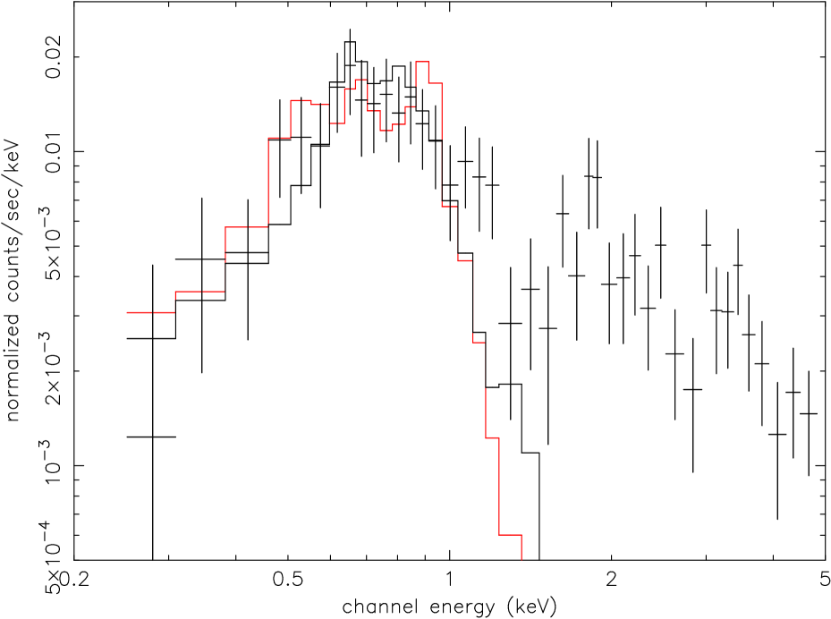
Figure 1: XMM-Newton EPIC/PN data of DG Tau. Overplotted are the contributions by the soft component for two different scenarios: $\textnormal{k}T=0.3$ keV ( $N_{\mathrm{H}}=2.3\times 10^{21}$ cm^-2; black line) and $\textnormal{k}T=0.08$ keV ($N_{\mathrm{H}}=11\times 10^{21}$ cm^-2; red/grey line).

Due to the low count numbers, the statistical uncertainties are large. In Fig. 1 the black line shows a model with $\textnormal{k}T=0.3$ keV and moderate absorption, very similar to that presented in GS08. However, a model with a much cooler temperature ($\textnormal{k}T=0.08$ keV), higher emission measure and larger absorbing column density reproduces the data nearly as well, as illustrated by the red/grey line in the figure. Thus, for the soft component, there is an ambiguity that makes it difficult to precisely determine the temperature, emission measure, and absorption column.

To quantify this, we have run a grid of models, keeping all parameters for the hard component fixed and leaving the cool component’s volume emission measure (VEM hereafter), temperature and absorption column density free. The resulting $\chi^{2}$-distribution is shown in Fig. 2. At the 99.95 % confidence level the distribution ranges over ten orders of magnitude in emission measure and one order of magnitude in temperature, following a narrow valley in Temperature–VEM space. The most likely temperature region is 0.2-0.4 keV with a second region within the 99 % confidence contour around 0.08 keV. The secondary peak around 0.08 keV is caused mostly by Chandra data; it does not appear in a fit to the data from XMM-Newton, which is more sensitive to low energy X-rays than Chandra.

We verified that the position of this valley in $\chi^{2}$-space does not change if the parameters of the hard component are left free. We fit the thermal emission with two APEC models. When using MEKAL, the minimum $\chi^{2}$-valley is in the same place, but the absolute minimum $\chi^{2}$ model is shifted to lower energies by up to 0.05 keV along the valley. We regard this as an estimate for the systematic uncertainty in the fit process.

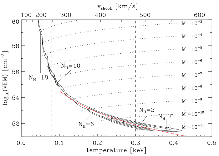
Figure 2: This shows confidence contours (at 68 %, 90 %, 99 % and 99.95 % confidence level) fitting the VEM and the temperature of the soft component. The parameters in the hard component are held fixed. Assuming a simple shock model (see text for details) the shock velocity is given on the upper horizontal axis and mass loss rates in M_☉ yr^-1 are marked in dotted lines in the plot. For some models absorbing column densities $N_{\mathrm{H}}$ are given in units of $10^{21}$ cm^-2. The temperatures of the two models shown in Fig. 1 are marked with dashed lines. Our fit from Eq. 1 is indicated with a red/grey line.

Due to this and the ambiguity in fitting the temperature and VEM of the soft component, rather than taking the formal minimum $\chi^{2}$ model, we consider a range of parameter space that is statistically allowed by the observations. Future observations will be needed to pin down more precise values. Thus, we fit a simple power-law to the minimum $\chi^{2}$-valley of figure 2. This gives

$$\frac{\mathrm{VEM}}{10^{52}\mathrm{cm}^{-3}}\approx 0.45\cdot\left(\frac{0.33\textnormal{ keV}}{\mathrm{k}T}\right)^{5.5}.$$ (1)

The emission measure of the minimum $\chi^{2}$-valley deviates less than a factor of 2 from equation (1) in the energy range 0.1-0.4 keV (Fig. 2). We will use this relationship in the following section.

To get a handle on the physical conditions in the emitting region further constraints are needed. The fact that the central component of the soft emission does not deviate significantly from a point source (Schneider & Schmitt 2008), gives an upper limit on the emitting volume and therefore a lower limit on the density. Its size should be less than 1″, corresponding to 140 AU at the distance of DG Tau. At the same time Schneider & Schmitt (2008) found the soft component to be significantly offset from the hard component at the stellar position by about 30 AU to the SW, the direction of the X-ray emitting, approaching jet.

3 A wind model

Figure 3: Sketch of the geometry. The flow launched from the region closest to the star travels with the highest velocity, and internal shocks in the flow there can reach the highest temperatures.

We use a simple, analytical model for the outflow. We discuss the observations giving rise to this model in detail in Sect. 4.3. Those observations indicate a collimated inner jet, which moves relatively fast. It is surrounded by slower and consecutively cooler components (e.g. Bacciotti et al. 2000, see Sect. 4.3 for more references). This situation – resembling the layers of an onion – is sketched in Fig. 3. The outer wind is launched from the disc whereas the origin of the inner jets could be either the inner disc region or the star itself. Disc winds are launched at a temperatures of $\sim 10^{4}$ K or much less (Ardila et al. 2002; Herczeg et al. 2006). Stellar winds, even if launched at coronal temperatures, will cool adiabatically, and the radiative cooling time can also be very short (Matt & Pudritz 2007). Therefore, beyond several tens of stellar radii, we expect all components of the outflow to be too cool to emit X-rays. The outer layer contains molecular hydrogen and radiates predominantly in the IR; the more collimated and faster flows can be observed in the optical.

Raga et al. (2001) modelled successfully the optical observations with a jet model using a time-variable outflow speed. This gives rise to strong shocks, when faster gas catches up with previous ejecta. We assume that in the innermost outflow region the velocity of the flow is high enough to heat the post-shock material to X-ray emitting temperatures. The shock forms sufficiently far from the star that the flow is collimated.

Using the strong shock conditions we can transform the thermal energy k$T$, where k is Boltzmann’s constant and $T$ is the temperature, into the pre-shock velocity in the shock rest frame $v_{\mathrm{shock}}$:

$$\left(\frac{v_{\mathrm{shock}}}{500\textnormal{ km s}^{-1}}\right)^{2}\approx\frac{\textnormal{k}T}{0.33\textnormal{ keV}}\;.$$ (2)

This velocity is given on the upper horizontal axis in Fig. 2. We emphasise that, in the case of a travelling shock wave, the pre-shock gas velocity is the sum of $v_{\mathrm{shock}}$ and the motion of the shock front. Raga et al. (2002) provided a semi-analytical formulation for estimating the cooling length of gas heated in fast shocks ($\Delta v\ga 200$ km/s). We checked this analytic relation with more detailed simulations of the shock cooling zone using our own code (Günther et al. 2007) and found that they agree within a factor of a few. Thus, for the semi-analytic treatment here, we will use the formula of Raga et al. (2002), which can be written

$$d_{\mathrm{cool}}\approx 20.9\mathrm{AU}\left(\frac{10^{5}\mathrm{cm}^{-3}}{n_{0}}\right)\left(\frac{v_{\mathrm{shock}}}{500\textnormal{ km s}^{-1}}\right)^{4.5},$$ (3)

where $n_{0}$ is the pre-shock particle number density, equal to a quarter of the post-shock number density $n$ in the strong shock approximation.

We assume an idealised cylindrical geometry for the post-shock flow, where the length of the cylinder is $d_{\mathrm{cool}}$. The mass flow rate $\dot{M}_{\rm shock}$ through the shock front with area $A$ is then given by

$$\dot{M}_{\rm shock} = Av_{\mathrm{shock}}\rho_{0},$$ (4)

where $\rho_{0}=\mu m_{\mathrm{H}}n_{\mathrm{ion}_{0}}$ is the pre-shock mass density of the flow, $n_{\mathrm{ion}_{0}}$ is the initial number density of heavy particles, i.e. atoms and ions, $\mu$ the mean relative ion particle weight, and $m_{\mathrm{H}}$ the mass of hydrogen. Assuming solar abundances, we adopt $\mu=1.26$. It is worth noting that $\dot{M}_{\rm shock}$ is less than the total mass loss rate in the flow, since $v_{\mathrm{shock}}$ is measured in the rest frame of the shock, and shocks in these systems are observed to travel at speeds of tens to hundreds of km s^-1.

The area of the shock can be determined from

$$A=\pi R^{2}={\mathrm{Volume}\over d_{\mathrm{cool}}}={VEM\over n_{\mathrm{e}}n_{\mathrm{ion}}d_{\mathrm{cool}}},$$ (5)

where $n_{\mathrm{e}}$ and $n_{\mathrm{ion}}$ are the post-shock electron and ion number density. Combing Eqs. 2–5, and assuming $n_{\mathrm{ion}}=4n_{\mathrm{ion}_{0}}=0.83n_{\mathrm{e}}$, the mass flow rate can be written

$$\dot{M}_{\rm shock} \approx 2.7\cdot 10^{-11}\frac{M_{\sun}}{\textnormal{yr}}\left(\frac{VEM}{10^{52}\textnormal{ cm}^{-3}}\right)\left(\frac{0.33\textnormal{ keV}}{\textnormal{k}T}\right)^{1.75}\;.$$ (6)

It is convenient that, by adopting a simple formula for the cooling length (Eq. 3) and a simple shock geometry, the determination of the mass loss rate is independent of the density of the flow.

We can now apply this specifically to the soft X-ray component of DG Tau. By combining the observed relationship of Eq. 1 with Eq. 6, one obtains

$$\dot{M}_{\rm shock} \approx 1.2\times 10^{-11}\frac{M_{\sun}}{\textnormal{yr}}\left(\frac{0.33\textnormal{ keV}}{\textnormal{k}T}\right)^{7.25},$$ (7)

or, using equation (2),

$$\dot{M}_{\rm shock} \approx 1.2\times 10^{-11}\frac{M_{\sun}}{\textnormal{yr}}\left(\frac{500\textnormal{ km s}^{-1}}{v_{\mathrm{shock}}}\right)^{14.5}.$$ (8)

These formulae indicate that the mass loss rate required to explain the observed soft X-rays has a very steep dependence on the observed temperature. It is clear that a better determination of the mass loss rate requires a more precise temperature measurement. In Fig. 2 lines of constant mass loss rate are marked as dotted lines according to Eq. 6. Over the full length of the confidence contour the mass loss varies by ten orders of magnitude.

We now look at the physical size of the shock region, $R$, which is the radius of the base of the emitting cylinder of shocked gas. From Eqs. (2), (3) and (5), we can solve for the radius (in AU),

$$R \approx 0.97\left(\frac{10^{5}\mathrm{cm}^{-3}}{n}\right)^{0.5}\left(\frac{VEM}{10^{52}\textnormal{ cm}^{-3}}\right)^{0.5}\left(\frac{0.33\mathrm{keV}}{\mathrm{k}T}\right)^{1.125},$$ (9)

and using the observed relationship for DG Tau (Eq. 1),

$$R \approx 0.65\textnormal{ AU}\left(\frac{10^{5}\mathrm{cm}^{-3}}{n}\right)^{0.5}\left(\frac{0.33\mathrm{keV}}{\mathrm{k}T}\right)^{3.875}.$$ (10)

In Fig. 4 the confidence contours for the lower mass loss rates are shown as functions of the radius of the shock at the cylinder base and the cooling length assuming a density of $n_{\mathrm{ion}}=10^{5}$ cm^-3 as motivated from the optical observations. For other densites the scalings are $R\sim\sqrt{\frac{1}{n}}$ (Eq. 9) and $d_{\mathrm{cool}}\sim\frac{1}{n}$ (Eq. 3).

Figure 4: Confidence contours (at 68 %, 90 % and 99 % confidence level) are shown for the parameters radius $R$ and shock velocity $v_{\mathrm{shock}}$ for the case of a cylindrical cooling zone at a fixed density of $n=10^{5}$ cm^-3. Dotted lines mark the mass loss rates in M_☉ yr^-1.

4 Discussion

In this section we will use the formulas and condition derived above to place limits on the physical mechanism producing the observed X-ray radiation.

4.1 Elemental abundance

The signal-to-noise ratio is not sufficient to fit elemental abundances, so we performed additional fits with the abundances found by Scelsi et al. (2007) for the Taurus molecular cloud. As usual there is a strong degeneracy between emission measure and metallicity. On average reduced abundances can be compensated for by a larger emission measure. Changes in the composition, that is particularly the Ne/O and Ne/Fe ratio, lead to different thermal structures. The confidence contours for fits with the abundances from Scelsi et al. (2007) follow the same valley in $\chi^{2}$-space, but are displaced about 0.07 keV to higher energies. Models below 0.27 keV are excluded on the 99% confidence level.

It is not clear, however, if the coronal abundance is applicable to the jet, since the launching region of the X-ray emitting, fast jet component is unknown.

4.2 Limits on the size of the shock

Figure 2 shows two distinct regions of the parameter space within the 99% confidence level. That region in the upper left corner corresponds to a scenario of a large emission measure, which is heavily absorbed. The temperature is only around 0.08 keV and therefore the $v_{\mathrm{shock}}\approx 250$ km s^-1. As an upper limit we assume a density of $10^{5}$ cm^-3 (see next section). The cooling length according to Eq. 3 should be about 1 AU. In a simple cylindrical geometry the volume emission measure, transformed to a cylindrical radius with Eq. 9, requires a base shock with a radius of 1000 AU, but this would appear as an extended source, which is not observed for the central component (GS08, Schneider & Schmitt 2008). Only a density above $10^{7}$ cm^-3 could push all shock dimensions below $\approx 100$ AU, so they appear as point source in the X-ray observation.

We deem this unreasonably high, also the low energy region is excluded in fits to the XMM-Newton data alone or in models with different – but reasonable – abundances, so we concentrate on the less absorbed case with a higher $v_{\mathrm{shock}}$ in Fig. 4. This parameter region can be realised with emission from the inner component of the jet only.

4.3 Limits placed by other observations

Observations with the HST allow to spatially resolve the outflow of DG Tau far below 1″ from the central source. The forbidden optical lines observed place density constraints. Bacciotti et al. (2000) conducted seven exposures with a long slit parallel to DG Tau’s outflow in H$\alpha$ and forbidden optical lines. They analyse the line shift within 0$\aas@@fstack{\prime\prime}$5 from the star and find that the faster moving gas is more confined towards the central axis. The emission of gas faster than 200 km s^-1 is mostly confined to the inner slit, corresponding to a cylinder of radius 15 AU or less. Comparison of intensity maps in [O i], [N ii] and [S ii] leads them to conclude that the number density in the fast gas is higher than $10^{4}$ cm^-3 (the line ratios are not sensitive to densities above this value). The lower velocity emission occupies a larger area and originates in regions of lower densities of the order $10^{3}-10^{4}$ cm^-3. So, the inner, dense and fast components seem to be surrounded by slower and less dense outflows, maybe continuously down to a cool wind observed in H₂ with an opening angle of 90°(Takami et al. 2004). Consistent density estimates of $10^{5}-10^{6}$ cm^-3 at distances less than 0$\aas@@fstack{\prime\prime}$5, deprojected to $\approx 100$ AU, were obtained by Lavalley-Fouquet et al. (2000). Strictly speaking, their line ratios give only lower limits on the density for the fastest innermost components, too, but in any case the outer layers do not contribute significantly to the X-ray radiation.

From the total line intensity Lavalley et al. (1997) estimate a total mass loss rate of $6.5\cdot 10^{-6}$ M_☉ yr^-1 if the gas is heated by shocks. With somewhat similar assumption Hartigan et al. (1995) obtain $3\cdot 10^{-7}$ M_☉ yr^-1. At a distance of 1$\aas@@fstack{\prime\prime}$2 from the central source Lavalley-Fouquet et al. (2000) estimate a mass loss rate of $1.4\cdot 10^{-8}$ M_☉ yr^-1. This evidence again favours the lower corner in Fig. 2, shown in more detail in Fig. 4.

In optical and IR line emission is detected blue-shifted up to deprojected velocities of 600 km s^-1 (Lavalley-Fouquet et al. 2000; Bacciotti et al. 2000; Pyo et al. 2003). An analysis of data covering more than a decade by Pyo et al. (2003) indicates that the knots in the outflow move with a common proper motion of 0$\aas@@fstack{\prime\prime}$28 yr^-1, which translates into a deprojected velocity of 300 km s^-1.

4.4 The shocked gas component

As shown in Sect. 4.2 the X-ray emission is unlikely to originate in the slowly moving components of the outflow. This leaves the innermost component as the probable emission origin. Unrealistically high densities are needed to produce an emission measure of $10^{56}$ cm^-3 for low shock speeds, so we favour a scenario where a strong shock with $v_{\mathrm{shock}}>400$ km s^-1 heats up a relatively small component of the jet. In this case the emission measure is much smaller, so the required mass flux to power this emission is several orders of magnitude smaller than the total mass flux observed in the optical. The dotted lines in Fig. 4 show the mass loss depending on $v_{\mathrm{shock}}$. Taking into account the observed proper motion of the knots, the gas velocities of e.g. Bacciotti et al. (2000) are too low to explain the X-ray spectrum. Because less than $10^{-4}$ of the total flow has to reach the highest velocity to produce the X-rays, this small component was possibly not detected in the optical observations. In scenarios with standing (collimation shock) instead of travelling shock waves the innermost component is fast enough to explain the observed emission easily.

After passing through the X-ray shock the material quickly radiates away its energy and cools down. Figure 4 shows all dimensions, the cooling length and the radius of the cylinder, to be small, therefore, they are not expected to be resolved in the HST observations. The X-ray emitting shock is only a small disturbance and within a few AU the material has cooled down again to match the temperatures of the surrounding gas. The shocks we discuss here cannot be resolved in images directly, so only a spectral analysis can help to further refine the model.

4.5 Formation of the shock front

Although the Chandra observations are separated by nearly two years, no evidence of motion has been detected (Schneider & Schmitt 2008), but given the size of the error circles a velocity $v_{\mathrm{front}}$ of the shock front of 100 km s^-1 in the stellar rest frame cannot be excluded. In this case the wind mass loss rate $\dot{M}_{\mathrm{wind}}$ has to be calculated using the sum of $v_{\mathrm{front}}$ and $v_{\mathrm{shock}}$:

$$\dot{M}_{\mathrm{wind}}=\frac{v_{\mathrm{front}}+v_{\mathrm{shock}}}{v_{\mathrm{shock}}}\dot{M}_{\mathrm{shock}}$$ (11)

If these knots represent internal working surfaces the associated $v_{\mathrm{shock}}$ is the difference between the gas motion and the proper motion about 300 km s^-1 for the knots. This by itself is not sufficient to power X-ray emission in the high temperature regime of Fig. 2. The knots seem to be launched irregularly, and the later Chandra observations could possibly probe a different knot than the earlier observations. A relatively slow shock speed of 400 km s^-1 corresponding to a total mass loss rate of roughly $3\times 10^{-10}$ M_☉ yr^-1 (Fig. 4) is then just compatible with the highest optically detected outflow velocities. One more scenario can be postulated: Instead of a single (stationary or moving) shock front a higher number of small internal shocks could produce the same X-ray signature. Each of these “shocklets” would not show up in the optical observations, because radius and cooling lengths were far below the current resolution limit. This requires a clumpy outflow, where the jet contains a higher number of little knots surrounded by the optically detected fast wind. Our calculated shock area and cooling volume then represents the sum of all individual shocks. This argument is also valid, if the matter passes through multiple shock fronts and is reheated several times. The calculated mass flux rate still represents the summed flow of matter through all shock fronts, but it needs to be divided by the number of shocks to obtain the mass loss rate from the star. The optical observations discussed in Sect. 4.3 do not resolve the postulated X-ray shock front, but the optically resolved shock fronts seem to emerge separated by 150 AU (A1 and A2 in Bacciotti et al. (2000)), so it appears reasonable that the X-rays may originate in a single shock front within 50 AU of the central star.

From our modelling there is no clear distinction between a stationary emission region as provided by a collimation shock or a moving knot. Only further observations with a longer time baseline can clarify this point. This is possible well within Chandra’s lifetime.

4.6 The outflow origin

The X-rays originate in the innermost and fastest component, which may originate from the innermost part of the disc or from the star itself. Matt & Pudritz (2007) showed that a T Tauri stellar wind with $\dot{M}_{\rm wind}\ga 10^{-11}$ M_⊙ yr^-1 cannot be coronally driven, but Alfvén wave driving may be possible (Cranmer 2008). The spin rate of DG Tau makes centrifugal launching of a stellar wind unlikely, whereas the outer layers with lower flow velocities are most likely centrifugally launched from the inner disc regions (Bacciotti et al. 2002; Anderson et al. 2003).

4.7 Relation to extended X-ray jet of DG Tau

The material heats up while passing through the shock front and we could show that the cooling length is very small compared to spatial extend of the jet. While cooling, the jet looses energy, so the strength of the shock fronts decreases, their velocity jump diminishes with time. In their paper de Colle & Raga (2006) show this in magneto-hydrodynamical models with a time variable ejection velocity leading to travelling shock fronts. Additionally, according to the optical observations, the density decreases with the distance from the star. Therefore later heating events are less luminous, so the resolved source at 5″ is weaker. Although the resolved shock is a spatially extended source, this does not necessarily require multiple heating events between 2″ and 5″, because the cooling length increases dramatically for low densities (GS08).

If the cause of the shock is a collision with slower, previously ejected matter we can expect this to happen more than once. In this picture the knot of X-ray emission at 5″ is caused by matter catching up with an older ejection event. GS08 convincingly show that knots even further out are far too faint in X-rays to be detected.

5 Conclusion

The soft X-ray emission of DG Tau is consistent with our model of a shock in the outflow. The cause of the shock is not yet clear, but future observations can reveal if the position of the shock front is stationary. In this case it is likely caused by the collimation of the wind into the jet. If, on the other hand, the shock front moves, then we can take this as indication that the outflow ejection velocity is highly variable. In both cases only the fastest components of the optically detected outflow provide sufficient energy to power the X-ray emission. Possible future grating observations could greatly improve our estimate of the temperature in the emitting region and narrow down the range of possible shock velocities and therefore – via Fig. 4 – the mass loss rate.

DG Tau is an exceptional CTTS in the sense that its central component is so much absorbed that the origin of the soft emission cannot coincide with the star. This makes it an ideal case to search for alternative origins and our simple model successfully reproduces the observation. On other CTTS, most notably TW Hya, detailed models of an accretion shock explain the X-rays production very well (Günther et al. 2007). It seems possible, that TW Hya also has a weak contribution from wind shocks to its emission, but its outflows are much weaker than those of DG Tau, so the X-rays would be submerged in the stellar emission. Next to accretion and coronal activity the wind shocks, as discussed in this article, may hold as the third emission mechanism of soft X-rays, although it is difficult to disentangle the contributions except in special cases.

6 Summary

In the X-ray spectrum of DG Tau there is a spatially only marginally resolved soft component. Because no grating information is available, the temperature is only poorly constrained and plasma models with a wide range of temperatures can reproduce the observations. The absorbing column density is negligible in the case of plasma with a thermal energy of $\textnormal{k}T=0.4$ keV and rises to $N_{\textnormal{H}}>10^{22}$ cm^-2 for $\textnormal{k}T=0.1$ keV. For this second scenario the fitted emission measure would be several orders of magnitude higher. We reject this solution because it is not stable to small changes of the fit parameters and requires physically unreasonable values for the density in the shock region.

The emission can be explained by a shock and its corresponding cooling zone in the innermost and fastest component of the optically detected outflow. For densities $>10^{5}$ cm^-3 this is consistent with all available optical observations. Compared to the larger structures seen in the forbidden optical lines, this X-ray cooling zone could be a relatively thin layer. Only a small fraction of the total mass loss is needed in the innermost layer in order to produce the observed luminosity.