Black and gray spatial optical solitons with Kerr-type nonlocal nonlinearity

Abstract

We develop one numerical method to compute black and gray solitons with Kerr-type nonlocal nonlinearity. As two examples of nonlocal cases, the gray soliton with exponentially decaying nonlocal response or with Gaussian nonlocal response are discussed. For such two nonlocal cases, the analytical form of the tails of nonlocal gray soliton is presented and the analytical relationship for the maximal transverse velocity of nonlocal gray soliton to the characteristic nonlocal length is obtained.

I Introduction

In present years spatial solitons with Kerr-type nonlocal nonlinearity have attracted a great amount of studies. It is indicated the nonlocality of the nonlinearity ensures the existence of stable multidimensional solitons1 ; 2 ; 3 ; 4 . The nonlocal bright spatial solitons have been experimentally observed in nematic liquid crystal5 ; 6 ; 7 and in the lead glass8 . The propagation and interaction properties of nonlocal bright/black solitons are greatly different from that of local solitons. For example, the dependent functions of the beam power and phase constant on the beam width for nonlocal bright solitons are very different from those for local bright solitons9 ; 10 ; 11 ; There exists higher order Hermite-Gaussian like (1+1) dimensional bright nonlocal solitons9 ; 10 ; 12 and Laguerre-Gaussian like (1+2) dimensional bright nonlocal solitons9 ; 11 ; 12 ; 13 ; 14 ; 15 ; Bright nonlocal solitons with $\pi$ phase difference attract rather repel each other12 ; 16 ; 17 ; 18 ; Nonlocal black solitons can attract each other and two black solitons can form a bound state19 ; 20 ; 21 . The nonlocal gray solitons also can form a bound state24 .

In this paper we present a numerical method to compute black and gray soliton solutions with Kerr-type nonlocal nonlinearity. This numerical method is a generalized version of the so called spectral renormalization method presented by M. J. Ablowitz and Z. H. Musslimani22 with which they compute the bright soliton solutions. Our numerical method can be easily generalized to compute a large family of gray soliton solutions with other type of nonlinearity. It is worth to note that Yaroslav V. Kartashov and Lluis Torner24 has rather successfully studied the nonlocal gray soliton with an exponential decaying nonlocal response in a different manner. They has revealed that the gray soliton velocity depends on the nonlocality degree and pointed out the maximal velocity of gray soliton monotonically decreases with the degree of nonlocality24 . In our paper, besides of the nonlocal case of an exponential decaying nonlocal response, the nonlocal case of Gaussian nonlocal response is also discussed. The analytical form of the tails of nonlocal gray soliton is presented. It is indicated that nonlocal gray solitons can have exponentially decaying tails or have exponentially decaying oscillatory tails. The analytical relationship for the maximal transverse velocity of nonlocal gray soliton to the characteristic nonlocal length is presented. It is indicated when the characteristic nonlocal length is less than some critical value, such maximal transverse velocity is a constant and equal to that of local gray soliton, otherwise such maximal velocity will decrease with the increasing of the characteristic nonlocal length. That mostly agrees with the results of reference[24] with slight but not trivial exception. It was said in reference[24] that such maximal velocity monotonically decreases with the characteristic nonlocal length. But as will be shown in our paper the maximal velocity does not vary with the characteristic nonlocal length when the characteristic nonlocal length is less than some critical value. Our paper poses a problem for such inconsistence.

II Numerical method to compute nonlocal gray solitons

The propagation of an (1+1) dimensional optical beam in Kerr-type nonlocal self-defocusing media can be described by this following (1+1) dimensional nonlocal nonlinear Schödinger equation(NNLSE)1 ; 2 ; 3 ; 4 ; 5 ; 6 ; 7 ; 8 ; 9 ; 10 ; 11 ; 12 ; 13 ; 14 ; 15 ; 16 ; 17 ; 18 ; 19 ; 20 ; 21

$$i{\partial u\over\partial z}+\frac{1}{2}{\partial^{2}u\over\partial x^{2}}-u\int R(x-\xi)|u(\xi,z)|^{2}d\xi=0,$$ (1)

where $u(x,z)$ is the complex amplitude envelop of the light beam, $|u(x,z)|^{2}$ is the light intensity, $x$ and $z$ are transverse and longitude coordinates respectively, $R(x)$, ($\int R(x)dx=1$) is the real symmetric nonlocal response function, and $n(x,z)=-\int R(x-\xi)|u(\xi,z)|^{2}d\xi$ is the light-induced perturbed refractive index. Note that not stated otherwise all integrals in this paper will extend over the whole x axis. When $R(x)=\delta(x)$, equation (1) will reduce to the local nonlinear Schödinger equation(NLSE)

$$i{\partial u\over\partial z}+\frac{1}{2}{\partial^{2}u\over\partial x^{2}}-|u|^{2}u=0,$$ (2)

which has black and gray soliton solutions23

$$u(x,z) =\psi(x)e^{i[\beta z+\phi(x)]}$$ (3a)

$$\psi(x) =\eta[1-B^{2}\rm{sech}^{2}(\eta Bx)]^{1/2}$$ (3b)

$$\beta =-{{1}\over{2}}\eta^{2}(3-B^{2})$$ (3c)

$$\phi(x) =\eta\sqrt{1-B^{2}}x+\arctan\left[{{B\tanh(\eta Bx)}\over{\sqrt{1-B^{2}}}}\right]$$ (3d)

It is easy to prove that $\psi(x)\xrightarrow{x\rightarrow+\infty}\eta$ and $\phi^{\prime}(x)\xrightarrow{x\rightarrow+\infty}\eta\sqrt{1-B^{2}}\equiv\mu$. So we have $\beta=-({{\mu^{2}}\over{2}}+\eta^{2})$ which, as will be shown, also applies to nonlocal gray soliton.

In this paper we numerically compute the black and gray soliton solutions of NNLSE (1) that take these following form

$$u(x,z)=\psi(x)e^{i\beta z+i\phi(x)}$$ (4a)

$$\psi^{*}(x)=\psi(x)~{}~{}~{}~{}~{}\lim_{x\rightarrow+\infty}\psi(x)=\eta>0$$ (4b)

$$\beta^{*}=\beta~{}~{}~{}~{}~{}~{}~{}~{}~{}~{}~{}~{}~{}~{}~{}\phi^{*}(x)=\phi(x)$$ (4c)

Substitution of Eq. (4a) into (1), we have an equation for $\psi(x)$ and $\phi(x)$. Since both the real and imaginary part of such resulting equation must vanish, we have

$$-\beta\psi+{{1}\over{2}}\psi^{\prime\prime}-{{1}\over{2}}(\phi^{\prime})^{2}\psi-\psi\int R(x-\xi)\psi^{2}(\xi)d\xi=0$$ (5)

$$2\phi^{\prime}\psi^{\prime}+\phi^{\prime\prime}\psi=0$$ (6)

From Eq. (6),we have ${{d}\over{dx}}(\psi^{2}\phi^{\prime})=0$, which results in $\psi^{2}\phi^{\prime}=\rm{const}$. We set this constant as $\mu\eta^{2}$, where $\mu^{*}=\mu$ is another constant. So we have

$$\phi^{\prime}={{\mu\eta^{2}}\over{\psi^{2}}}.$$ (7)

Since $\psi(x)\xrightarrow{x\rightarrow+\infty}\eta$ as assumed in Eq. (4b), from Eq. (7), we have $\phi^{\prime}(x)\xrightarrow{x\rightarrow+\infty}\mu$, which in turn results in $\phi(x)\xrightarrow{x\rightarrow+\infty}c+\mu x$, where $c$ is a constant. The phase jump through the soliton is defined as $2c$. Substituting Eq. (7) into (5), we get

$$-\beta\psi+{{1}\over{2}}\psi^{\prime\prime}-{{\mu^{2}\eta^{4}}\over{2\psi^{3}}}-\psi\int R(x-\xi)\psi^{2}(\xi)d\xi=0.$$ (8)

Since $\psi(x)\xrightarrow{x\rightarrow+\infty}\eta$ and $\int R(x)dx=1$, from Eq. (8), when $x\rightarrow+\infty$, we have $-\beta\eta-{{\mu^{2}\eta}\over{2}}-\eta^{3}=0$ that leads to

$$\beta=-\left({{\mu^{2}}\over{2}}+\eta^{2}\right),$$ (9)

and

$${{\mu^{2}+2\eta^{2}}\over{2}}\psi+{{\psi^{\prime\prime}}\over{2}}-{{\mu^{2}\eta^{4}}\over{2\psi^{3}}}-\psi\int R(x-\xi)\psi^{2}(\xi)d\xi=0.$$

So the gray soliton takes a form of $u(x,z)=\psi(x)\exp[-i({{\mu^{2}}\over{2}}+\eta^{2})z+i\phi(x)]$, where $\psi(x),\phi(x)$ satisfy Eqs. (II) and (7). It is easy to prove that the Galilean transformed solution

$$u_{1}(x,z) \equiv u(x+\mu z,z)e^{i(-\mu x-{{1}\over{2}}\mu^{2}z)}$$ (11)

$$=\psi(x+\mu z)e^{i[-\eta^{2}z+\phi(x+\mu z)-\mu(x+\mu z)]}$$

$$=\psi_{1}(x+\mu z)e^{-i\eta^{2}z},$$

where $\psi_{1}(x+\mu z)\equiv\psi(x+\mu z)e^{i[\phi(x+\mu z)-\mu(x+\mu z)]}$, also satisfies the NNLSE (1). Since $|u_{1}(x,z)|^{2}=|\psi_{1}(x+\mu z)|^{2}=\psi^{2}(x+\mu z)$, the gray soliton moves in velocity $-\mu$ with respect to the coordinate system. On the other hand, since $\psi(x)\xrightarrow{x\rightarrow+\infty}\eta$ and $\phi(x)\xrightarrow{x\rightarrow+\infty}c+\mu x$, from Eq. (11), we have $u_{1}(x,z)\xrightarrow{x\rightarrow+\infty}\eta e^{i(c-\eta^{2}z)}$, which implies the background of gray soliton is at rest with respect to the coordinate system. So the soliton $u_{1}(x,z)$ moves in transverse velocity $-\mu$ with respect to the background intensity of gray soliton. In this paper we simply refer $-\mu$ as the transverse velocity of the soliton.

Assuming $\psi(x)\xrightarrow{x\rightarrow-\infty}\eta^{\prime}$, from Eq. (II), we have $\eta^{\prime}=\pm\eta$. When $\mu\neq 0$,the term ${{\mu^{2}\eta^{4}}\over{2\psi^{3}}}$ requires $\psi(x)\neq 0$, which in turn requires $\eta^{\prime}=\eta$. So the case $\mu\neq 0$ corresponds to the gray solitons and $\psi(-x)=\psi(x)$, where we have set $x=0$ be the symmetric center.

We study the case $\mu\neq 0$ in this section and leave the case $\mu=0$ to be discussed in the next section. Let

$$\psi(x)=\eta-\chi(x),$$ (12)

where $\chi(-x)=\chi(x)$ and $\chi(x)\xrightarrow{x\rightarrow\pm\infty}0$. Then Eq. (II) turns into

$$-{{\mu^{2}}\over{2}}\chi-{{1}\over{2}}\chi^{\prime\prime}+{{\mu^{2}\eta}\over{2}}\cdot{{3\eta\chi^{2}-3\eta^{2}\chi-\chi^{3}}\over{(\eta-\chi)^{3}}}$$

$$~{}-(\eta-\chi)\int R(x-\xi)[\chi^{2}(\xi)-2\eta\chi(\xi)]d\xi=0.$$ (13)

We discrete the function $\chi(x)$ in $\chi_{j}=\chi\big{(}-h+(j-1)\triangle x\big{)}$, where $-h<x<h$ is the sample window, $\triangle x$ is the sample step and $1\leq j\leq n={{2h}\over{\triangle x}}+1$. Define the discrete Fourier transform (DFT) $\mathscr{F}$ by

$$\widetilde{\chi}_{j}=\mathscr{F}[\chi]_{j}=\sum_{k=1}^{n}\rm{F}_{jk}\chi_{k},$$ (14a)

$$\chi_{j}=\mathscr{F}^{-1}[\widetilde{\chi}]_{j}=\sum_{k=1}^{n}\rm{F}^{*}_{jk}\widetilde{\chi}_{k},$$ (14b)

where $\rm{F}_{jk}={{1}\over{\sqrt{n}}}\exp[i{{2\pi}\over{n}}(j-1)(k-1)]$. Performing the DFT on Eq. (II), we have

$$-{{\mu^{2}}\over{2}}\widetilde{\chi}_{j}+{{\Omega_{j}}\over{2}}\widetilde{\chi}_{j}+{{\mu^{2}\eta}\over{2}}\mathscr{F}\left[{{3\eta\chi^{2}-3\eta^{2}\chi-\chi^{3}}\over{(\eta-\chi)^{3}}}\right]_{j}$$

$$-\mathscr{F}\left[(\eta-\chi)\int R(x-\xi)[\chi^{2}(\xi)-2\eta\chi(\xi)]d\xi\right]_{j}=0,$$

where $\Omega_{j}=\left({{2\sin[{{\pi}\over{n}}(j-1)]}\over{\triangle x}}\right)^{2}$. Let

$$\chi(x)=\lambda\theta(x),$$ (16)

we have

$$-{{\mu^{2}}\over{2}}\widetilde{\theta}_{j}+{{\Omega_{j}}\over{2}}\widetilde{\theta}_{j}+{{\mu^{2}\eta}\over{2}}\mathscr{F}\left[{{3\lambda\eta\theta^{2}-3\eta^{2}\theta-\lambda^{2}\theta^{3}}\over{(\eta-\lambda\theta)^{3}}}\right]_{j}$$

$$-\mathscr{F}\left[(\eta-\lambda\theta)\int R(x-\xi)[\lambda\theta^{2}(\xi)-2\eta\theta(\xi)]d\xi\right]_{j}=0.$$

Projecting Eq. (II) onto $\widetilde{\theta}$, we obtain an equation for $\lambda$

$$~{}~{}\mathscr{A}_{\theta}(\lambda)$$

$$\equiv\sum_{j=1}^{n}\widetilde{\theta}_{j}^{*}\bigg{\{}-{{\mu^{2}}\over{2}}\widetilde{\theta}_{j}+{{\Omega_{j}}\over{2}}\widetilde{\theta}_{j}$$

$$+{{\mu^{2}\eta}\over{2}}\mathscr{F}\left[{{3\lambda\eta\theta^{2}-3\eta^{2}\theta-\lambda^{2}\theta^{3}}\over{(\eta-\lambda\theta)^{3}}}\right]_{j}$$

$$-\mathscr{F}\left[(\eta-\lambda\theta)\int R(x-\xi)[\lambda\theta^{2}(\xi)-2\eta\theta(\xi)]d\xi\right]_{j}\bigg{\}}$$

$$=0.$$ (18)

On the other hand, from Eq. (II), we get

$$\widetilde{\theta}_{j} ={{r\widetilde{\theta}_{j}+{{\mu^{2}}\over{2}}\widetilde{\theta}_{j}-{{\mu^{2}\eta}\over{2}}\mathscr{F}\left[{{3\lambda\eta\theta^{2}-3\eta^{2}\theta-\lambda^{2}\theta^{3}}\over{(\eta-\lambda\theta)^{3}}}\right]_{j}}\over{r+{{\Omega_{j}}\over{2}}}}$$ (19)

$$+{{\mathscr{F}\left[(\eta-\lambda\theta)\int R(x-\xi)[\lambda\theta^{2}(\xi)-2\eta\theta(\xi)]d\xi\right]_{j}}\over{r+{{\Omega_{j}}\over{2}}}}$$

$$\equiv\mathscr{D}_{\lambda}[\theta]_{j}$$

where $r$ is a positive constant.

We use Eqs. (II) and (19) to iteratively compute gray soliton solutions. For an initial function $\theta_{1}(x)$, e.g. a Gaussian function, from Eq. (II), we get $\lambda_{1}$ which satisfies the equation $\mathscr{A}_{\theta_{1}}(\lambda_{1})=0$. Then from Eq. (19) we get function $\widetilde{\theta}_{2}=\mathscr{D}_{\lambda_{1}}[\theta_{1}]$. For $m\geq 1$, we get the iteration scheme $\mathscr{A}_{\theta_{m}}(\lambda_{m})=0,\widetilde{\theta}_{m+1}=\mathscr{D}_{\lambda_{m}}[\theta_{m}]$. Perform the iteration until the convergence is achieved. Then we get $\psi(x)=\eta-\lambda\theta(x)$ and $\phi(x)=\int_{0}^{x}{{\mu\eta^{2}}\over{\psi^{2}(\xi)}}d\xi$.

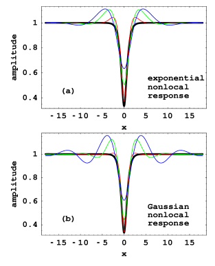
Figure 1: Amplitudes of gray soliton solutions with exponential nonlocal response (a) or with Gaussian nonlocal response (b). The parameters used are $\eta=1,\mu=1/3$ and black line corresponds to local case $w=0$, red line $w=1$, green line $w=3$ and blue line $w=5$ both for (a) and (b).

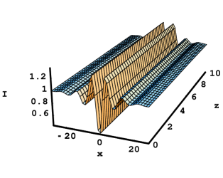
Figure 2: Numerical simulation of the gray soliton with Gaussian nonlocal response and with parameters $w=5,\eta=1,\mu=1/3$.

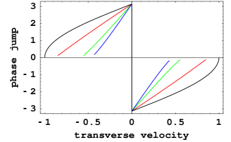
Figure 3: Phase jump through the nonlocal gray soliton with an exponential nonlocal response. Black line is the local case $w=0$; Red line $w=1$; Green line $w=3$; Blue line $w=5$.

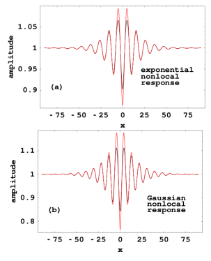
Figure 4: (a) Black line is the amplitude of gray soliton solution with exponential nonlocal response and with parameters $\eta=1,\mu=0.43,w=5$, and the red line is the fitting function $1-0.137\exp(-0.0753|x|)\cos(0.596|x|+0.055)$; (b) Gray soliton solution with Gaussian nonlocal response with parameters $\eta=1,\mu=0.4,w=5$ and the fitting function $1-0.238\exp(-0.0733|x|)\cos(0.713|x|+0.107)$.

As an example, we consider this following nonlocal case1 ; 2 ; 3 ; 4 ; 5 ; 6 ; 7 ; 10 ; 11 ; 16 ; 18 ; 21 ; 24

$$n-w^{2}{{d^{2}n}\over{dx^{2}}}=-|u|^{2},$$ (20)

which results in $n(x)=-\int{{1}\over{2w}}\exp(-{{|x-\xi|}\over{w}})|u(\xi)|^{2}d\xi$, where $R(x)={{1}\over{2w}}\exp(-{{|x|}\over{w}})$ is the exponential decaying nonlocal response function. In another example, we consider the Gaussian nonlocal response2 ; 3 ; 9 ; 10 ; 11 ; 14 ; 15 ; 17 ; 18 $R(x)={{1}\over{w\sqrt{\pi}}}\exp\left(-{{x^{2}}\over{w^{2}}}\right)$. For such two nonlocal cases, $w$ is referred as the characteristic nonlocal length. In Fig. (1) some nonlocal gray soliton solutions are shown. The numerical simulation result in Fig. (2) indicates the numerical nonlocal gray soliton solution obtained can describe the soliton state very well. The phase jump through the nonlocal gray soliton is shown in Fig. (3). As shown by Fig. (4) the nonlocal gray solitons can have exponentially decaying oscillatory tails for both the exponential nonlocal response case and the Gaussian nonlocal response case.

Now we investigate the form of the decaying tails of gray solitons. In case $|\chi(x)|\ll\eta$, to the leading order Eq. (II) can be linearized to

$$-2\mu^{2}\chi-{{1}\over{2}}\chi^{\prime\prime}+2\eta^{2}\int R(x-\xi)\chi(\xi)d\xi=0.$$ (21)

Since Eq. (21) is linear for $\chi(x)$, the superposition theorem applies.

For the exponential nonlocal response $R(x)={{1}\over{2w}}\exp(-{{|x|}\over{w}})$, Eq. (21) reduces to two coupled equations

$$-2\mu^{2}\chi-{{1}\over{2}}\chi^{\prime\prime}+2\eta^{2}f(x)=0,$$ (22a)

$$f(x)-w^{2}f^{\prime\prime}(x)=\chi(x).$$ (22b)

The solution of (22) can be assumed as

$$\chi(x)=\alpha\exp(\lambda x).$$ (23)

Substituting (23) into (22), we have

$$\chi^{\prime\prime}=4\left({{\eta^{2}}\over{1-\lambda^{2}w^{2}}}-\mu^{2}\right)\chi$$ (24)

The eigenvalue problem of the above equation provides an equation for $\lambda$

$$\lambda^{2}=4\left({{\eta^{2}}\over{1-\lambda^{2}w^{2}}}-\mu^{2}\right),$$ (25)

which results in

$$\lambda^{2}={{1-4\mu^{2}w^{2}-\sqrt{1+8\mu^{2}w^{2}+16\mu^{4}w^{4}-16\eta^{2}w^{2}}}\over{2w^{2}}}.$$ (26)

When $w\rightarrow 0$, from Eq. (26) to the leading order we have

$$\lambda^{2}=4(\eta^{2}-\mu^{2})(1+4\eta^{2}w^{2})$$ (27)

The roots of Eq. (26) are

$$\lambda=\pm(\lambda_{1}+i\lambda_{2}),$$ (28)

where

$$\lambda_{1}=\sqrt{{{1-4w^{2}\mu^{2}+4w\sqrt{\eta^{2}-\mu^{2}}}\over{4w^{2}}}},$$ (29)

$$\lambda_{2}=\sqrt{{{-1+4w^{2}\mu^{2}+4w\sqrt{\eta^{2}-\mu^{2}}}\over{4w^{2}}}}.$$ (30)

For $w=5,\eta=1,\mu=0.43$, we have $\lambda_{1}=0.0753,\lambda_{2}=0.596$ which are used by the fitting function in Fig. (4).

To obtain exponentially decaying tails, $\lambda$ must be a real number and we have

$$1-4w^{2}\mu^{2}+4w\sqrt{\eta^{2}-\mu^{2}} >0,$$ (31a)

$$-1+4w^{2}\mu^{2}+4w\sqrt{\eta^{2}-\mu^{2}} \leq 0,$$ (31b)

which in turn result into

$$0\leq \mu^{2}\leq\eta^{2}~{}~{}~{}\rm{for}~{}~{}~{}~{}~{}~{}~{}~{}~{}~{}~{}w\leq{{1}\over{4\eta}},$$ (32a)

$${{4w\eta-1}\over{4w^{2}}}\leq \mu^{2}\leq\eta^{2}~{}~{}~{}\rm{for}~{}~{}~{}{{1}\over{4\eta}}\leq w\leq{{1}\over{2\eta}}.$$ (32b)

On the other hand when

$$1-4w^{2}\mu^{2}+4w\sqrt{\eta^{2}-\mu^{2}} >0,$$ (33a)

$$-1+4w^{2}\mu^{2}+4w\sqrt{\eta^{2}-\mu^{2}} >0,$$ (33b)

$\lambda$ is a complex number and exponentially decaying oscillatory tails are obtained. From inequalities (33), we have

$$0\leq\mu^{2}<{{4w\eta-1}\over{4w^{2}}}\leq\eta^{2}~{}~{}~{}~{}~{}~{}~{}~{}\rm{for}~{}~{}~{}~{}~{}~{}~{}~{}w>{{1}\over{4\eta}}.$$ (34)

In conclusion, when $w\leq{{1}\over{2\eta}}$ the maximal transverse velocity does not vary with the characteristic nonlocal length $w$ and is equal to $\eta$ the maximal velocity of local gray soliton; When $w>{{1}\over{2\eta}}$ the maximal transverse velocity is $\sqrt{{{4w\eta-1}\over{4w^{2}}}}$. The maximal transverse velocity will decrease when $w>{{1}\over{2\eta}}$ with the increasing of the nonlocal length $w$. Such results are shown in Fig. (5). It is worth to note that there is slight but not trivial inconsistence between our results and the results of reference[24]. As shown in figure 4(a) of reference[24] and pointed out in reference[24], the maximal velocity monotonically decreases with the nonlocality degree (the characteristic nonlocal length in this paper). But as has been pointed out by our paper and shown in figure (5) in this paper, the maximal velocity does not vary with the characteristic nonlocal length $w$ when $w\leq{{1}\over{2\eta}}$.

On the form of the tail of the nonlocal gray soliton we arrive at, for $w\leq{{1}\over{4\eta}}$, the gray solitons always have exponentially decaying tails; for $w>{{1}\over{2\eta}}$, the gray solitons always have exponentially decaying oscillatory tails; for ${{1}\over{4\eta}}<w\leq{{1}\over{2\eta}}$, the gray solitons can have exponentially decaying oscillatory tails when $0\leq\mu^{2}<{{4w\eta-1}\over{4w^{2}}}$ or have exponentially decaying tails when ${{4w\eta-1}\over{4w^{2}}}\leq\mu^{2}\leq\eta^{2}$.

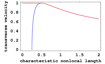
Figure 5: The area under the red line is the parameter space for gray soliton with exponential decaying nonlocal response when $\eta=1$. The left area of the blue line corresponds to gray solitons with exponentially decaying tails; the right area corresponds to gray solitons with exponentially decaying oscillatory tails.

Now we consider the nonlocal case with a Gaussian nonlocal response $R(x)={{1}\over{w\sqrt{\pi}}}\exp(-{{x^{2}}\over{w^{2}}})$. Here we only discuss the exponentially decaying oscillatory tails. However the exponentially decaying tails can be discussed in a similar way. For the exponentially decaying oscillatory tails

$$\chi(x)=\exp(-\lambda x)\cos(\kappa x),$$ (35)

we have

$$f(x) =\int_{-\infty}^{+\infty}{{1}\over{w\sqrt{\pi}}}\exp\left[-{{(x-\xi)^{2}}\over{w^{2}}}\right]\chi(\xi)d\xi$$ (36)

$$=A\chi(x)+B\chi^{\prime}(x),$$

where

$$A=e^{{w^{2}(\lambda^{2}-\kappa^{2})}\over{4}}\left(\cos{{w^{2}\lambda\kappa}\over{2}}-{{\lambda}\over{\kappa}}\sin{{w^{2}\lambda\kappa}\over{2}}\right),$$ (37)

$$B=-{{1}\over{\kappa}}e^{{w^{2}(\lambda^{2}-\kappa^{2})}\over{4}}\sin{{w^{2}\lambda\kappa}\over{2}}.$$ (38)

So Eq. (21) turns into

$$-{{1}\over{2}}\chi^{\prime\prime}+2\eta^{2}B\chi^{\prime}+(2\eta^{2}A-2\mu^{2})\chi=0.$$ (39)

The eigenvalue problem of the above equation provides two coupled equations for $\lambda$ and $\kappa$

$$\lambda=-2\eta^{2}B,$$ (40a)

$$\kappa=\sqrt{-2(2\eta^{2}A-2\mu^{2})-4\eta^{4}B^{2}}$$ (40b)

For example, when $w=5,\eta=1,\mu=0.4$, from (40) we get $\lambda=0.0733,\kappa=0.713$ which are used by the fitting function in Fig. (4).

In a similar way of deducing the parameter space in the exponentially decaying nonlocal case, we also get the parameter space in the Gaussian nonlocal case. When $w<1/\eta$, the maximal transverse velocity is a constant equal to $\eta$; when $w>1/\eta$, the maximal velocity is equal to $\sqrt{{1+\ln(\eta^{2}w^{2})}\over{w^{2}}}$. On the other hand when $w>1/\eta$, the gray soliton always has exponentially decaying oscillatory tail; When $w\leq 1/\sqrt{\rm{e}}\eta$, the gray soliton always has exponentially decaying tail; when $1/\sqrt{\rm{e}}\eta<w<1/\eta$, the gray soliton can have exponentially decaying tail for $\eta\geq\mu>\sqrt{{1+\ln(\eta^{2}w^{2})}\over{w^{2}}}$ or exponentially decaying oscillatory tail for $\mu<\sqrt{{1+\ln(\eta^{2}w^{2})}\over{w^{2}}}$. These results are shown in Fig. (6).

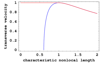
Figure 6: The area under the red line is the parameter space for gray soliton with Gaussian nonlocal response when $\eta=1$. The left area of the blue line corresponds to gray solitons with exponentially decaying tails; the right area corresponds to gray solitons with exponentially decaying oscillatory tails.

III Numerical method to compute nonlocal black soliton solutions

In the case $\mu=0$, Eq. (II) reduces to

$$\eta^{2}\psi+{{\psi^{\prime\prime}}\over{2}}-\psi\int R(x-\xi)\psi^{2}(\xi)d\xi=0.$$ (41)

We consider the nonlocal black soliton solutions with properties

$$\psi(-x)=-\psi(x)~{}~{}~{}~{}\psi(x)\xrightarrow{x\rightarrow\pm\infty}\pm\eta~{}~{}~{}~{}\psi(0)=0$$ (42)

Let

$$\chi(x)={{d\psi(x)}\over{dx}}~{}~{}~{}\rm{i.e.}~{}~{}~{}\psi(x)=\int_{0}^{x}\chi(t)dt$$ (43)

So $\chi(-x)=\chi(x)$ and $\chi(x)\xrightarrow{x\rightarrow\pm\infty}0$. Acting ${{d}\over{dx}}$ on Eq. (41), we obtain

$$\eta^{2}\chi+{{1}\over{2}}\chi^{\prime\prime}-\chi\int R(x-\xi)\psi^{2}(\xi)d\xi$$

$$-2\psi\int R(x-\xi)\psi(\xi)\chi(\xi)d\xi=0$$ (44)

Let

$$\chi(x)=\lambda\theta(x),$$ (45)

and substitute it into Eq. (III), we have

$$\eta^{2}\theta+{{1}\over{2}}\theta^{\prime\prime}-\lambda^{2}\theta\int R(x-\xi)\psi_{1}^{2}(\xi)d\xi$$

$$-2\lambda^{2}\psi_{1}\int R(x-\xi)\psi_{1}(\xi)\theta(\xi)d\xi=0,$$ (46)

Where $\psi_{1}(x)\equiv\int_{0}^{x}\theta(t)dt$. Performing DFT on Eq. (III), we have

$$\eta^{2}\widetilde{\theta}_{j}-{{\Omega_{j}}\over{2}}\widetilde{\theta}_{j}-\lambda^{2}\mathscr{F}\left[\theta\int R(x-\xi)\psi_{1}^{2}(\xi)d\xi\right]_{j}$$

$$-\lambda^{2}\mathscr{F}\left[2\psi_{1}\int R(x-\xi)\psi_{1}(\xi)\theta(\xi)d\xi\right]_{j}=0.$$ (47)

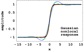
Figure 7: Amplitudes of nonlocal black soliton solutions with Gaussian nonlocal response. The parameters used are $\eta=1$ and black line $w=0$, red line $w=1$, green line $w=3$ and blue line $w=5$.

Projecting Eq. (III) onto $\widetilde{\theta}$, we obtain an equation for $\lambda$

$$~{}~{}\mathscr{A}_{\theta}(\lambda)$$

$$\equiv\sum_{j=1}^{n}\widetilde{\theta}^{*}_{j}\bigg{\{}\eta^{2}\widetilde{\theta}_{j}-\lambda^{2}\mathscr{F}\left[\theta\int R(x-\xi)\psi_{1}^{2}(\xi)d\xi\right]_{j}$$

$$-{{\Omega_{j}}\over{2}}\widetilde{\theta}_{j}-\lambda^{2}\mathscr{F}\left[2\psi_{1}\int R(x-\xi)\psi_{1}(\xi)\theta(\xi)d\xi\right]_{j}\bigg{\}}=0$$

On the other hand, from Eq. (III) we have

$$\widetilde{\theta}_{j} ={{r\widetilde{\theta}_{j}+\eta^{2}\widetilde{\theta}_{j}-\lambda^{2}\mathscr{F}\left[\theta\int R(x-\xi)\psi_{1}^{2}(\xi)d\xi\right]_{j}}\over{r+{{\Omega_{j}}\over{2}}}}$$ (49)

$$~{}~{}-{{\lambda^{2}\mathscr{F}\left[2\psi_{1}\int R(x-\xi)\psi_{1}(\xi)\theta(\xi)d\xi\right]_{j}}\over{r+{{\Omega_{j}}\over{2}}}}$$

$$\equiv\mathscr{D}_{\lambda}[\theta]_{j}$$

The iteration scheme is $\mathscr{A}_{\theta_{m}}(\lambda_{m})=0,\widetilde{\theta}_{m+1}=\mathscr{D}_{\lambda_{m}}[\theta_{m}]$. Some black nonlocal soliton solutions with Gaussian nonlocal response are shown in Fig. (7).

IV conclusion

One numerical method to compute black and gray soliton solutions with Kerr-type nonlocal nonlinearity is developed. As two examples of nonlocal cases, the gray soliton with exponentially decaying nonlocal response or with Gaussian nonlocal response are discussed. The analytical form of the tails of nonlocal gray soliton is presented. It is indicated that nonlocal gray solitons can have exponentially decaying tails or have exponentially decaying oscillatory tails. The analytical relationship for the maximal transverse velocity of nonlocal gray soliton to the characteristic nonlocal length is presented. It is indicated when the characteristic nonlocal length is less than some critical value, such maximal transverse velocity is a constant and equal to that of local gray soliton, otherwise such maximal velocity will decrease with the increasing of the characteristic nonlocal length.

- (1) S. K. Turitsyn, Teor. Mat. Fiz. , 226, (1985).
- (2) O. Bang, W. Krolikowski, J. Wyller and J. J. Rasmussen, Phys. Rev. E , 046619 (2002).
- (3) S. Skupin, O. Bang, D. Edmundson, and W. Krolikowski, Phys. Rev. E, , 066603, (2006)
- (4) Alexander I. Yakimenko, Yuri A. Zaliznyak, and Yuri Kivshar, Phys. Rev. E, , 065603, (2005).
- (5) C. Conti, M. Peccianti, G. Assanto, Phys. Rev. Lett. , 073901, (2003).
- (6) C. Conti, M. Peccianti, G. Assanto, Phys. Rev. Lett. , 113902, (2004).
- (7) W. Hu, T. Zhang, Q. Guo, L. Xuan, S. Lan, Appl. Phys. Lett. , 071111, (2006).
- (8) C. Rotschild, O. Cohen, O. Manela, M. Segev and T. Carmon, Phys. Rev. Lett. , 213904 (2005).
- (9) Q. Guo, B. Luo, F. Yi, S. Chi, Y. Xie, Phys. Rev. E, , 016602, (2004).
- (10) S. Ouyang, Q. Guo, W. Hu, Phys. Rev. E, , 036622, (2006).
- (11) S. Ouyang and Q. Guo, Phys. Rev. A, , 053833, (2007).
- (12) A. W. Snyder and D. J. Mitchell, Science , 1538 (1997).
- (13) Weiping Zhong, and Lin Yi, Phys. Rev. A, , 061801, (2007).
- (14) Daniel Buccoliero, Anton S. Desyatnikov, Wieslaw Krolikowski, and Yuri S. Kivshar, Phys. Rev. Lett. , 053901, (2007).
- (15) Dongmei Deng and Qi Guo, Opt. Lett, , 3206, (2007).
- (16) Per Dalgaard Rasmussen, Ole Bang, Wieslaw Krolikowski, Phys. Rev. E, , 066611, (2005).
- (17) Shigen Ouyang, Wei Hu, and Qi Guo, Phys. Rev. A, , 053832, (2007).
- (18) Wei Hu, Shigen Ouyang, Pingbao Yang, Qi Guo,and Sheng Lan, Phys. Rev. A, , 033842, (2008).
- (19) Wieslaw Krolikowski, Ole Bang, Phys. Rev. E, , 016610, (2000).
- (20) Alexander Dreischuh, Dragomir N. Neshev, Dan E. Petersen, Ole Bang, and Wieslaw Krolikowski, Phys. Rev. Lett. , 043901, (2006).
- (21) Nikola I. Nikolov, Dragomir Neshev and Wieslaw Krolikowski, Ole Bang, Jens Juul Rasmussen, Peter L. Christiansen, Opt. Lett, , 286, (2004).
- (22) Mark J. Ablowitz, Ziad H. Musslimani, Opt. Lett, , 2140, (2005).
- (23) G.P. Agrawal, Nonlinear Fiber Optics, New York: Academeic, 1995
- (24) Yaroslav V. Kartashov and Lluis Torner, Opt. Lett, , 946, (2007)