Finite-size scaling of string order parameters characterizing the Haldane phase

Abstract

We have developed a numerical procedure to clarify the critical behavior near a quantum phase transition by analyzing a multi-point correlation function characterizing the ground state. This work presents a successful application of this procedure to the string order parameter of the $S=1$ $XXZ$ chain with uniaxial single-ion anisotropy. The finite-size string correlation function is estimated by the density matrix renormalization group method. We focus on the gradient of the inversed-system-size dependence of the correlation function on a logarithmic plot. This quantity shows that the finite-size scaling sensitively changes at the critical point. The behavior of the gradient with increasing system size is divergent, stable at a finite value, or rapidly decreases to zero when the system is in the disordered phase, at the critical point, or in the ordered phase, respectively. The analysis of the finite-size string correlation functions allows precise determination of the boundary of the Haldane phase and estimation of the critical exponent of the correlation length. Our estimates of the transition point and the critical exponents, which are determined only by the ground-state quantities, are consistent with results obtained from the analysis of the energy-level structure. Our analysis requires only the correlation functions of several finite sizes under the same condition as a candidate for the long-range order. The quantity is treated in the same manner irrespective of the kind of elements which destroy the order concerned. This work will assist in the development of a method to directly observe quantum phase transitions.

I Introduction

Quantum phase transitions originating from quantum fluctuations have been extensively studied as a hot issue in condensed-matter physics. Several interesting characteristics of the transitions appear in the low-energy behavior of the systems. Two types of approach can capture the phase transitions and critical phenomena precisely when the transition is continuous. One is analyzing the energy-level structure. The other involves considering the ground-state behavior.

In the former approach, a standard method is to analyze the structure of the energy levels of finite-size systems based on the finite-size scaling (FSS) assumption. For example, the scaled energy gap Barber:FSS is often used to estimate the boundary of the gapped phase as the transition point. This is called phenomenological renormalization group (PRG) analysis. However, it is difficult to estimate the transition point when a logarithmic correction appears in the dependence of the energy difference. A typical example is the Berezinskii–Kosterlitz–Thouless (BKT) Transition Kosterlitz:JPC7 . To resolve this difficulty, the level-spectroscopy method has been developed Nomura:JPA28 and precise determinations of phase transitions have been successfully made for various transitions in many models. Unfortunately, this analysis is complicated in that appropriate adjustments of the procedure are required according to the type of phase transition, which must also be known in advance.

In the latter approach, on the other hand, quantities that characterize the ground state are carefully observed. One of these quantities is the multi-point correlation function. The long-range behavior of correlation functions shows whether the system exhibits long-range order. If a correlation function survives to be nonzero in the long-range limit, it is an appropriate order parameter. However, it is not easy to capture a phase transition using this strategy because reliable and precise data on correlation functions are necessary for large systems. The system sizes that are treated in numerical-diagonalization calculations are insufficient. For this reason, the latter approach has been employed in only a few studies. Therefore, no systematic procedure for analyzing ground-state quantities to capture quantum phase transitions has been established to date.

In this paper, we develop a procedure to determine the transition point and critical exponents by analyzing correlation functions based only on the scaling assumption. A feature of this approach is that only the common quantities under the same condition are treated irrespective of the type of phase transition. We call the procedure ground-state phenomenological renormalization group (GSPRG) analysis. To confirm its validity and usefulness in detecting phase transitions, we apply it to a nontrivial ground state in the AF $S=1$ $XXZ$ chain with uniaxial single-ion anisotropy by the density matrix renormalization group (DMRG) method White:PRL69 ; White:PRB48 .

In the isotropic case of this system, there exists a nonzero energy gap between the unique ground state and the first excited state, called the Haldane gapHaldane:PL93A ; Haldane:PRL50 . It is known that when anisotropy is introduced, of the single-ion type or of the $XXZ$-type exchange interaction, the Haldane gap decreases and finally closes. The region where the nonzero Haldane gap exists is called the Haldane phase. The phase diagram of the AF $S=1$ chain with anisotropy of the two types, including the Haldane phase, has been extensively studied by analyzing the energy-level structure, assisted by the level-spectroscopy method Alcaraz:PRB46 ; Hida:PRB67 ; Boschi:EPJB35 ; Boschi:EPJB41 .

It is well known that in many AF spin systems, the standard spin–spin correlation function gives so-called N$\acute{\textrm{e}}$el order. In the ground state in the Haldane phase, however, the spin–spin correlation function decays exponentially with a finite correlation length and the N$\acute{\textrm{e}}$el order no longer exists. In this sense, the Haldane phase is a disordered phase. However, the string order parameter is known to characterize the ground state in the Haldane phase, in which the longitudinal and transverse string order parameters are nonzero Nijs:PRB40 ; Kennedy:PRB45 . From the viewpoint of the string order, it is possible to treat the Haldane phase as an ordered phase and capture the phase transition at the boundary. This approach has been applied to numerical-diagonalization data of the Haldane phase in $S=1$ systemsAlcaraz:PRB46 ; Totsuka:JPCM7 ; Tonegawa:JPSJ65 . Unfortunately, only very small system sizes were available and hence it was quite difficult to capture precisely the critical behavior of the string order near the transition point.

In this situation, we can obtain numerical data of the string order of this model for much larger system sizes by using DMRG for GSPRG analysis. Consequently, it is possible to examine the phase transition at the boundary of the Haldane phase from the viewpoint of the string order. We compare our results with those from the analysis of the energy-level structure. This comparison provides a systematic and consistent understanding of the phase transition.

This paper is organized as follows. The model Hamiltonian and order parameters are defined in section II. The analysis procedure which we have developed is introduced in section III. The numerical results and discussions are given in section IV. Section V consists of a summary of this work and some remarks.

II Model Hamiltonian and order parameters

We consider the following Hamiltonian:

$$\mathcal{H}\!=\!\!\sum^{N-1}_{i=1}\!\left[J\!\left(S^{x}_{i}S^{x}_{i+1}\!+\!S^{y}_{i}S^{y}_{i+1}\right)\!+\!J_{z}S^{z}_{i}S^{z}_{i+1}\right]\!\!+\!D\!\sum^{N}_{i=1}\!{S^{z}_{i}}^{2},$$ (1)

where $N$ is the system size, $S^{\alpha}_{i}(\alpha=x,y,z)$ are spin-1 operators, $J$ and $J_{z}$ represent the $XXZ$-type anisotropic exchange interaction, and the parameter $D$ represents uniaxial single-ion anisotropy. In this paper, energies are measured in units of $J$ and hence we take $J=1$ hereafter. The boundary condition of the system is open. An antiferromagnetic chain is usually characterized by the N$\acute{\textrm{e}}$el order parameter defined as

$$O^{\alpha}_{\textrm{N}\acute{\textrm{e}}\textrm{el}}=\lim_{|i-j|\rightarrow\infty}O^{\alpha}_{\textrm{N}\acute{\textrm{e}}\textrm{el}}(i,j),$$ (2)

where $O^{\alpha}_{\textrm{N}\acute{\textrm{e}}\textrm{el}}(i,j)$ is the N$\acute{\textrm{e}}$el correlation function given by

$$O^{\alpha}_{\textrm{N}\acute{\textrm{e}}\textrm{el}}(i,j)=(-1)^{i-j}\langle S^{\alpha}_{i}S^{\alpha}_{j}\rangle.$$ (3)

Here $\langle\hat{B}\rangle$ represents the ground-state expectation value of an arbitrary operator $\hat{B}$. In the Haldane phase, the N$\acute{\textrm{e}}$el order parameter vanishes. However, the string order introduced by den Nijs and Rommelse Nijs:PRB40 appears instead. The string order parameter is given by

$$O^{\alpha}_{\textrm{str}}=\lim_{|i-j|\rightarrow\infty}O^{\alpha}_{\textrm{str}}(i,j),$$ (4)

where the string correlation function $O^{\alpha}_{\textrm{str}}(i,j)$ is given by

$$O^{\alpha}_{\textrm{str}}(i,j)=-\left\langle S^{\alpha}_{i}\exp\left[i\pi\sum^{j-i}_{k=i+1}S^{\alpha}_{k}\right]S^{\alpha}_{j}\right\rangle.$$ (5)

Kennedy and Tasaki Kennedy:PRB45 extensively studied the string order and applied a nonlocal unitary transformation to the Hamiltonian (1). Thereby they obtained

$$O^{\alpha}_{\textrm{str}} =O^{\alpha}_{\textrm{ferro}}(\tilde{\mathcal{H}})\>\>\>\textrm{for}\>\alpha=x\>\textrm{or}\>z,$$ (6)

where $O^{\alpha}_{\textrm{ferro}}=\lim_{|i-j|\rightarrow\infty}\left\langle S^{\alpha}_{i}S^{\alpha}_{j}\right\rangle$, and $\tilde{\mathcal{H}}$ is obtained by applying the transformation to the original Hamiltonian $\mathcal{H}$. In the transformed system, $\mathbb{Z}_{2}\times\mathbb{Z}_{2}$ symmetry emerges. Breaking of this symmetry is described by the behavior of the order parameters $O^{\alpha}_{\textrm{ferro}}(\tilde{\mathcal{H}})$. When the system is in the Haldane phase, this $\mathbb{Z}_{2}\times\mathbb{Z}_{2}$ symmetry is fully broken. When the chain is in a phase other than the Haldane phase, the full symmetry or a part of the symmetry survives Kennedy:PRB45 ; Alcaraz:PRB46 ; Hatsugai:PRB44 .

III Analysis procedure

In this section we introduce our analysis procedure. The procedure consists of three steps. The first is to calculate the longitudinal and transverse order parameters by the DMRG method based on the finite-size algorithm White:PRL69 ; White:PRB48 . Knowing the behavior of the order parameters enables us to observe the boundary of the Haldane phase briefly and to confirm that the transition at the boundary is continuous. If we apply the FSS analysis of the order parameters Tonooka:JPSJ76 , we can roughly estimate the critical point and exponents. However, there remain finite-size effects in these estimates. In order to eliminate the effects, we carry out a finite-size extrapolation derived from the FSS formula. As the second step, we introduce a finite-size quantity which we calculate from the string order parameters. This quantity reaches the critical exponent just at the phase boundary when we take the limit $N\rightarrow\infty$. By examining the behavior of this quantity, it is possible to obtain the phase boundary and the critical exponent of the order parameter at the transition point. At the third step, we estimate the critical exponent of the correlation length near the transition point by extrapolating a finite-size quantity at the above transition point. The present procedure gives consistent and precise estimates for the critical point and exponents.

III.1 Calculation of order parameters

To calculate the order parameters, we use the finite DMRG algorithm with the acceleration algorithm introduced by White White:PRL69 ; White:PRB48 ; White:PRL77 . A correlation function, such as Eq. (3) or Eq. (5), is calculated as follows. First, we obtain a variational wave function of the ground state represented by the matrix product state (MPS):

$$\left|\Phi\right\rangle=\sum_{\{s\}}\sum_{\{\alpha\}}\left(U_{s_{1},\alpha_{2}}^{[2],s_{2}}U_{\alpha_{2},\alpha_{3}}^{[3],s_{3}}\cdots U_{\alpha_{N/2-2},\alpha_{N/2-1}}^{[N/2-1],s_{N/2-1}}\right.\hskip 28.45274pt$$

$$A_{\alpha_{N/2-1},\alpha_{N/2+2}}^{s_{N/2},s_{N/2+1}}V_{\alpha_{N/2+2},\alpha_{N/2+3}}^{[N/2+2],s_{N/2+2}}\cdots\hskip 25.60747pt$$

$$\left.V_{\alpha_{N-2},\alpha_{N-1}}^{[N-2],s_{N-2}}V_{\alpha_{N-1},s_{N}}^{[N-1],s_{N-1}}\right)\left|s_{1}s_{2}\cdots s_{N}\right\rangle,$$

$$(\{s\}=s_{1},s_{2},\cdots,s_{N},\hskip 5.69054pt\{\alpha\}=\alpha_{2},\alpha_{3},\cdots,\alpha_{N-1}),$$ (7)

where $U$ and $V$ are matrices satisfying

$$U^{[i]\dagger}U^{[i]} =\mathbf{1}, (i=2,\cdots,N/2-1),$$ (8a)

$$V^{[j]}V^{[j]\dagger} =\mathbf{1}, (j=N/2+2,\cdots,N-1),$$ (8b)

respectively, and $A$ is the ground state of the renormalized Hamiltonian which is obtained by applying the density matrix renormalization transformation to the Hamiltonian (1). A truncation error $\epsilon$ due to the cut off $m_{\rm F}$ is estimated by $1-\textrm{Tr}\left(A^{*}A\right)$, where $m_{\rm F}$ is the number of states preserved in the DMRG iterations White:PRL69 . Using this wave function, we estimate the expectation value $O^{\alpha}_{\textrm{str}}(i,j)$ as follows:

$$O^{\alpha}_{\textrm{str}}(i,j)=-\left\langle\Phi\right|S^{\alpha}_{i}\tilde{S}^{\alpha}_{i+1}\cdots\tilde{S}^{\alpha}_{j-1}S^{\alpha}_{j}\left|\Phi\right\rangle$$

$$=-\textrm{Tr}\left(E^{[2]}_{\mathbf{1},\mathbf{1}}E^{[3]}_{\mathbf{1}}\cdots E^{[i-1]}_{\mathbf{1}}E^{[i]}_{S^{\alpha}_{i}}E^{[i+1]}_{\tilde{S}^{\alpha}_{i+1}}\right.\cdots\hskip 22.76219pt$$

$$E^{[N/2-1]}_{\tilde{S}^{\alpha}_{N/2-1}}E^{[A]}_{\tilde{S}^{\alpha}_{N/2},\tilde{S}^{\alpha}_{N/2+1}}E^{[N/2+2]}_{\tilde{S}^{\alpha}_{N/2+2}}\cdots\hskip 14.22636pt$$

$$\left.E^{[j-1]}_{\tilde{S}^{\alpha}_{j-1}}E^{[j]}_{S^{\alpha}_{j}}E^{[j+1]}_{\mathbf{1}}\cdots E^{[N-2]}_{\mathbf{1}}E^{[N-1]}_{\mathbf{1},\mathbf{1}}\right).$$ (9)

Here, $\mathbf{1}$ is the identity matrix in spin-1 space and $\tilde{S}^{\alpha}$ is defined as $\tilde{S}^{\alpha}=\exp(i\pi S^{\alpha})$. Each $E$ is a matrix for an arbitrary local operator $O$ defined by

$$E^{[2]}_{O,O}\! = \sum_{s_{1},s_{1}^{\prime},s_{2},s_{2}^{\prime}}\left\langle s_{1}\right|O\left|s_{1}^{\prime}\right\rangle\left\langle s_{2}\right|O\left|s_{2}^{\prime}\right\rangle\hskip 65.44133pt$$

$$U_{s_{1}}^{[2],s_{2}}\otimes\left(U_{s_{1}^{\prime}}^{[2],s_{2}^{\prime}}\right)^{*},\hskip 11.38109pt$$ (10a)

$$E^{[i]}_{O} = \sum_{s_{i},s_{i}^{\prime}}\left\langle s_{i}\right|O\left|s_{i}^{\prime}\right\rangle U^{[i],s_{i}}\otimes\left(U^{[i],s_{i}^{\prime}}\right)^{*},\hskip 39.83385pt$$

$$(3\leq i\leq N/2-1),\hskip 14.22636pt$$ (10b)

$$E^{[A]}_{O,O} = \sum_{s_{k},s_{k}^{\prime},s_{k+1},s_{k+1}^{\prime}}\!\!\!\!\!\!\left\langle s_{k}\right|O\left|s_{k}^{\prime}\right\rangle\left\langle s_{k+1}\right|O\left|s_{k+1}^{\prime}\right\rangle\hskip 36.98857pt$$

$$A^{s_{k},s_{k+1}}\otimes\left(A^{s_{k}^{\prime},s_{k+1}^{\prime}}\right)^{*},\hskip 14.22636pt$$

$$(k=N/2),\hskip 14.22636pt$$ (10c)

$$E^{[j]}_{O} = \sum_{s_{j},s_{j}^{\prime}}\left\langle s_{j}\right|O\left|s_{j}^{\prime}\right\rangle V^{[j],s_{j}}\otimes\left(V^{[j],s_{j}^{\prime}}\right)^{*},\hskip 28.45274pt$$

$$(N/2+2\leq j\leq N-2),\hskip 14.22636pt$$ (10d)

$$E^{[N-1]}_{O,O} = \sum_{s_{N-1},s_{N-1}^{\prime},s_{N},s_{N}^{\prime}}\left\langle s_{N-1}\right|O\left|s_{N-1}^{\prime}\right\rangle\left\langle s_{N}\right|O\left|s_{N}^{\prime}\right\rangle\hskip 31.29802pt$$

$$V_{s_{N}}^{[N-1],s_{N-1}}\otimes\left(V_{s_{N}^{\prime}}^{[N-1],s_{N-1}^{\prime}}\right)^{*}.\hskip 14.22636pt$$ (10e)

When calculating a two-point correlation function such as Eq. (3), we replace all the operators $\tilde{S}^{\alpha}$ with $\mathbf{1}$. We also choose an appropriate correlation function as the longest-ranged component from among $O^{\alpha}_{\textrm{str}}(i,j)$ or $O^{\alpha}_{\textrm{N}\acute{\textrm{e}}\textrm{el}}(i,j)$ for a fixed $N$ under the open boundary condition. Three desirable conditions should be met, as follows.

1. The measurement points $i$ and $j$ are as far as possible from the edges.

2. The correlation distance of $|j-i|$ is as long as possible.

3. The distance $|j-i|$ should increase in proportion to the system size $N$.

In order to satisfy the above conditions, we take $i=N/3+1$ and $j=2N/3$. Thus, we consider the order parameter

$$O^{\alpha}(N,D,J_{z}) =O^{\alpha}(N/3+1,2N/3,D,J_{z}),$$ (11)

where $\alpha=x,z$, $O^{\alpha}$ represents $O^{\alpha}_{\textrm{N}\acute{\textrm{e}}\textrm{el}}$ or $O^{\alpha}_{\textrm{str}}$. Note here that $N/6$ should be an integer. We emphasize again that Eq. (11) is useful in the case of the open boundary condition comment_PBC .

The error of the order parameters is estimated as follows.

1. $\left\langle O^{\alpha}\right\rangle_{m_{1}}$ is calculated in the case of $m_{1}=0.95\times m_{\textrm{F}}$.

2. $\left\langle O\right\rangle_{m=m_{2}}$ and the truncation error $\epsilon$ are calculated in the case of $m_{2}=m_{\textrm{F}}$.

3. The error estimation of the order parameters $\left\langle O^{\alpha}\right\rangle^{\textrm{error}}_{m_{\textrm{F}}}$ is defined by the following formula:

   $$\left\langle O^{\alpha}\right\rangle^{\textrm{error}}_{m_{\textrm{F}}}=\max\left[\left|\left\langle O^{\alpha}\right\rangle_{m_{2}}-\left\langle O^{\alpha}\right\rangle_{m_{1}}\right|,\left|\epsilon\left\langle O^{\alpha}\right\rangle_{m_{2}}\right|\right].$$ (12)

In this paper, all numerical data have a truncation error $\epsilon<10^{-7}$.

III.2 Finite-size scaling analysis

In the general theory of phase transitions, the treatment of physical quantities depends on whether the transition is continuous or discontinuous. If the transition is continuous, the critical behavior of bulk quantities is extracted through the FSS analysis of finite-size quantities Barber:FSS . As we observe later, the DMRG data of correlation functions of the finite-size systems are continuous near the boundary of the Haldane phase. The exact-diagonalization data of the string order parameters are also continuous. Thus, it is possible to perform FSS analysis of our DMRG data of the string order parameter.

The present model includes two control parameters, $D$ and $J_{z}$. When $J_{z}$ is fixed and $D$ is varied, we carry out the FSS analysis based on the following equation:

$$O^{\alpha}_{\textrm{str}}(N,D,J_{z}^{\textrm{fix}})=N^{-\eta_{\alpha}}\Psi((D_{\textrm{c}}-D)N^{1/\nu_{\alpha}}),$$ (13)

where $\alpha=x$ or $z$, $J_{z}^{\textrm{fix}}$ is the fixed $J_{z}$, and $D_{\textrm{c}}$ is the critical point. The same equation concerning the string-type order parameter was used in Ref. Tonooka:JPSJ76 . The exponents $\eta_{\alpha}$ and $\nu_{\alpha}$ are defined as

$$\xi(N=\infty,D,J_{z}^{\textrm{fix}}) \sim(D_{\textrm{c}}-D)^{-\nu},$$ (14a)

$$O^{\alpha}_{\textrm{str}}(N,D_{\textrm{c}},J_{z}^{\textrm{fix}}) \sim N^{-\eta_{\alpha}},$$ (14b)

where $\xi(N,D,J_{z})$ represents the correlation length. When $D$ is fixed and $J_{z}$ is varied, on the other hand, the FSS formula is given by

$$O^{\alpha}_{\textrm{str}}(N,D^{\textrm{fix}},J_{z})=N^{-\eta_{\alpha}}\Psi((J^{\textrm{c}}_{z}-J_{z})N^{1/\nu_{\alpha}}),$$ (15)

where the critical exponents $\eta_{\alpha}$ and $\nu_{\alpha}$ are given by

$$\xi(N=\infty,D^{\textrm{fix}},J_{z}) \sim(J^{\textrm{c}}_{z}-J)^{-\nu},$$ (16a)

$$O^{\alpha}_{\textrm{str}}(N,D^{\textrm{fix}},J^{\textrm{c}}_{z}) \sim N^{-\eta_{\alpha}}.$$ (16b)

Note that as the BKT transition point is approached, only Eq. (14b) or Eq. (16b) is realized. In this case, the correlation length grows exponentially Kosterlitz:JPC7 ; the dependence is different from Eq. (14a) or Eq. (16a), having a finite exponent.

Successfully obtaining a universal function $\Psi$ irrespective of the system size $N$ in the critical region near the critical point, allows us to determine the critical point and critical exponents. However, the FSS analysis still has a problem in that the width of the critical region is unknown. Since the width depends on the values of the control parameters, it is difficult to determine or estimate an appropriate width. To avoid this difficulty, we perform the extrapolation explained below.

III.3 Ground-state phenomenological-renormalization-group analysis

In this paper, we perform a procedure to obtain the transition point and the critical exponents consistently considering the ground-state quantities. We call this procedure the ground-state phenomenological-renormalization-group (GSPRG) analysis. The first step of the procedure is to examine a finite-size quantity defined as

$$\eta_{\alpha}(\tilde{N},D,J_{z})\!=\!\frac{\log\left[O^{\alpha}_{\textrm{str}}(N_{2},D,J_{z})/O^{\alpha}_{\textrm{str}}(N_{1},D,J_{z})\right]}{\log[N_{1}/N_{2}]},$$ (17)

where $\tilde{N}=(N_{1}+N_{2})/2$, $N_{2}=\Delta N+N_{1}$, and $\Delta N=6$. Here, we examine the direction $\alpha$ such that $O^{\alpha}_{\textrm{str}}$ shows critical behavior. The quantity indicates the gradient of the curve of the dependence of $O^{\alpha}_{\textrm{str}}$ on $1/N$ in a plot with both the axes on the logarithmic scale. The gradient should be constant for large system sizes when the set of $D$ and $J_{z}$ corresponds to the boundary of the Haldane phase. The quantity $\eta_{\alpha}(\tilde{N},D,J_{z})$ converges to the critical exponent $\eta_{\alpha}$ defined by Eq. (14b) or Eq. (16b) for ($D$, $J_{z}$) on the boundary; the $\tilde{N}$ dependence of $\eta_{\alpha}(\tilde{N},D,J_{z})$ shows a stable convergence to a finite value when the system size is increased. On the other hand, when the point ($D$, $J_{z}$) is not on the boundary, $\eta_{\alpha}(\tilde{N},D,J_{z})$ shows a different behavior. For ($D$, $J_{z}$) inside the Haldane phase, $O^{\alpha}_{\textrm{str}}$ tends towards a nonzero value as $N$ is increased. Thus the gradient $\eta_{\alpha}(\tilde{N},D,J_{z})$ rapidly decreases. For ($D$, $J_{z}$) outside the Haldane phase, $O^{\alpha}_{\textrm{str}}$ decays rapidly with increasing $N$. This decay is more rapid than that for Eq. (14b) or Eq. (16b). In this case, the gradient $\eta_{\alpha}(\tilde{N},D,J_{z})$ rapidly increases. Therefore, we can find the critical point from the difference in the $\tilde{N}$-dependence of $\eta_{\alpha}(\tilde{N},D,J_{z})$. The difference is expected to be more apparent when $\tilde{N}$ increases sufficiently to diminish the edge effect. In order to estimate the critical point, we have investigated the behavior of $\eta_{\alpha}(\tilde{N},D,J_{z})$ for $N=6,12,\cdots,90,96$ and found the characteristic behavior of $\eta_{\alpha}(\tilde{N},D,J_{z})$ in the region of large $\tilde{N}$. The numerical procedure to determine the critical point by observing the behavior of $\eta_{\alpha}(\tilde{N},D,J_{z})$ is as follows.

• When the differentiation of the finite-size quantity $\eta_{\alpha}(\tilde{N},D,J_{z})$ satisfies the following conditions for a large system size,

  $$\eta^{(1)}_{\alpha}(\tilde{N},D,J_{z})>0\wedge\eta^{(2)}_{\alpha}(\tilde{N},D,J_{z})>0,$$ (18a)

  $${\rm or}\hskip 85.35826pt$$

  $$\eta^{(1)}_{\alpha}(\tilde{N},D,J_{z})<0\wedge\eta^{(2)}_{\alpha}(\tilde{N},D,J_{z})<0,$$ (18b)

  we can consider that the system with $(D,J_{z})$ is at a critical point. Here $\eta^{(n)}_{\alpha}(\tilde{N},D,J_{z})(n=1,2)$ is the numerical differentiation given by

  $$\eta^{(n)}_{\alpha}(\tilde{N},D,J_{z})=\left(\frac{\partial}{\partial(1/\tilde{N})}\right)^{n}\eta_{\alpha}(\tilde{N},D,J_{z}).$$ (19)

  The differentiation is approximated by the difference because $\tilde{N}$ is integer or half integer.

• If the differentiation reveals

  $$\eta^{(1)}_{\alpha}(\tilde{N},D,J_{z})>0\wedge\eta^{(2)}_{\alpha}(\tilde{N},D,J_{z})<0,$$ (20)

  we can consider that $\eta_{\alpha}(\tilde{N},D,J_{z})$ will decrease rapidly with increasing system size. In this case, the system with $(D,J_{z})$ is in the ordered phase with respect to the string order.

• If the differentiation satisfies

  $$\eta^{(1)}_{\alpha}(\tilde{N},D,J_{z})<0\wedge\eta^{(2)}_{\alpha}(\tilde{N},D,J_{z})>0,$$ (21)

  we can consider that $\eta_{\alpha}(\tilde{N},D,J_{z})$ will increase rapidly with increasing system size. In this case, the system with $(D,J_{z})$ is in the disordered phase with respect to the string order.

We summarize the difference in the behavior of $\eta_{\alpha}(\tilde{N},D,J_{z})$ in Table 1. Now, the boundary for a finite-size system between the critical region and the string-ordered phase is given by $N^{\prime}$ defined in

$$\eta^{(1)}_{\alpha}(N^{\prime},D,J_{z})>0\wedge\eta^{(2)}_{\alpha}(N^{\prime},D,J_{z})=0,$$ (22a)

$${\rm or}\hskip 85.35826pt$$

$$\eta^{(1)}_{\alpha}(N^{\prime},D,J_{z})=0\wedge\eta^{(2)}_{\alpha}(N^{\prime},D,J_{z})<0,$$ (22b)

to find a boundary between Eq. (18a, 18b) and Eq. (20). We obtain $N^{\prime}$ as a real positive number because $\eta^{(i)}_{\alpha}(N^{\prime},D,J_{z})$ is an interpolated value of $\eta^{(i)}_{\alpha}(\tilde{N},D,J_{z})$ for $i=1,2$. The boundary between the critical region and the string disordered phase is, on the other hand, given by $N^{\prime}$ defined in

$$\eta^{(1)}_{\alpha}(N^{\prime},D,J_{z})=0\wedge\eta^{(2)}_{\alpha}(N^{\prime},D,J_{z})>0,$$ (23a)

$${\rm or}\hskip 85.35826pt$$

$$\eta^{(1)}_{\alpha}(N^{\prime},D,J_{z})<0\wedge\eta^{(2)}_{\alpha}(N^{\prime},D,J_{z})=0,$$ (23b)

to find a boundary between Eq. (18a, 18b) and Eq. (21). When the critical behavior appears only at a point, the width between the critical-ordered boundary and the critical-disordered boundary shrinks as $N^{\prime}$ increases. Such behavior will be presented in section IV.2. In this work, we consider the width of the critical region between the two boundaries to be an error in our analysis of the transition point if the width is very narrow. In a case of the BKT transition, the critical-disordered boundary does not appear. In this case, we must estimate the transition point carefully only from the critical-ordered boundary. Details of this treatment will be given in section IV.4.

Table 1: Behavior of $\eta_{\alpha}(\tilde{N},D,J_{z})$ in the four phases and near the three transition lines. HN, HL, HX: Haldane-N$\acute{\textrm{e}}$el, Haldane-Large-$D$, Haldane-$XY$. RD, RI, SF: rapidly decreasing finite-size exponent (17), rapidly increasing exponent, stably finite exponent, as the system size is increased.

	Haldane	HN transition line	N$\acute{\textrm{e}}$el
$\eta_{x}(\tilde{N},D,J_{z})$	RD	SF	RI
$\eta_{z}(\tilde{N},D,J_{z})$	RD	RD	RD
	Haldane	HL transition line	Large-$D$
$\eta_{\alpha}(\tilde{N},D,J_{z})$	RD	SF	RI
	Haldane	HX transition line	$XY$
$\eta_{\alpha}(\tilde{N},D,J_{z})$	RD	SF	SF

The estimation of $\eta_{\alpha}$ of the string order parameter by PRG analysis has been reported by Hida Hida:JPSJ62 based on finite-size data of the string orders by an exact diagonalization (ED) method. Since the system size is limited to being very small, however, the finite-size effect becomes significant. To avoid this difficulty as much as possible, Hida combined the critical point determined from the energy gap under the open boundary condition and the string correlation functions under the periodic boundary condition. For our purposes, we impose only the open boundary condition for our DMRG calculations and employ a definition of the string order Eq. (11) as the longest-ranged component.

In the final stage of the present analysis, we estimate the critical exponents $\nu_{\alpha}(D_{c},J^{\textrm{fix}}_{z})$ and $\nu_{\alpha}(D^{\textrm{fix}},J^{\textrm{c}}_{z})$. We first consider the case where $D$ is controlled for a fixed $J_{z}$. Within the FSS analysis based on Eq. (13), an appropriate set of $D_{\textrm{c}}$, $\eta_{\alpha}$, and $\nu_{\alpha}$ is expected to give a universal function $\Psi$ near $D=D_{c}$ independent of $N$. However, it is difficult to determine the width of the critical region, as we have mentioned. We instead focus our attention on the gradient of the universal function $\Psi$ at $D=D_{\rm c}$. We note that the $N$-independence of the gradient is a necessary condition for the existence of the universal function $\Psi$ near $D=D_{c}$. Therefore, we assume that the gradient for $N=N_{1}$ and that for $N=N_{2}$ agree with each other for the same $D_{\textrm{c}}$, $\eta_{\alpha}$, and $\nu_{\alpha}$, to give

$$\left.N_{1}^{\eta_{\alpha}-1/\nu_{\alpha}}\frac{\partial[O^{\alpha}_{\textrm{str}}(N_{1},D,J^{\textrm{fix}}_{z})]}{\partial D}\right|_{D=Dc}\hskip 28.45274pt$$

$$=\left.N_{2}^{\eta_{\alpha}-1/\nu_{\alpha}}\frac{\partial[O^{\alpha}_{\textrm{str}}(N_{2},D,J^{\textrm{fix}}_{z})]}{\partial D}\right|_{D=Dc}$$ (24)

We input $D_{\textrm{c}}$ and $\eta_{\alpha}(\tilde{N},D,J_{z})$ determined above into $D$ and $\eta$ in this equation and solve with respect to $1/\nu_{\alpha}$. Denoting the solution by $1/\nu_{\alpha}(\tilde{N},D_{c},J^{\textrm{fix}}_{z})$, we obtain

$$\frac{1}{\nu_{\alpha}(\tilde{N},D_{c},J^{\textrm{fix}}_{z})}=\eta_{\alpha}(\tilde{N},D_{\textrm{c}},J^{\textrm{fix}}_{z})\hskip 56.9055pt$$

$$+\frac{\log[(O^{\prime})^{\alpha}_{\textrm{str}}(N_{2},D_{\textrm{c}},J^{\textrm{fix}}_{z})/(O^{\prime})^{\alpha}_{\textrm{str}}(N_{1},D_{\textrm{c}},J^{\textrm{fix}}_{z})]}{\log[N_{2}/N_{1}]},$$ (25)

where $(O^{\prime})^{\alpha}_{\textrm{str}}(N,D_{\textrm{c}},J^{\textrm{fix}}_{z})$ represents

$$(O^{\prime})^{\alpha}_{\textrm{str}}(N,D_{\textrm{c}},J^{\textrm{fix}}_{z})=\left.\frac{\partial O^{\alpha}_{\textrm{str}}(N,D,J_{z}^{\textrm{fix}})}{\partial D}\right|_{D=D_{\textrm{c}}}.$$ (26)

We note that $\nu_{\alpha}(\tilde{N},D_{c},J^{\textrm{fix}}_{z})$ is a finite-size quantity and we examine the $N$-dependence of this quantity. An extrapolation to the limit $\tilde{N}\rightarrow\infty$ provides the exponent $\nu_{\alpha}(D_{\textrm{c}},J^{\textrm{fix}}_{z})$. Hereafter, we call $\eta_{\alpha}(\tilde{N},D,J_{z})$ and $\nu_{\alpha}(\tilde{N},D_{c},J^{\textrm{fix}}_{z})$ the finite-size exponents.

We next consider the case where $J_{z}$ is controlled for a fixed $D$. The same derivation as the above from Eq. (15) leads to the finite-size exponent:

$$\frac{1}{\nu_{\alpha}(\tilde{N},D^{\textrm{fix}},J^{\textrm{c}}_{z})}=\eta_{\alpha}(\tilde{N},D^{\textrm{fix}},J^{\textrm{c}}_{z})\hskip 56.9055pt$$

$$+\frac{\log[(O^{\prime})^{\alpha}_{\textrm{str}}(N_{2},D^{\textrm{fix}},J^{\textrm{c}}_{z})/(O^{\prime})^{\alpha}_{\textrm{str}}(N_{1},D^{\textrm{fix}},J^{\textrm{c}}_{z})]}{\log[N_{2}/N_{1}]},$$ (27)

where $(O^{\prime})^{\alpha}_{\textrm{str}}(N,D^{\textrm{fix}},J^{\textrm{c}}_{z})$ represents

$$(O^{\prime})^{\alpha}_{\textrm{str}}(N,D^{\textrm{fix}},J^{\textrm{c}}_{z})=\left.\frac{\partial O^{\alpha}_{\textrm{str}}(N,D^{\textrm{fix}},J_{z})}{\partial J_{z}}\right|_{J_{z}=J_{z}^{\textrm{c}}}.$$ (28)

The extrapolation of $\nu_{\alpha}(\tilde{N},D^{\textrm{fix}},J^{\textrm{c}}_{z})$ gives the exponent $\nu_{\alpha}(D^{\textrm{fix}},J^{\textrm{c}}_{z})$.

IV Results and discussions

IV.1 Behavior of order parameters

Let us first review the behavior of the four order parameters under consideration in a finite-size system and summarize some important relations between them. In a moderately large system, we can see indications of asymptotic behavior in each order parameter, although slow convergence prevents a full description. Some are characteristic for a given region of the parameter space, which is specified as one of the Haldane, N$\acute{\textrm{e}}$el, Large-D, and $XY$ phases.

We illustrate $O^{\alpha}_{\rm str}(300,D,J_{z})$ and $O^{\alpha}_{\rm N\acute{\textrm{e}}el}(300,D,J_{z})$ with $\alpha=x$ or $z$ in Fig. 1. The $D$-dependences of the order parameters on the line $J_{z}=0.5$ and their $J_{z}$-dependences on the line $D=0$ are shown in Fig. 1(a) and 1(b), respectively.

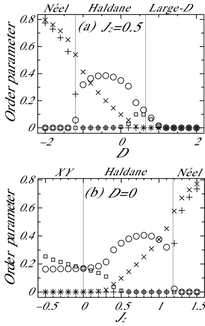
Figure 1: $(D,J_{z})$ dependence of the order parameters for the Hamiltonian (1) on (a) the $J_{z}=0.5$ line and (b) the $D=0$ line at $N=300$. $+$: $O^{z}_{\textrm{N}\acute{\textrm{e}}\textrm{el}}$, $\times$: $O^{z}_{\textrm{str}}$, $\square$: $O^{x}_{\textrm{N}\acute{\textrm{e}}{\textrm{el}}}$, $\bigcirc$: $O^{x}_{\textrm{str}}$.

We now compare the magnitudes of the four order parameters. (i) If $J_{z}>0$, $O^{\alpha}_{\textrm{str}}$ is larger than $O^{\alpha}_{\textrm{N}\acute{\textrm{e}}{\textrm{el}}}$. This is a known relation found by Kennedy and Tasaki Kennedy:CMP147 . (ii) When $D=0$ and $J_{z}=1$, we have $O^{x}_{\textrm{str}}=O^{z}_{\textrm{str}}$ due to the isotropy of the system. (iii) When $J_{z}$ is decreased and when $J_{z}$ crosses a critical point at $J_{z}=0$, $O^{x}_{\textrm{str}}$ is smaller than $O^{x}_{\textrm{N}\acute{\textrm{e}}{\textrm{el}}}$. This fact will be discussed and utilized in §IV.4. Although $O^{x}_{\textrm{N}\acute{\textrm{e}}\textrm{el}}$ appears to be nonzero around $0<D<1$ with $J_{z}=0.5$ and around $0<J_{z}<0.5$ with $D=0$, we can confirm that $O^{x}_{\textrm{N}\acute{\textrm{e}}{\textrm{el}}}$ in this region vanishes for the long-ranged limit. On the other hand, $O^{z}_{\textrm{str}}$ around $0<J_{z}<0.4$ with $D=0$ looks very small but it survives as a nonzero quantity in an infinite system, as shown in §IV.

The phase boundaries of Haldane–N$\acute{\textrm{e}}$el, Haldane–Large-$D$, and Haldane–$XY$ are denoted by dotted lines, though they are given only as indicators as we will determine the boundaries in the following subsections. We can see that some or all of the order parameters vanish at the phase boundaries. Also, the order parameters are continuous around the boundaries, which suggests that the phase transitions are continuous. Therefore, the FSS analysis and the GSPRG procedure are feasible for capturing critical phenomena in this case, except for the Berezinskii–Kosterlitz–Thouless (BKT) transition which does not satisfy the conditions of Eq. (14a) or (16a) and thus requires extra consideration. For GSPRG, however, it is possible for us to capture the transition by looking at the exponent $\eta_{\alpha}$ as discussed in §IV.4.

We next observe the behavior of the four order parameters in each phase to determine their thermodynamic limits. In Fig. 2, we illustrate the behavior of the order parameters (11) as a function of the inverse of the system size at the representative points $(D,J_{z})=(-2,0.5)$, $(2,0.5)$, $(0,0.5)$, and $(0,-0.5)$. These sets of parameters correspond to the N$\acute{\textrm{e}}$el phase, Large-$D$ phase, Haldane phase, and $XY$ phase, respectively.

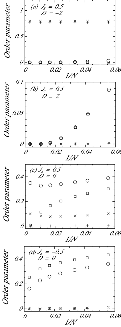
Figure 2: Order parameters for the Hamiltonian (1) as a function of the inverse of the system size. Each panel represents (a) the N$\acute{\textrm{e}}$el phase, (b) the Large-$D$ phase, (c) the Haldane phase, and (d) the $XY$ phase. $+$: $O^{z}_{\textrm{N}\acute{\textrm{e}}{\textrm{el}}}$, $\times$: $O^{z}_{\textrm{str}}$, $\square$: $O^{x}_{\textrm{N}\acute{\textrm{e}}\textrm{el}}$, $\bigcirc$: $O^{x}_{\textrm{str}}$.

We observe that in the N$\acute{\textrm{e}}$el phase, only the order parameters in the $z$ direction remain nonzero in the limit $N\rightarrow\infty$. All the four parameters vanish in the Large-$D$ phase in the thermodynamic limit. We note that in the Haldane phase, only the string order parameters in the two directions remain nonzero in the thermodynamic limit. It is difficult to judge in Fig. 2(d) whether both of the transverse order parameters in the $XY$ phase vanish or remain nonzero in the thermodynamic limit. We plot the same data on a logarithmic scale in Fig. 3.

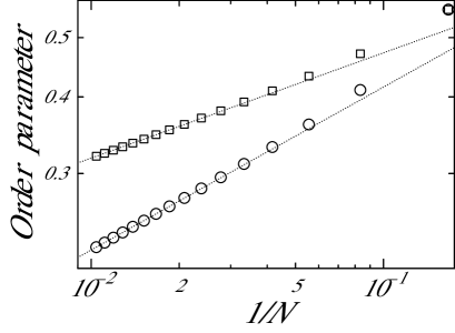
Figure 3: Order parameters for the Hamiltonian (1) in the $XY$ phase as a function of $1/N$. A fitting based on $O(N)=C_{1}N^{-\gamma}$ is carried out for $N=96,90,\cdots,72$. $\square$: $O^{x}_{\textrm{N}\acute{\textrm{e}}\textrm{el}}$, $\bigcirc$: $O^{x}_{\textrm{str}}$.

For large $N$, the data exhibits a linear behavior, which suggests that the transverse order parameters in the $XY$ phase are critical, consistent with previous reports Alcaraz:PRB46 ; Hatsugai:PRB44 . Consequently we can confirm that the order parameter $O^{\alpha}(\infty,0,-0.5)$ vanishes in the $XY$ phase. in the limit $N\rightarrow\infty$.

IV.2 Haldane–Large-$D$ transition line

In this subsection, we examine the transition from the Haldane phase to the large-$D$ phase. This transition is known to be of Gaussian type. As we observe in §IV.1, the string order parameters in the Haldane phase remain nonzero for both $\alpha=x$ and $z$ while both of the N$\acute{\textrm{e}}$el order parameters vanish along the directions $x$ and $z$. We also observe critical behavior near the transition line in both $O^{x}_{\textrm{str}}$ and $O^{z}_{\textrm{str}}$.

To begin with, we consider difficulties in the FSS analysis near the transition between the two phases. In this analysis, we have adjusted the critical point $D_{\rm c}$ and exponents $\eta_{\alpha}$ and $\nu_{\alpha}$ so that the data for $N=24$, 48, and 96 follows a universal function. The results are depicted in Fig. 4.

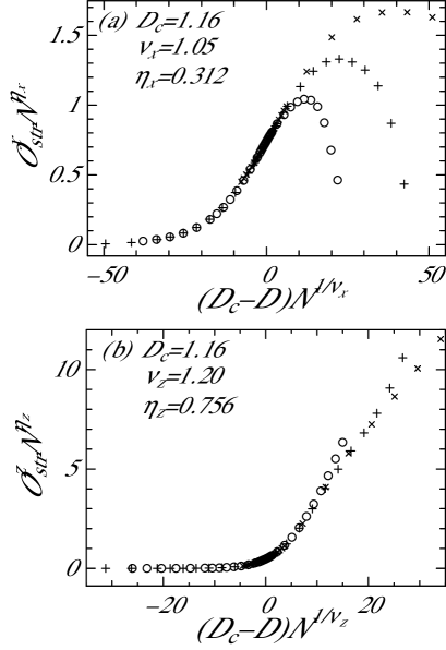
Figure 4: FSS of (a) the transverse string order and (b) the longitudinal string order on $J_{z}=1.25$ near the Haldane–Large-$D$ critical point. $\bigcirc$, $+$, and $\times$ represent $N=24,48,96$.

In Fig. 4(a), we observe a deviation from the universal function $\Psi$ at $D$, not far from $D=D_{\rm c}$. The appearance of this deviation depends on the system size and the direction $\alpha$. Thus, it is not easy to determine the critical region around $D=D_{\rm c}$ with finite-size data less than 100 sites in this case.

Despite this difficulty, we can choose input parameters $D_{\rm c}$, $\nu_{\alpha}$, and $\eta_{\alpha}$ such that a universal function $\Psi$ appears near the transition point. In Fig. 4(a), the string correlation functions in the direction $\alpha=x$ provide us with $D^{\textrm{HL}}_{\textrm{c}}(J_{z}=1.25)=1.16$ and $\nu_{x}(D=1.16,J_{z}=1.25)=1.05$. On the other hand, in Fig. 4(b), the string correlation functions in $\alpha=z$ give $D^{\textrm{HL}}_{\textrm{c}}(J_{z}=1.25)=1.16$ and $\nu_{z}(D=1.16,J_{z}=1.25)=1.20$. The estimate of the transition point $D_{\rm c}$ for $\alpha=x$ and that for $\alpha=z$ agree with each other. This fact strongly suggests that the string correlation functions for the transverse and longitudinal directions reveal a common phase transition. We should note that $O^{x}_{\textrm{str}}$ and $O^{z}_{\textrm{str}}$ are clearly different quantities near the transition point, because there are differences in their exponents, for example $\eta_{x}=0.312$ and $\eta_{z}=0.756$. Our FSS analysis gives $\nu_{x}(D=1.16,J_{z}=1.25)=1.05$ and $\nu_{z}(D=1.16,J_{z}=1.25)=1.20$. We recall that the growth of the correlation length determines the critical behavior near the transition point from a general argument of the renormalization group concerning critical phenomena. In this framework, only a single characteristic length in a system shows critical behavior. The characteristic length must be the correlation length of the system. Thus, the exponent of the correlation length should be unique for the order parameters. In this case, the correlation functions of the string order parameters along both $\alpha=x$ and $\alpha=z$ show critical behavior as shown by the FSS analysis. From this argument, $\nu_{x}$ and $\nu_{z}$ should exhibit a serious finite-size effect, which we will examine and solve by GSPRG analysis.

We consider the case of $J_{z}=1.25$ in order to observe the finite-size effect. In Fig. 5 we illustrate our results for the exponents $\eta_{x}(\tilde{N},D,1.25)$, $\eta_{z}(\tilde{N},D,1.25)$, $\nu_{x}(\tilde{N},1.16,1.25)$, and $\nu_{z}(\tilde{N},1.16,1.25)$ determined by GSPRG analysis.

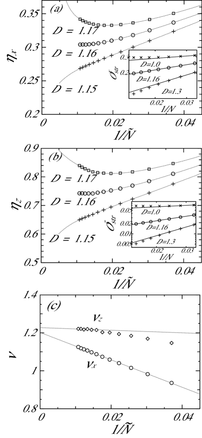
Figure 5: GSPRG analysis of (a) $\eta_{x}$, (b) $\eta_{z}$, and (c) $\nu_{\alpha}(D=1.16)$ on $J_{z}=1.25$. $\tilde{N}$ is given by Eq. (17). The dotted curves in (a) and (b) are guides for the eyes. The dotted lines in (c) are linear fitting lines. The string correlation functions $O^{x}_{\rm str}(N,D,J_{z}=1.25)$ and $O^{z}_{\rm str}(N,D,J_{z}=1.25)$ as a function of $1/N$ are shown in the logarithmic scale in the inset figures of (a) and (b), respectively.

In Fig.5(a), we observe the critical-disordered boundary at $D=1.17,N^{\prime}=55.3$. The critical-ordered boundary is also observed at $D=1.15,N^{\prime}=45.5$. On the other hand, we obtain no boundaries defined in eqs. (22a)-(23b) in the case of $D=1.16$. This fact suggests that the critical region for finite-size systems in our study is realized around $D=1.16$ with a narrow width. In order to confirm whether the width shrinks or not as the system sizes increase, we examine the relationship between $N^{\prime}$ and $D$ so that the case is on the boundary. We obtain some of the critical-disordered boundaries at $(D=1.19,N^{\prime}=36.8)$, $(D=1.2,N^{\prime}=32.7)$, and $(D=1.21,N^{\prime}=29.8)$. We also obtain some of the critical-ordered boundaries at $(D=1.14,N^{\prime}=32.7)$, $(D=1.13,N^{\prime}=30.0)$, and $(D=1.12,N^{\prime}=29.1)$. These results indicate that the critical region for a given $N^{\prime}$ is gradually narrower when $N^{\prime}$ increases although the expression of the relationship between $N^{\prime}$ and $D$ on the boundary is unknown in the present stage. It is reasonable to conclude that the critical region shrinks and goes to the transition point for the infinite-size system. When one can confirm whether the critical region between the two boundaries is sufficiently narrow or not, the width of the region should be regarded as an error coming from the maximum system size and the interval of $D$ in the performed calculations. In this work, thus, we conclude $D^{\textrm{HL}}_{\textrm{c}}(J_{z}=1.25)=1.16\pm 0.01$. Note here that we can obtain the same critical point from $\eta_{z}$ in Fig.5(b) in the same manner. Hereafter, we determine critical points with an error in this way. In order to confirm whether the critical behavior (14b) or (16b) appears or not in the original correlation functions, each string correlation function as a function of $1/N$ is shown in the logarithmic scale in inset figures. The finite-size string correlations for each direction clearly reveal a power-law decay behavior at the critical point $D^{\textrm{HL}}_{\textrm{c}}(J_{z}=1.25)=1.16$. On the other hand, a behavior deviating from power-law decay appears in the cases of $D=1.0$ and $D=1.3$ in the ordered and disordered phases, respectively, as we have mentioned in §III.3. Note here that a comparison with these insets shows that the system size dependence of the finite-size quantity (17) sensitively change near the transition point. We next observe the $\tilde{N}$ dependence of the finite-size exponents of $\nu_{x}(\tilde{N},1.16,1.25)$ and $\nu_{z}(\tilde{N},1.16,1.25)$ for $J_{z}=1.25$ and $D^{\textrm{HL}}_{\textrm{c}}(J_{z}=1.25)=1.16$ in Fig.5(c). These two finite-size exponents, $\nu_{x}$ and $\nu_{z}$, get gradually closer with increasing $\tilde{N}$. In the limit $\tilde{N}\rightarrow\infty$, $\nu_{x}$ and $\nu_{z}$ appear to approach a single value $\sim$1.2. This is consistent with the above argument on the unique characteristic length. Consequently, the problem of the disagreement of $\nu_{x}$ and $\nu_{z}$ in the FSS analysis occurs due to the finite-size effect and is resolved by GSPRG analysis.

We now consider the transition point $D_{\rm c}$ for a fixed $J_{z}=1$. In this case, many studies have reported various estimates for the boundary of the Haldane phase, $D_{\rm c}$: $D_{\rm c}=0.93\pm 0.02$ in Ref. Sakai_Takahashi:PRB42 , $D_{\rm c}=0.99\pm 0.02$ in Ref. Golinelli:PRB46 , $D_{\rm c}=0.90\pm 0.05$ in Ref. Tonegawa:JPSJ65 , $D_{\rm c}=1.001\pm 0.001$ in Ref. Chen:JPSJ69 , $D_{\rm c}=0.95$ in Ref. Koga:PL296 , $D_{\rm c}=0.99$ in Ref. Boschi:EPJB35 , and $D_{\rm c}\sim 0.97$ in Ref. Tzeng:PRA77 . Among these works, only a single study Tonegawa:JPSJ65 was based on the analysis of the string order, although data from the numerical-diagonalization calculations in this study for small clusters might not be sufficient to show the transition point. Recently, Tzeng and Yang Tzeng:PRA77 investigated the fidelity susceptibility Venuti:PRL99 of the ground state by the DMRG method to detect quantum phase transitions for the system. This work examines only the information of the ground state, a feature that is shared with our present analysis. Other works analyzed the structure of low-energy levels. From the present analysis, our estimate is $D_{\rm c}=0.975\pm 0.015$, which we have obtained irrespective of $\alpha=x$ or $\alpha=z$. Although the estimates are all very close to each other, there are small differences between them even taking errors into account. The reason for these differences is not clear at present and should be resolved as a future issue.

Next, we consider the transition point $D_{\rm c}$ for a fixed $J_{z}=0.5$. The estimation of this point is suitable for checking the availability of our analysis procedure, because a relatively large exponent $\nu$ which is reported 2.38 by analysis of the energy level structure appears Boschi:EPJB35 . Several previous studies presented numerical data of the transition point as follows: $D_{\rm c}=0.635$ in Ref. Hida:PRB67 , $D_{\rm c}=0.65$ in Ref. Boschi:EPJB35 , $D_{\rm c}=0.633\pm 0.02$ in Ref. Roncaglia:PRB77 . All of these works examined the free energy near the critical point to determine the critical point. In particular, the recent study Roncaglia:PRB77 develops rapidly converging methods by using the differentiations of a quantity, which is derivative of the ground state energy with respect to a controlled parameter, as a function of $N$. From the viewpoint of using only information in the ground state for detecting a quantum phase transition, our analysis and their analysis have a common policy. Our estimate for $D_{\rm c}(J_{z}=0.5)$ is $0.67\pm 0.04$, and this estimate is also consistent with all previous reports.

In accordance with the above results, we apply the procedure to estimate the critical behavior for other $J_{z}$, confirming the $J_{z}$ dependence of $D^{\textrm{HL}}_{\textrm{c}}(J_{z})$ and $\nu(D^{\textrm{HL}}_{\textrm{c}},J_{z})$. The error of $\nu(D^{\textrm{HL}}_{\textrm{c}},J_{z})$ is estimated by $|\nu(D^{\textrm{HL}}_{\textrm{c}},J_{z})-\nu(D^{\tilde{N}=93,\textrm{HL}}_{\textrm{c}},J_{z})|$. We illustrate our results in Fig. 6 together with those of previous reports Chen:JPSJ69 ; Hida:PRB67 ; Boschi:EPJB41 .

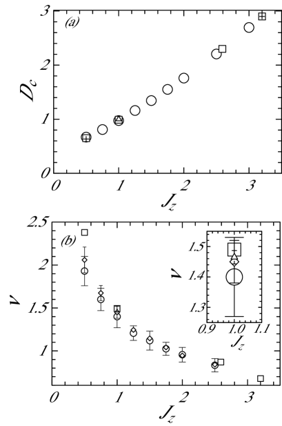
Figure 6: (a) Haldane–Large-$D$ transition line and (b) critical exponent $\nu_{\alpha}(J_{z})$. $\bigcirc$: evaluated value of x-component, $\Diamond$: evaluated value of z-component, +: Ref. Hida:PRB67 , $\square$: Ref. Boschi:EPJB41 , $\bigtriangleup$: Ref. Chen:JPSJ69 . The inset of (b) magnifies the data at $J_{z}=1$ to allow a clear comparison to distinguish the data.

Our estimates of $D^{\textrm{HL}}_{\textrm{c}}(J_{z})$ and $\nu(D^{\textrm{HL}}_{\textrm{c}},J_{z})$ are common for $\alpha=x$ and $\alpha=z$ within errors. Our transition line is almost consistent with those of previous reports Chen:JPSJ69 ; Hida:PRB67 ; Boschi:EPJB41 , in which the energy-level structure is analyzed. Our estimates of $\nu$ also agree well with previous reports within errors. Consequently, our GSPRG analysis successfully captures the transition between the Haldane phase and the large-$D$ phase.

The correlation length exponent $\nu$ is known to be related to other critical exponents. In the Gaussian transition, Okamoto obtained the following relationship from the argument by the bosonization method:

$$\nu=\frac{2}{4-\eta^{z}_{\rm N\acute{\textrm{e}}el}},$$ (29)

where $\eta^{\alpha}_{\rm N\acute{\textrm{e}}el}$ is the exponent defined by $\langle S_{0}^{\alpha}S_{r}^{\alpha}\rangle\sim(-1)^{r}r^{-\eta^{\alpha}_{\rm N\acute{\textrm{e}}el}}$ at the transition point. Note here that $\eta^{x}_{\rm N\acute{\textrm{e}}el}\eta^{z}_{\rm N\acute{\textrm{e}}el}=1$ holds. To confirm the consistency between our estimate of $\nu$ and the decay of the N$\acute{\textrm{e}}$el correlation function, we plot our $O_{\rm N\acute{\textrm{e}}el}^{x}(N,D,J_{z})$ at $J_{z}=1$ and $D_{\rm c}=0.975$ as a function of $1/N$ on a logarithmic scale in Fig. 7. We clearly observe a linear behavior for large $N$. We have added the dotted line $O_{\rm N\acute{\textrm{e}}el}^{x}(N,D,J_{z})\propto N^{-\eta^{x}_{\rm N\acute{\textrm{e}}el}}$ with $\eta^{x}_{\rm N\acute{\textrm{e}}el}=0.40$. From Eq. (29), this value of $\eta^{x}_{\rm N\acute{\textrm{e}}el}(=1/\eta^{z}_{\rm N\acute{\textrm{e}}el})$ gives $\nu\sim 1.33$, which is consistent with our estimate shown in the inset of Fig. 6. This consistency also supports the scaling hypothesis that the growth of the unique correlation length determines all the critical behavior around the transition point.

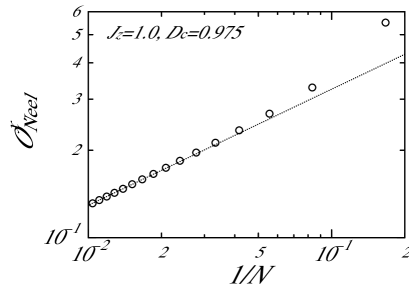
Figure 7: $1/N$ dependence of $O_{\rm N\acute{\textrm{e}}el}^{x}(N,D,J_{z})$ at $J_{z}=1$ and $D_{\rm c}=0.975$. The dotted line shows $O_{\rm N\acute{\textrm{e}}el}^{x}(N,D,J_{z})\propto N^{-\eta^{x}_{\rm N\acute{\textrm{e}}el}}$ with $\eta^{x}_{\rm N\acute{\textrm{e}}el}=0.40$.

IV.3 Haldane–N$\acute{\textrm{e}}$el transition line

In this subsection, we examine the transition from the Haldane phase to the N$\acute{\textrm{e}}$el phase. This transition is considered to be of Ising type. We recall that in a transition of Ising type, the exponent of the correlation length is $\nu=1$ when the system approaches the transition point.

We have mentioned in the above that the longitudinal string order is nonzero in both of the Haldane phase and the N$\acute{\textrm{e}}$el phase and that the order does not reveal the critical behavior at the transition point. This means that the longitudinal string order is not appropriate for studying the Haldane–N$\acute{\textrm{e}}$el transition. Therefore, to study this transition we examine only the transverse string order. By GSPRG analysis of this order, we determine the transition point $J_{z}^{\textrm{c}}$ for a given $D$ or the transition point $D_{\rm c}$ for a given $J_{z}$ and the critical exponent $\nu$ near the transition point.

We consider the case of $D=0.5$. We illustrate our result for finite-size exponents $\eta_{x}$ and $\nu$ in Fig. 8(a) and (b), respectively.

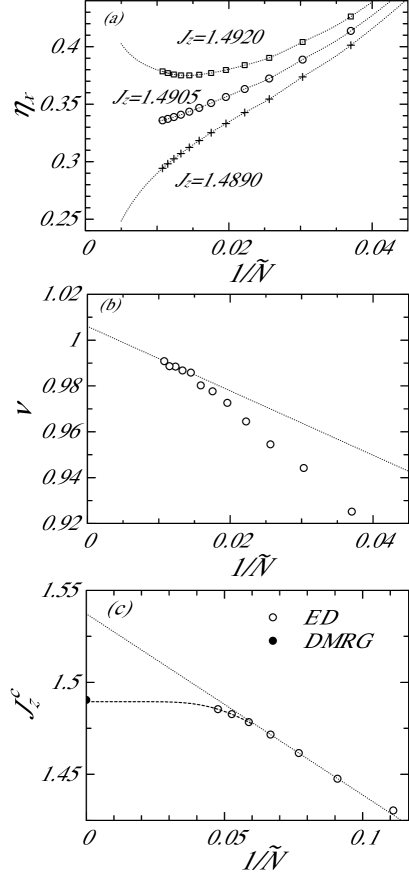
Figure 8: GSPRG analysis of (a) $\eta_{x}$ and (b) $\nu(J_{z}=1.4905)$ for $D=0.5$ from our DMRG results for $\Delta N=6$. The dotted curves in (a) are guides for the eyes. The dotted line in (b) is a linear fitting line applied to the data for large $\tilde{N}$. (c) Extrapolation procedure of the finite-size critical point $J^{\textrm{c}}_{z}$ for $D=0.5$ by the numerical-diagonalization method for $\Delta N=2$. The numerical-diagonalization data for $\tilde{N}=17,19,21$ are new in this paper. The dotted line is the extrapolation line in Ref. Hida:PRB67 . The broken curve is a guide for the eyes.

Our estimates are $J^{\textrm{c,HN}}_{z}(D=0.5)=1.4905\pm 0.0015$ and $\nu(J_{z}=1.4905,D=0.5)=1.006\pm 0.016$. Our estimate of the transition point is different from that of $J^{\textrm{c,HN}}_{z}(D=0.5)=1.536$ reported in Ref. Hida:PRB67 . To find the reason for the difference between the two estimates, we have made numerical-diagonalization calculations of finite-size clusters up to $N=22$ under the periodic boundary condition and obtained the eigenenergies of the low-energy states. We have performed the same analysis as that in Ref. Hida:PRB67 and determined the finite-size critical point $J^{\textrm{c,HN}}_{z}(\tilde{N},D=0.5)$ as $J_{z}$ at which the scaled energy gap does not depend on the system size for $\Delta N=2$. The results are depicted in Fig. 8(c). From our numerical data for $N=8,10,\cdots,16$, we successfully reproduce the results of Ref. Hida:PRB67 . On the other hand, we can observe that $J^{\textrm{c,HN}}_{z}(\tilde{N},D=0.5)$ of $\tilde{N}=17,19,21$ gradually departs from the fitting line of the extrapolation in Ref. Hida:PRB67 . Our new data points approach our estimates from the string order by the DMRG calculations, as shown by the guide for the eyes denoted by the broken curve in Fig. 8(c). This agreement suggests that the results from the numerical-diagonalization and DMRG calculations are consistent with each other if we accept the interpretation suggested by the broken curve. Hence, careful extrapolation with respect to system size is required.

The $\tilde{N}$ dependence of our new data appears exponential rather than polynomial. A similar $\tilde{N}$ dependence of $J^{\textrm{c,HN}}_{z}(\tilde{N},D=1)$ was reported in Ref. Boschi:EPJB41 , in which calculations up to $N=48$ based on the multi-target DMRG method with an infinite-system algorithm were carried out under the periodic boundary condition. Our result and Ref. Boschi:EPJB41 suggest that the absence of polynomial components does not depend on the values of the parameters of the system. It is important to be careful when a system-size extrapolation of an Ising transition point is carried out by the PRG analysis of the energy-level structure.

We now compare estimates of the transition point between Ref. Boschi:EPJB41 and the present analysis. Reference Boschi:EPJB41 gives $J^{\textrm{c, HN}}_{z}(D=0)=1.186$. From the present analysis of our data up to $N=150$, we obtain $J^{\textrm{c, HN}}_{z}(D=0)=1.1860\pm 0.0003$ for the transition point. Our estimate, with a very small error, agrees excellently with the estimate in Ref. Boschi:EPJB41 .

We now discuss our estimate of $\nu$. Our estimate $\nu(J_{z}=1.4905,D=0.5)=1.006\pm 0.016$ is in good agreement with $\nu=1$ of the Ising-type transition. This agreement also suggests that our analysis successfully captures the Haldane–N$\acute{\textrm{e}}$el transition as well as the Haldane–Large-$D$ transition.

We can now summarize our results for the transition points $D_{\rm c}$ for a given $J_{z}$ and the critical exponents $\nu$ between the Haldane and the N$\acute{\textrm{e}}$el phases from our DMRG data. The results are depicted in Fig. 9.

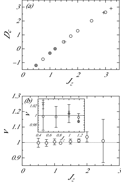
Figure 9: (a) Haldane–N$\acute{\textrm{e}}$el transition points. $\bigcirc$: Our work, +: Ref. Hida:PRB67 , $\Diamond$: Ref. Boschi:EPJB41 . (b) Haldane–N$\acute{\textrm{e}}$el critical exponent $\nu$. The inset figure compares our $\nu$ with that of Ref. Boschi:EPJB41 .

Figure 9(a) shows that our estimates for the transition points are in good agreement with the results in Ref. Boschi:EPJB41 of the multi-target DMRG method and the results in Ref. Hida:PRB67 of the numerical diagonalizations. In Fig. 9(b), our estimates for the exponent agree well with $\nu=1$ irrespective of $J_{z}$. Note here that the center values of our estimates, namely the extrapolated results, are much closer to $\nu=1$ than the results in Ref. Boschi:EPJB41 , although our errors are estimated to be larger. Note also that the error in $\nu(D^{\textrm{HN}}_{\textrm{c}}=2.015,J_{z}=2.5)$ is quite large. The reason for this is considered to be that the curve of the Haldane–N$\acute{\textrm{e}}$el transition points and that of the Haldane–Large-$D$ transition points approach each other. A similar phenomenon appears when the central charge $c$ on the curve of the Haldane–Large-$D$ transition points was estimated in Ref. Hida:PRB67 , in which the estimate of $c$ gradually deviates from $c=1$ around $J_{z}\gtrsim 1$. In the report of Tzeng and Yang Tzeng:PRA77 , the transition point and the critical exponent are given as $Dc^{\rm HN}(J_{z}=1)\sim-0.31$, $\nu(D^{\textrm{HN}}_{\textrm{c}}=-0.31,J_{z}=1.0)\sim 1.05$, respectively, from fidelity susceptibility analysis. Our estimated values at the same point are $Dc=-0.315\pm 0.003$, $\nu=1.004\pm 0.019$, which are more precise than the values of Tzeng and Yang.

IV.4 Haldane–$XY$ transition line

In this subsection, we examine the transition from the Haldane phase to the $XY$ phase. This transition is considered to be a BKT-type transition. We recall that in a BKT-type transition, the exponents $\eta_{x}=1/4$ and $\eta_{z}=1$ appear at the transition point and the exponent $\nu$ cannot be defined because the correlation length grows exponentially.

We consider the case $J_{z}<0$ and examine the magnitudes of the string order and the N$\acute{\textrm{e}}$el order. We refer back to the behavior of orders characterizing the Haldane phase, in which we have

$$|O^{z}_{\textrm{str}}|>0\mbox{ and }|O^{x}_{\textrm{str}}|>0,$$ (30)

under the condition

$$O^{x}_{\textrm{N}\acute{\textrm{e}}\textrm{el}}=O^{z}_{\textrm{N}\acute{\textrm{e}}\textrm{el}}=0.$$ (31)

This means that the region

$$|O^{\alpha}_{\textrm{str}}|\leq|O^{\alpha}_{\textrm{N}\acute{\textrm{e}}\textrm{el}}|,$$ (32)

is not in the Haldane phase because the inequality (30) and Eq. (31) cannot both be satisfied at the same time assuming the inequality (32). However, it is not as easy to make a direct comparison of these quantities in the limit $N\rightarrow\infty$ as for the inequality (32). We can instead compare the finite-size quantities $|O^{\alpha}_{\textrm{str}}(N,D,J_{z})|$ and $|O^{\alpha}_{\textrm{N}\acute{\textrm{e}}\textrm{el}}(N,D,J_{z})|$. Recall that for $N=300$, $|O^{\alpha}_{\textrm{str}}(N,D,J_{z})|$ is smaller than $|O^{\alpha}_{\textrm{N}\acute{\textrm{e}}\textrm{el}}(N,D,J_{z})|$ when $J_{z}<0$, whereas $|O^{\alpha}_{\textrm{str}}(N,D,J_{z})|$ is larger than $|O^{\alpha}_{\textrm{N}\acute{\textrm{e}}\textrm{el}}(N,D,J_{z})|$ when $J_{z}>0$. We have studied the system size dependence of this behavior; our results are depicted in Fig. 10.

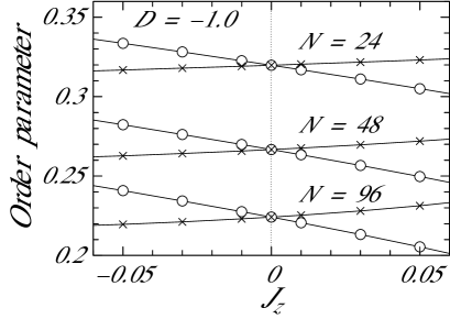
Figure 10: Order parameters crossing at $D=-1.0$. $\bigcirc$ and $\times$ represent $O^{x}_{\textrm{N}\acute{\textrm{e}}\textrm{el}}$ and $O^{x}_{\textrm{str}}$.

The behavior is clearly independent of system size. We can also confirm this independence irrespective of $D$ for cases between the Haldane phase and the $XY$ phase. Our present results suggest the inequality (32) and indicate that the Haldane–$XY$ transition point satisfies $J^{\textrm{c,HXY}}_{z}(D)\geq 0$. The finding is entirely consistent with previous works. Thus, it is sufficient to consider the case of $J_{z}\geq 0$ hereafter in examining the Haldane–$XY$ transition.

We now estimate $J^{\textrm{c,HXY}}_{z}$ by our GSPRG analysis. We consider the case $D=-0.5$ for $J_{z}\geq 0$. For this purpose, we examine the finite-size exponent $\eta_{\alpha}(\tilde{N},D=-0.5,J_{z})$, and estimate the critical-ordered boundary point $\eta_{\alpha}^{(1)}(N^{\prime},D=-0.5,J_{z})$ given by Eq. (23a) or Eq. (23b). Our results are depicted in Fig. 11.

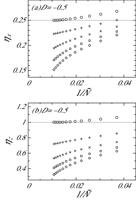
Figure 11: GSPRG analysis of the exponent $\eta_{\alpha}(\tilde{N},D=-0.5,J_{z}=0)$. The dotted lines are the rigorous exponent values of the BKT transition: $\eta_{x}=0.25$, $\eta_{z}=1$. $\bigcirc$, +, $\times$, $\square$, and $\Diamond$ represent $J_{z}=0$, 0.1, 0.15, 0.18, and 0.2, respectively.

We find that the critical-ordered boundary given by Eq. (23b) appears when $J_{z}$ is 0.1, 0.15, 0.18, and 0.2, but it does not appear when $J_{z}$ is 0. Concerning with $x$-component of the string order, we find the boundaries at $(J_{z}=0.18,N^{\prime}=29.6)_{x}$, $(J_{z}=0.15,N^{\prime}=31.0)_{x}$, and $(J_{z}=0.1,N^{\prime}=34.6)_{x}$. Concerning with $z$-component of the string order, on the other hand, we have $(J_{z}=0.18,N^{\prime}=32.6)_{z}$, $(J_{z}=0.15,N^{\prime}=35.2)_{z}$, and $(J_{z}=0.1,N^{\prime}=41.3)_{z}$ as the boundaries. In the cases of both of the components, one can observe that $N^{\prime}$ grows when $J_{z}$ approaches $J_{z}=0$. These phenomena lead to our result that $J^{\textrm{c,HXY}}_{z}$ is between $J_{z}=0$ and $J_{z}=0.1$. For estimating the transition point more accurately, the critical-ordered boundary point is extrapolated to the limit $N^{\prime}\rightarrow\infty$. The results are depicted in Fig. 12.

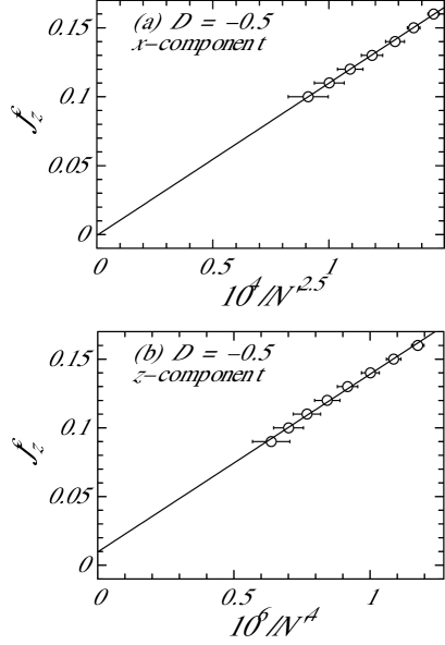
Figure 12: Behavior of the critical-ordered boundary point $J^{\textrm{c, HXY}}_{z}$ at $D=-0.5$ as a function of the system size $N^{\prime}$. Results are shown for $m_{\textrm{F}}=150$. The error is estimated from the difference between the results for $m_{\textrm{F}}=100$ and for $m_{\textrm{F}}=150$.

Since the leading dependence of $J^{\textrm{c, HXY}}_{z}$ on $1/N^{\prime}$ is unknown, we here choose the power $1/N^{\prime}$ so that the dependence is almost linear. We can successfully determine an appropriate value of the power for each $\alpha=x$ and $\alpha=z$, although the $\alpha=x$ and $\alpha=z$ values differ from each other. A linear extrapolation gives $J^{\textrm{c,HXY}}_{z}(D=-0.5)=0.00\pm 0.10$ from the transverse component and $J^{\textrm{c,HXY}}_{z}(D=-0.5)=0.01\pm 0.08$ from the longitudinal component. Here we determine the error as being the difference between the values obtained by the extrapolation and the finite-size critical point $J^{\textrm{c, HXY}}_{z}$ for maximum $N^{\prime}$. Both results suggest $J^{\textrm{c,HXY}}_{z}(D=-0.5)\sim 0$ irrespective of the direction of the string order parameter, which is consistent with a previous report Hida:PRB67 .

Next, we examine what type of transition this is. Our finite-size exponents in Fig. 11 at $J_{z}=0$ indicate $\eta_{x}(D=-0.5,J_{z}=0)\sim 0.25$ and $\eta_{z}(D=-0.5,J_{z}=0)\sim 1.0$. These values agree well with the exponents of the BKT transition $\eta_{x}=1/4$ and $\eta_{z}=1$. Our results are also consistent with many previous works Alcaraz:PRB46-2 ; Alcaraz:PRB46 ; Nomura:JPA28 ; Hida:PRB67 . Therefore, our GSPRG analysis applied to the string correlation functions is useful in capturing BKT transitions.

V summary and remarks

We have investigated critical behavior near the boundary of the Haldane phase in the ground state of an anisotropic $S=1$ chain from the viewpoint of string correlation functions estimated precisely by standard finite-size DMRG under the open boundary condition. We have developed the ground-state phenomenological-renormalization-group analysis and used it to analyze the correlation functions. This analysis provides us with the transition point of the boundary of the Haldane phase and the critical exponents at and near the transition point. Our estimates for these quantities agree with those previously obtained from analysis of the energy-level structure.

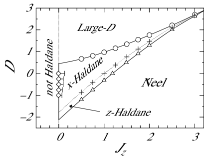
Figure 13: Phase diagram for the Hamiltonian (1). The Haldane–Large-$D$, Haldane–N$\acute{\textrm{e}}$el, and Haldane–$XY$ transition points are denoted by $\bigcirc,\triangle,\Diamond$, respectively. All the lines are guides for the eyes. x-Haldane and z-Haldane represent the $O^{x}_{str}>O^{z}_{str}$ region and $O^{x}_{\textrm{str}}<O^{z}_{\textrm{str}}$ regions, respectively.

We summarize the transition points as a ground-state phase diagram in Fig. 13. This figure presents the phase boundary of the Haldane–Large-$D$, Haldane–N$\acute{\textrm{e}}$el, and Haldane–$XY$ transitions. Note additionally that the dominant order parameter is $O^{x}_{\textrm{str}}$ in most of the Haldane phase.

A feature of our approach, GSPRG analysis, is that only common quantities under the same condition are treated in a unified manner irrespective of the type of phase transition. Although we have employed the DMRG method in this paper to calculate the order parameters, we are not limited to the DMRG method if we can obtain precise estimates of the order parameters. The string order parameters of the Haldane phase in the $S=1$ chain are examples. Other multi-point correlation functions for finite-size clusters may also be applicable. If we precisely calculate an appropriate ground-state quantity that plays the role of an order parameter, the framework of the analysis would be widely applicable for capturing ground-state critical behavior irrespective of the method of calculation and the kind of order parameter. We hope that the procedure presented in this paper contributes to future studies of quantum phase transitions.

- (1) M. N. Barber, In ”Phase Transitions and Critical Phenomena”, Vol. 8, (C. Domb and M. S. Green, eds.), Academic Press, London, p. 145, (1983).
- (2) J. M. Kosterlitz, J. Phys. C, 7, 1046 (1974).
- (3) K. Nomura, J. Phys. A 28, 5451 (1995).
- (4) S. R. White, Phys. Rev. Lett. 69, 2863 (1992).
- (5) S. R. White, Phys. Rev. B 48, 10345 (1993).
- (6) F. D. M. Haldane, Phys. Lett. 93A, 464 (1983).
- (7) F. D. M. Haldane, Phys. Rev. Lett. 50, 1153 (1983).
- (8) F. C. Alcaraz and Y. Hatsugai, Phys. Rev. B 46, 13914 (1992).
- (9) W. Chen, K. Hida, and B. C. Sanctuary, Phys. Rev. B 67, 104401 (2003).
- (10) C. D. E. Boschi, E. Ercolessi, F. Ortolani, and M. Roncaglia, Eur. Phys. J. B 35, 465 (2003).
- (11) C. D. E. Boschi and F. Ortolani, Eur. Phys. J. B 41, 503 (2004).
- (12) M. den Nijs and K. Rommelse, Phys. Rev. B 40, 4709 (1989).
- (13) T. Kennedy and H. Tasaki, Phys. Rev. B 45, 304 (1992).
- (14) K. Totsuka, Y. Nishiyama, N. Hatano, and M. Suzuki, J. Phys: Condens. Matter 7, 4895 (1995).
- (15) T. Tonegawa, T. Nakao, and M. Kaburagi, J. Phys. Soc. Jpn. 65, 3317 (1996).
- (16) Y. Hatsugai and M. Kohmoto, Phys. Rev. B 44, 11789 (1991).
- (17) S. Tonooka, H. Nakano, K. Kusakabe, and N. Suzuki, J. Phys. Soc. Jpn. 76, 084714 (2007).
- (18) S. R. White, Phys. Rev. Lett. 77, 3633 (1996).
- (19) An estimation of string correlation functions with periodic boundary condition by the DMRG method has been reported Boschi:EPJB41 . However, the result for correlation functions is translationally non-invariant in spite of the fact that the system is translationally invariant. Under such circumstances, it is difficult to capture the phase transition precisely if we examine the correlation function of the longest distance between and .
- (20) K. Hida, J. Phys. Soc. Jpn. 62, 1466 (1993).
- (21) T. Kennedy and H. Tasaki, Commun. Math. Phys. 147, 431 (1992).
- (22) T. Sakai and M. Takahashi, Phys. Rev. B 42, 4537 (1990).
- (23) O. Golinelli, T. Jolicoeur, and R. Lacaze, Phys. Rev. B 46, 10854 (1992).
- (24) A. Koga, Phys. Lett. 296, 243 (2002).
- (25) W. Chen, K. Hida, and B. C. Sanctuary, J. Phys. Soc. Jpn. 69, 237 (2000).
- (26) Y.C. Tzeng and M.F. Yang, Phys. Rev. A 77, 012311 (2008).
- (27) L. Campos Venuti and P. Zanardi, Phys. Rev. Lett. 99, 095701 (2007).
- (28) M. Roncaglia, L. Campos Venuti, and C. Degli Esposti Boschi, Phys. Rev. B 77, 155413 (2008).
- (29) K. Okamoto, J. Phys. A 29, 1639 (1996).
- (30) F. C. Alcaraz and A. Moreo, Phys. Rev. B 46, 2896 (1992).