Seismology of $\beta$ Cephei stars: differentially-rotating models for interpreting the oscillation spectrum of $\nu$ Eridani

Abstract

A method for the asteroseismic analysis of $\beta$ Cephei stars is presented and applied to the star $\nu$ Eridani. The method is based on the analysis of rotational splittings, and their asymmetries using differentially-rotating asteroseismic models. Models with masses around $7.13\,{\mathrm{M}_{\odot}}$, and ages around 14.9 Myr, were found to fit better 10 of the 14 observed frequencies, which were identified as the fundamental radial mode and the three $\ell=1$ triplets ${\rm g}_{1}$, ${\rm p}_{1}$, and ${\rm p}_{2}$. The splittings and aymmetries found for these modes recover those provided in the literature, except for ${\rm p}_{2}$. For this last mode, all its non-axysimmetric components are predicted by the models. Moreover, opposite signs of the observed and predicted splitting asymmetries are found. If identification is confirmed, this can be a very interesting source of information about the internal rotation profile, in particular in the outer regions of the star.

In general, the seismic models which include a description for shellular rotation yield slightly better results as compared with those given by uniformly-rotating models. Furthermore, we show that asymmetries are quite dependent on the overshooting of the convective core, which make the present technique suitable for testing the theories describing the angular momentum redistribution and chemical mixing due to rotationally-induced turbulence.

1 Introduction

The $\beta$ Cephei star $\nu$ Eridani (HD 29248 (catalog )) is nowadays one of the most in-depth studied stars. Classified as a B2III star, it presents a relatively simple internal structure, characterised by a large convective core. The $\kappa$ mechanism located in the metal opacity bump situated around $2\times 10^{5}\,\mathrm{K}$ (Dziembowski & Pamiatnykh, 1993; Gautschy & Saio, 1993), drives its oscillations. In addition, the pulsation periods of $\beta$ Cephei stars, varying in the range of 3–8 hours, makes them suitable for detecting and analysing oscillation frequencies. Several photometric and spectroscopic multisite observational campaigns for $\nu$ Eridani have been set up since 2002 with subsequent frequency analysis from spectroscopy (Aerts et al., 2004) and from photometry (Handler et al., 2004; Jerzykiewicz, et al., 2005). In these later works, two independent low-frequency, high-order ${\rm g}$ modes were detected. As a consequence, $\nu$ Eridani can also be classified as a SPB star. In terms of light curves, these multisite observations constitute the largest time-series ever collected for a $\beta$ Cephei star. Nowadays, $\nu$ Eridani presents the richest oscillation spectrum (14 independent frequencies) of the $\beta$ Cephei-type class. Such privileged scenario for asteroseismology has led to several authors to analyse its oscillation spectrum and perform seismic models of the star.

Several attempts have been carried out to provide a plausible seismic model which explains the observed frequencies of $\nu$ Eridani. In Ausseloos et al. (2004) (hereafter ASTA04), a massive exploration of standard and non-standard stellar models was undertaken in order to fit the oscillation data. The authors showed that an increase in the relative number fraction of iron throughout the whole star, or a large decrease in the initial hydrogen abundance, made the stellar models satisfy all the observational constraints, in particular, the modes around the fundamental radial mode are predicted unstable.

Pamyatnykh et al. (2004) performed a seismic analysis of the oscillation spectrum of $\nu$ Eridani taking the excitation of modes into account. In that work only three frequencies were fitted, failing to reproduce mode excitation in the broad observed frequency range of the ($\ell=1,p_{2}$) modes, associated with the highest frequency peak in the spectrum. Nevertheless, they also inferred some properties of the internal rotation rate using the rotational splittings of two dipole ($\ell=1$) modes identified as ${\rm g}_{1}$ and ${\rm p}_{1}$. In particular, their results suggest that the mean rotation rate in the core and the $\mu$-gradient zone is about three times higher than in the envelope, for their two standard models fitting the three aforementioned frequencies.

Recently, Dziembowski & Pamyatnykh (2008) have analysed the impact of considering uncertainties in the opacity and element distributions on the interpretation of $\nu$ Eridani’s oscillation spectrum. No satisfactory explanation of the low-frequency modes was found. Moreover, the authors concluded that some enhancement of the opacity in the driving zone is required.

The rotational splitting asymmetries of $\nu$ Eridani have also been studied under different hypothesis. In particular, Dziembowski & Jerzykiewicz (2003) suggested that the asymmetry of the $\ell=1$ triplet (around $5.64\,{\rm d}^{-1}$), as measured by van Hoof, A. (1961), could be explained by two principal effects: the quadratic effects of rotation and a strong magnetic dipole field of the order of 5–10 kG. Such a magnetic field was searched for by Schnerr et al. (2006) using spectropolarimetry with no success.

Table 1: A list of independent frequencies taken from Jerzykiewicz, et al. (2005).

ID	$f_{i}$ [$\mathrm{d}^{-1}$]	$f_{i}$ [${\mu\mbox{Hz}}$]
$f_{1}$	5.7632828	66.7047
$f_{2}$	5.6538767	65.4384
$f_{3}$	5.6200186	65.0465
$f_{4}$	5.6372470	65.2459
$f_{5}$	7.898200	91.4143
$f_{6}$	6.243847	72.2667
$f_{7}$	6.262917	72.4875
$f_{8}$	7.20090	83.3437
$f_{9}$	7.91383	91.5952
$f_{10}$	7.92992	91.7815
$f_{11}$	6.73223	77.9193
$f_{12}$	6.22360	72.0324

Motivated by these results, the present work aims at performing a complete modelling of $\nu$ Eridani taking the effect of rotation up to second order into account, with the special feature of considering the presence of a radial differential rotation in the seismic modelling. To do so, a method based on the analysis of rotational splittings and their asymmetries is discussed.

The paper is organised as follows: Section 2 describes the modelling procedure and provide details of both the evolutionary models and the oscillation spectra computation. In Section 3, the different sources for constraining the stellar parameters are compared, which include a stability analysis. Then, Sections 4 and 5 explain the method here presented and discuss its application to the particular case of $\nu$ Eridani. Finally, conclusions and final remarks are written in Section 6.

2 Seismic modelling

The seismic modelling described below consists in the computation of evolutionary models and their corresponding adiabatic and non-adiabatic oscillation spectra. This is described in the following sections.

2.1 Equilibrium models

To theoretically characterise $\nu$ Eridani, we build equilibrium models representative of the star with the evolutionary code cesam (Morel, 1997). In particular, models taking first-order effects of rotation into account are constructed. Such models are the so-called pseudo-rotating models, whose spherically averaged contribution of the centrifugal acceleration is included by means of an effective gravity ${\rm g}_{\mathrm{eff}}=g-{\cal A}_{c}(r)$, where ${\rm g}$ is the local gravity, $r$ is the radius, and ${\cal A}_{c}(r)=2/3\,r\,\Omega^{2}(r)$ is the centrifugal acceleration of matter elements. This spherically averaged component of the centrifugal acceleration does not change the order of the hydrostatic equilibrium equations (Kippenhahn & Weigert, 1990). The non-spherical components of the centrifugal acceleration (which are not included in the equilibrium models), are included in the adiabatic oscillation computations (see next section) by means of a linear perturbation analysis according to Soufi, Goupil & Dziembowski (1998) (see also Suárez, Goupil & Morel 2006). It is possible to evaluate the impact of a differential rotation, using two simple hypothesis when prescribing the rotation profile (Suárez et al., 2006): 1) instantaneous transport of angular momentum in the whole star (global conservation) which thus yields a uniform rotation, or 2) local conservation of the angular momentum (shellular rotation), except in the convective core whose rotation is assumed to be rigid. In both cases, no mass loss is considered at any evolutionary stage, that is, the total angular momentum is assumed to be conserved. These hypothesis represent extreme cases, so reality is presumably somewhere in between. In fact, similar rotation profiles have been found when analysing the evolution of giant stars including rotationally induced mixing of chemical elements and transport of angular momentum (Maeder & Meynet, 2004).

Input physics have been adequately chosen for main sequence B stars. Particularly, for the mass range treated in this work ($7$–$13\,{\mathrm{M}_{\odot}}$), the CEFF equation of state (Christensen-Dalsgaard & Daeppen, 1992) is used, in which, the Coulombian correction to the classical EFF (Eggleton et al., 1973) has been included. The opacity tables are taken from the OPAL package (Iglesias & Rogers, 1996). For the metal mixture, the abundances given by Grevesse & Noels (1996) are used.

A weak electronic screening is assumed, which is valid in the evolutionary stages considered in this work (see Clayton, 1968, for more details). For adiabatic stellar models, the Eddington’s $T(\tau)$ law (grey approximation) is considered for the atmosphere reconstruction. For non-adiabatic stellar models, the atmospheres are reconstructed using the Kurucz equilibrium atmospheric models (Kurucz, 1993) from a specific Rosseland optical depth until the the last edge (around $\tau=10^{-3}$) of the star is reached.

Convection is treated with the mixing-length theory (Böhm-Vitense, 1958) which is parametrised with $\alpha_{\rm MLT}=l/H_{\rm p}$, where $l$ is the mean path length of the convective elements, and $H_{\rm p}$ is the pressure scale height. In addition, we use the overshoot parameter, defined as ${d_{\rm ov}}$ ($l_{\rm ov}$ being the penetration length of the convective elements).

The grid of equilibrium models has been constructed with steps of 0.002 dex, 0.01, and 0.05, in the metallicity $Z$, overshoot parameter ${d_{\rm ov}}$, and mass $M$, respectively.

Figure 1: Mass-Metallicity relation fitting the observed frequencies $f_{1}$ and $f_{4}$ obtained from three different codes: cles, granada package and warsaw-new jersey codes. Two comparisons are shown: 1) for models without overshooting (liège package, granada package & warsaw-new jersey) and 2) for models with ${d_{\rm ov}}=$0.2 and 0.3 (liège package, granada package).

2.2 Oscillations

Adiabatic eigenfrequencies of selected pseudo-rotating models described in the previous section have been computed with the oscillation code filou (see Tran Minh & Léon, 1995; Suárez, 2002). In this code, oscillation frequencies are obtained by means of a perturbative method taking into account up to second order effects of rotation. In the case of near-degenerate frequencies, i.e. when two or more frequencies are close to each other ($\omega_{nlm}\sim\omega_{n^{\prime}l^{\prime}m}$), the corrections for near degeneracy are included. As detailed in Suárez et al. (2006), the oscillations computation also takes into account the presence of a radial differential rotation profile under the form

$$\Omega(r)={\bar{\Omega}}\,\Big{(}1+\eta_{0}(r)\Big{)}$$ (1)

where ${\bar{\Omega}}$ represents the angular rotational velocity at the surface and $\eta_{0}(r)$ a radial function. This rotation profile is equivalent to the shellular rotation profile obtained with the pseudo-rotating models described in the previous section.

Concerning the instability computations, non-adiabatic theoretical observables are obtained using graco code (Moya et al., 2004). This code solves the stellar pulsation equation in a non-adiabatic non-rotating frame by dividing the star in two parts, 1) the interior, by means of the non-adiabatic equations described in Unno et al. (1989), and 2) the atmosphere, taking into account the interaction with the pulsation as prescribed by Dupret et al. (2002).

2.3 Comparison of numerical seismic packages

As it is widely known, in stellar modelling, and in particular, in the field of stellar seismology, the use of different codes with different numerical techniques, can be crucial for the correct interpretation of seismic data (see Moya et al., 2008). ASTA04 compared two seismic packages: the liège package, which comprises the evolutionary code cles (Scuflaire et al., 2007), plus the oscillation code losc (Boury et al., 1975), and the warsaw-new jersey package (by Dziembowski & Jerzykiewicz, 2003) which comprises the warsaw-new jersey code and its corresponding oscillation code. Following ASTA04, these codes are compared (through a mass-metallicity relation) with our seismic modelling package, the granada package, which is composed by the evolutionary code cesam (Morel, 1997), and the oscillation code graco  (Moya et al., 2007) and filou (Suárez et al., 2007), described in Sections 2.1 and 2.2, respectively. Hereafter, those three packages are called LP, WP, and GP, respectively.

Similarly as done in ASTA04, the mass $M$, metallicity $Z$, overshoot parameter ${d_{\rm ov}}$, and initial hydrogen content $X_{\rm i}$, are then varied such as to fit the two observed frequencies, $f_{1}$ and $f_{4}$ (Table 1) by using non-rotating models. This procedure yields a mass-metallicity relation for each ${d_{\rm ov}}$ value, which is compatible with the similar study described in ASTA04 (see Fig. 1). It is found that, under similar conditions, i.e. for a given metallicity, ${\alpha_{\rm MLT}}$ and ${d_{\rm ov}}$, GP predicts higher mass values, around $0.25\,{\mathrm{M}_{\odot}}$. These differences increase slightly when ${d_{\rm ov}}$ increases. Such a different behaviour can be explained by the different treatments of the overshooting implemented in the evolutionary codes. Indeed, for the overshooting description, the Liège evolutionary code only takes the density variations (in the overshooted region) into account, which slightly affects the temperature gradient, whereas cesam considers an additional restriction by imposing that the real temperature gradient must be equal to the adiabatic one, i.e. $\nabla=\nabla_{\rm ad}$. This would imply that, either transport of heat is purely radiative, or it is efficiently transported outwards from the stellar core through convective movements (as a result of the overshooting), respectively. This constitutes an interesting challenge for asteroseismology because the oscillation modes are sensitive to the physical description of the $\mu$-gradient zone.

Figure 2: HR diagram containing the two estimates for the effective temperature and luminosity (filled star symbols) adopted in this work for $\nu$ Eridani (more details in Section 3.1), with the corresponding photometric uncertainty boxes (shaded area). For illustration, three evolutionary tracks of 7.60, 7.13 and $7\,{\mathrm{M}_{\odot}}$, are also depicted. Those models have been computed using an initial hydrogen content of $X_{\rm i}=0.5$. The filled circle represents the selected model NR1, which predicts unstable and better fits the observed frequencies $f_{1}$, $f_{4}$, $f_{6}$, and $f_{9}$. More details Section 3.2.

3 Constraining stellar parameters

The modelling of any star entails the constraint of its stellar parameters. For doing so, the choice of the set of free parameters to be fixed generally depends on the observational material available. In the case of $\nu$ Eridani, the following space of free parameters was chosen

$${\cal P}={\cal P}\,(M,t,{d_{\rm ov}},Z;\Omega)\,$$

where $M$ is the stellar mass, $t$ the age, ${d_{\rm ov}}$ the overshooting parameter, $Z$ the metallicity, and $\Omega$ the angular rotational velocity. From photometric and spectroscopic observations, we search for an estimate of the star location in the HR diagram. This allows us to constrain the metallicity and to have an estimate of the evolutionary stage of the star. Stability analysis significantly reduces the region of the HR diagram in which representative models can be searched.

Then, the fitting of four of the observed frequencies permits to better constrain the mass, metallicity, evolutionary stage (age) and overshooting parameter of the star. The small observed ${\mathrm{v}\!\sin\!i}$ of $\nu$ Eridani allows the use of non-rotating models for this exercise. However, further model constraining makes it necessary to take the stellar rotation into account. In particular, seismic models including shellular rotation profiles are used (see Section 2). Finally, analysis of the rotationally-split modes and their asymmetries allows to make a refined search for representative models of the star.

3.1 Locating $\nu$ Eridani in the HR diagram

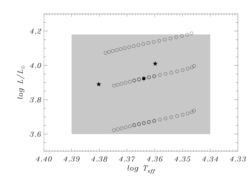
In order to locate the star in the HR diagram we followed the works by Morel et al. (2006) and De Ridder et al. (2004), based on high-precision spectroscopy. The error box shown in Fig. 2 takes into account the results reported in both papers.

Figure 3: Growth rates $\eta$ as a function of the oscillation frequency. Each curve represents the growth rate obtained for oscillation modes with different degree ($\ell$ ranging from 0 to 3). The lowest frequencies correspond to the SPB-type pulsation frequencies. Only the frequencies around the fundamental radial mode are predicted unstable (positive growth rate), which are those kept for the present investigation.

On the other hand, the location of stars in the HR diagram depends on both the rotational velocity of the star and the inclination angle with respect to the observer, $i$. A technique to estimate and correct for the effect of fast rotation on the determination of fundamental parameters for pulsating stars is described in Michel et al. (1999). This technique was then refined by Pérez Hernández et al. (1999), who applied it to $\delta$ Scuti stars in clusters. A first consequence that can be extracted from those works is that rotation increases the size of the uncertainty box of stars in the HR diagram (when obtained from photometry). In general, such additional uncertainties increase for increasing rotational velocities (for a given angle of inclination of the star). For $\nu$ Eridani, a projected rotational velocity of ${\mathrm{v}\!\sin\!i}\sim 16\,{\mathrm{km}\,\mathrm{s}^{-1}}$ has been observed. This value has been derived by Morel et al. (2006) from high-resolution spectroscopy, taking into account the broadening due to oscillations. In principle, it can be considered as a slow rotator so that the additional uncertainties coming from the effect of rotation can be considered within the already large photometric uncertainties.

Table 2: Characteristics of the best models selected in this work. The different columns are, from left to right: the model identification, the metallicity $Z$, the mass $M$, the radius $R$, the logarithm of the effective temperature ${T_{\mathrm{eff}}}$ (in K), the logarithm of the gravity $g$ (in cgs), the logarithm of the luminosity (cgs), the overshooting parameter (in the ${\rm H}_{p}$ scale), the rotational frequency of the surface ${\omega_{\rm s}}$ (in ${\mu\mbox{Hz}}$), the rotational frequency of the core ${\omega_{\rm c}}$ (in ${\mu\mbox{Hz}}$), the age (in Myr), the hydrogen abundance in the core ${X_{\rm c}}$, and the radius of the convective core ${r_{\rm c}}$.

Model	$Z$	${M/{\mathrm{M}_{\odot}}}$	${R/{\mathrm{R}_{\odot}}}$	${\log{T_{\mathrm{eff}}}}$	$\log g$	${\log(L/L_{\odot})}$	${d_{\rm ov}}$	${\omega_{\rm s}}$	${\omega_{\rm c}}$	Age	${X_{\rm c}}$	${{r_{\rm c}}/R}$
NR1	0.019	7.13	5.704	4.364	3.778	3.923	0.28	0	0	14.82	0.139	0.129
SR1	0.019	7.13	5.714	4.364	3.777	3.923	0.28	0.258	0.681	14.90	0.138	0.129
SR2	0.019	7.13	5.727	4.362	3.775	3.918	0.24	0.301	0.778	14.60	0.129	0.125
UR1	0.019	7.13	5.511	4.368	3.808	3.909	0.28	0.377	0.377	15.80	0.159	0.136

3.2 Instability predictions

Once the star is located in the HR diagram, models which predict the observed frequencies to be unstable (considering the constraints on physical parameters given above) are searched for.

To do so, no specific ad-hoc modification of the iron mixture throughout the star is proposed. The search for the best models is then enhanced by using the ${M-Z}$ relations presented in Section 2.3. We recall that lines in Fig. 1 represent the models which fit simultaneously both $f_{1}$ and $f_{4}$. These models constitute a first guess to the best solution. Finally, our best solution is given by those models that also fit $f_{6}$ and $f_{9}$. Consistently with ASTA04, when using standard solar mixture for the metallicity, an initial hydrogen content of $X_{\rm i}\sim 0.50$ is required in order to predict unstable the observed frequencies. In Fig. 2, the different evolutionary tracks shown have been computed using $X_{\rm i}=0.50$ in the ZAMS. From our grid of models (see Section 2.1), the best model (filled circle in Fig. 2) was selected to be the one which predicts unstable and better fits the observed frequencies $f_{1}$, $f_{4}$, $f_{6}$, and $f_{9}$. This best non-rotating model is characterised by a mass of $7.13\,{\mathrm{M}_{\odot}}$, a solar metallic mixture (with an initial hydrogen content of $X_{\rm i}=0.50$), and by the physical parameters ${\alpha_{\rm MLT}}=1$, $d_{\mathrm{ov}}=0.28$ (NR1 in Table 2). Note that rotation has not been taken into account in the instability predictions described above. The lack of theories describing the effect of rotation on mode stability makes it difficult to estimate this effect for $\nu$ Eridani. Nevertheless, as stated by Pamyatnykh (1975), mode stability depends predominantly on the effective temperature of the models (see Suárez et al., 2007, for an interesting discussion on this issue), whose variations due to rotation are expected to be small (due to the low rotational velocity of the star).

The results of the stability analysis obtained for that model are depicted in Fig. 3, in terms of growth rate as a function of the oscillation frequency. As expected, in the frequency region around the fundamental radial mode, the results obtained for the different spherical degrees $\ell$ are quite similar, which implies that this parameter cannot be discriminated.

4 Procedure

As discussed in Sections 2.1-2.2, the small rotational velocity of the star makes it plausible to initially adopt the parameters of the non-rotating models which were found to be representative of the star. In particular, in order to work with models located in the HR error box which predict unstable the observed frequencies, a value of $X_{\rm i}=0.5$ for the initial hydrogen fraction is kept (see previous section). Indeed, such a value is rather unrealistic. This can be solved either by considering an ad-hoc iron enhancement in the driving zone (as done by Pamyatnykh et al., 2004), or by modifying (uniformly throughout the stellar interior) the relative number fraction of iron (as done by ASTA04). However, the modelling techniques used here do not allow to make such modifications. Instead, following ASTA04 we simulate the metallicity change by modifying the initial hydrogen fraction. This yields, similarly to ASTA04 (see Table 1 in that paper), models around $7\,{\mathrm{M}_{\odot}}$ and $Z=0.018-0.019$. Similarly to previous works, standard models, i.e. those with $X_{\rm i}\sim 0.7$, within the HR error box present masses higher than $8\,{\mathrm{M}_{\odot}}$, $Z\sim 0.015$, for similar surface rotational velocities. Such variations with respect to the non-standard models have no significant impact neither on the rotation profile nor on the splitting asymmetries.

A systematic search for representative models within the error box was then performed locally varying the mass, initial rotational velocity, and age of the models. The mass was varied around $7.10\,{\mathrm{M}_{\odot}}$, in particular from 7 to $7.20\,{\mathrm{M}_{\odot}}$, in steps of $0.01\,{\mathrm{M}_{\odot}}$. Rotation was considered under two main assumptions: uniform rotation and differential rotation (see Section 2 for more details). For both assumptions, the rotational velocities considered range from to 5 to $20\,{\mathrm{km}\,\mathrm{s}^{-1}}$ at the stellar surface. Then, the modelling was refined by analysing the rotational splittings and their asymmetries. Rotational splittings are defined as

$$S=\frac{1}{2}\big{(}\nu_{+1}-\nu_{-1}\big{)}$$ (2)

and asymmetries of these splittings are defined as

$$A=\nu_{-1}+\nu_{+1}-2\nu_{0}\,.$$ (3)

where sub-indices $\pm 1$ represent the value of the azimuthal order $m$ for a given $\ell$. The information provided by the asymmetries can be completed by the semi-splittings, which corresponds with $\Delta^{+}=\nu_{+1}-\nu_{0}$, and $\Delta^{-}=\nu_{0}-\nu_{-1}$, respectively. Both quantities are related such as Eq. 3 transforms into

$$A=\Delta^{+}-\Delta^{-}\,.$$ (4)

Moreover, this analysis also permits to extract information about the internal rotation profile of the star, since, as we discuss in the next sections, $S$ and $A$ are both sensitive to changes in the rotation profile.

5 Results and discussion

Models with a mean density of about $\bar{\rho}=0.064\,{\rm g\,cm}^{-3}$ were found to fit better the observed frequencies. The models within $\pm 0.05\,{\mathrm{M}_{\odot}}$ of the mass value calibrated using non-rotating models yield similar results, but for slightly different ages. Due to the so small rotational velocity, it is plausible to assume the same ${\alpha_{\rm MLT}}$ and ${d_{\rm ov}}$ parameters which were calibrated by the non-rotating models. Therefore, only the mass, age, and initial rotational velocity of the models were varied.

Models were then selected to fit at least the observed frequencies $f_{1}$ (identified as the fundamental radial mode) and the triplet $(f_{3},f_{4},f_{2})$, identified as ${\rm g}_{1}$. With these criteria, a model with a mass of $7.13\,{\mathrm{M}_{\odot}}$, a rotational velocity (in the surface) of about $7\,{\mathrm{km}\,\mathrm{s}^{-1}}$, and an age of about 14.9 Myr (which corresponds with $\log{T_{\mathrm{eff}}}=4.365$) was found to better fit the observational frequencies. As expected, when rotation is taken into account, the stellar parameters of the models are similar to those of the non-rotating best model (NR1). For each type of rotation, i.e. uniform and shellular rotation, the models better matching the observed frequencies, splittings, and asymmetries, are UR1 and SR1, whose characteristics are summarised in Table 2 (their corresponding list of frequencies are reported in Table 3), and whose internal rotation profiles are depicted in Fig. 4. Figure 5 shows the evolution of the theoretical frequencies of the ${\rm g}_{1}$, ${\rm p}_{1}$ and ${\rm p}_{2}$ $\ell=1$ triplets for the selected model (assuming shellular rotation).

With these models, nine of the observed frequencies were identified as two $\ell=1$ triplets: a ${\rm g}_{1}$ triplet composed by the observed frequencies $(f_{3},f_{4},f_{2})$, a ${\rm p}_{1}$ triplet which corresponds with $(f_{12},f_{6},f_{7})$, and a ${\rm p}_{2}$ triplet which corresponds with $(f_{5},f_{9},f_{10})$. Furthermore, $f_{1}$ was identified as the fundamental radial mode. For the remaining frequencies ($f_{8}$ and $f_{11}$), the selected models present similar predictions. While $f_{8}$ is identified as a ($n=0,\ell=2$), all the models match $f_{11}$ with a $\ell\geq 7$ mode. In particular the best identification found corresponds to $(n,\ell,m)=(-3,9,8)$.

In general, these results are compatible with previous studies that can be found in the literature, except that we do identify and use (for asteroseismic purposes) all the non-axisymmetric components of the $\ell=1$ triplets, in particular ${\rm p}_{2}$. Differences with Dziembowski & Pamyatnykh (2008)’s work are principally related to this last split mode, whose identification depends strongly on the use of standard or non-standard models.

Table 3: List of theoretical frequencies (${\rm d}^{-1}$) for the three selected best models NR, SR1, SR2, and UR (see Table 2). The model A does not take rotation into account, hence only the frequencies of the $m=0$ components are reported.

Mode	$\nu_{{\rm NR},i}$	$\nu_{{\rm SR1},i}$	$\nu_{{\rm SR2},i}$	$\nu_{{\rm UR},i}$
F0	5.75818	5.74396	5.72332	5.77681
${\rm g}_{1,-1}$	-	5.65407	5.70359	5.66402
${\rm g}_{1,0}$	5.63699	5.63402	5.67979	5.64512
${\rm g}_{1,+1}$	-	5.61397	5.65585	5.62652
${\rm p}_{1,-1}$	-	6.26192	6.31067	6.27800
${\rm p}_{1,0}$	6.24442	6.24026	6.28685	6.25494
${\rm p}_{1,+1}$	-	6.21785	6.26212	6.23102
${\rm p}_{2,-1}$	-	7.89759	7.87980	7.94832
${\rm p}_{2,0}$	7.88829	7.87398	7.85263	7.91898
${\rm p}_{2,+1}$	-	7.84899	7.82361	7.88731

5.1 Analysis of rotational splittings and asymmetries

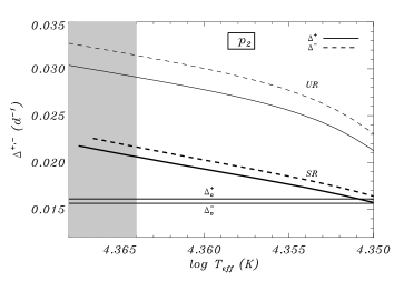
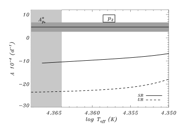
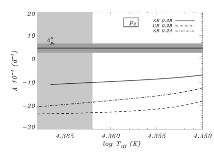
In Fig. 6, the predicted semi-splittings (left column) and asymmetries (right column), are compared with the corresponding observed values given in Table 4. For all panels in that figure, the shaded vertical regions indicate the range of ${T_{\mathrm{eff}}}$ values given by the best models SR1 and UR1 (see Table 2).

This comparison is performed simultaneously for models evolved assuming uniform and shellular rotation profiles (hereafter UR and SR models). For the sake of brevity, in the following, $A_{x}$, $A_{x}^{\rm o}$, are used to represent the predicted and observed asymmetries, $x$ representing the triplets ${\rm g}_{1}$, ${\rm p}_{1}$, or ${\rm p}_{2}$. Similarly, $\Delta^{+,-}$ and $\Delta_{\rm o}^{+,-}$ are used to represent the predicted and observed semi-splittings. Let us now examine each selected triplet separately.

5.1.1 The ${\rm g}_{1}$ triplet

Analysis of the ${\rm g}_{1}$ triplet (Fig. 6, left top panel) reveals that for the SR models, the predicted $|\Delta^{+}|$ remain lower than $|\Delta^{-}|$ for almost the whole range of effective temperature studied (almost identical in the shaded region). On the other hand, for UR models, $|\Delta^{-}|$ are predicted lower than $|\Delta^{+}|$ for effective temperatures higher than 23014 K ($\log{T_{\mathrm{eff}}}=4.362$), approximately. The deviation of the semi-splitting predictions (in the shaded region), defined as $\epsilon_{\Delta^{+,-}}=\Delta^{+,-}-\Delta^{+,-}_{\rm o}$, is about $2\times 10^{-3}\,{\rm d}^{-1}$ for the SR models and 3-$4\times 10^{-3}\,{\rm d}^{-1}$ for the UR models. On the other hand, cooler SR models would fit better the observations ($\epsilon_{\Delta^{+,-}}=10^{-6}\,{\rm d}^{-1}$ for models around $\log{T_{\mathrm{eff}}}=4.35$). In general, the evolution of the semi-splittings for both types of rotation is found to be quite different. This is somehow expected since ${\rm g}$ modes are very sensitive to variations of the rotational velocity of the core. In fact, it was shown by Suárez et al. (2006) that a shellular rotation profile modifies significantly the radial displacement eigenfunctions, especially for ${\rm g}$ and mixed modes. This implies that the presence of shellular rotation may affect both the rotational splitting itself and its asymmetry. The general definition of the first-order rotational splitting kernel can be written as

$${\cal K}=\displaystyle{{\Big{[}\big{(}2\,y_{01}z_{0}+z_{0}^{2}\big{)}+\eta_{0}\big{(}y_{01}^{2}+\Lambda z_{0}^{2}-2\,y_{01}z_{0}-z_{0}^{2}\big{)}\Big{]}\,\rho_{0}\,r^{4}}\over{{\displaystyle\int_{0}^{R}[y_{01}^{2}+\Lambda\,z_{0}^{2}]\,\rho_{0}\,r^{4}\,{\rm d}r}}},$$ (5)

where $\Lambda=\ell(\ell+1)$, and $y$ and $z$ represent the vertical and horizontal displacement normalised eigenfunctions, respectively. The second term within the square brackets accounts for the presence of shellular rotation through $\eta_{0}$, defined in Eq. 1. When a uniform rotation is considered, this term becomes null. In Fig. 7 such kernels are depicted for the ${\rm g}_{1}$, ${\rm p}_{1}$, and ${\rm p}_{2}$ triplets. Notice that, when considering a shellular rotation profile, a bump in the energy distribution near the $\mu$-gradient zone (see Fig. 4) comes up, for ${\rm g}_{1}$, at the expense of the energy of the outer layers, which could explain the different behaviour of the semi-splittings predicted by the UR and SR models.

Table 4: Observed semi-splittings, $(\Delta^{+},\Delta^{-})$, and asymmetries, $A^{\rm o}$ of the $\ell=1$ triplets ${\rm g}_{1}$, ${\rm p}_{1}$ and ${\rm p}_{2}$, as identified using a model of $7.13\,{\mathrm{M}_{\odot}}$ which rotates with $v\sim 5.5\,{\mathrm{km}\,\mathrm{s}^{-1}}$ in the surface. Quantities are given in ${\rm d}^{-1}$. Uncertainties, $\delta$, are calculated from data in Jerzykiewicz, et al. (2005).

Mode	$\Delta^{+}$	$\Delta^{-}$	$A^{\rm o}$
	$\delta(\Delta^{+})$	$\delta(\Delta^{-})$	$\delta(A^{\rm o})$
${\rm g}_{1}$	$0.016630$	$-0.01723$	$-0.000598$
	$\pm 6\times 10^{-6}$	$\pm 7\times 10^{-6}$	$\pm 1\times 10^{-5}$
${\rm p}_{1}$	$0.0191$	$-0.0203$	$-0.0012$
	$\pm 2\times 10^{-4}$	$\pm 2\times 10^{-4}$	$\pm 2\times 10^{-4}$
${\rm p}_{2}$	$0.0161$	$-0.0156$	$+0.0005$
	$\pm 1\times 10^{-4}$	$\pm 2\times 10^{-4}$	$\pm 2\times 10^{-4}$

Concerning the asymmetries, $A_{{\rm g}_{1}}$ are predicted to diminish for decreasing effective temperature (Fig. 6, right panel on top). In other words, asymmetries decrease while the star evolves. For UR models, such a decreasing is more rapid than for the SR models, and the asymmetries fit the observed value at $\log{T_{\mathrm{eff}}}\sim 4.357$, which represents a difference of $\sim 400\,$ K with respect to the models that fit the observed frequencies (shaded area). On the other hand, the asymmetries predicted by the SR models never fit exactly the observed value. In the shaded region, the deviation of the asymmetry defined as ${\epsilon_{A}}=A_{{\rm g}_{1}}-A_{{\rm g}_{1}}^{\rm o}$, is found to be $6\times 10^{-4}\,{\rm d}^{-1}$ for the SR models whereas for UR models ${\epsilon_{A}}=10^{-3}\,{\rm d}^{-1}$. Such deviations are respectively, two and three orders of magnitude larger than the observed asymmetry uncertainty.

As for the ${\rm g}_{1}$ semi-splittings, better results are found for cooler models, especially for UR models around $\log{T_{\mathrm{eff}}}=4.357$, and for SR models near $\log{T_{\mathrm{eff}}}=4.35$. In any case, for low order ${\rm g}$ and ${\rm p}$ modes, asymmetries are sensitive to variations of the rotation profile near the core. Indeed, as shown by Suárez et al. (2006), the analytical form of $A$ (using a perturbative theory) can be written as the second-order term

$$A=-{{6m^{2}}\over{4\Lambda-3}}{{{\bar{\Omega}}^{2}}\over{\omega_{0}}}{\cal J}_{c}\,.$$ (6)

where ${\bar{\Omega}}$ is the rotational velocity at the stellar surface, and $\omega_{0}$ is the unperturbed oscillation frequency. The ${\cal J}_{c}$ integral contains a complex combination of structure and oscillation terms which are modified by the rotation profile and its derivatives. Analysis of this term is definitely necessary to construct simplified kernels for $A$ (work in progress). Such kernels will help us to better understand the behaviour of the asymmetries, and, especially their sensitivity to variations of the internal rotation profile.

Figure 4: Rotation profile normalised to the rotation velocity in the surface, $\Omega_{\rm s}$, as a function of the normalised stellar radius, for the best SR model. For comparison, the rotation profile of UR model with similar $\Omega_{\rm s}$ is also depicted. For illustration purposes, the Brunt-Väisäla frequency for the SR model (re-scaled as to fit the plot) has been used to indicate the location of the $\mu$-gradient zone ($r\sim 0.15-0.2\,{\mathrm{R}_{\odot}}$).

5.1.2 The ${\rm p}_{1}$ triplet

For ${\rm p}_{1}$, the predicted curves of $|\Delta^{+}|$ remain lower than those of $|\Delta^{-}|$ in the whole range of effective temperature studied, which is compatible with the observations (Fig. 6, left middle panel). Notice that, in the shaded region, the SR models predict absolute values for the semi-splittings closer to the observed ones ($\epsilon_{\Delta^{+,-}}\sim 10^{-4}\,{\rm d}^{-1}$) than those predicted by the UR models, for which $\epsilon_{\Delta^{+,-}}=4\times 10^{-3}\,{\rm d}^{-1}$. However, this situation is reversed for the splitting asymmetries (Fig. 6, right middle panel). In particular, around $\log{T_{\mathrm{eff}}}=4.365$, the asymmetries predicted by the UR models (${\epsilon_{A}}=6\times 10^{-4}\,{\rm d}^{-1}$) are slightly closer to the observed values than those predicted by the SR models (${\epsilon_{A}}=2\times 10^{-4}\,{\rm d}^{-1}$). Even so, such differences are of the order of magnitude of the observational uncertainty of $A_{{\rm p}_{1}}$, which makes it difficult to discriminate between both types of rotation. Contrary to the ${\rm g}_{1}$ results, cooler models do not fit better the observations.

5.1.3 The ${\rm p}_{2}$ triplet

In the case of ${\rm p}_{2}$, the predicted semi-splittings are larger than the observed value in the whole range of effective temperatures, except for $\log{T_{\mathrm{eff}}}\sim 4.35$, for which SR predictions are almost coincident with the observations (Fig. 6, left bottom panel). In the shaded region $\epsilon_{\Delta^{+,-}}=6\times 10^{-3}\,{\rm d}^{-1}$ for the SR models and $\epsilon_{\Delta^{+,-}}=1.6\times 10^{-2}\,{\rm d}^{-1}$ for the UR models. Similarly to the ${\rm g}_{1}$ case, the best results are given by the SR models for effective temperatures around the cooler limit of the photometric uncertainty box ($\log{T_{\mathrm{eff}}}=4.35$).

Figure 5: Evolution of the theoretical oscillation frequencies corresponding, from to bottom, to the $\ell=1$ triplets ${\rm p}_{2}$, ${\rm p}_{1}$ and ${\rm g}_{1}$, for the selected $7.13\,{\mathrm{M}_{\odot}}$ model. Horizontal lines represent the observed frequencies, bottom to top, $f_{4}$, $f_{6}$, and $f_{9}$, identified as the $m=0$ components of the triplets ${\rm p}_{2}$, ${\rm p}_{1}$ and ${\rm g}_{1}$, respectively.

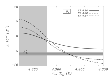
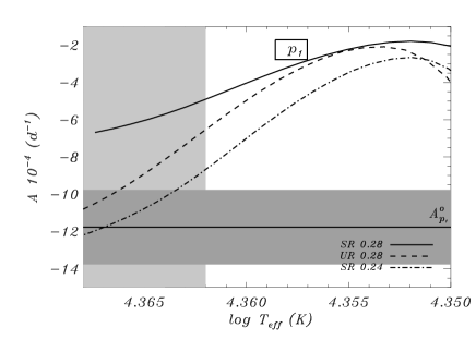
Furthermore, it is worth noting that contrary to the ${\rm p}_{1}$ and ${\rm g}_{1}$ cases, the observed semi-splitting $|\Delta^{-}|$ is smaller than $|\Delta^{+}|$, whereas both SR and UR models predict $|\Delta^{-}|>|\Delta^{+}|$ (Fig. 6, left bottom panel). This results in a positive observed asymmetry, whereas both UR and SR models predict negative values (Fig. 6, right bottom panel). In the vicinity of $\log{T_{\mathrm{eff}}}=4.365$ (shaded region), the difference between the observed and predicted asymmetries is about ${\epsilon_{A}}=10^{-3}\,{\rm d}^{-1}$ (${\epsilon_{A}}=1.5\times 10^{-3}\,{\rm d}^{-1}$ for the SR models and ${\epsilon_{A}}=2.8\times 10^{-3}\,{\rm d}^{-1}$ for the UR models), which represents a difference of one order of magnitude with respect to the observed value. Such apparently marginal contradiction between predictions and observations could be a consequence either of 1) an incorrect mode identification, that is, the observed frequencies concerned do not belong to the rotationally split mode, or 2) the use of a wrong description for the rotation profile, particularly in the outer shells of the star (note the small influence of the selected rotation profile near the $\mu$-gradient zone, Fig. 7). A priori, none of the these possibilities can be discarded. In order to solve this problem, improvements on both the observations and modelling are required. From the observational side, an improvement of accuracy with which the concerned observed frequencies are determined might help to confirm the observed asymmetry and its sign. Moreover, the detection of additional frequencies (e.g. with the help of space missions), may provide new insight on the current mode identification.

From the theoretical side, the second possibility given above is related with angular momentum redistribution, which plays an important role. In particular, balance between rotationally induced turbulence and meridional circulation generates mixing of chemicals and redistribution of angular momentum (Zahn, 1992), which affects the rotation profile and the evolution of the star. The present technique is, therefore, especially suitable for testing that theory by providing estimates for the coefficients of turbulence using only asteroseismic observables. This can be illustrated by artificially modifying the physical conditions beyond the convective core, which can be done varying the overshooting parameter.

Figure 6: Evolution of the theoretical semi-splittings (left column) and asymmetries (right column) as a function of the effective temperature (logarithmic scale) for the selected $7.13\,{\mathrm{M}_{\odot}}$ model with a rotational velocity of $7\,{\mathrm{km}\,\mathrm{s}^{-1}}$ , approximately. The observed values are depicted with horizontal lines, and the corresponding observational uncertainties are represented by horizontal shaded bands. Each panel row shows the results, from top to bottom, for the $\ell=1$ triplets ${\rm g}_{1}$, ${\rm p}_{1}$, and ${\rm p}_{2}$, respectively. In left panels, solid lines represent the positive semi-splittings $\Delta^{+}$, and dashed lines, the negative ones $\Delta^{-}$. For the asymmetries, the results obtained from UR and SR models are represented by dashed and solid lines, respectively. The shaded vertical region indicates the range of effective temperatures defined by the models SR1 and UR1 (more details in Section 5.1).

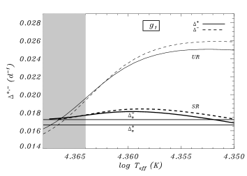
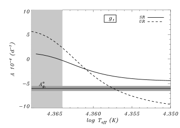
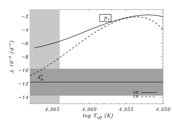
As expected, such variations principally affect the low-order ${\rm g}_{1}$ and ${\rm p}_{1}$ (see Fig. 7 for a comparison between the rotational kernels of UR, SR-${d_{\rm ov}}=0.28$, and SR-${d_{\rm ov}}=0.24$ models). In Fig. 8, the results for the asymmetries given in Fig. 6 (right column), which were computed with an overshooting parameter of ${d_{\rm ov}}=0.28$, are compared with those obtained from SR models computed with ${d_{\rm ov}}=0.24$. The best model found for this overshooting parameter value is SR2 (see Tables 2 and 3). In particular, a variation in ${d_{\rm ov}}$ of 0.04 results in differences in the asymmetry of the order of those found between UR and SR (${d_{\rm ov}}=0.28$) models, i.e. a few $10^{-4}\,{\rm d}^{-1}$ for ${\rm g}_{1}$ and ${\rm p}_{1}$, and about $10^{-4}\,{\rm d}^{-1}$, which represents almost one order of magnitude smaller than the difference between the results yield by the UR and SR (${d_{\rm ov}}=0.28$) models. Moreover, in the case of ${\rm p}_{1}$, the SR (${d_{\rm ov}}=0.24$) models fit the observed asymmetry in the limits of the observational uncertainties.

Figure 7: First-order rotational splitting kernel, from top to bottom, for the ${\rm g}_{1}$, ${\rm p}_{1}$, and ${\rm p}_{2}$ modes for the selected uniformly-rotating models (UR, dashed line) and differentially-rotating models (SR). For the latter models, two ${d_{\rm ov}}$ values are considered: 0.28 (continuous line) and 0.24 (dot-dashed line). Note that the position of the zeros and maxima for UR models is slightly shifted with respect to those of the SR models. This can be explained by small differences in the radii of both models, which, as expected, principally affects to the ${\rm g}_{1}$ and ${\rm p}_{1}$ split modes.

Figure 8: Comparison of the splitting asymmetries shown in Fig. 5 (for models with ${d_{\rm ov}}=0.28$), with those given by the models computed with ${d_{\rm ov}}=0.24$ (dot-dashed line). The additional vertical shaded band represents the range of ${T_{\mathrm{eff}}}$ defined by the models SR1, SR2, and UR1.

Furthermore, recent theoretical studies (Andrade, Suárez & Goupil 2008, work in progress), seem to indicate that even rough variations of the rotation profile may modify the asymmetries of the split modes. This modification can be as important as to change the sign of the asymmetries. According to this, the frequencies around ${\rm p}_{2}$ cannot be discarded as belonging to a rotationally split mode. However, if confirmed, the presence of such different asymmetries in the oscillation spectrum is very interesting, since they may significantly constrain the models providing information about the structure and rotation profile in the zones where they have more amplitude.

6 Conclusions

An asteroseismic analysis of the $\beta$ Cephei star $\nu$ Eridani  is presented, with focus on the study of the internal rotation profile. To this aim, a new method is presented based on the analysis of rotational splittings and their asymmetries. Some of the most updated asteroseismic modelling techniques are used, in particular, analysis of mode stability and improved descriptions for rotation effects. Regarding the latter, the so-called pseudo-rotating models are used, which consider radial differential rotation profiles (shellullar rotation) in both the evolutionary models and adiabatic oscillations computations. This represents an important qualitative step with respect to previous theoretical works.

The present work is divided into two parts. In the first part, a comparison of the different numerical packages (Liège, Warsaw-New Jersey, and Granada packages) was performed (the latter has been used in the present work). This comparison was performed using a mass-metallicity relation of the models fitting two of the observed frequencies. In that case, important differences in mass, up to $0.25\,{\mathrm{M}_{\odot}}$ between Liège models and ours, were found. Interestingly, differences between ASTA04’s models and ours can be explained by the different treatments of the overshooting implemented in the evolutionary codes. ASTA04’s models only take into account density variations in the overshooted region, which slightly affects the temperature gradient. On the other hand, our models were constructed considering an additional restriction by imposing that the real temperature gradient must equal the adiabatic gradient. Physically, this implies that, either the heat is transported efficiently outwards from the stellar core through convective movements due to the overshooting (the latter case), or purely by radiation (ASTA04’s treatment). This constitutes a very interesting challenge for asteroseismology, since the oscillation modes (low-order g and p modes) are sensitive to the physical description of the $\mu$ gradient zone.

Then, the previous exercise is extended to four frequencies with mode excitation included. In that case, models were also constrained to match the fundamental radial mode and three $m=0$ splitting components. Non-standard models built with a significant decrease of the initial hydrogen abundance, $X_{\rm i}=0.50$, were necessary to match and excite the modes. This provided models similar, but not identical, to those found by ASTA04 using a solar iron relative abundance, and the same initial hydrogen abundance. The remaining differences between ASTA04’s models and ours indicate that, for this level of the model accuracy, the present modelling still depend on the core overshooting. This parameter may change the physical conditions beyond the convective core. In that region, other physical processes take place, such as the mixing of chemical elements due to rotation. In particular, balance between rotationally induced turbulence and meridional circulation generates mixing of chemicals and redistribution of angular momentum (Zahn, 1992). This affects the rotation profile and the evolution of the star.

Secondly, the method here presented studies the asymmetries of the split modes in order to refine the modelling, and more importantly, provide information about the rotation profile of the star. To do so, pseudo-rotating models were built using the physical parameters provided in the first part of the work. Models with masses around $7.13\,{\mathrm{M}_{\odot}}$, and ages around 14.9 Myr, were found to fit better 10 of the 14 observed frequencies, which were identified as the fundamental radial mode and the three $\ell=1$ triplets ${\rm g}_{1}$, ${\rm p}_{1}$, and ${\rm p}_{2}$. For these modes, a comparison between the observed and predicted splittings and their asymmetries was performed. Two type of rotation profiles were considered: uniform rotation and shellular rotation profiles. Differences between predictions and observations were found to be of the order of $5\times 10^{-3}$ and $10^{-4}\,{\rm d}^{-1}$, for the rotational splittings and their asymmetries, respectively. For this last mode, none of the selected models reproduce neither the splittings, generally larger than the observed ones, nor the asymmetries, whose predictions have the opposite sign than the observed values. Although this result might indicate that the frequencies around ${\rm p}_{2},m=0$ mode do not belong to this rotationally-split mode, other possibilities cannot be discarded. In fact, a wrong physical description of the rotation profile may be responsible for a so peculiar result, particularly in the outer regions of the star. This result is very important because, up to now, none of the physical phenomena in which rotation plays a role predict variations of the rotation profile in that region. Furthermore, it is shown that asymmetries are quite dependent on the overshooting of the convective core. Therefore, the method here presented is suitable for testing the theories describing the angular momentum redistribution and chemical mixing due to rotationally-induced turbulence.

In general, the seismic models which include a description for shellular rotation yield slightly better results as compared with those given by uniformly-rotating models. Even so, further improvements are necessary in order to better constrain the modelling of $\nu$ Eridani. In particular, efforts should be focused in searching a better description of the rotation profile, for which a detailed study of asymmetries is required (work in progress). This may be enhanced by analysing other $\beta$ Cephei stars with larger rotational velocities, so that splittings and asymmetries are not of the same order than the frequency uncertainties.

References

- Aerts et al. (2004) Aerts, C., De Cat, P., Handler, G., et al. 2004, MNRAS, 347, 463
- Alexander & Ferguson (1994) Alexander, D. R. & Ferguson, J. W. 1994, ApJ, 437, 879
- Ausseloos et al. (2004) Ausseloos, M., Scuflaire, R., Thoul, A., & Aerts, C. 2004, MNRAS, 355, 352 (ASTA04)
- Baglin et al. (2002) Baglin A., Auvergne M., Barge P., Buey J.-T., Catala C., Michel E., Weiss W., COROT Team, 2002, in Battrick B., Favata F., Roxburgh I. W., Galadi D., eds, ASP Conf. Ser. Vol. 259, Radial and Nonradial Pulsations as Probes of Stellar Physics. Astron. Soc. Pac., San Francisco, p. 17
- Böhm-Vitense (1958) Böhm-Vitense E., 1958, Zeitschrift für Astrophysics, 46, 108
- Boury et al. (1975) Boury, A. and Gabriel, M. and Noels, A. and Scuflaire, R. and Ledoux, P. 1975, A&A, 41, 279
- Christensen-Dalsgaard & Daeppen (1992) Christensen-Dalsgaard, J. & Daeppen, W. 1992, A&A Rev., 4, 267
- Clayton (1968) Clayton, D. D. 1968, Principles of stellar evolution and nucleosynthesis (New York: McGraw-Hill, 1968)
- De Ridder et al. (2004) De Ridder, J., Telting, J. H., Balona, L. A., et al. 2004, MNRAS, 351, 324
- Dupret et al. (2002) Dupret, M.-A., De Ridder, J., Neuforge, C., Aerts, C., & Scuflaire, R. 2002, A&A, 385, 563
- Dziembowski & Jerzykiewicz (2003) Dziembowski, W. A. & Jerzykiewicz, M. 2003, in Astronomical Society of the Pacific Conference Series, 319
- Dziembowski & Pamiatnykh (1993) Dziembowski, W. A. & Pamiatnykh, A. A. 1993, MNRAS, 262, 204
- Eggleton et al. (1973) Eggleton, P. P., Faulkner, J., & Flannery, B. P. 1973, A&A, 23, 325
- Gautschy & Saio (1993) Gautschy, A. & Saio, H. 1993, MNRAS, 262, 213
- Grevesse & Noels (1996) Grevesse, N. & Noels, A. 1996, in Holt, S. S. and Sonneborn, G. eds, Vol. 99, Astron. Soc. Pac. Conference Series, 117
- Handler et al. (2004) Handler, G., Shobbrook, R. R., Jerzykiewicz, M., et al. 2004, MNRAS, 347, 454
- Iglesias & Rogers (1996) Iglesias, C. A. & Rogers, F. J. 1996, ApJ, 464, 943
- Jerzykiewicz, et al. (2005) Jerzykiewicz, M., Handler, G. & Shobbrook, R. R., et al. 2005, MNRAS, 360, 619
- Kippenhahn & Weigert (1990) Kippenhahn, R. & Weigert, A. 1990, ”Stellar structure and evolution”, Astronomy and Astrophysics library (Springer-Verlag)
- Kurucz (1993) Kurucz, R. 1993, ATLAS9 Stellar Atmosphere Programs and 2 km/s grid. Kurucz CD-ROM No. 13. Cambridge, Mass.: Smithsonian Astrophysical Observatory, 1993., 13
- Maeder & Meynet (2004) Maeder, A. & Meynet, G. 2004, in Maeder, A. and Eenens, P. eds, IAU Symposium, Vol. 215, Evolution of Massive Stars with Rotation and Mass Loss. Astron. Soc. Pac., San Franciscop. 500
- Michel et al. (1999) Michel, E. and Hernández, M. M. and Houdek, G. and Goupil, M. J. and Lebreton, Y. and Hernández, F. P. and Baglin, A. and Belmonte, J. A. and Soufi, F. 1999, A&A, 342, 153
- Morel (1997) Morel, P. 1997, A&AS, 124, 597
- Morel et al. (2006) Morel, T. and Butler, K. and Aerts, C. and Neiner, C. and Briquet, M. 2006, A&A, 457, 651
- Moya et al. (2004) Moya, A. and Garrido, R. and Dupret, M. A. 2004, A&A, 414, 1081
- Moya et al. (2007) Moya, A. and Garrido, R. 2008, Ap&SS, in press.
- Moya et al. (2008) Moya, A. and Christensen-Dalsgaard, J. and Charpinet, S. and Lebreton, Y. and Miglio, A. and Montalban, J. and Monteiro, M. J. P. F. G. and Provost, J. and Roxburgh, I. W. and Scuflaire, R. and Suárez, J. C. and Suran, M. 2008, Ap&SS, in press.
- Pamyatnykh (1975) Pamiatnykh A. A., 1975, in Sherwood, V. E., Plaut, L. eds, IAU Symp. 67. Variable Stars and Stellar Evolution. Dordrecht, Reidel Publishing, pp. 247
- Pamyatnykh et al. (2004) Pamyatnykh, A. A., Handler, G., & Dziembowski, W. A. 2004, MNRAS, 350, 1022
- Pérez Hernández et al. (1999) Pérez Hernández, F. and Claret, A. and Hernández, M. M. and Michel, E. 1999, A&A, 346, 586
- Schnerr et al. (2006) Schnerr, R. S. and Verdugo, E. and Henrichs, H. F. and Neiner, C. 2006, A&A, 452, 969
- Scuflaire et al. (2007) Scuflaire, R. and Théado, S. and Montalbán, J. and Miglio, A. and Bourge, P.-O. and Godart, M. and Thoul, A. and Noels, A. 2007, (Ap&SSin press), arXiv:0712.3471
- Smith, M. A. (1983) Smith, M. A. 1983, ApJ, 265, 338
- Suárez (2002) Suárez, J. C. 2002, Ph.D. Thesis, ISBN 84-689-3851-3, ID 02/PA07/7178
- Suárez et al. (2006) Suárez, J. C., Goupil, M. J., & Morel, P. 2006, A&A, 449, 673
- Suárez et al. (2007) Suárez, J. C. and Goupil, M. J. 2008, Ap&SS, in press
- Suárez et al. (2007) Suárez, J. C. and Michel, E. and Houdek, G. and Pérez Hernández, F. and Lebreton, Y. 2007, MNRAS, 379, 201
- Tran Minh & Léon (1995) Tran Minh, F. & L on, L. 1995, in Roxburg, I. W., Maxnou, J. L., eds., Physical Processes in Astrophysics. Springer Verlag, Berlin., 219
- Unno et al. (1989) Unno, W., Osaki, Y., Ando, H., Saio, H., & Shibahashi, H. 1989, Nonradial oscillations of stars (Nonradial oscillations of stars, Tokyo: University of Tokyo Press, 1989, 2nd ed.)
- van Hoof, A. (1961) van Hoof, A. 1961, Zeitschrift fur Astrophysik, 53, 106
- Dziembowski & Pamyatnykh (2008) Dziembowski, W. A. and Pamyatnykh, A. A. 2008, MNRAS, 385, 2061
- Zahn (1992) Zahn J.-P., 1992, A&A, 265, 115