Abstract

We calculate the one-photon loop radiative corrections to virtual pion Compton scattering $\pi^{-}\gamma^{*}\to\pi^{-}\gamma$, that subprocess which determines in the one-photon exchange approximation the pion-nucleus bremsstrahlung reaction $\pi^{-}Z\to\pi^{-}Z\gamma$. Ultraviolet and infrared divergencies of the loop integrals are both treated by dimensional regularization. Analytical expressions for the ${\cal O}(\alpha)$ corrections to the virtual Compton scattering amplitudes, $A(s,u,Q)$ and $B(s,u,Q)$, are derived with their full dependence on the (small) photon virtuality $Q$ from 9 classes of contributing one-loop diagrams. Infrared finiteness of these virtual radiative corrections is achieved (in the standard way) by including soft photon radiation below an energy cut-off $\lambda$. In the region of low $\pi^{-}\gamma$ center-of-mass energies, where the pion-nucleus bremsstrahlung process is used to extract the pion electric and magnetic polarizabilities, we find radiative corrections up to about $-3\%$ for $\lambda=5\,$MeV. Furthermore, we extend our calculation of the radiative corrections to virtual pion Compton scattering $\pi^{-}\gamma^{*}\to\pi^{-}\gamma$ by including the leading pion structure effect in form of the polarizability difference $\alpha_{\pi}-\beta_{\pi}$. Our analytical results are particularly relevant for analyzing the data of the COMPASS experiment at CERN which aims at measuring the pion electric and magnetic polarizabilities with high statistics using the Primakoff effect.

PACS: 12.20.-m, 12.20.Ds, 13.40.Ks, 14.70.Bh

1 Introduction and summary

At present there is much interest in a precise experimental determination of the pion electric and magnetic polarizabilities, $\alpha_{\pi}$ and $\beta_{\pi}$. Within the framework of current algebra [1] it has been shown (long ago) that the polarizability difference $\alpha_{\pi}-\beta_{\pi}$ of the charged pion is directly related to the axial-vector-to-vector form factor ratio $h_{A}/h_{V}\simeq 0.44$ measured in the radiative pion decay $\pi^{+}\to e^{+}\nu_{e}\gamma$ [2]. At leading (nontrivial) order the result of chiral perturbation theory [3], $\alpha_{\pi}-\beta_{\pi}=\alpha(\bar{l}_{6}-\bar{l}_{5})/(24\pi^{2}f_{\pi}^{2}m_{\pi})$, is of course the same after identifying the low-energy constant as $\bar{l}_{6}-\bar{l}_{5}=6h_{A}/h_{V}$. Recently, the systematic corrections to this current algebra result have been worked out in refs.[4, 5] by performing a full two-loop calculation of (real) pion Compton scattering in chiral perturbation theory. The outcome of that extensive analysis is that altogether the higher order corrections are rather small and the value $\alpha_{\pi}-\beta_{\pi}=(5.7\pm 1.0)\cdot 10^{-4}\,$fm³ [5] for the pion polarizability difference stands now as a firm prediction of the (chiral-invariant) theory. The non-vanishing value $\alpha_{\pi}+\beta_{\pi}=(0.16\pm 0.1)\cdot 10^{-4}\,$fm³ [5] for the pion polarizability sum (obtained also at two-loop order) is presumably much too small to cause an observable effect in low-energy pion Compton scattering.

However, the chiral prediction $\alpha_{\pi}-\beta_{\pi}=(5.7\pm 1.0)\cdot 10^{-4}\,$fm³ is in conflict with the existing experimental determinations of $\alpha_{\pi}-\beta_{\pi}=(15.6\pm 7.8)\cdot 10^{-4}\,$fm³ from Serpukhov [6] and $\alpha_{\pi}-\beta_{\pi}=(11.6\pm 3.4)\cdot 10^{-4}\,$fm³ from Mainz [7], which amount to values more than twice as large. Certainly, these existing experimental determinations of $\alpha_{\pi}-\beta_{\pi}$ raise doubts about their correctness since they violate the chiral low-energy theorem notably by a factor 2.

In that contradictory situation it is promising that the ongoing COMPASS [8] experiment at CERN aims at measuring the pion polarizabilities with high statistics using the Primakoff effect. The scattering of high-energy negative pions in the Coulomb field of a heavy nucleus (of charge $Z$) gives access to cross sections for $\pi^{-}\gamma$ reactions through the equivalent photons method [9]. In practice, one preferentially analyzes the spectrum of bremsstrahlung photons produced in the reaction $\pi^{-}Z\to\pi^{-}Z\gamma$ in the so-called Coulomb peak. This kinematical regime is characterized by very small momentum transfers to the nuclear target such that virtual pion Compton scattering $\pi^{-}\gamma^{*}\to\pi^{-}\gamma$ occurs as the dominant subprocess (in the one-photon exchange approximation). The deviations of the measured spectra (at low $\pi^{-}\gamma$ center-of-mass energies) from those of a point-like pion are then attributed to the pion structure as represented by its electric and magnetic polarizability [6] (taking often $\alpha_{\pi}+\beta_{\pi}=0$ as a constraint). It should be stressed here that the systematic treatment of virtual pion Compton scattering $\pi^{-}\gamma^{*}\to\pi^{-}\gamma$ in chiral perturbation theory yields at the same order as the polarizability difference $\alpha_{\pi}-\beta_{\pi}$ a further pion-structure effect in form of a unique pion-loop correction [10, 11] (interpretable as photon scattering off the “pion-cloud around the pion”). In the case of real pion Compton scattering $\pi^{-}\gamma\to\pi^{-}\gamma$ this loop correction compensates partly the effects from the pion polarizability difference [12]. A minimal requirement for improving future analyses of pion-nucleus bremsstrahlung $\pi^{-}Z\to\pi^{-}Z\gamma$ is therefore to include the loop correction predicted by chiral perturbation theory. The relevant analytical formulas for doing this have been written down in the appendix of ref.[11].

At the required level of accuracy it is also necessary to include higher order electromagnetic corrections to the pion-nucleus bremsstrahlung reaction $\pi^{-}Z\to\pi^{-}Z\gamma$. Such radiative corrections have been considered some time ago in the works of Akhundov et al. [13] and they have been implemented into the numerical program called RCFORGV. Unfortunately, no accessible sources to the underlying analytical expressions for the photon-loop amplitudes (which are necessary for an independent implementation into new data analyses) have been given by these authors. The purpose of the present work is to fill this gap. We will re-evaluate the one-photon loop radiative corrections to virtual pion Compton scattering $\pi^{-}\gamma^{*}\to\pi^{-}\gamma$ and present for each class of diagrams the corresponding analytical expressions. The calculation gets considerably simplified by considering the T-matrix of $\pi^{-}\gamma^{*}\to\pi^{-}\gamma$ in the laboratory frame and exploiting the circumstance that the time-like polarization vector $(1,\vec{0}\,)$ of the virtual photon is orthogonal to the space-like polarization vector $(0,\vec{\epsilon}\,)$ of the real bremsstrahlung photon. Incorporating furthermore crossing-symmetry, one finds that only two dimensionless amplitudes, $A(s,u,Q)$ and $B(s,u,Q)$, depending on three dimensionless Lorentz-invariant kinematical variables, need to be specified.

Our paper is organized as follows. In section 2, we review the cross section for pion-nucleus bremsstrahlung (in the one-photon exchange approximation) and define the T-matrix of virtual pion Compton scattering $\pi^{-}\gamma^{*}\to\pi^{-}\gamma$ in the laboratory frame together with the tree-level Born contributions. Section 3 is devoted to the calculation of the one-photon loop radiative corrections. We present analytical expressions for the amplitudes $A(s,u,Q)$ and $B(s,u,Q)$ of order $\alpha$ as they emerge from 9 classes of one-photon loop diagrams. Dimensional regularization is used to treat both ultraviolet and infrared divergencies of the loop integrals. While the ultraviolet divergencies drop out in the renormalizable scalar quantum electrodynamics at work, the infrared divergencies get removed (in the standard way) by including soft photon radiation below an energy cut-off $\lambda$. We evaluate in section 4 the resulting finite (real) radiative correction factor $\delta_{\rm real}^{\rm(cm)}$ with a small energy cut-off $\lambda$ introduced in the $\pi^{-}\gamma$ center-of-mass frame. Numerical results are presented for this part of the radiative corrections in the region of low $\pi^{-}\gamma$ invariant masses, where pion-nucleus bremsstrahlung is used to extract the pion polarizabilities. The detailed evaluation of the finite (virtual) radiative correction factor is not possible at this stage, since it requires specification and implementation of the actual experimental conditions (such as pion beam energy, constraints on the detectable energy and angular ranges, etc.). In section 5, we go beyond the works of Akhundov et al. [13] and extend the calculation of the radiative corrections to virtual pion Compton scattering $\pi^{-}\gamma^{*}\to\pi^{-}\gamma$ by including the leading pion structure effect (at low energies) in form of the polarizability difference $\alpha_{\pi}-\beta_{\pi}$. In an effective field theory approach this feature can be elegantly handled by a suitable (gauge-invariant) two-photon contact-vertex. In the appendix, we study some two-photon exchange processes specific to scalar quantum electrodynamics which turn out to be negligibly small.

Our analytical results for the radiative corrections to virtual pion Compton scattering can be utilized for analyzing the data of the COMPASS experiment at CERN which aims at measuring the pion polarizabilities via high-energy pion-nucleus bremsstrahlung $\pi^{-}Z\to\pi^{-}Z\gamma$.

2 Cross section for pion-nucleus bremsstrahlung

In order to keep this paper self-contained, we start with reviewing the cross section for pion-nucleus bremsstrahlung in the one-photon exchange approximation. Consider the process, $\pi^{-}(\vec{p}_{1})+Z_{\rm rest}\to\pi^{-}(\vec{p}_{2})+\gamma(\vec{k},\vec{\epsilon}\,)+Z_{\rm recoil}$, where a virtual photon transfers the (small) momentum $\vec{q}=\vec{p}_{2}+\vec{k}-\vec{p}_{1}$ from the nucleus (of charge $Z$) at rest to the (high-energetic) charged pion. The extremely small recoil energy $-q_{0}=\vec{q}\,^{2}/2M_{\rm nucl}\approx 0$ of the nucleus can be (safely) neglected. The corresponding fivefold differential cross section in the laboratory frame reads [14]:

$${d^{5}\sigma\over d\omega d\Omega_{\gamma}d\Omega_{\pi}}={Z^{2}\alpha^{3}\omega|\vec{p}_{2}|\over\pi^{2}|\vec{p}_{1}||\vec{q}\,|^{4}}\,H\,,$$ (1)

with $\alpha=1/137.036$ the fine-structure constant and $H$ a squared amplitude summed over the final state (real) photon polarizations $(\vec{\epsilon}\cdot\vec{k}=0)$:

$$H=|\tilde{A}\,\vec{p}_{1}\sin\theta_{1}|^{2}+|\tilde{B}\,\vec{p}_{2}\sin\theta_{2}|^{2}+2{\rm Re}(\tilde{A}\tilde{B}^{*})|\vec{p}_{1}||\vec{p}_{2}|\sin\theta_{1}\sin\theta_{2}\cos\phi\,.$$ (2)

It has been derived from a T-matrix for the virtual Compton scattering subprocess, $\pi^{-}\gamma^{*}_{0}\to\pi^{-}\gamma$, of the form $T_{\rm lab}=-8\pi\alpha(\tilde{A}\,\vec{\epsilon}\,^{*}\cdot\vec{p}_{1}+\tilde{B}\,\vec{\epsilon}\,^{*}\cdot\vec{p}_{2})$ with $\tilde{A}$ and $\tilde{B}$ two (in general complex) amplitudes. Since the electromagnetic interaction with the heavy nucleus involves only the charge density, the polarization four-vector of the virtual (Coulomb) photon has only a time-component: $(1,\vec{0}\,)$. The quantities $\theta_{1}$ and $\theta_{2}$ in eq.(2) are the angles between the momentum vectors $\vec{k}$ and $\vec{p}_{1}$ and between $\vec{k}$ and $\vec{p}_{2}$, respectively. Moreover, $\phi$ is the angle between the two planes spanned by $(\vec{k},\vec{p}_{1})$ and $(\vec{k},\vec{p}_{2})$. The photon energy is denoted by $\omega=|\vec{k}\,|=E_{1}-E_{2}$, where $E_{1}=\sqrt{|\vec{p}_{1}|^{2}+m_{\pi}^{2}}$ and $E_{2}=\sqrt{|\vec{p}_{2}|^{2}+m_{\pi}^{2}}$ are the initial and final pion energies in the laboratory frame.

Taking into account crossing-symmetry, the T-matrix for virtual pion Compton scattering, $\pi^{-}(\vec{p}_{1})+\gamma^{*}_{0}(\vec{q}\,)\to\pi^{-}(\vec{p}_{2})+\gamma(\vec{k},\vec{\epsilon}\,)$, in the laboratory frame can be further decomposed as:

$$T_{\rm lab}={8\pi\alpha\over m_{\pi}^{2}}\bigg{\{}\vec{\epsilon}^{\,\,*}\cdot\vec{p}_{1}\Big{[}E_{1}\,A(s,u,Q)+E_{2}\,B(s,u,Q)\Big{]}+\vec{\epsilon}^{\,\,*}\cdot\vec{p}_{2}\Big{[}E_{1}\,B(u,s,Q)+E_{2}\,A(u,s,Q)\Big{]}\bigg{\}}\,.$$ (3)

Here, we have introduced the (convenient) dimensionless Mandelstam variables: $s=(p_{2}+k)^{2}/m_{\pi}^{2}$, $u=(p_{1}-k)^{2}/m_{\pi}^{2}$, $t=(p_{1}-p_{2})^{2}/m_{\pi}^{2}$ and $Q=-q^{2}/m_{\pi}^{2}$ (given by Lorentz-squares of momentum four-vectors), which obey the constraint $s+t+u=2-Q$. In the physical region one has: $s>1$, $u<1$, $t<0$ and $Q>0$. The less obvious condition $u-1<0$ can be deduced by considering its left hand side in the $\pi^{-}\gamma$ center-of-mass frame. Due to the prefactor $8\pi\alpha/m_{\pi}^{2}$ in eq.(3) the two independent amplitudes $A(s,u,Q)$ and $B(s,u,Q)$ become also dimensionless quantities. The crossing symmetry of the T-matrix, which corresponds to an invariance under the transformation $(E_{1},\vec{p}_{1})\leftrightarrow(-E_{2},-\vec{p}_{2})$ and $s\leftrightarrow u$, is manifest according to the decomposition written in eq.(3).

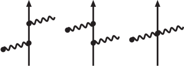
Figure 1: Tree diagrams of scalar QED for virtual pion Compton scattering. The virtual photon on the left hand side couples to heavy nucleus.

The advantage of working with dimensionless amplitudes and variables shows up already when calculating the Born terms for a point-like pion. The (three) tree diagrams of scalar quantum electrodynamics shown in Fig. 1 lead to the following extremely simple expressions:

$$A(s,u)^{(\rm tree)}=0\,,\qquad B(s,u)^{(\rm tree)}={2\over u-1}\,,$$ (4)

where we suppress from now on the dependence of $A(s,u,Q)$ and $B(s,u,Q)$ on the third variable $Q$. Note that the right diagram in Fig. 1 involving the two-photon contact-vertex of scalar QED vanishes, due to the orthogonality of the time-like virtual photon and the space-like real photon polarizations, $\epsilon_{0}=0$. The $s$-channel pole term (generated by the left diagram in Fig. 1) enters into the T-matrix through the (crossed) amplitude $B(u,s)^{(\rm tree)}=2/(s-1)$. The contributions of the pion polarizabilities (predominantly their difference $\alpha_{\pi}-\beta_{\pi}\simeq-2\beta_{\pi}$) to the amplitudes $A(s,u)$ and $B(s,u)$ can be found in eq.(27).

3 Evaluation of one-photon loop diagrams

In this section, we present analytical results for the one-photon loop radiative corrections of order $\alpha$ to the invariant amplitudes $A(s,u)$ and $B(s,u)$ of virtual pion Compton scattering. We use the method of dimensional regularization to treat both ultraviolet and infrared divergencies (where the latter are caused by the masslessness of the photon). The method consists in calculating loop integrals in $d$ spacetime dimensions and expanding the results around $d=4$. Divergent pieces of one-loop integrals generically show up in form of the composite constant:

$$\xi={1\over d-4}+{1\over 2}(\gamma_{E}-\ln 4\pi)+\ln{m_{\pi}\over\mu}\,,$$ (5)

containing a simple pole at $d=4$. In addition, $\gamma_{E}=0.5772\dots$ is the Euler-Mascheroni number and $\mu$ an arbitrary mass scale introduced in dimensional regularization in order to keep the mass dimension of the loop integrals independent of $d$. Ultraviolet (UV) and infrared (IR) divergencies are distinguished by the feature of whether the condition for convergence of the $d$-dimensional integral is $d<4$ or $d>4$. We discriminate them in the notation by putting appropriate subscripts, i.e. $\xi_{UV}$ and $\xi_{IR}$. The basic aspects of mass $(m_{\pi})$ and coupling constant $(e)$ renormalization in scalar QED have been discussed in section 2 of ref.[11].

The gauge condition $\epsilon_{0}=0$ eliminates those (five) loop diagrams where both the incoming virtual photon and the outgoing real photon are connected by the two-photon contact-vertex of scalar QED (in first or second order). One can also drop the diagrams with a tadpole-type self-energy insertion (the loop consisting of a single closed photon line) since it is set to zero in dimensional regularization. Thus we are left with 24 one-photon loop diagrams which we group into the (separately crossing-symmetric) classes I-IX, shown in Figs. 2-10. Due to an increasing number of internal pion propagators their evaluation rises in complexity. In order to simplify all calculations, we employ the Feynman gauge, where the photon propagator is directly proportional to the Minkowski metric tensor $g^{\mu\nu}$. We can now enumerate the analytical expressions for $A(s,u)$ and $B(s,u)$ as they emerge from the 9 classes of contributing one-photon loop diagrams.

Figure 2: One-photon loop diagrams of class I. The virtual photon comes in from the left.

Class I: For this class of diagrams the tree level amplitude in eq.(4) gets multiplied with the wavefunction renormalization factor of the pion:

$$B(s,u)^{(\rm I)}={2\alpha\over\pi(u-1)}\Big{(}\xi_{IR}-\xi_{UV}\Big{)}\,.$$ (6)

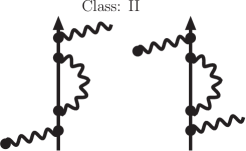
Figure 3: One-photon loop diagrams of class II.

Class II: These diagrams involve the once-subtracted (off-shell) self-energy of the pion:

$$B(s,u)^{(\rm II)}={\alpha\over\pi(u-1)}\bigg{[}-2\xi_{UV}+2-{u+1\over u}\ln(1-u)\bigg{]}\,.$$ (7)

Figure 4: One-photon loop diagrams of class III.

Class III: These diagrams generate a constant vertex correction factor:

$$B(s,u)^{(\rm III)}={\alpha\over\pi(u-1)}\bigg{[}3\xi_{UV}-{7\over 2}\bigg{]}\,.$$ (8)

Figure 5: One-photon loop diagrams of class IV.

Class IV: These diagrams generate a $u$-dependent vertex correction factor:

$$B(s,u)^{(\rm IV)}={\alpha\over\pi(u-1)}\bigg{[}3\xi_{UV}-3-{1\over 2u}+{u-1\over 2u^{2}}(3u+1)\ln(1-u)\bigg{]}\,.$$ (9)

Figure 6: One-photon loop diagrams of class V.

Class V: These diagrams generate also a $u$-dependent vertex correction factor:

$$B(s,u)^{(\rm V)}={\alpha\over 4\pi(u-1)}\bigg{[}-4\xi_{UV}+5+{1\over u}+{u^{2}+6u+1\over u^{2}}\ln(1-u)\bigg{]}\,.$$ (10)

Figure 7: One-photon loop diagrams of class VI.

Class VI: These diagrams generate a $u$- and $Q$-dependent vertex correction factor:

$$B(s,u)^{(\rm VI)} = {\alpha\over 4\pi(u-1)}\bigg{\{}-4\xi_{UV}+5+{1\over u}+{1-u^{2}\over u^{2}}\ln(1-u)$$ (11)

$$\qquad\qquad\quad-2(u+3+2Q)\int_{0}^{1}\!\!dx\!\int_{0}^{1}\!\!dy\,\,{1-y\over K(u,Q)}\,\bigg{\}}\,,$$

with the cubic polynomial $K(u,Q)=y+(1-u)x(1-y)+Qx(1-x)y$ in two Feynman parameters $x,y$. Note that in the physical region $u<1,Q>0$ the denominator $K(u,Q)>0$ is strictly positive and therefore the integral in eq.(11) is well-defined and can be performed easily numerically. Interestingly, for the classes I-VI considered up to here, the contributions to the amplitude $A(s,u)$ vanish identically in each case.

Figure 8: One-photon loop diagrams of class VII.

Class VII: These irreducible diagrams give:

$$A(s,u)^{(\rm VII)}={\alpha\over 4\pi(u-1)}\bigg{\{}{5-3u\over u}\ln(1-u)-2+{1\over u-1}\bigg{[}2{\rm Li}_{2}(u)-{\pi^{2}\over 3}\bigg{]}\bigg{\}}\,,$$ (12)

$$B(s,u)^{(\rm VII)}={\alpha\over 4\pi(u-1)}\bigg{\{}{1+u\over u}+{1-3u\over u^{2}}\ln(1-u)+{1\over u-1}\bigg{[}{\pi^{2}\over 3}-2{\rm Li}_{2}(u)\bigg{]}\bigg{\}}\,,$$ (13)

where Li${}_{2}(u)=\sum_{n=1}^{\infty}n^{-2}u^{n}=u\int_{1}^{\infty}dx[x(x-u)]^{-1}\ln x$ denotes the conventional dilogarithmic function.

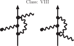
Figure 9: One-photon loop diagrams of class VIII.

Class VIII: These irreducible diagrams give:

$$A(s,u)^{(\rm VIII)}={\alpha\over 2\pi}\int_{0}^{1}\!\!dx\!\int_{0}^{1}\!\!dy\,\,{(1-y)(2-y+xy)\over K(s,Q)}\,,$$ (14)

$$B(s,u)^{(\rm VIII)}={\alpha\over 2\pi}\int_{0}^{1}\!\!dx\int_{0}^{1}\!\!dy\,\,{xy(y-1)\over K(u,Q)}\,.$$ (15)

The (singular) integral in eq.(14) involving $1/K(s,Q)$ requires a precise prescription for its (numerical) treatment. First, $s>1$ is given an infinitesimally positive imaginary part $s+i\,0^{+}$, which makes the integral complex-valued. In order to compute the only relevant real part of it, one performs analytically the Feynman parameter integral $\int_{0}^{1}dy$ and converts the occurring logarithm $\ln[x(1-s)]$ into $\ln[x(s-1)]$. The remaining integral $\int_{0}^{1}dx$ is free of poles and therefore unproblematic for a numerical treatment.

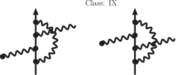
Figure 10: One-photon loop diagrams of class IX.

Class IX: These box diagrams are most tedious to evaluate and they give:

$$A(s,u)^{(\rm IX)} = {\alpha\over 2\pi}\Bigg{\{}{1\over u-1}-{u+1\over 2u(u-1)}\ln(1-u)+{1\over(u-1)^{2}}\bigg{[}{\pi^{2}\over 6}-{\rm Li}_{2}(u)\bigg{]}$$ (16)

$$+{1\over(Q+t)^{2}}\bigg{[}Q+t-4t\,L^{2}(-t)-4Q\,L^{2}(Q)+2Q\sqrt{4-t}\,L(-t)$$

$$-2Q\sqrt{4+Q}\,L(Q)\bigg{]}+\int_{0}^{1}\!\!dx\!\int_{0}^{1}\!\!dy\,\bigg{[}{(1-x)y(1-y)\over K(s,Q)}+(2t-4)xy$$

$$\times\int_{0}^{1}\!\!dz\,\bigg{(}{(1-x)(1+xy-y-xyz)\over G^{2}(s,t,Q)}+{x(1-xy)(1-z)\over G^{2}(u,t,Q)}\bigg{)}\bigg{]}\Bigg{\}}\,,$$

where we have introduced the frequently occurring logarithmic loop function:

$$L(x)={1\over\sqrt{x}}\ln{\sqrt{4+x}+\sqrt{x}\over 2}\,,$$ (17)

and the quartic polynomial $G(s,t,Q)=y+(1-s)x(1-y)z-tx(1-x)y(1-z)+Qx(1-x)yz$ in three Feynman parameters $x,y,z$. The other contribution reads:

$$B(s,u)^{(\rm IX)} = {\alpha\over 2\pi(u-1)}\Bigg{\{}{2u^{2}+u-1\over 2u^{2}}\ln(1-u)-{u+1\over 2u}+{1\over u-1}\bigg{(}{\rm Li}_{2}(u)-{\pi^{2}\over 6}\bigg{)}$$ (18)

$$+{2t-4\over\sqrt{t^{2}-4t}}\bigg{[}4\Big{(}\xi_{IR}+\ln(1-u)\Big{)}\sqrt{-t}\,L(-t)+{\rm Li}_{2}(w)-{\rm Li}_{2}(1-w)+{1\over 2}\ln^{2}w$$

$$-{1\over 2}\ln^{2}(1-w)+{\rm Li}_{2}(h_{-})-{\rm Li}_{2}(h_{+})-\sqrt{t^{2}-4t}\int_{0}^{1}\!\!dx\,{\ln[1+Qx(1-x)]\over 1-tx(1-x)}\bigg{]}\$$

$$+{u-1\over(Q+t)^{2}}\bigg{[}-Q-t+4t\,L^{2}(-t)+4Q\,L^{2}(Q)-2Q\sqrt{4-t}\,L(-t)$$

$$+2Q\sqrt{4+Q}\,L(Q)\bigg{]}+(u-1)\int_{0}^{1}\!\!dx\!\int_{0}^{1}\!\!dy\,\bigg{[}{(1-xy)(y-1)\over K(u,Q)}$$

$$+(2t-4)xy\int_{0}^{1}\!\!dz\,\bigg{(}{x(1-x)y(z-1)\over G^{2}(s,t,Q)}+{1-xy+x^{2}y+xz-x^{2}yz\over G^{2}(u,t,Q)}\bigg{)}\bigg{]}\Bigg{\}}\,,$$

with the auxiliary variables:

$$w={1\over 2}\Bigg{(}1-\sqrt{{-t\over 4-t}}\,\Bigg{)}\,,\qquad h_{\pm}={1\over 2}\Big{(}t\pm\sqrt{t^{2}-4t}\Big{)}\,,$$ (19)

depending on $t=2-s-u-Q$. In the physical region $u<1,t<0,Q>0$ the denominator polynomial $G(u,t,Q)>0$ is strictly positive and therefore the integrals involving $1/G^{2}(u,t,Q)$ are well-defined and suited for numerical evaluation. The (highly singular) integrals involving $1/G^{2}(s,t,Q)$ with $s>1$ (after the substitution $s\to s+i\,0^{+}$ which shifts the double-pole off the real integration contour) must however be treated partly analytically. The (solvable) integrals $\int_{0}^{1}dz$ over the third Feynman parameter $z$ appear in the following two versions:

$$\int_{0}^{1}\!\!dz\,{y\over G^{2}(s,t,Q)}={1\over[1-tx(1-x)]K(s,Q)}\,,$$ (20)

$$\int_{0}^{1}\!\!dz\,{x^{2}z\over G^{2}(s,t,Q)}={x\over N(s,Q+t)K(s,Q)}+{1\over N^{2}(s,Q+t)}\ln{K(s,Q)\over[1-tx(1-x)]y}\,,$$ (21)

giving rise to a new denominator polynomial $N(s,Q+t)=(s-1)(1-y)-(Q+t)(1-x)y>0$ which is strictly positive for $s>1$ and $t<-Q$. Although the latter condition $t<-Q$ does not hold in the entire physical region, it represents (fortunately) no restriction for the (experimentally selected) events in the Coulomb peak, where $Q<0.1$ (or even less). By analyzing the condition $t<-Q$ in the laboratory frame one deduces the inequality for the ratio of photon to pion beam energy, $\omega/E_{1}>[\sqrt{Q(4+Q)}-Q]/2\simeq\sqrt{Q}-Q/2$, which is indeed well satisfied for the experimentally selected events. In the next step, the terms in eqs.(20,21) with a factor $1/K(s,Q)$ are integrated once more analytically, $\int_{0}^{1}dy$, and for isolating the only relevant real parts the emerging logarithms are converted into logarithms of absolute values. The same conversion into real-valued logarithms is done with the term $\ln K(s,Q)$ in eq.(21), this time without solving the integral $\int_{0}^{1}dy$ analytically. The remaining single and double integrals are free of poles and thus suitable for a straightforward numerical evaluation. The same strategy for evaluating the occurring Feynman parameter integrals applies to the crossed amplitudes, $A(u,s)$ and $B(u,s)$, with the variables $s$ and $u$ interchanged. An alternative to the Feynman parameter representation of complicated loop functions in eqs.(11,14-18) is the (dispersive) spectral function representation based on the Kramers-Kronig dispersion relation (see section 3 in ref.[11]). However, at non-zero $Q$ the corresponding spectral functions (or imaginary parts) entering these principal value integrals turn out to be very cumbersome. If an expansion up to linear order in $Q$ suffices, one can do further steps in the analytical integration.

As a good check one verifies that the ultraviolet divergent terms proportional to $\xi_{UV}$ cancel in the total sum for $B(s,u)$. Interestingly, the contributions to the other amplitude $A(s,u)$ written in eqs.(12,14,16) are ultraviolet and infrared finite in each case.

4 Infrared finiteness

In the next step we have to consider the infrared divergent terms proportional to $\xi_{IR}$. Inspection of eqs.(6,18) reveals that they scale with the (tree level) Born amplitude written in eq.(4). As a consequence of that feature, the infrared divergent virtual (loop) corrections multiply the point-like differential cross section $d\sigma^{(\rm pt)}/d\omega d\Omega_{\gamma}d\Omega_{\pi}$ by a ($s\leftrightarrow u$ crossing-symmetric) factor:

$$\delta_{\rm virt}^{(\rm IR)}={2\alpha\over\pi}\Bigg{[}1+{2t-4\over\sqrt{4-t}}L(-t)\Bigg{]}\,\xi_{IR}\,.$$ (22)

The (unphysical) infrared divergence $\xi_{IR}$ gets canceled at the level of the (measurable) cross section by the contributions of soft photon bremsstrahlung. In its final effect, the (single) soft photon radiation multiplies the tree level cross section $d\sigma^{(\rm pt)}/d\omega d\Omega_{\gamma}d\Omega_{\pi}$ by a (universal) factor [11, 15]:

$$\delta_{\rm soft}=\alpha\,\mu^{4-d}\!\!\int\limits_{|\vec{l}\,|<\lambda}\!\!{d^{d-1}l\over(2\pi)^{d-2}\,l_{0}}\bigg{\{}{m_{\pi}^{2}(2-t)\over p_{1}\cdot l\,p_{2}\cdot l}-{m_{\pi}^{2}\over(p_{1}\cdot l)^{2}}-{m_{\pi}^{2}\over(p_{2}\cdot l)^{2}}\bigg{\}}\,,$$ (23)

which depends on a small energy cut-off $\lambda$. Working out this momentum space integral by the method of dimensional regularization (with $d>4$) one finds that the infrared divergent correction factor $\delta_{\rm virt}^{(\rm IR)}\sim\xi_{IR}$ in eq.(22) gets eliminated and the following finite radiative correction factor remains:

$$\delta^{\rm(cm)}_{\rm real} = {\alpha\over\pi}\Bigg{\{}\bigg{[}2+{4t-8\over\sqrt{4-t}}L(-t)\bigg{]}\ln{m_{\pi}\over 2\lambda}+{s+1\over 2(s-1)}\ln s$$ (24)

$$+{s+1+Q\over\sqrt{(s-1+Q)^{2}+4Q}}\ln{s+1+Q+\sqrt{(s-1+Q)^{2}+4Q}\over 2\sqrt{s}}$$

$$+(t-2)\int_{0}^{1}\!\!dx\,{s+1+Qx\over 2W[1-tx(1-x)]}\ln{s+1+Qx+W\over s+1+Qx-W}\Bigg{\}}\,,$$

with the abbreviation $W=\sqrt{(s+1+Qx)^{2}-4s+4stx(1-x)}$. We note that the terms beyond those proportional to $\ln(m_{\pi}/2\lambda)$ are specific for the evaluation of the soft photon correction factor $\delta_{\rm soft}$ in the $\pi^{-}\gamma^{*}$ center-of-mass frame with $\lambda$ an infrared cut-off therein. As an aside we mention that at $Q=0$ and in backward direction, $t=-(s-1)^{2}/s$, the integral in eq.(24) can be solved and one obtains the following handy formula:

$$\delta^{\rm(back)}_{\rm real} = {\alpha\over\pi(s^{2}-1)}\bigg{\{}2\Big{[}s^{2}-1-(s^{2}+1)\ln s\Big{]}\ln{m_{\pi}\over 2\lambda}$$ (25)

$$+(s+1)^{2}\ln s+(s^{2}+1)\Bigg{[}{1\over 2}\ln^{2}s+2{\rm Li}_{2}(1-s)\bigg{]}\bigg{\}}\,.$$

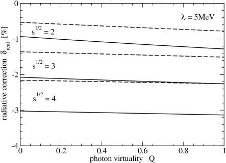
Figure 11: Radiative correction factor $\delta_{\rm real}^{(\rm cm)}$ for virtual pion Compton scattering $\pi^{-}\gamma^{*}\to\pi^{-}\gamma$ as a function of the photon virtuality $Qm_{\pi}^{2}$. The soft photon detection threshold has been set to $\lambda=5\,$MeV in the $\pi^{-}\gamma$ center-of-mass frame. Full and dashed lines correspond to backward and perpendicular scattering, respectively.

We can now present some numerical results for the radiative corrections to the pion-nucleus bremsstrahlung reaction $\pi^{-}Z\to\pi^{-}Z\gamma$. The radiative correction factor $\delta^{\rm(cm)}_{\rm real}$ due to soft photon emission vanishes for $t=Q=0$ at all $s>1$. The full curves in Fig. 11 show its values for three selected $\pi^{-}\gamma$ center-of-mass energies $\sqrt{s}m_{\pi}=(2,3,4)m_{\pi}$ as a function of $Q$ (the photon virtuality divided by $m_{\pi}^{2}$) choosing the extremal momentum transfer $t_{\rm min}$, where $-2s\,t_{\rm min}=(s-1)^{2}+Q(s+1)+(s-1)\sqrt{(s+1+Q)^{2}-4s}$ corresponds to the backward direction in the $\pi^{-}\gamma^{*}$ center-of-mass frame. The soft photon detection threshold has been set to $\lambda=5\,$MeV. One observes negative values up to $-3\%$ with a weak dependence on $Q$ (in particular in the region of the Coulomb peak $Q<0.1$). The three dashed lines in Fig. 11 show for comparison the case of perpendicular scattering with momentum transfer $t_{\perp}$ reduced to about one half of $t_{\rm min}$, where $-2s\,t_{\perp}=(s-1)^{2}+Q(s+1)$. At higher center-of-mass energies the excitation of the broad $\rho(770)$-resonance becomes prominent, $\sqrt{s_{\rho}}=m_{\rho}/m_{\pi}\simeq 5.5$. However, this kinematical region is not of interest for the extraction of the pion polarizabilities. The numbers in Fig. 11 should be considered only as indicative since there are yet the (finite) virtual radiative corrections due to the photon-loops. A comparison with the case of real pion Compton scattering [11] suggests that these will reduce the magnitude of the radiative corrections to pion-nucleus bremsstrahlung. At the present stage, a proper quantification of these (finite) virtual radiative corrections is not possible since that requires specification of the actual experimental conditions, such as pion beam energy, constraints on detectable energy and angular ranges, etc. However, their full implementation into the analysis of the COMPASS data is currently planned.

5 Inclusion of pion structure via polarizability difference

In the same way as Akhundov et al. [13], we have treated so far the pion as a structureless spin-0 boson in our calculation of the radiative corrections. Now we go beyond this approximation which is valid only near the $\pi^{-}\gamma$ threshold. The leading pion structure relevant for (virtual) Compton scattering is given by the difference of its electric and magnetic polarizability $\alpha_{\pi}-\beta_{\pi}$. In an effective field theory approach it is easily accounted for by a new two-photon contact-vertex proportional to the squared electromagnetic field strength tensor, $F_{\mu\nu}F^{\mu\nu}=2(\vec{B}^{2}-\vec{E}^{2})$. The S-matrix insertion following from this higher-order (gauge-invariant) effective $\pi\pi\gamma\gamma$-vertex reads:

$$8\pi i\beta_{\pi}m_{\pi}\Big{(}k_{1}\cdot k_{2}\,\epsilon_{1}\cdot\epsilon^{*}_{2}-\epsilon_{1}\cdot k_{2}\,\epsilon^{*}_{2}\cdot k_{1}\Big{)}\,,$$ (26)

where one photon $(k_{1},\epsilon_{1})$ is ingoing and the other one $(k_{2},\epsilon_{2})$ outgoing. At tree level (see left diagram in Fig. 12) the polarizability vertex eq.(26) gives in the kinematical situation of $\pi^{-}\gamma^{*}_{0}\to\pi^{-}\gamma$ rise to the (constant) contributions:

$$A(s,u)^{(\rm pola)}=-B(s,u)^{(\rm pola)}=-\,{\beta_{\pi}m_{\pi}^{3}\over\alpha}\,,$$ (27)

to the amplitudes $A(s,u)$ and $B(s,u)$ parameterizing the laboratory T-matrix $T_{\rm lab}$. In order to prevent any misunderstandings we stress that when writing (merely) $\beta_{\pi}m_{\pi}$ for the coupling strength in eq.(26), an electric and a magnetic pion polarizability, equal in magnitude and opposite in sign $\alpha_{\pi}=-\beta_{\pi}$, are always both included.

We reinterpret now the one-photon loop diagrams of section 3 in such a way that the two-photon contact-vertex represents one polarizability vertex proportional to $\beta_{\pi}m_{\pi}$. In order to distinguish it from the leading order contact-vertex $8\pi i\alpha\,\epsilon_{1}\cdot\epsilon^{*}_{2}$ of scalar QED we have symbolized it in Figs. 12-15 by an open square. Going through the classes I’- V’ and evaluating the loop diagrams with the S-matrix insertion from the polarizability vertex we find the following contributions to the amplitudes $A(s,u)$ and $B(s,u)$.

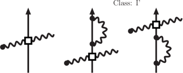
Figure 12: The open square symbolizes the electromagnetic interaction proportional to the (dominant) pion polarizability difference $\alpha_{\pi}-\beta_{\pi}$. Shown are the tree diagram and the diagrams of class I’ involving the pion wavefunction renormalization factor.

Class I’:

$$A(s,u)^{(\rm I^{\prime})}=-B(s,u)^{(\rm I)}={\beta_{\pi}m_{\pi}^{3}\over\pi}\Big{(}\xi_{UV}-\xi_{IR}\Big{)}\,.$$ (28)

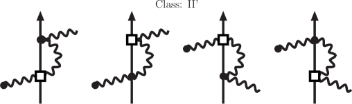
Figure 13: One-photon loop diagrams of class II’ including pion structure via its polarizability difference.

Class II’:

$$A(s,u)^{(\rm II^{\prime})}={\beta_{\pi}m_{\pi}^{3}\over 2\pi}\bigg{[}-2\xi_{UV}+2-{1\over 2s}-{1\over 2u}-{(s-1)^{2}\over 2s^{2}}\ln(1-s)-{(u-1)^{2}\over 2u^{2}}\ln(1-u)\bigg{]}\,,$$ (29)

$$B(s,u)^{(\rm II^{\prime})}={\beta_{\pi}m_{\pi}^{3}\over 2\pi}\bigg{[}2\xi_{UV}-2+{1\over u}+{(u-1)^{2}\over u^{2}}\ln(1-u)\bigg{]}\,.$$ (30)

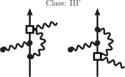
Figure 14: One-photon loop diagrams of class III’.

Class III’

$$A(s,u)^{(\rm III^{\prime})}={\beta_{\pi}m_{\pi}^{3}\over 2\pi}\bigg{\{}-\xi_{UV}+{1\over 4}+\int_{0}^{1}\!\!dx\!\int_{0}^{1}\!\!dy\,y\bigg{[}{(s-1)x(1-y)\over K(s,Q)}-\ln K(s,Q)\bigg{]}\bigg{\}}\,,$$ (31)

$$B(s,u)^{(\rm III^{\prime})}={\beta_{\pi}m_{\pi}^{3}\over 2\pi}\bigg{\{}\xi_{UV}-{1\over 4}+\int_{0}^{1}\!\!dx\!\int_{0}^{1}\!\!dy\,y\bigg{[}{(s-1)x(1-y)\over K(u,Q)}+\ln K(s,Q)\bigg{]}\bigg{\}}\,,$$ (32)

with the polynomial $K(u,Q)$ defined below eq.(11). The strategy to compute the integrals involving $1/K(s,Q)$ and $\ln K(s,Q)$ has been described in section 3.

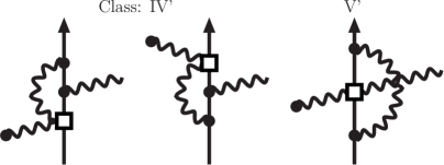
Figure 15: One-photon loop diagrams of classes IV’ and V’.

Class IV’:

$$A(s,u)^{(\rm IV^{\prime})} = {\beta_{\pi}m_{\pi}^{3}\over 2\pi}\bigg{\{}-\xi_{UV}+{3\over 2}-{u+1\over 2u}\ln(1-u)+{1\over u-1}\bigg{[}{\pi^{2}\over 6}-{\rm Li}_{2}(u)\bigg{]}$$ (33)

$$+{u-1-Q\over u-1}\bigg{[}{3u-1\over 2u^{2}}\ln(1-u)-{u+1\over 2u}+{1\over u-1}\bigg{(}{\rm Li}_{2}(u)-{\pi^{2}\over 6}\bigg{)}\bigg{]}\bigg{\}}\,,$$

$$B(s,u)^{(\rm IV^{\prime})} = {\beta_{\pi}m_{\pi}^{3}\over 2\pi}\bigg{\{}\xi_{UV}-{3\over 2}+{s+1\over 2s}\ln(1-s)+{1\over s-1}\bigg{[}{\rm Li}_{2}(s)-{\pi^{2}\over 6}\bigg{]}$$ (34)

$$+{s-1+Q\over u-1}\bigg{[}{3u-1\over 2u^{2}}\ln(1-u)-{u+1\over 2u}+{1\over u-1}\bigg{(}{\rm Li}_{2}(u)-{\pi^{2}\over 6}\bigg{)}\bigg{]}\bigg{\}}\,.$$

Class V’:

$$A(s,u)^{(\rm V^{\prime})} = -B(s,u)^{(\rm V^{\prime})}={\beta_{\pi}m_{\pi}^{3}\over 2\pi}\bigg{\{}\xi_{UV}-1-\sqrt{4-t}\,L(-t)+{2-t\over\sqrt{t^{2}-4t}}$$ (35)

$$\times\bigg{[}4\xi_{IR}\sqrt{-t}\,L(-t)+{\rm Li}_{2}(w)-{\rm Li}_{2}(1-w)+{1\over 2}\ln^{2}w-{1\over 2}\ln^{2}(1-w)\bigg{]}\bigg{\}}\,,$$

with the auxiliary variable $w$ defined in eq.(19). The contributions of the vertex type diagrams (classes III and IV in Figs. 4,5) vanish due to some special features of the polarizability vertex eq.(26).

At first count the ultraviolet divergent terms proportional to $\xi_{UV}$ do not drop out in the total sums for $A(s,u)$ and $B(s,u)$. They disappear however after interpreting the coupling constant in eq.(27) as a bare one and splitting it as $\beta_{\pi}^{(\rm bare)}=\beta_{\pi}(1-\alpha\,\xi_{UV}/2\pi)$ into the physical coupling constant $\beta_{\pi}$ and a counterterm piece. Note that the same renormalization procedure has rendered the radiative corrections to real pion Compton scattering ultraviolet finite [11]. The infrared divergent terms proportional to $\xi_{IR}$ showing up in eqs.(28,35) are again canceled by the soft photon bremsstrahlung contributions. As a result one has to multiply the partial differential cross section $d\sigma^{(\rm pol)}/d\omega d\Omega_{\gamma}d\Omega_{\pi}$ linear in $\beta_{\pi}$, which arises from the interference of the Born and polarizability terms in eqs.(4,27), with the radiative correction factor $\delta^{(\rm cm)}_{\rm real}$ written down in eq.(24). In the case of real pion Compton scattering it has been observed in ref.[11] that the inclusion the leading pion structure effect (via $\alpha_{\pi}-\beta_{\pi}\simeq-2\beta_{\pi}$) does not change the relative size and angular dependence of the radiative corrections. Due to the dominance of real over the virtual radiative corrections (for small enough infrared cut-off $\lambda$) one can expect that the same feature holds for the pion-nucleus bremsstrahlung reaction $\pi^{-}Z\to\pi^{-}Z\gamma$.

Appendix: Specific two-photon exchange contributions

For high nuclear charges $Z$ the one-photon exchange approximation is insufficient for analyzing experimental data of pion-nucleus bremsstrahlung $\pi^{-}Z\to\pi^{-}Z\gamma$. A non-perturbative treatment of the scattering of the charged particles in the strong nuclear Coulomb field is required in this case. Integrating the tree-level cross section $d\sigma^{(\rm pt)}/d\omega d\Omega_{\gamma}d\Omega_{\pi}$ of scalar QED over the angles $(\theta_{1},\theta_{2},\phi)$, and adapting the result of refs.[16, 17] obtained for electrons to pions, one may write the photon spectrum at high beam energies $E_{1}$ in the form:

$${d\sigma\over d\omega}^{(\rm pt)}={16Z^{2}\alpha^{3}E_{2}\over 3m_{\pi}^{2}E_{1}\omega}\bigg{\{}\ln{2E_{1}E_{2}\over m_{\pi}\omega}-{1\over 2}+\Psi_{\pi}(Z\alpha)\bigg{\}}\,,$$ (36)

with $\omega=E_{1}-E_{2}$ the photon laboratory energy. The function $\Psi_{\pi}(Z\alpha)$ represents the non-perturbative corrections beyond the one-photon exchange. For electrons this function has been calculated as $\Psi_{e}(Z\alpha)=-Z^{2}\alpha^{2}\sum_{n=1}^{\infty}[n(n^{2}+Z^{2}\alpha^{2})]^{-1}$ in refs.[16, 17]. In the case of a lead or a nickel target ($Z=82$ or $28$) the negative infinite series $\Psi_{e}(Z\alpha)$ amounts to $-0.3316$ or $-0.0484$, i.e. about a $-5\%$ or $-0.7\%$ correction compared to the leading logarithm plus constant in eq.(36). At this point it would be most important to clarify, whether these non-perturbative corrections are the same for pions and electrons or not.

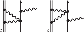
Figure 16: Two-photon exchange diagrams specific for the contact-vertex of scalar QED. The double-line symbolizes the heavy nucleus of charge $Z$.

As a supplement to the subject, we evaluate in this appendix those two-photon exchange contributions (of order $Z^{2}$ in the transition amplitude) which are specific to the two-photon contact-vertex of scalar QED. The pertinent one-loop diagrams are shown in Fig. 16. Additionally possible box and crossed box type diagrams, where one exchanged virtual photon and the emitted real photon are connected by the contact-vertex vanish as a consequence of the gauge condition $\epsilon_{0}=0$. For the evaluation of the (triangular) loop we use a non-relativistic (static) propagator $i/(l_{0}+i\,0^{+})$ for the intermediate heavy nucleus. By dividing out the factor $-eZ/|\vec{q}\,|^{2}$ we can translate the two-photon exchange processes into a correction to the T-matrix $T_{\rm lab}$ of virtual pion Compton scattering. Putting all pieces together we find from the photon-loop diagrams in Fig. 16 the following contribution:

$$T_{\rm lab}^{(2\gamma)}=(2\pi\alpha)^{2}Z{\sqrt{Q}\over m_{\pi}}\Bigg{(}{\vec{\epsilon}^{\,\,*}\cdot\vec{p}_{1}\over u-1}+{\vec{\epsilon}^{\,\,*}\cdot\vec{p}_{2}\over s-1}\Bigg{)}\,.$$ (37)

It has a structure very similar to the T-matrix in Born approximation (see eqs.(3,4)). Making this comparison explicitly, one deduces that the coupling terms $\vec{\epsilon}^{\,\,*}\cdot\vec{p}_{1,2}$ in eq.(37) carry the relative suppression factors $\pi\alpha Zm_{\pi}\sqrt{Q}/4E_{2,1}$, respectively. Although $\pi\alpha Z/4\simeq 0.47$ is already sizeable for a lead target ($Z=82$), the ratio $|\vec{q}\,|/E_{1,2}$ of (virtual photon) momentum transfer to beam or scattered pion energy reduces it by at least three orders of magnitude. We are considering here the typical kinematical situation, $E_{1,2}>50\,$GeV and $|\vec{q}\,|<50\,$MeV, where high-energy pion-nucleus bremsstrahlung $\pi^{-}Z\to\pi^{-}Z\gamma$ is used to extract the pion polarizabilities. In passing we note that the diagrams in Fig. 16 with the contact-vertex replaced by the polarizability vertex give rise to a T-matrix that differs from eq.(37) merely by an additional prefactor $\beta_{\pi}m_{\pi}^{3}Q/2\alpha\simeq-7\cdot 10^{-3}\,Q$ (using $\alpha_{\pi}=-\beta_{\pi}\simeq 3\cdot 10^{-4}\,$fm³). We can therefore conclude that the two-photon exchange mechanisms in Fig. 16, specific to the pseudo-scalar pion, are negligibly small.

References

- [1] M.V. Terentev, Sov. J. Nucl. Phys. 16, 87 (1973).
- [2] E. Frlez et al., Phys. Rev. Lett. 93, 181804 (2004); hep-ex/0606023.
- [3] J.F. Donoghue and B.R. Holstein, Phys. Rev. D40, 2378 (1989).
- [4] U. Bürgi, Phys. Lett. B377, 147 (1996); Nucl. Phys. B479, 392 (1996).
- [5] J. Gasser, M.A. Ivanov, and M.E. Sainio, Nucl. Phys. B745, 84 (2006); and refs. therein.
- [6] Y.M. Antipov et al., Phys. Lett. B121, 445 (1983); Z. Phys. C26, 495 (1985).
- [7] J. Ahrens et al., Eur. Phys. J. A23, 113 (2005).
- [8] COMPASS Collaboration: P. Abbon et al., hep-ex/0703049.
- [9] I.Y. Pomeranchuk and I.M. Shmushkevich, Nucl. Phys. 23, 452 (1961).
- [10] C. Unkmeir, S. Scherer, A.I. Lvov, and D. Drechsel, Phys. Rev. C61, 034002 (2000).
- [11] N. Kaiser and J.M. Friedrich, Nucl. Phys. A812, 186 (2008).
- [12] N. Kaiser and J.M. Friedrich, Eur. Phys. J. A36, 181 (2008).
-
[13]
A.A. Akhundov, D.Y. Bardin, and G.V. Mitselmakher,
Sov. J. Nucl. Phys. 37, 217 (1983);
A.A. Akhundov, D.Y. Bardin, G.V. Mitselmakher, and A.G. Olshevskii, Sov. J. Nucl. Phys. 42, 426 (1985);
A.A. Akhundov, S. Gerzon, S. Kananov, and M.A. Moinester, Z. Phys. C66, 279 (1995). - [14] C. Itzykson and J.B. Zuber, Quantum Field Theory, McGraw-Hill book company, 1980; chapter 5.2.4.
- [15] M. Vanderhaeghen et al., Phys. Rev. C62, 025501 (2000); and refs. therein.
-
[16]
H.A. Bethe and L.C. Maximon, Phys. Rev. 93,
768 (1954);
H. Olsen, Phys. Rev. 99, 1335 (1955). - [17] L.D. Landau and E.M. Lifschitz, Quantenelektrodynamik, Akademie-Verlag Berlin, 1986; section 96.