Computer Simulations of Pulsatile Human Blood Flow Through 3D-Models of the Human Aortic Arch, Vessels of Simple Geometry and a Bifurcated Artery: Investigation of Blood Viscosity and Turbulent Effects

Abstract

We report computational results of blood flow through a model of the human aortic arch and a vessel of actual diameter and length. On the top of the aortic arch the branching of the arteries are included: the subclavian and jugular. A realistic pulsatile flow is used in all simulations. Calculations for bifurcation type vessels are also carried out and presented. Different mathematical methods for numerical solution of the fluid dynamics equations have been considered. The non-Newtonian behaviour of the human blood is investigated together with turbulence effects. A detailed time-dependent mathematical convergence test has been carried out. The results of computer simulations of the blood flow in vessels of three different geometries are presented: for pressure, strain rate and velocity component distributions we found significant disagreements between our results obtained with realistic non-Newtonian treatment of human blood and the widely used method in the literature: a simple Newtonian approximation. A significant increase of the strain rate and, as a result, a wall shear stress distribution, is found in the region of the aortic arch. Turbulent effects are found to be important, particularly in the case of bifurcation vessels.

I Introduction

Cardiovascular diseases, such as ischemic heart disease, myocardial infarction, and stroke are leading causes of death in Western countries. All of these vascular diseases share a common element: atherosclerosis. They also share a common final event: the failure or destruction of the vascular wall structure 1-lee05 ; 2-dhein05 .

Atherosclerosis reduces arterial lumen size through plaque formation and arterial wall thickening and it occurs at specific arterial sites. This phenomenon is related to hemodynamics and to wall shear stress (WSS) distribution fung93 . From the physical point of view WSS is the tangential drag force produced by moving blood, and it is a mathematical function of the velocity gradient of blood near the endothelial surface landau . Arterial wall remodeling is regulated by WSS grotberg04 . For example, in response to high shear stress arteries enlarge.

Further, from the biomechanical point of view one can conclude, that the atherosclerotic plaques localize preferentially in the regions of low shear stresses, but not in regions of higher shear stresses. Furthermore, decreased shear stress induces intimal thickening in vessels which have adapted to high flow.

Final vascular events that induce fatal outcomes, such as acute coronary syndrome, are triggered by the sudden mechanical disruption of an arterial wall. Thus, we can conclude, that the final consequences of tragic fatal vascular diseases are strongly connected to mechanical events that occur on the vascular wall, and these, in turn, which are likely to be heavily influenced by alterations in blood flow and the characteristics of the blood itself.

Currently researchers in the field of biomechanics and biomedicine conduct laboratory investigations of human blood flow in different shape and size tubes, which are designed to be approximate models of human vessels and arteries, see for example 19 ; 2 . Some researchers also carry out intensive computer simulations of these bio-mechanical systems, see for example 362 ; 1991 ; 9 ; chn04 ; 8 ; morris2004 ; chn06 ; dur2007 ; pre08 ; renat08 ; renat08a .

Also, in some special laboratory works specific stents are incorporated in such artifical vessels (tubes). Stent implantation has been used to open diseased coronary blood vessels, allowing improved perfusion of the cardiac muscle. Used in combination with drug therapy, vascular repair and dilation techniques (angioplasty) the use of metallic stents has created a multibillion dollar industry. Stents are commonly used in many different blood vessels, but the primary site of deployment is in diseased coronary arteries.

Stents represent a very special case in the modeling research problems mentioned above 77 . Taking into account that stents have a very small size and rather complicated structure and shape, this situation makes it difficult to obtain precise measurements. Therefore high quality and precise computer simulations of blood flow through vessels with implanted stents would be most useful 77 . Work of this type is already underway and we would like to mention several pertinent studies 6a ; 3a ; 10a ; 11a .

Nevertheless, there are still many difficulties in obtaining precise realistic geometries for the required vessels. Human arteries, especially the aorta, have complicated spatial-geometric and characteristic configurations. For example, the aortic arch centerline does not lie on a plane and there are major branches at the top of the arch feeding the carotid arterial circulation. One of the main problems in the field of bio-medical blood flow simulation is to obtain precise geometrical-mathematical representations of different vessels. This information in turn needs to be included in the simulation programs.

However, in our opinion, as a first step of these investigations it would be useful to apply simpler 3D-geometry forms and models, but to take into account as much as possible the precise physical effects of blood movement such as the non-Newtonian characteristics of human blood, realistic pulsatile flow, and possible turbulent effects. Because of pulsatility the last one may be significant in contributing to the final results of this study.

In the current work we carried out real-time full-dimensional computer simulations of a realistic pulsatile human blood flow in actual size vessels, vessels with a bifurcation, and in a model of the aortic arch. We take into account different physical effects, such as turbulence and the non-Newtonian nature of human blood. The next section presents the mathematical methodology and the physical model used in this work. The general purpose commercial computational fluid dynamics program FLOW3D is used for its basic functionality, but we supplemented its capability by adding our routines to obtain the results presented in this work.

Sec. 3 presents results for three vessels of different geometries. The CGS unit system is used in all simulations, as well as for presentation of the results. Conclusions and discussion comparing our results to well respected studies is included in Sec. 4.

II Mathematical methodology and physical models

As we mentioned above, we undertook pulsatile human blood flow simulation experiments using different size and shape human vessel arteries. For each spatial configuration one needs to provide a specific approach for the numerical solution to the complicated second order partial differential equations of the fluid dynamics (FD). For example, for simple cylindrical vessels we used the cylindrical coordinate system: $\vec{r}={(r,\theta,\phi)}$. However, for the aortic arch or bifurcated vessels, where there is no cylindrical symmetry, we applied the Cartezian coordinate system: $\vec{r}={(x,y,z)}$. In the cases of the aortic arch and bifurcated vessels we used up to five blocks of matched Cartezian coordinate subsystems.

Below we present the FD equations in a general form, because, for each of the special cases, considered in this work and the chosen coordinate system, the partial differential equations of the fluid dynamics may look different, although we understand, that the general differential operator form of the equations is always unique.

II.1 Equations

The equations of motion for the fluid velocity components $(u,v,w)$ in the 3-coordinate system are the Navier-Stokes equations with specific additional terms included in the FLOW3D program:

$$\frac{\partial u}{\partial t}+\frac{1}{V_{F}}({uA_{x}\frac{\partial u}{\partial x}}+{vA_{y}R\frac{\partial u}{\partial y}}+{wA_{z}\frac{\partial u}{\partial z}})-\xi\frac{A_{y}v^{2}}{xV_{f}}=-\frac{1}{\rho}\frac{\partial p}{\partial x}+G_{x}+f_{x}-b_{x}-$$

$$\frac{R_{sor}}{\rho V_{f}}(u-u_{w}-\delta\cdot u_{s})$$ (1)

$$\frac{\partial v}{\partial t}+\frac{1}{V_{F}}({uA_{x}\frac{\partial v}{\partial x}}+{vA_{y}R\frac{\partial v}{\partial y}}+{wA_{z}\frac{\partial v}{\partial z}})+\xi\frac{A_{y}uv}{xV_{f}}=-\frac{R}{\rho}\frac{\partial p}{\partial y}+G_{y}+f_{y}-b_{y}-$$

$$\frac{R_{sor}}{\rho V_{f}}(v-v_{w}-\delta\cdot v_{s})$$ (2)

$$\frac{\partial w}{\partial t}+\frac{1}{V_{F}}({uA_{x}\frac{\partial w}{\partial x}}+{vA_{y}R\frac{\partial w}{\partial y}}+{wA_{z}\frac{\partial w}{\partial z}})=-\frac{1}{\rho}\frac{\partial p}{\partial z}+G_{z}+f_{z}-b_{z}-$$

$$\frac{R_{sor}}{\rho V_{f}}(w-w_{w}-\delta\cdot w_{s}).$$ (3)

Here, $(u,v,w)$ are the velocity components in coordinate directions $(x,y,z)$ respectively. For example, when Cartesian coordinates are used, $R=1$ and $\xi=0$, see FLOW3D manual flow3d . $A_{x}$ is the fractional area open to flow in the $x$ direction, analogously for $A_{y}$ and $A_{z}$. Next, $V_{F}$ is the fractional volume open to flow, $R$ and $\xi$ are coefficients which depend on the coordinate system: $(x,y,z)$ or $(r,\theta,z)$, $\rho$ is the fluid density, $R_{sor}$ is a mass source term. Finally, $(G_{x},G_{y},G_{z})$ are so called body accelerations flow3d , $(f_{x},f_{y},f_{z})$ are viscous accelerations, $(b_{x},b_{y},b_{z})$ are the flow losses in porous media or across porous baffle plates, and the final term accounts for the injection of mass at a source represented by a geometry component. Mathematical expressions for the viscous accelerations $(f_{x},f_{y},f_{z})$ are presented in the Appendix.

The term $U_{w}=(u_{w},v_{w},w_{w})$ in equation (1) is the velocity of the source component, which will generally be non-zero for a mass source at a General Moving Object (GMO) flow3d . The term $U_{s}=(u_{s},v_{s},w_{s})$ is the velocity of the fluid at the surface of the source relative to the source itself. It is computed in each control volume as

$$\vec{U}_{s}=\frac{1}{\rho_{s}}\frac{d(Q\vec{n})}{dA}$$ (4)

where $dQ$ is the mass flow rate, $\rho_{s}$ fluid source density, $dA$ the area of the source surface in the cell and $\vec{n}$ the outward normal to the surface. The source is of the stagnation pressure type when in equations. (1-3) $\delta=0.0$. Next, $\delta=1.0$ corresponds to the source of the static pressure type.

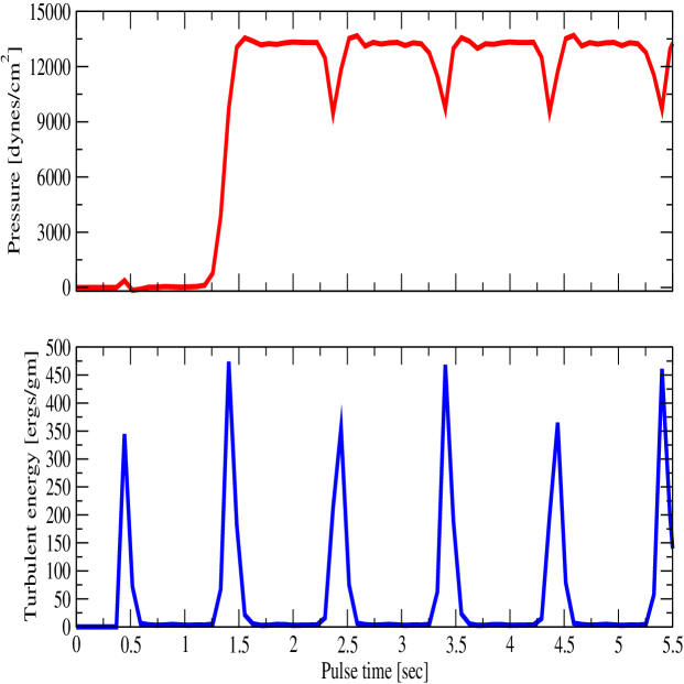
Figure 3: Time-dependent results for pressure and the turbulent energy in the middle point of the cylinder. The non-Newtonian viscosity.

As we already mentioned, in all simulations we considered the blood flow as a pulsatile flow. The final result for the inflow waveform has been taken from figure 3 of work greece2007 . The values of the velocity waveform, which were used in our simulations, are shown in Table 1 depending on pulse time. The pulse was applied for 5.5 cycle times in our work.

These velocity values are used as time-dependent inflow initial boundary conditions. These numbers are included directly in the FLOW3D program.

Next, the general mass continuity equation, which is solved within the FLOW3D program has the following general form:

$$V_{f}\frac{\partial\rho}{\partial t}+\frac{\partial}{\partial x}(\rho uA_{x})+R\frac{\partial}{\partial y}(\rho vA_{y})+\frac{\partial}{\partial z}(\rho wA_{z})+\xi\frac{\rho uA_{x}}{x}=R_{dif}+R_{sor},$$ (5)

$R_{dif}$ is a turbulent diffusion term, and $R_{sor}$ is a mass source. The turbulent diffusion term is

$$R_{dif}=\frac{\partial}{\partial x}(v_{p}A_{x}\frac{\partial\rho}{\partial x})+R\frac{\partial}{\partial y}(v_{p}A_{y}R\frac{\partial\rho}{\partial y})+\frac{\partial}{\partial z}(v_{p}A_{z}\frac{\partial\rho}{\partial z})+\xi\frac{\rho v_{p}A_{x}}{x},$$ (6)

where the coefficient $v_{p}=C_{p}\mu/\rho$, $\mu$ is dynamic viscosity and $C_{p}$ is a constant. The $R_{sor}$ term is a density source term that can be used to model mass injections through porous obstacle surfaces.

Compressible flow problems require the solution of the full density transport equation In this work we treated blood as an incompressible fluid. For incompressible fluids, $\rho=constant$ and the equation (2) becomes the following:

$$\frac{\partial}{\partial x}(uA_{x})+\frac{\partial}{\partial y}(vA_{y})+\frac{\partial}{\partial z}(wA_{z})+\xi\frac{uA_{x}}{x}=\frac{R_{sor}}{\rho}.$$ (7)

It is assumed, that at a stagnation pressure source fluid enters the domain at zero velocity. As a result, pressure should be considered at the source to move the fluid away from the source. For example, such sources are designed to model fluid emerging at the end of a rocket or the simple deflating process of a balloon.

In general, stagnation pressure sources apply to cases when the momentum of the emerging fluid is created inside the source component, like in a rocket engine.

At a static pressure source the fluid velocity is computed from the mass flow rate and the surface area of the source. In this case, no extra pressure is required to propel the fluid away from the source. An example of such a source is fluid emerging from a long straight pipe. Note that in this case the fluid momentum is created far from where the source is located.

Turbulence models can be taken into account in FLOW3D. It allows us to estimate the influence of turbulent fluctuations on mean flow quantities. This influence is usually expressed by additional diffusion terms in the equations for mean mass, momentum, and energy. The turbulence kinetic energy per unit mass, $q$, is the following

$$\frac{\partial q}{\partial t}+\frac{1}{V_{F}}\left(uA_{x}\frac{\partial q}{\partial x}+vA_{y}R\frac{\partial q}{\partial y}+wA_{z}\frac{\partial q}{\partial z}\right)=P+G+Diff-D,$$ (8)

where $P$ is shear production, $G$ is buoyancy production, $Diff$ is diffusion, and $D$ is a coefficient flow3d .

When the turbulence option is used, the viscosity is a sum of the molecular and turbulent values. For non-Newtonian fluids the viscosity can be a function of the strain rate and/or temperature. A general expression based on the Carreau model is used in FLOW-3D for the strain rate dependent viscosity:

$$\mu=\mu_{\infty}+\frac{\mu_{0}E_{T}-\mu_{\infty}}{\lambda_{00}+[\lambda_{0}+(\lambda_{1}E_{T})^{2}e_{ij}e_{ij}]^{(1-n)/2}}+\frac{\lambda_{2}}{\surd(e_{ij}e_{ij})},$$ (9)

where $e_{ij}=1/2(\partial u_{i}/\partial x_{j}+\partial u_{j}/\partial x_{i})$ is the fluid strain rate in Cartesian tensor notations, $\mu_{\infty},\mu_{0},\lambda_{0},\lambda_{1},\lambda_{2}$ and $n$ are constants. Also, $E_{T}=exp[a(T^{*}/(T-b)-C)],$ where $T^{*},a,b,$ and $c$ are also parameters of the temperature dependence, and $T$ is fluid temperature. This basic formula is used in our simulations for blood flow in vessels and in the aortic arch. For a variable dynamic viscosity $\mu$, the viscous accelerations have a special form. It is shown in the Appendix.

The equations of fluid dynamics should be solved together with specific boundary conditions. The numerical model starts with a computational mesh, or grid. It consists of a number of interconnected elements, or 3D-cells. These 3D-cells subdivide the physical space into small volumes with several nodes associated with each such volume. The nodes are used to store values of the unknown parameters, such as pressure, strain rate, temperature, velocity components and etcetera. This procedure provides values for defining the flow parameters at discrete locations and allows specific boundary conditions to be set up.

III Numerical results

Results of our simulations are presented below. One of the most important preliminary testing tasks is to check for numerical convergence. This test has been successfully accomplished in this work. A portion of the test calculation results are shown bellow in this paper. Next, in this work particular attention has been given to the calculations of wall shear stress distribution (WSS). WSS is the tangential drag force produced by moving blood. It is a mathematical function of the velocity gradient of blood near the endothelial surface: $\tau_{w}=\mu\left[\partial U(t,y,R_{v})/\partial y\right]_{y\approx 0}.$ Here $\mu$ is the dynamic viscosity, $t$ is current time, $U(t,y,R_{v})$ is the flow velocity parallel to the wall, $y$ is the distance to the wall of the vessel, and $R_{v}$ is its radius. It was shown, that the magnitude of WSS is directly proportional to blood flow/blood viscosity and inversely proportional to the cube of the radius of the vessel, in other words a small change of the radius of a vessel will have a large effect on WSS.

III.1 Straight vessel: cylinder

First, we chose a simple vessel geometry, that is we considered the shape of a straight vessel to be a tube. In our simulations involving a straight cylinder type vessel we applied a cylindrical coordinate system: $(r,\theta,Z)$ with the axis $OZ$ directed over the tube axis. Different quantities of cells have been used to discretize the empty space inside the tube. In the open space (inner part of the tube) the fluid dynamics equations have been solved using appropriate mathematical boundary conditions. The size of the tube is: $L=8$ cm (in length) and $R=0.34$ cm (length of inner radius). The thickness of the vessel wall is $s=0.03$ cm. We have applied 5.5 cycles of blood pulse.

Let us now consider in more detail the expression (9). In these calculations we follow the work 1991 , where the Carreau model of the human blood has also been used. In consistence with 1991 we choose the following coefficients: $\lambda_{2}=\lambda_{00}=0$, $a=0$ and $E_{T}=1$, that is we don’t take into account the temperature dependence of the viscosity. This investigation can be done in our subsequent work. Next: $\lambda_{0}=1$, $\lambda_{1}=3.313$ sec, $\mu_{\infty}=0.0345$ P, $\mu_{0}=0.56$ P, and $n=0.3568$.

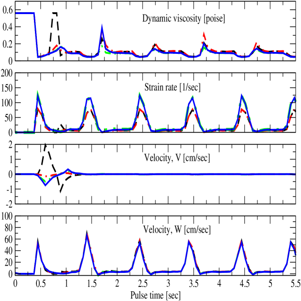
Figure 1: Test of numerical convergence. Time-dependent dynamic viscosity, strain rate and velocity components V and W. Results for a vessel of simple geometry - cylinder type, for a specific spatial point inside the cylinder - the middle point. No turbulence effects are involved in these simulations with the realistic non-Newtonian viscosity of human blood. Black dashed line: calculations with 0.08 size for all cells flow3d , red dot-dashed line with 0.07, green double dot - dashed line with 0.065, and blue bold line calculations with 0.062 size for all cells.

Time-dependent results for pressure, strain rate and velocity components $V$ and $W$ are presented in Fig. 1. The turbulent effects are not taken into account. We chose to present only one precise geometrical point for comparison purposes: the middle point: $r=\theta=0$, and $Z=4.0$ cm. The data for Fig. 1. were obtained with the non-Newtonian model of human blood. We refer the reader to the comments provided for the figure. We were able to closely replicate the values for all previous cell sizes flow3d and obtain almost identical values, for example for pressure, wall shear stress and other parameters, for 0.065 and 0.062 cell sizes flow3d . This means, that the convergence has been achieved.

Next, it would be very interesting to compare the results calculated with and without the turbulent effect. To support this endeavor we use the realistic non-Newtonian model of blood viscosity, the pulsatile flow, and the size of computation cells at which convergence has been achieved, that is the 0.062 size for all computational cells flow3d .

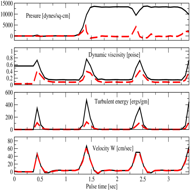
Figure 4: Results for pressure, dynamic viscosity, turbulent energy and velocity W. Time-dependent results for the middle point of the cylinder. Bold black line calculations with non-Newtonian viscosity of the human blood; red dashed line with its Newtonian approximation.

The results are presented in Fig. 2. As we see from Fig. 2 the effect of the turbulence is significant, particularly in regard to dynamic viscosity and strain rate. This result means that in the case of pulsatile flows and non-Newtonian viscosity the turbulent term should be taken into account. In Fig. 3 we separately show the results for the pulsatile pressure distribution and the turbulent energy, again using the middle point of the cylinder. Finally, it would also be very interesting to make a comparison between the results calculated using both a Newtonian and non-Newtonian viscosity. However, as in previous simulations, we will apply the pulsatile flow with the turbulence included, since it has proved to be important. The results are shown in Fig. 4. As one can see, we obtain significant differences between these two calculations. We specifically observed that for the pressure distribution, dynamic viscosity and turbulent energy, we obtained significant disagreements.

Thus, we arrive at the important conclusion: within a time-dependent (pulsatile) flow of human blood it is necessary to take into account turbulence and non-Newtonian viscosity.

III.2 Hemodynamics in the coronary bifurcation

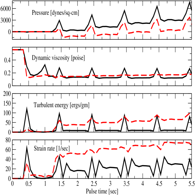
Figure 5: Time-dependent results for a vessel with bifurcation. Pulsatile blood flow, non-Newtonian viscosity, and the turbulence effect is included. Bold black line: results for the far right outflow side $z=0.0$; red dashed line results for the farthest up outflow side $y=0.0$

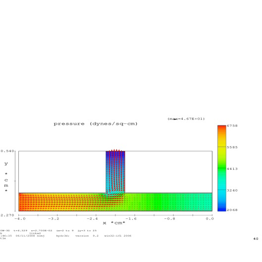
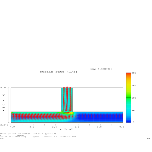
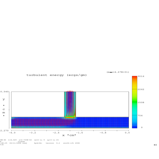
Figure 6: The figures are 2D-plots showing the blood flow in the bifurcated vessels for only one precise moment of the discretized time $t_{i}=4.329$ sec, the corresponding index is $i=40$. Upper plot represents the result for the pressure distribution in the bifurcation, and the pressure ranges from 2068 dynes/sq-cm to 6758 dynes/sq-cm. The middle plot represents the results for the strain rate distribution and the lower plot shows results for the turbulent energy in the bifurcation. The range of the values is also shown.

Below we show the result of our subsequent simulation involving a 90^∘ bifurcated coronary artery in Figs. 5 and 6. The geometrical model of the bifurcation consisted of a 90^∘ intersection of two cylinders. This model represents the bifurcation between the left anterior descending coronary artery and the circumflex coronary artery. In our opinion, in the case of pulsatile flow it is more interesting to present results in a time-dependent way. This method can provide a wider picture of highly non-stationary flow systems. In this paper, because of space limitations, we just included time-dependent results for pressure, dynamic viscosity, turbulent energy, and strain rate. However, we understand, that results which depend on spatial coordinates $(r,\theta,Z)$ for a few fixed moments of time are also highly useful.

In the case of the bifurcation shown in Fig. 5, we report the results for only two spatial points, which are the two outflow sides: the far right side and the farthest upper side of the bifurcation. The length of the lower horizontal vessel is 4 cm and its diameter is 0.54 cm. The length of the upper vertical vessel is 1.2 cm and its diameter is 0.4 cm. These sizes are consistent with average size human vessels.

In Fig. 5 blood flows in from the left to the right with the imposed initial velocity profile taken from Table 1. The pressure, strain rate and turbulent energy distributions are shown for only one specific time moment $t$=4.329 s. The velocity vectors are also shown on these plots.

Further, Fig. 6 represents our time-dependent results for the two outflow sides mentioned above. These results are for pressure, dynamic viscosity, turbulent energy and strain rate. The bold black lines are the results for the right outflow side, and the red dashed lines are the results for the farthest upper side (see comments to Fig. 6). In conclusion, the main goal of these calculations is to adopt them to investigate a case in which a stent 77 is implanted in the bifurcation area.

III.3 Blood flow in aortic arch

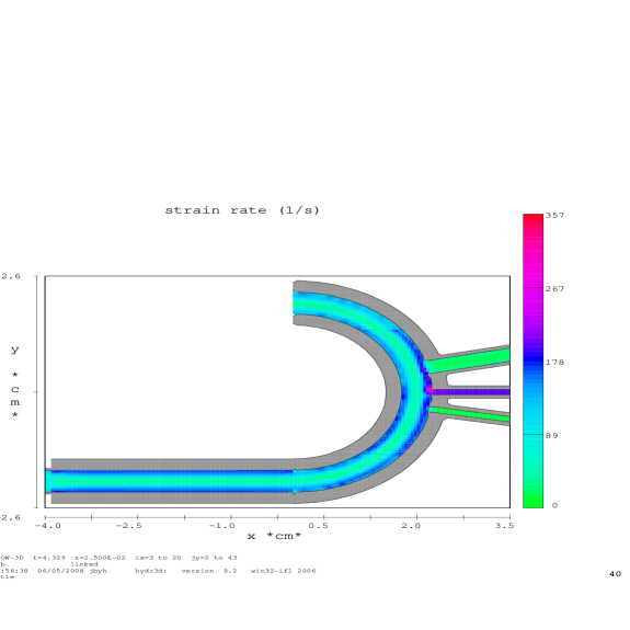
Figure 7: Blood flow in the aortic arch. These two plots represent the full 2D-picture of the geometry used in these simulations. Shaded results for the strain rate are also shown, the bars on the right show the values. Results are for two specific moments of the time $t_{40}$ = 4.329 sec and $t_{41}$ = 4.440 sec. The values of the strain rate distribution range from 0.0 1/sec to 357.0 1/sec (upper plot) and from 0.0 to 671 1/sec (lower plot). The maximum values of the strain rate are localized in the region inside the arch. Blood flows from right to left in both pictures.

The geometry of the blood simulations inside the human aortic arch is shown in Fig. 7. On the top of the aortic arch three arteries are included. These arteries deliver the blood to the carotid artery and then to the brain. This configuration only models and approximately represents the real aortic arch. One of the goals of our simulations is to reveal the physics of the blood flow dynamics in this important portion of the human cardiovascular system.

The aortic arch is represented as a curved tube. The outer radius of the tube is 2.6 cm. A straight vessel (tube) is also merged to the arch. The length of the straight tube is about 4 cm. Again, the thickness of the wall is 0.03 cm, and the inner radius of the tube is $r=0.34$ cm. Once again we are using the Cartesian coordinate system. We also carried out a convergence test. To better represent the shape of the arch we applied five Cartesian sub-coordinate systems in our FLOW3D simulations. After the discretization the total number of all cubic cells reached about 900,000. It is important to mention here, that we again obtained full numerical convergence. In this work we computed pressure, velocity and strain rate distributions in the arch, while the human blood is treated as a non-Newtonian liquid and while the realistic pulsatile blood flow is used.

In Fig. 7 we present the results of strain rate distributions inside the arch for two specific time moments. At the most left point, which is the inlet, we specify the pulsatile velocity source as the initial condition, that is the data from table 1 are used. From the general theory of fluid mechanics landau it is possible to determine together with the blood density and viscosity, and spatial geometries, the dynamics of the blood according to the Navier-Stokes equation and its boundary conditions. Small vectors indicate the blood velocity. As can be seen from Fig. 7 blood flows from left to right in direction. However, because of pulsatility blood flows in the opposite direction too.

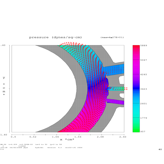
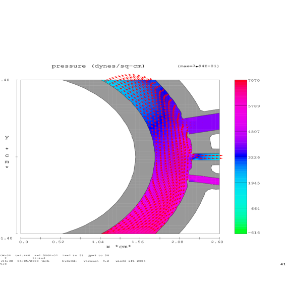
Figure 8: These two plots represent in more detail the region of the arch together with shaded results for the pressure distribution. The bars on the right show the values. These results are for two specific moments of the time $t_{40}$ = 4.329 sec and $t_{41}$ = 4.440 sec, where the pressure ranges from 957 dynes/sp-cm to 5889 dynes/sq-cm (upper plot), and from -616 dynes/sq-cm to 7070 dynes/sq-cm (lower plot).

The values of the strain rate are also shown. These values are strongly oscillating. From the plots one can conclude that in the region of the arch the strain rate values become much larger than in the region of the straight vessel. This result represents clear evidence that in this part of the human vascular system atherosclerotic plaques should localize less than in the straight vessels. However, the higher wall shear stress values in the aortic arch could be the reason for sudden mechanical disruption of the arterial wall in this part of the human vascular system. These results are consistent with laboratory and clinical observations. In Fig. 8 we depict the pressure distribution in the arch.

IV Conclusion

In this work we applied computational fluid dynamics techniques to support pulsatile human blood flow simulations through different shape/size vessels and the aortic arch. The realistic blood pulse has been adopted and applied from work greece2007 . The geometrical size of the vessels and the aortic arch have been selected to match the average real values. Human blood was treated in two different ways: (a) as a Newtonian liquid when the viscosity of the blood has a constant value, and (b) as a non-Newtonian liquid with the viscosity value represented by the equation (9). The numerical coefficients in (9) have been taken from work 1991 .

It is always difficult to obtain a steady-state cycle profile and stable computational results at the very beginning of time-dependent simulations. However, after a short stabilization period a steady-state cycle profile can be obtained. In our simulations we used up to 5.5 pulse cycles to reach complete steady state profiles. We obtained valid results for pressure, wall shear stress distribution and other physical parameters, such as the three velocity components of blood flow. All of these were shown in Figs. 1 and 2.

Our simulations showed that the FLOW3D program is capable of providing stable numerical results for all geometries included in this work. The time-dependent mathematical convergence test has been successfully carried out. Particular attention has been paid to this aspect of the calculations. It is a well known fact that fluid dynamics equations can have unstable solutions landau . Therefore, numerical convergence has been tested and confirmed in this work.

The result of computer simulations of blood flow in vessels for three different geometries have been presented. For pressure, strain rate and velocity component distributions we found significant disagreements between our results obtained with the realistic non-Newtonian treatment of human blood and the widely used method in literature: a simple Newtonian approximation.

Our results are in good agreement with the conclusions of works chn04 ; chn06 , where the authors also obtained significant differences between their results calculated with and without the non-Newtonian effect of blood viscosity. However, the recent work austr07 should be mentioned, in which the authors performed 2-dimensional simulations of human blood flow through the carotid artery with and without the non-Newtonian effect of the viscosity. They did not find any substantial differences in their results. But in the paper india08 , where the authors also performed simulations for the carotid artery, only the non-Newtonian viscosity was used.

Next, the influence of a possible turbulent effect has also been investigated in this work. It was found that the effect is important. We believe, that the physical reason of this phenomena lies in the strong pulsatility of the flow and in the non-Newtonian viscosity of the blood. The contribution of the turbulence is most significant in the area of bifurcated vessels.

Finally, a significant increase of the strain rate and, the wall shear stress distribution, is found in the region of the aortic arch. This computational result provides additional evidence to support recent clinical and laboratory observations that this part of the human cardiovascular system is under higher risk of disruption carter2001 ; poch2006 . In future works it would be interesting to include the elasticity of the walls of the aortic arch pre94 and other vessels.

In conclusion, we would like to specifically point out, that the developments in this work can be directly applied to even more interesting and very important situations such as when a stent is implanted inside a vessel 77 . In this case, for example, it would be very useful to determine blood flow disturbance, the pressure distribution, strain rate and values of other physical parameters. The results of this work should allow us to determine the optimal size and shape of effective stents. As we mentioned in the Introduction some research groups are carrying out laboratory and computer simulations of blood flow through vessels with implanted stents 77 . It is very difficult to underestimate the value of these works.

V Appendix

For a variable dynamic viscosity $\mu$, the viscous accelerations are

$$\rho V_{F}f_{x}=w^{s}_{x}-[\frac{\partial}{\partial x}(A_{x}\tau_{xx})+R\frac{\partial}{\partial y}(A_{y}\tau_{xy})+\frac{\partial}{\partial z}(A_{z}\tau_{xz})+\frac{\xi}{x}(A_{x}\tau_{xx}-A_{y}\tau_{yy})]$$ (10)

$$\rho V_{F}f_{y}=w^{s}_{y}-[\frac{\partial}{\partial x}(A_{x}\tau_{xy})+R\frac{\partial}{\partial y}(A_{y}\tau_{yy})+\frac{\partial}{\partial z}(A_{z}\tau_{yz})+\frac{\xi}{x}(A_{x}+A_{y}\tau_{xy})]$$ (11)

$$\rho V_{F}f_{z}=w^{s}_{z}-[\frac{\partial}{\partial x}(A_{x}\tau_{xz})+R\frac{\partial}{\partial y}(A_{y}\tau_{yz})+\frac{\partial}{\partial z}(A_{z}\tau_{zz})+\frac{\xi}{x}(A_{x}\tau_{xz})],$$ (12)

where

$$\tau_{xx}=-2\mu\left(\frac{\partial u}{\partial x}-\frac{1}{3}\left(\frac{\partial u}{\partial x}+R\frac{\partial v}{\partial y}+\frac{\partial w}{\partial z}+\frac{\xi u}{x}\right)\right)$$ (13)

$$\tau_{yy}=-2\mu\left[R\frac{\partial v}{\partial x}+\xi\frac{u}{x}-\frac{1}{3}\left(\frac{\partial u}{\partial x}+R\frac{\partial v}{\partial y}+\frac{\partial w}{\partial z}+\frac{\xi u}{x}\right)\right]$$ (14)

$$\tau_{zz}=-2\mu\left(\frac{\partial w}{\partial z}-\frac{1}{3}\left(\frac{\partial u}{\partial x}+R\frac{\partial v}{\partial y}+\frac{\partial w}{\partial z}+\frac{\xi u}{x}\right)\right)$$ (15)

$$\tau_{xy}=-\mu\left(\frac{\partial v}{\partial x}+R\frac{\partial u}{\partial y}-\frac{\xi v}{x}\right)$$ (16)

$$\tau_{xz}=-\mu\left(\frac{\partial u}{\partial z}+\frac{\partial w}{\partial x}\right)$$ (17)

$$\tau_{yz}=-\mu\left(\frac{\partial v}{\partial z}+R\frac{\partial w}{\partial y}\right).$$ (18)

In the above equations (10)-(12) the terms $w^{s}_{x},w^{s}_{y}$ and $w^{s}_{z}$ are wall shear stresses. If these terms are equal to zero, there is no wall shear stress. This is because the remaining terms contain the fractional flow areas $(A_{x},A_{y},A_{z})$ which vanish at the walls flow3d .

Table 1: Time-dependent velocity profile at the vessel inlet. The velocity vector is directed exactly over the axis of the tube. Blood velocities $v_{i}$ are given in cm/sec versus the corresponding time moments $t_{i}$ in sec ($i=1,2,...,30$). Results taken from Fig. 2 of work greece2007 .

$t_{i}$	$v_{i}$	$t_{i}$	$v_{i}$	$t_{i}$	$v_{i}$
0.0	1.5	0.35	27.5	0.625	-4.0
0.015	1.6	0.385	47.0	0.65	-3.0
0.035	2.5	0.39	49.0	0.7	2.1
0.075	2.0	0.4	50.0	0.725	2.6
0.1	2.6	0.41	49.0	0.75	2.1
0.15	2.0	0.415	47.0	0.8	2.6
0.2	2.6	0.45	33.0	0.85	3.2
0.23	2.2	0.5	14.5	0.9	2.6
0.25	3.6	0.55	1.9	0.95	2.2
0.3	12.0	0.4	50.0	1.0	1.5

FIG. 1. Test of numerical convergence. Time-dependent dynamic viscosity, strain rate and velocity components V and W. Results for a vessel of simple geometry - cylinder type, for a specific spatial point inside the cylinder - the middle point. No turbulence effects are involved in these simulations with the realistic non-Newtonian viscosity of human blood. Black dashed line: calculations with 0.08 size for all cells flow3d , red dot-dashed line with 0.07, green double dot - dashed line with 0.065, and blue bold line calculations with 0.062 size for all cells.

FIG. 2. Time-dependent results for a specific geometrical point inside the cylinder: the middle point. Black dashed line: simulations without taking into account the turbulence; red bold line results with the turbulence. The non-Newtonian viscosity is taken into account.

FIG. 3. Time-dependent results for pressure and the turbulent energy in the middle point of the cylinder. The non-Newtonian viscosity.

FIG. 4. Results for pressure, dynamic viscosity, turbulent energy and velocity W. Time-dependent results for the middle point of the cylinder. Bold black line calculations with non-Newtonian viscosity of the human blood; red dashed line with its Newtonian approximation.

FIG. 5. Time-dependent results for a vessel with bifurcation. Pulsatile blood flow, non-Newtonian viscosity, and the turbulence effect is included. Bold black line: results for the far right outflow side $z=0.0$; red dashed line results for the farthest up outflow side $y=0.0$.

FIG. 6. The figures are 2D-plots showing the blood flow in the bifurcated vessels for only one precise moment of the discretized time $t_{i}=4.329$ sec, the corresponding index is $i=40$. Upper plot represents the result for the pressure distribution in the bifurcation, and the pressure ranges from 2068 dynes/sq-cm to 6758 dynes/sq-cm. The middle plot represents the results for the strain rate distribution and the lower plot shows results for the turbulent energy in the bifurcation. The range of the values is also shown.

FIG. 7. Blood flow in the aortic arch. These two plots represent the full 2D-picture of the geometry used in these simulations. Shaded results for the strain rate are also shown, the bars on the right show the values. Results are for two specific moments of the time $t_{40}$ = 4.329 sec and $t_{41}$ = 4.440 sec. The values of the strain rate distribution range from 0.0 1/sec to 357.0 1/sec (upper plot) and from 0.0 to 671 1/sec (lower plot). The maximum values of the strain rate are localized in the region inside the arch. Blood flows from right to left in both pictures.

FIG. 8. These two plots represent in more detail the region of the arch together with shaded results for the pressure distribution. The bars on the right show the values. These results are for two specific moments of the time $t_{40}$ = 4.329 sec and $t_{41}$ = 4.440 sec, where the pressure ranges from 957 dynes/sp-cm to 5889 dynes/sq-cm (upper plot), and from -616 dynes/sq-cm to 7070 dynes/sq-cm (lower plot).

Figures

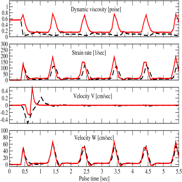
Figure 2: Time-dependent results for a specific geometrical point inside the cylinder: the middle point. Black dashed line: simulations without taking into account the turbulence; red bold line results with the turbulence. The non-Newtonian viscosity is taken into account.

References

- (1) L.Waite, Biofluid Mechanics in Cardiovascular Systems, Mc-Graw-Hill Professional Publishing, 2005.
- (2) S. Dhein, M. Delmar, and F.W. Mohr, Practical Methods in Cardiovascular Research, Springer-Verlag New-York, LLC, 2005.
- (3) Y.C. Fung, Biomechanics, Springer, 1993.
- (4) L.D. Landau, E.M. Lifshitz, Fluid Mechanics, Volume 6, Pergamon Press Ltd., 1959.
- (5) J.B. Grotberg, O.E. Jensen, Biofluid Mechanics in Flexible Tubes, Ann. Rev. Fluid Mech. 36, 121-147 (2004).
- (6) C.A. Taylor, M.T. Draney, Experimental and Computational Methods in Cardiovascular Fluid Mechanics, Annual Review of Fluid Mechanics 36, 197-231 (2004).
- (7) Y. Huo, G.S. Kassab, Pulsatile Blood Flow in the Entire Coronary Arterial Tree: Theory and Experiment, Am. J. Physiol. Heart Circ. Physiol 291: 1074 (2006).
- (8) C.S. Peskin, Numerical Analysis of Blood Flow in the Heart, Journal of Computational Physics, 25 (3 , Nov.1977), 220-252 (1977).
- (9) Y.I. Cho, K.R. Kensey, Effects of the non-Newtonian viscosity of blood on flows in a diseased arterial vessel. Part 1: Steady Flows, Biorheology 28, 241-262 (1991).
- (10) B.M. Johnston, P.R. Johnston, S. Corney, and D. Kilpatrick, Non-Newtonian Blood Flow in Human Right Coronary Arteries: Steady State Simulations, J. of Biomech. 37, 709 (2004).
- (11) J. Chen, X.-Y, Lu, Numerical investigation of the non-Newtonian pulsatile blood flow in a bifurcation model with a non-planar branch, J. of Biomechanics 37, 1899-1911 (2004).
- (12) L. Morris, P. Delassus, A. Callanan, M. Walsh, F. Wallis, P. Grace, and T. McGoughlin, 3-D Numerical Simultation of Blood Flow Throught Models of the Human Aorta, J. of Biomech. Engineering 127, 767-775 (2005).
- (13) L. Morris, P. Delassus, M. Walsh, and T. McGloughlin, A mathematical model to predict the in vivo pulsatile drag forces acting on bifurcated stent grafts used in endovascular treatment of abdominal aortic aneurysms (AAA): J. of Biomechanics 37, 1087-1095 (2004).
- (14) J. Chen, X.-Y, Lu, Numerical investigation of the non-Newtonian pulsatile blood flow in a bifurcation model with a non-planar branch, Journal of Biomechanics 39, 818-832 (2006).
- (15) N. Duraiswamy, R.T. Schoephoerster, M.R. Moreno, J. E. Moore Jr., Stented Artery Flow Patterns and Their Effects on the Artery Wall, Ann. Rev. of Fluid Mechanics 39, 357-382 (2007).
- (16) K. Mukundakrishnan, P.S. Ayyaswamy, D.M. Eckmann, Finite-sized gas bubble motion in a blood vessel: Non-Newtonian effects, Phys. Rev. E 78, art. numb. 036303 (2008).
- (17) R.A. Sultanov, D. Guster, B. Engelbrekt, and R. Blankenbecler, A Full Dimensional Numerical Study of Pulsatile Human Blood Flow in Aortic Arch, Proceedings of the 2008 International Conference on Bioinformatics and Computational Biology, Vol. 2, p.p. 437-443, Eds. H.M. Arabnia, M.Q. Yang, J.Y. Yang, CSREA Press-WORLDCOMP 2008.
- (18) R.A. Sultanov, D. Guster, B. Engelbrekt, and R. Blankenbecler, 3D Computer simulations of pulsatile human blood flows in vessels and in aortic arch: investigation of non-Newtonian characteristics of human blood, Proceedings of the 2008 11-th IEEE International Conference on Computational Science and Engineering, p.p. 479-485, IEEE Comp. Soc. 2008.
- (19) A.O. Frank, P.W. Walsh, and J.E. Moore Jr., Computational Fluid Dynamics and Stent Design, Artificial Organs 26(7), 614 (2002).
- (20) T. Seo, L.G. Schachter, A.I. Barakat, Computational Study of Fluid Mechanical Disturbance Induced by Endovascular Stents, Annals of Biomed. Engineering 33 (4), 444-456 (2005).
- (21) N. Benard, R. Perrault, D. Coisne, Computational Approach to Estimating the Effects of Blood Properties on Changes in Intra-Stent Flow, Annals of Biomed. Engineering 34 (8), 1259-1271 (2006).
- (22) I. Faik, R. Mongrain, R.L. Leask, J. Rodes-Cabau, E. Larose, O. Bertrand, Time-Dependent 3D Simulations of the Hemodynamics in a Stented Coronary Artery, Biomedical Materials 2 (1), art. no. S05, S28-S37 (2007).
- (23) R.K. Banerjee, S.B. Devarakonda, D. Rajamohan, L.H. Back, Developed Pulsatile Flow in a Deployed Coronary Stent, Biorheology 44 (2), 91-102 (2007).
- (24) FLOW-3D Users Manual, Version 9.2, Flow Science, Santa Fe, New Mexico, 2007.
- (25) Y. Papaharilaou, J.A. Ekaterinaris, E. Manousaki, A.N. Katsamouris, A Decoupled Fluid Structure Approach for Estimating Wall Stress in Abdominal Aortic Aneurysms, J. Biomechanics 40, 367-377 (2007).
- (26) J. Boyd, J.M. Buick, Comparison of Newtonian and non-Newtonian Flows in a Two-Dimensional Carotid Artery Model Using the Lattice Boltzmann Method, Physics in Medicine and Biology 52, 6215 (2007).
- (27) R. Agarwal, V.K. Katiyar, P. Pradhan, A mathematical modeling of pulsatile flow in carotid artery bifurcation, Intern. J. of Engineering Science (in press).
- (28) Y.M. Carter, R.C. Karmy-Jones, D.C. Oxorn, G.S. Aldea, Traumatic Disruption of the Aortic Arch, European J. Cardio-thoracic Surgery, 20, 1231 (2001).
- (29) A. Pochettino, J.E. Bavaria, Aortic Dissection, in Book: Mastery of Cardiothoracic Surgery, Eds. L.R. Kaiser, I.L. Kron, T.L. Spray, Publisher: Lippincott Williams and Wilkins, September 2006.
- (30) H. Fang, Z. Lin, Z. Wang, Lattice Boltzmann Simulation of Viscous Fluid Systems with Elastic Boundaries, Phys. Rev. E 57, R25-R28 (1998).