Isotope effect and the role of phonon in the Fe-based superconductors

Abstract

We studied the isotope effect of phonon in the Fe-based superconductors using a phenomenological two band model for the sign-changing s-wave ($\pm$s-wave) state. Within this mean-field model, we showed that the large isotope effect is not inconsistent with the $\pm$s-wave pairing state and its high transition temperature. In principle, a large phonon isotope coefficient $\alpha$ implies a large phonon coupling constant. However, the asymmetric density of states (DOS) between two bands substantially enhances the value of $\alpha$, so that a moderate value of the phonon coupling constant ($\lambda_{\rm ph}\approx 0.4$) can produce a very large value of $\alpha$ ($\approx 0.4$) as well as a high transition temperature together with an antiferromagnet (AFM)-induced interaction.

Recent discovery of the Fe-based superconductors by Kamihara et al. Kamihara ; PhysToday08 , has greatly spurred the research activity of unconventional superconductivity. Regarding the pairing mechanism and symmetry of theses new superconducting (SC) materials, there are already numerous experimental and theoretical investigations. Since the first theoretical proposal of the $\pm$s-wave state by Mazin et al., Mazin08 as a best pairing state in the Fe-based superconductors (SCs), several subsequent theoretical studies Kuroki ; Eremin ; DHLee ; Bang08a supported this idea. Experiments such as ARPES Ding and penetration depth measurements pene unanimously indicate a full gap around the Fermi surfaces (FSs) consistent with a s-wave gap state. Then the nuclear spin-lattice relaxation rate $1/T_{1}$ T1 , which is seemingly consistent with a nodal gap state such as a d-wave gap, provided a strong evidence of the sign-changing nature of the gaps on different bands, so that actually strengthened the case of the $\pm$s-wave state Bang08a ; Bang08b ; recent .

As to the pairing glue, most researchers at the moment tend to believe an electronic origin rather than a phonon origin paring Kuroki ; Bang08a ; Eremin ; DHLee ; Tesanovic . In particular, an antiferromagnetic (AFM) correlation induced interaction appears to be the most natural pairing glue in view of the common SDW instability at around $\sim 150$ K and the overall phase diagram with doping in this series of Fe pnictides neutron . It is shown by several authors that the AFM-induced potential, when combined with the unique band structure (or the FS topology) of the Fe pnictides, naturally leads to the $\pm$s-wave state as the best pairing solution Kuroki ; Bang08a ; Eremin ; DHLee .

However, Liu et al. isotope recently measured isotope effect on $T_{c}$ with a substitution of ⁵⁶Fe by ⁵⁴Fe in Ba_1-xK_xFe₂As₂, and reported a unexpectedly large isotope coefficient $\alpha$ ($\sim 0.4$). This observation, if confirmed, is drastically perpendicular to the current line of thought for the pairing mechanism of the Fe-based SCs. Theoretical investigations about the electron-phonon coupling in these materials are yet only a few. Boeri et al. Boeri calculated a very weak electron-phonon coupling constant ($\lambda_{\rm ph}<0.2$) – the value averaged over the Brillouin Zone (BZ). Eschrig Eschrig argued that the proper electron-phonon coupling is not the averaged coupling constant but the one of a particular phonon mode, i.e., in-plane Fe-breathing mode, which may have a large electron-phonon coupling constant.

Besides theoretical investigations, the experimental fact is that all Fe pnictides, either RFeAsO (R= La, Ce, and Nd) or AKFe₂As₂ (A=Ba and Sr) compounds, display the structural instability from tetragonal to orthorhombic symmetry and it always occurs at temperatures very near the SDW transition temperatures structure . It implies, at least, two things: (1) the lattice degrees of freedom (structural instability) and the spin degrees of freedom (magnetic instability) are not independent; (2) this structural instability is not a Jahn-Teller-type instability of the Fe 3d-electrons but is closely related with the metallicity of the Fe 3d-electrons Tesanovic . Therefore, the issue of the electron-phonon coupling in the Fe pnictides needs to be further investigated.

With this motivation, in this paper, we studied the isotope effect and the role of phonon using a phenomenological model for the $\pm$s-wave pairing state. The details of the model can be found in Ref.Bang08a and here we briefly sketch the essential ingredients for our purpose. The model consists of two bands: one hole band centered around $\Gamma$ point and one electron band centered around $M$ point in the reduced Brillouin Zone (BZ) scheme, and has a phenomenological pairing interaction, induced from an AFM correlation, hence peaking around $(\pi,\pi)$ momentum exchange. In this paper, we add a phonon interaction to this model. Because our purpose of this paper is to study the isotope effect of phonon when the total interaction gives rise to the $\pm$s-wave pairing state, we assume only a general condition of the phonon interaction and vary the basic parameters of the phonon interaction such as the coupling strength $\lambda_{\rm ph}$ and the characteristic phonon frequency $\omega_{\rm ph}$.

The Hamiltonian is written as

$$H = \sum_{k\sigma}\epsilon_{h}(k)h^{{\dagger}}_{k\sigma}h_{k\sigma}+\sum_{k\sigma}\epsilon_{e}(k)e^{{\dagger}}_{k\sigma}e_{k\sigma}$$ (1)

$$+\sum_{kk^{{}^{\prime}}\uparrow\downarrow}V_{\rm AFM}(k,k^{{}^{\prime}})h^{{\dagger}}_{k\uparrow}h^{{\dagger}}_{-k\downarrow}h_{k^{{}^{\prime}}\downarrow}h_{-k^{{}^{\prime}}\uparrow}$$

$$+\sum_{kk^{{}^{\prime}}\uparrow\downarrow}V_{\rm AFM}(k,k^{{}^{\prime}})e^{{\dagger}}_{k\uparrow}e^{{\dagger}}_{-k\downarrow}e_{k^{{}^{\prime}}\downarrow}e_{-k^{{}^{\prime}}\uparrow}$$

$$+\sum_{kk^{{}^{\prime}}\uparrow\downarrow}V_{\rm AFM}(k,k^{{}^{\prime}})h^{{\dagger}}_{k\uparrow}h^{{\dagger}}_{-k\downarrow}e_{k^{{}^{\prime}}\downarrow}e_{-k^{{}^{\prime}}\uparrow}$$

$$+\sum_{kk^{{}^{\prime}}\uparrow\downarrow}V_{\rm AFM}(k,k^{{}^{\prime}})e^{{\dagger}}_{k\uparrow}e^{{\dagger}}_{-k\downarrow}h_{k^{{}^{\prime}}\downarrow}h_{-k^{{}^{\prime}}\uparrow}$$

$$+\sum_{kk^{{}^{\prime}}\uparrow\downarrow}V_{\rm ph}(k,k^{{}^{\prime}})h^{{\dagger}}_{k\uparrow}h^{{\dagger}}_{-k\downarrow}h_{k^{{}^{\prime}}\downarrow}h_{-k^{{}^{\prime}}\uparrow}$$

$$+\sum_{kk^{{}^{\prime}}\uparrow\downarrow}V_{\rm ph}(k,k^{{}^{\prime}})e^{{\dagger}}_{k\uparrow}e^{{\dagger}}_{-k\downarrow}e_{k^{{}^{\prime}}\downarrow}e_{-k^{{}^{\prime}}\uparrow}$$

where $\epsilon_{h,e}(k)$ are the dispersions of the hole band and electron bands, respectively, representing two main bands in the Fe pnictides. The details of the dispersions are not important for our purpose except the density of states (DOS) of each band, $N_{h}$ (hole band) and $N_{e}$ (electron band), respectively. $h^{{\dagger}}_{k\sigma}$ and $e^{{\dagger}}_{k\sigma}$ are the electron creation operators on the hole and the electron bands, respectively. As mentioned previously, $V_{\rm AFM}(k,k^{{}^{\prime}})$ is the AFM-induced pairing potential, which is all repulsive in momentum space, and $V_{\rm ph}(k,k^{{}^{\prime}})$ is the phonon interaction, which is all attractive in momentum space.

The minimum characteristics of the interactions to promote the $\pm$s-wave gap solution are: $V_{\rm AFM}(k,k^{{}^{\prime}})$, peaking around $(\pi,\pi)$ momentum exchange, should have a stronger interband interaction than the intraband one; and $V_{\rm ph}(k,k^{{}^{\prime}})$, being stronger for small momentum exchange, should have a stronger intraband interaction than the interband one. The latter requirement for the phonon interaction is already included in the Hamiltonian by not including the interband terms like $V_{\rm ph}(k,k^{{}^{\prime}})e^{{\dagger}}_{k\uparrow}e^{{\dagger}}_{-k\downarrow}h_{k^{{}^{\prime}}\downarrow}h_{-k^{{}^{\prime}}\uparrow}$ and its hermitian conjugate. This assumption of the phonon interaction is indeed the property of the main phonons in Fe pnictides Boeri . If the phonon interaction were absolutely momentum independent, it would have null effect for the $\pm$s-wave pairing.

For simplicity of the analysis but without loss of generality, we only need the FS-averaged interactions: for the AFM-induced interactions such as $V_{\rm AFM}^{he}=<<V_{\rm AFM}(k_{h},k_{e})>>_{k_{h},k_{e}}$, $V_{\rm AFM}^{hh}=<<V_{\rm AFM}(k_{h},k^{\prime}_{h})>>_{k_{h},k^{\prime}_{h}}$, etc. and similarly for the phonon interactions such as $V_{\rm ph}^{hh}=-<<V_{\rm ph}(k_{h},k^{\prime}_{h})>>_{k_{h},k^{\prime}_{h}}$ and $V_{\rm ph}^{ee}=-<<V_{\rm ph}(k_{e},k^{\prime}_{e})>>_{k_{e},k^{\prime}_{e}}$. Notice that, in these definitions, we absorbed the signs of the interactions and therefore all $V_{\rm AFM}^{ab}$ and $V_{\rm ph}^{ab}$ are positive values. Also assuming the $\pm$s-wave solution we fix the signs of the s-wave gaps as $\Delta_{h}=|\Delta_{h}|$ on the hole band and $\Delta_{e}=-|\Delta_{e}|$ on the electron band, respectively. The coupled $T_{c}$-equations are written as

$$\Delta_{h} = -\bigl{[}V_{\rm AFM}^{hh}N_{h}\chi^{\rm AFM}-V_{\rm ph}^{hh}N_{h}\chi^{\rm ph}\bigr{]}\Delta_{h}$$

$$+\bigl{[}V_{\rm AFM}^{he}N_{e}\chi^{\rm AFM}\bigr{]}\Delta_{e},$$

$$\Delta_{e} = -\bigl{[}V_{\rm AFM}^{ee}N_{e}\chi^{\rm AFM}-V_{\rm ph}^{ee}N_{e}\chi^{\rm ph}\bigr{]}\Delta_{e}$$ (3)

$$+\bigl{[}V_{\rm AFM}^{eh}N_{h}\chi^{\rm AFM}\bigr{]}\Delta_{h}.$$

The pair susceptibilities $\chi^{\rm AFM}$ and $\chi^{\rm ph}$ at $T=T_{c}$ are defined as

$$\chi(T_{c})^{\rm AFM,ph} = \int_{0}^{\omega_{\rm AFM,ph}}\frac{d\xi}{\xi}\tanh\Bigl{[}\frac{\xi}{2T_{c}}\Bigr{]}$$

$$\approx \ln\Bigl{[}\frac{1.14~{}\omega_{\rm AFM,ph}}{T_{c}}\Bigr{]}.$$

where $\omega_{\rm AFM}$ and $\omega_{\rm ph}$ are the cutoff frequencies of the AFM fluctuations and phonon, respectively. The second expression is the well-known BCS approximation valid only when $\omega_{\rm AFM,ph}\gg T_{c}$, otherwise the first expression should be numerically calculated. Equations (2) and (3) with Eq.(4) constitute the $T_{c}$-equation of the $\pm$ s-wave state of the two band model, including phonon pairing interaction as well as the AFM-induced pairing interaction. Before we show the numerical results we can analyze a simple case and gain general insight about the model.

In the case (we call it ”symmetric case”) that $N_{h}=N_{e}$, and $V_{\rm AFM}^{ee}=V_{\rm AFM}^{hh}$ and $V_{\rm ph}^{ee}=V_{\rm ph}^{hh}$ ($V_{\rm AFM}^{he}=V_{\rm AFM}^{eh}$ is always true), we define the dimensionless pairing constants as follows,

$$\lambda_{\rm AFM}^{inter} = N_{h}V_{\rm AFM}^{he}=N_{e}V_{\rm AFM}^{eh}$$ (5)

$$\lambda_{\rm AFM}^{intra} = N_{h}V_{\rm AFM}^{hh}=N_{e}V_{\rm AFM}^{ee}$$ (6)

$$\lambda_{\rm ph} = N_{h}V_{\rm ph}^{hh}=N_{e}V_{\rm ph}^{ee}.$$ (7)

Then, the $T_{c}$-equations are simplified as

$$\Delta_{h}(1+\lambda_{\rm AFM}^{intra}\chi^{\rm AFM}-\lambda_{\rm ph}\chi^{\rm ph}) = \lambda_{\rm AFM}^{inter}\chi^{\rm AFM}\Delta_{e},$$ (8)

$$\Delta_{e}(1+\lambda_{\rm AFM}^{intra}\chi^{\rm AFM}-\lambda_{\rm ph}\chi^{\rm ph}) = \lambda_{\rm AFM}^{inter}\chi^{\rm AFM}\Delta_{h}.$$

The above $T_{c}$-equations can be solved analytically with the BCS approximation of the pair susceptibilities $\chi^{\rm AFM}$ and $\chi^{\rm ph}$, the second expression of Eq.(4), as

$$T_{c}=1.14~{}\omega_{\rm AFM}^{\tilde{\lambda}_{\rm M}}\cdot\omega_{\rm ph}^{\tilde{\lambda}_{\rm ph}}\cdot\exp^{-1/\lambda_{tot}}.$$ (9)

where

$$\lambda_{tot} = (\lambda_{\rm AFM}^{inter}-\lambda_{\rm AFM}^{intra})+\lambda_{\rm ph}$$ (10)

$$\tilde{\lambda}_{\rm M} = (\lambda_{\rm AFM}^{inter}-\lambda_{\rm AFM}^{intra})/\lambda_{tot}$$ (11)

$$\tilde{\lambda}_{\rm ph} = \lambda_{\rm ph}/\lambda_{tot}.$$ (12)

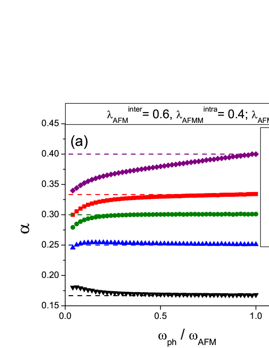
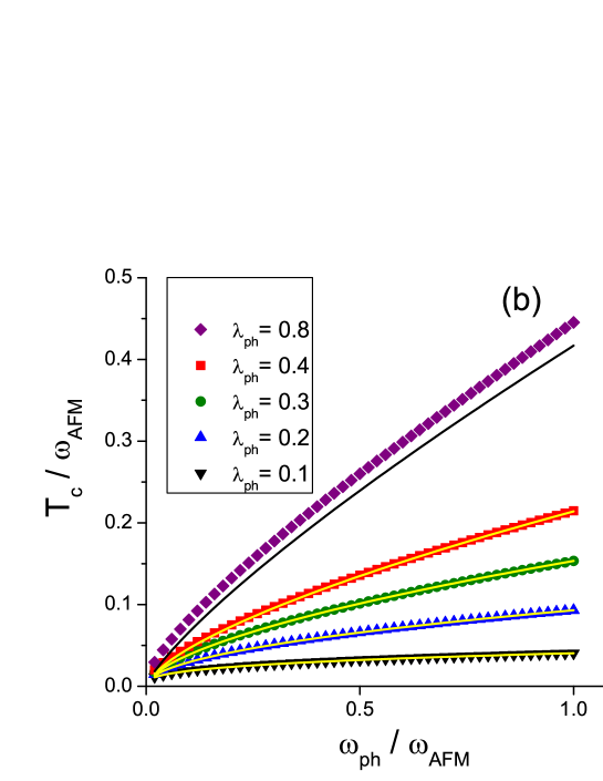
Figure 1: (Color online) Symmetric case ($N_{h}/N_{e}=1.0$). (a) Isotope coefficients $\alpha$ as a function of the phonon cutoff frequency $\omega_{\rm ph}/\omega_{\rm AFM}$ for different phonon coupling constants $\lambda_{\rm ph}=0.1,0.2,0.3,0.4$ and 0.8. (b) Normalized $T_{c}$ vs $\omega_{\rm ph}/\omega_{\rm AFM}$ for the same parameters. Symbols are numerical calculations and lines are the results of Eqs. (9) and (13).

Equations (9) and (10) show that the AFM interaction and the phonon interaction is additive in the exponential form so that $T_{c}$ can be dramatically boosted even with a small value of $\lambda_{\rm ph}$ Bang-HTC . We can also easily read the phonon isotope coefficient $\alpha$ from Eq.(9) as

$$\alpha=\frac{1}{2}\frac{d\ln T_{c}}{d\ln\omega_{\rm ph}}=0.5\times\frac{\lambda_{\rm ph}}{(\lambda_{\rm AFM}^{inter}-\lambda_{\rm AFM}^{intra})+\lambda_{\rm ph}}.$$ (13)

This result conforms with a physical insight, i.e., a large $\alpha$ value means a relatively large phonon coupling compared to the total AFM pairing interaction $\lambda_{\rm AFM}^{eff-tot}=(\lambda_{\rm AFM}^{inter}-\lambda_{\rm AFM}^{intra})$. However, Eq.(9) also shows that a large $\alpha$ value does not necessarily mean the large phonon contribution to the pairing energetics when $\omega_{\rm ph}$ is much smaller than $\omega_{\rm AFM}$.

For the general cases where $N_{h}\neq N_{e}$, and $V_{\rm AFM}^{ee}\neq V_{\rm AFM}^{hh}$ and $V_{\rm ph}^{ee}\neq V_{\rm ph}^{hh}$ (”non-symmetric case”), it is not possible to find an analytic solution of the $T_{c}$-equation. However, an inspection suggests us to generalize Eq.(9) to the non-symmetric case. Equations (9) and (13) can be used as good approximations for $T_{c}$ and $\alpha$ with the definitions of the effective dimensionless coupling constants as follows,

$$\lambda_{\rm AFM}^{inter} = \sqrt{N_{h}N_{e}V_{\rm AFM}^{he}V_{\rm AFM}^{eh}}$$ (14)

$$\lambda_{\rm AFM}^{intra} = \sqrt{N_{h}N_{e}V_{\rm AFM}^{hh}V_{\rm AFM}^{ee}}$$ (15)

$$\lambda_{\rm ph} = \sqrt{N_{h}N_{e}V_{\rm ph}^{hh}V_{\rm ph}^{ee}}.$$ (16)

In the following, we will show numerical results directly obtained from Eqs. (2) and (3) and compare them with the analytic formulas (9) and (13) both for the symmetric and non-symmetric cases.

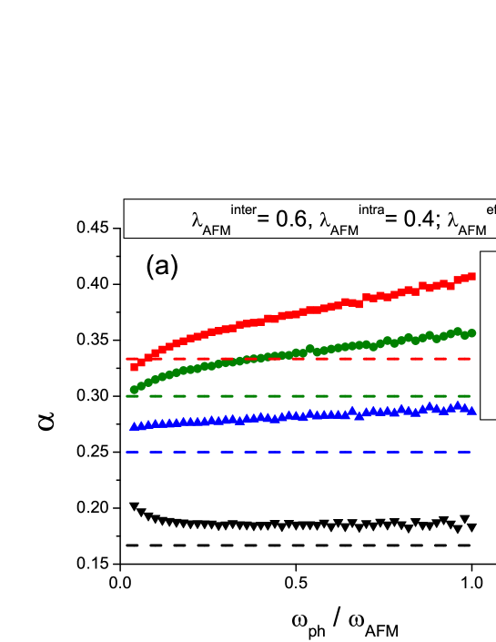
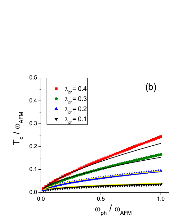
Figure 2: (Color online) Non-symmetric case ($N_{h}/N_{e}=3.0$). (a) Isotope coefficients $\alpha$ as a function of the phonon cutoff frequency $\omega_{\rm ph}/\omega_{\rm AFM}$ for different phonon coupling constants $\lambda_{\rm ph}=0.1,0.2,0.3$ and 0.4. (b) Normalized $T_{c}$ vs $\omega_{\rm ph}/\omega_{\rm AFM}$ for the same parameters. Symbols are numerical calculations and lines are the results of Eqs. (9) and (13).

Fig.1(a) shows the isotope coefficient $\alpha$ of the symmetric case ($N_{h}=N_{e}$). Symbols are the numerical results of Eqs. (2) and (3), and lines are the results of Eq.(13). All the energy scales are normalized by the cutoff frequency of the AFM-fluctuations $\omega_{\rm AFM}$ and we choose moderate strength of dimensionless coupling constants of the AFM-induced potential as $\lambda_{\rm AFM}^{inter}=N_{h}V_{\rm AFM}^{he}=N_{e}V_{\rm AFM}^{eh}=0.6$ and $\lambda_{\rm AFM}^{intra}=N_{h}V_{\rm AFM}^{hh}=N_{e}V_{\rm AFM}^{ee}=0.4$, which yields the effective total magnetic interaction $\lambda_{\rm AFM}^{eff-tot}=0.2$. Fig.1(a) shows that the numerically calculated $\alpha$ (symbols) are in excellent agreement with the analytic results of Eq.(13) when $\omega_{\rm ph}\gg T_{c}$. When this condition is not fulfilled, deviations occurs at low $\omega_{\rm ph}$ where the BCS approximation of the pair susceptibility becomes poor.

The results of Fig.1(a) shows that a large phonon isotope coefficient arises when the phonon coupling strength is much stronger than the magnetic coupling strength and it is in accord with a standard expectation. For example, in the symmetric case, in order to obtain $\alpha\approx 0.4$ (the reported value by Liu et al. isotope ), we need to have $\lambda_{\rm ph}=4\times\lambda_{\rm AFM}^{eff-tot}$ which corresponds to the result of $\lambda_{\rm ph}=0.8$ (purple diamond symbols). If this is the case of reality, then the superconductivity of the Fe pnictides is a phonon driven SC and the AFM-fluctuations merely act as a tipping agent to introduce the $\pi$ phase between two bands widely separated in the BZ. It is not an impossible scenario, but we first need to find an evidence of such a strong phonon coupling in Fe pnictides. If confirmed, the current viewpoint about the pairing mechanism of the Fe-based SCs should completely be changed.

In Fig.2 we show the results of the non-symmetric case ($N_{h}=3N_{e}$). We adjust the parameters to keep the dimensionless coupling constants $\lambda_{\rm AFM}^{inter}=0.6$ and $\lambda_{\rm AFM}^{intra}=0.4$, the same values as in Fig.1. Here $\lambda_{\rm AFM}^{inter,intra}$ are calculated according to the generalized formulas Eqs. (14) and (15). The phonon coupling constants $\lambda_{\rm ph}=0.1,0.2,0.3,0.4$ are also the values according to Eq.(16). The behavior of $\alpha$ is very different compared to the symmetric case: (1) there are systematic deviations of the numerical (exact) results from the analytic (approximate) formula Eq.(13) and the numerically calculated values of $\alpha$ give substantially larger values than the ones of the analytic formula. As a result, a moderate value of $\lambda_{\rm ph}=0.4$ can cause a large isotope coefficient $\alpha\approx 0.4$; (2) with increasing $\omega_{\rm ph}$, there is no saturation of $\alpha$, in particular with large phonon couplings. In contrast, the $T_{c}$ values are rather similar to the symmetric case.

This seemingly inconsistent behavior between $T_{c}$ and $\alpha$ can be most easily understood by comparison of the $\lambda_{\rm ph}=0.4$ results between the symmetric case (Fig.1) and the non-symmetric case (Fig.2). $\alpha$ in the symmetric case quickly saturates to its maximum value (red square symbols in Fig.1(a)) but $\alpha$ in the non-symmetric case gradually increases with $\omega_{\rm ph}$ ( red square symbols in Fig.2(a)). As a result, a large difference of the $\alpha$ value between the two cases is possible when $\omega_{\rm ph}/\omega_{\rm AFM}\rightarrow 1$ while maintaining only slightly enhanced $T_{c}$ (see red square symbols in Fig.1(b) and in Fig.2(b)). Slightly enhanced $T_{c}$ is due to the fact that the asymmetric phonon couplings on the hole band and electron band are slightly more advantageous for pairing than the equal phonon couplings on both bands when $\lambda_{\rm ph}=\sqrt{N_{h}N_{e}V_{\rm ph}^{hh}V_{\rm ph}^{ee}}$ is the same.

In summary, using a minimal two band model with both the AFM-induced interaction and the phonon interaction, which together yields the $\pm$s-wave gap pairing state, we studied the phonon isotope coefficient $\alpha$ for the symmetric case and the non-symmetric case. We confirmed that a large value of $\alpha$ indicates a large value of the phonon coupling constant $\lambda_{\rm ph}$ compared to the value of the AFM-induced coupling constant $\lambda_{\rm AFM}^{eff-tot}$. However, we found that the large asymmetric ratio ($N_{h}/N_{e}$) of DOSs between the hole and electron bands substantially enhances the $\alpha$ value compared to the symmetric band case. As a result, a relatively small value of the phonon coupling constant (say, $\lambda_{\rm ph}=0.4$ when $\lambda_{\rm AFM}^{eff-tot}$=0.2) can yield a very large isotope coefficient $\alpha$=0.4. Regardless of the symmetric or non-symmetric cases, $T_{c}$ is strongly enhanced by the addition of two pairing interactions $\lambda_{\rm ph}$ and $\lambda_{\rm AFM}^{eff-tot}$ in the exponential form. A similar result was obtained for the high-$T_{c}$ cuprates SCs Bang-HTC . The possibly important role of phonon(s) for the unconventional SCs discussed in this paper is a very plausible scenario, in general. Although it is studied based on a mean field theory, it is sufficient to demonstrate the principle. Further experimental study of the isotope effect in the Fe pnictide SCs is a pressing task. If the large isotope effect is confirmed, the importance of phonons for the unconventional SC pairing in the correlated materials should be renewed.

Acknowledgement – The author acknowledges useful discussions with S.-W. Cheong about the possible importance of phonons in Fe pnictides. This work is supported by the KOSEF through the Grant No. KRF-2007-521-C00081.

References

• (1) Y. Kamihara et al., J. Am. Chem. Soc. 128, 10012 (2006); Y. Kamihara, T. Watanabe, M. Hirano, and H. Hosono, J. Am. Chem. Soc. 130, 3296 (2008).
• (2) Phys. Today 61, Issue 5, 11 (2008); G. F. Chen et al., Phys. Rev. Lett. 100, 247002 (2008); G. F. Chen et al., Nature 453, 761 (2008).
• (3) I.I. Mazin, D.J. Singh, M.D. Johannes, M.H. Du, Phys. Rev. Lett. 101, 057003 (2008).
• (4) K. Kuroki, S. Onari, R. Arita, H. Usui, Y. Tanaka, H. Kontani, and H. Aoki , Phys. Rev. Lett. 101, 087004 (2008).
• (5) Y. Bang and H.-Y. Choi, Phys. Rev. B 78, 134523 (2008).
• (6) M.M. Korshunov and I. Eremin, Phys. Rev. B 78, 140509 (2008).
• (7) F. Wang, H. Zhai, Y. Ran, A. Vishwanath, and Dung-Hai Lee, arXiv:0807.0498 (unpublished).
• (8) H. Ding et al., Europhys. Lett. 83, 47001 (2008).
• (9) L. Malone, J.D. Fletcher, A. Serafin, A. Carrington, N.D. Zhigadlo, Z. Bukowski, S. Katrych, and J. Karpinski , arXiv:0806.3908 (unpublished); K. Hashimoto, T. Shibauchi, T. Kato, K. Ikada, R. Okazaki, H. Shishido, M. Ishikado, H. Kito, A. Iyo, H. Eisaki, S. Shamoto, and Y. Matsuda, arXiv:0806.3149 (unpublished); C. Martin, R. T. Gordon, M. A. Tanatar, M. D. Vannette, M. E. Tillman, E. D. Mun, P. C. Canfield, V. G. Kogan, G. D. Samolyuk, J. Schmalian, and R. Prozorov, arXiv:0807.0876 (unpublished).
• (10) K. Matano, Z.A. Ren, X.L. Dong, L.L. Sun, Z.X. Zhao, and Guo-qing Zheng, Europhys. Lett. 83 57001 (2008); H.-J. Grafe, D. Paar, G. Lang, N. J. Curro, G. Behr, J. Werner, J. Hamann-Borrero, C. Hess, N. Leps, R. Klingeler, and B. Buechner , Phys. Rev. Lett. 101, 047003 (2008); H. Mukuda, N. Terasaki, H. Kinouchi, M. Yashima, Y. Kitaoka, S. Suzuki, S. Miyasaka, S. Tajima, K. Miyazawa, P.M. Shirage, H. Kito, H. Eisaki, and A. Iyo , arXiv:0806.3238, J. Phys. Soc. Jpn. (to be published); Y. Nakai, K. Ishida, Y. Kamihara, M. Hirano, and H. Hosono, arXiv:0804.4765, J. Phys. Soc. Jpn. (to be published).
• (11) Y. Bang and H.-Y. Choi, arXiv:0808.0302.
• (12) D. Parker, O.V. Dolgov, M.M. Korshunov, and A.A. Golubov, I.I. Mazin , Phys. Rev. B 78, 134524 (2008) ; A.V. Chubukov, D. Efremov, and I. Eremin, Phys. Rev. B 78, 134512 (2008) ; M. M. Parish, J. Hu, and B. A. Bernevig, Phys. Rev. B 78, 144514 (2008).
• (13) C. de la Cruz et al., Nature (London) 453, 899 (2008); J. Zhao, Q. Huang, C. de la Cruz, S. Li, J. W. Lynn, Y. Chen, M. A. Green, G. F. Chen, G. Li, Z. Li, J. L. Luo, N. L. Wang, and P. Dai , arXiv:0806.2528 (unpublished).
• (14) R. H. Liu et al., arXiv:0810.2694 (unpublished).
• (15) L. Boeri, O.V. Dolgov, and A.A. Golubov, Phys. Rev. Lett. 101, 026403 (2008).
• (16) H. Eschrig, arXiv:0804.0186 (unpublished).
• (17) J. Zhao et al., Phys. Rev. B 78, 132504 (2008).
• (18) V. Cvetkovic, and Z. Tesanovic, arXiv:0804.4678 (unpublished).
• (19) Y. Bang, Phys. Rev. B. 78, 075116 (2008).