also at ]Jawaharlal Nehru Centre For Advanced
Scientific Research, Jakkur, Bangalore, India
Statistically Steady Turbulence in Soap Films:
Direct Numerical Simulations with Ekman Friction
Prasad Perlekar
perlekar@physics.iisc.ernet.inCentre for Condensed Matter Theory, Department of Physics, Indian
Institute of Science, Bangalore 560012, India.
Rahul Pandit
rahul@physics.iisc.ernet.in[
Centre for Condensed Matter Theory,
Department of Physics,
Indian Institute of Science, Bangalore 560012, India.
Abstract
We present a detailed direct numerical simulation (DNS) designed to
investigate the combined effects of walls and Ekman friction on
turbulence in forced soap films. We concentrate on the forward-cascade
regime and show how to extract the isotropic parts of velocity
and vorticity structure functions and thence the ratios of
multiscaling exponents. We find that velocity structure functions
display simple scaling whereas their vorticity counterparts show
multiscaling; and the probability distribution function of the Weiss parameter
, which distinguishes between regions with centers and
saddles, is in quantitative agreement with experiments.
Turbulence, linear drag
pacs:
47.27.ek, 47.27.Gs, 47.27.Jv
The pioneering work of Kraichnan kraic67 showed that fluid turbulence
in two dimensions (2D) is qualitatively different from that in three
dimensions (3D): in the former we have an infinity of extra conserved
quantities, in the inviscid, unforced case; the first of these is the
enstrophy. It turns out, therefore, that 2D turbulence displays an inverse
cascade of energy, from the length scale at which the force acts to larger
length scales, and a forward cascade of enstrophy, from the forcing length
scale to smaller ones; by contrast, 3D turbulence is characterised by a
forward cascade of energy Fri96 . Kraichnan’s predictions were first
confirmed in atmospheric experiments in quasi-two-dimensional, stratified
flows boe83 ; subsequent experiments have studied systems ranging
from large-scale geophysical flows to soap
films boe83 ; par02 ; riv00 ; riv01 ; dan02 ; riv07 . The
latter have proved to be especially useful in characterizing 2D turbulence.
We present the first direct numerical study (DNS) that has been
designed specifically to explore the combined effects of the
air-drag induced Ekman friction and walls on the forward cascade in 2D
turbulence; and we employ the Kolmogorov
forcing used in many soap-film experiments riv00 ; riv01 ; dan02 ; riv07 .
Thus we can make a far more detailed comparison with these experiments
than has been attempted hitherto. In particular, if we use values
of that are comparable to those in experiments, we find
that the energy dissipation rate because of the Ekman friction is
comparable to the energy dissipation rate that arises from the
conventional viscosity. We show how to extract the
isotropic parts bou05 of velocity and vorticity structure
functions and then, by using the extended self-similarity (ESS)
procedure ben93 , we obtain ratios of multiscaling
exponents whence we conclude that velocity structure functions
show simple scaling whereas their vorticity counterparts display
multiscaling. Most important, our probability distribution function (PDF)
of the Weiss parameter wei92 is in quantitative agreement
with that found in experiments riv01 ; dan02 .
For the low-Mach-number flows we consider, we can use the following soap-film
equations cho01 ; riv00 :
(1)
Here , , and
are, respectively, the velocity,
stream function, and vorticity at the position and
time ; we choose the uniform density ; is the
Ekman friction coefficient, is the kinematic viscosity,
and , a Kolmogorov-type
forcing term, with amplitude , and injection wave vector
(the length scale . We impose
no-slip () and no-penetration ()
boundary conditions on the walls, where is the outward normal
to the wall. If we non-dimensionalize by ,
by , and by ,
with ,
then we have two control parameters, namely, the
Grashof Doe95 number
and the non-dimensionalized Ekman friction .
For a given set of values of and , the system attains
a nonequilibrium statistical steady state after a time ,
where is the box-size time, the side of our square
simulation domain, and the root-mean-square velocity. In this
state the Reynolds number , the energy, etc.,
fluctuate; their mean values, along with one-standard-deviation error bars,
are given in Table 1 that lists the values of the parameters
in our runs R1-7.
We use a fourth-order Runge-Kutta scheme with step size
for time marching in Eq. (1) and evaluate spatial
derivatives via second-order and fourth-order, centered, finite differences,
respectively, for points adjacent to the walls and for points inside the
domain. The Poisson equation in (1) is solved by using a
fast-Poisson solver nr and is calculated at the boundaries
by using Thom’s formula wei96 . To evaluate spatiotemporal
averages, we store and , with
, , and
; for runs R1-6 and
for run R7.
Table 1: Parameters for our runs R1-7: , the number of grid points
along each direction, , , (we use ,
, and a square simulation domain with side ,
grid spacing , area , and boundary ),
the time-averaged kinetic energy, viscous-energy-dissipation
rate, and the energy-dissipation rate because of Ekman friction,
, and , respectively,
,
, and the
boundary-layer thickness cle05 .
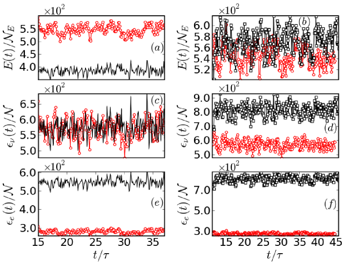
Figures 1(a)-(f) show the time evolution of the kinetic energy
, viscous energy-dissipation
rate , and
energy-dissipation rate because of the Ekman friction
(non-dimensionalized, respectively, by
and ).
The mean values , ,
and , given in
Table 1, are comparable to those in experiments; note that
and are of similar magnitudes. By comparing data
from runs (red circles) and (black lines) in
Figs. 1(a), (c), and (e) we see that, if we fix and
increase , decreases, remains unchanged (within error bars),
and increases. If we change both and , we can keep the
mean fixed, as in runs R1 and R3 in Table 1, by compensating
an increase in with an increase in (cf. Ref. riv01 );
in Figs. 1(b), (d), and (f) we see, by comparing runs R1 (red circles) and R3
(black squares), that remains unchanged (within error bars), whereas both
and increase as and increase in such a way
that is held fixed.
Figure 1: (Color online) Representatitve plots from runs (red circles),
(black lines), and (black squares), showing the time
evolution of [ and ],
[ and ], and
[ and ]. In ,
, and we keep fixed and vary
((red circles) and
(black line)). In , , and we
maintain by varying ((red
circles) and (black squares)) and .
Since Kolmogorov forcing is inhomogeneous, we use the
decomposition and , where the angular brackets
denote a time average and the prime the fluctuating part
111Experiments riv00 ; riv01 ; dan02 achieve
homogeneity via a periodic, square-wave forcing with amplitude
; this introduces another time-scale in the problem; to
avoid this complication we work with a time-indepedent force.,
to calculate the order- velocity and vorticity structure
functions
and ,
respectively, where has magnitude and is an origin.
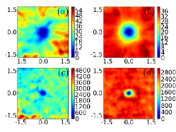
Figures 2(a) and (b) show pseudocolor plots of
and , respectively, for
; other values of yield similar results so
long as they do not lie near the boundary layer (Table 1) of thickness
( is chosen at least away from all boundaries).
We now calculate and
, where
the subscript denotes an average over the origin (we use ); these
averaged structure functions [Figs. 2(c) and (d)] are nearly isotropic
for but not so for . To obtain the isotropic parts in an
decomposition of these structure functions bou05 we integrate over the angle that
makes with the axis to obtain and
.
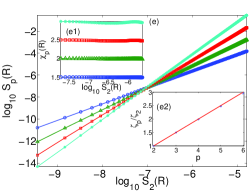
Given and we use the extended-self-similarity (ESS) procedure ben93 to extract
the multiscaling-exponent ratios and
, respectively, from
the slopes (in the forward-cascade inertial range) of log-log plots of
versus [Fig. 2(e)] and
versus [Fig. 2(f)] 222We employ ESS since
forward-cascade inertial ranges have a very modest extent even in the largest DNS studies tsa05 ; bof07
that use periodic domains and hyperviscosity.. The insets Figs. 2 (e1) and (f1) show,
respectively, plots of the local slopes versus
and versus
in the forward-cascade regime; the mean values of and , over the ranges shown,
yield the exponent ratios and that are plotted versus in
Figs. 2 (e2) and (f2), respectively, in which the error bars indicate the maximum deviations
of and from their mean values. The Kraichnan-Leith-Batchelor (KLB) predictions kraic67
for these exponent ratios, namely, and
, agree with our values for but not
: velocity structure functions do not display multiscaling [Fig. 2 (e2)]
whereas their vorticity analogs do [note the curvature of the plot in Fig. 2 (f2)].
This is in consonance with the results of DNS
studies with periodic boundary conditions tsa05 ; bof07 . Indeed, if we use the same values of
as in Ref. tsa05 , we obtain the same exponent ratios (within error bars); thus our method for the
extraction of the isotropic parts of the structure functions suppresses boundary and anisotropy effects efficiently.
Figure 2: (Color online) Pseudocolor plots of (a) , for
, (b) (average of
over ), (c) , for
, and (d) (average of
over ). Log-log ESS plots
of the isotropic parts of the order- (e) velocity structure
functions versus and (f) the vorticity
structure functions versus ;
(blue line with circles), (green line with triangles),
(red line with squares), and (cyan line with stars);
plots of the local slopes and (see text), in the
forward-cascade inertial range: (e1) versus and
(f1) versus .
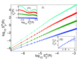
Plots versus of the exponent ratios (e2) ,
along with the KLB prediction (red line), and
(f2) and error bars from the
local slopes (see text). All plots are for run R7.
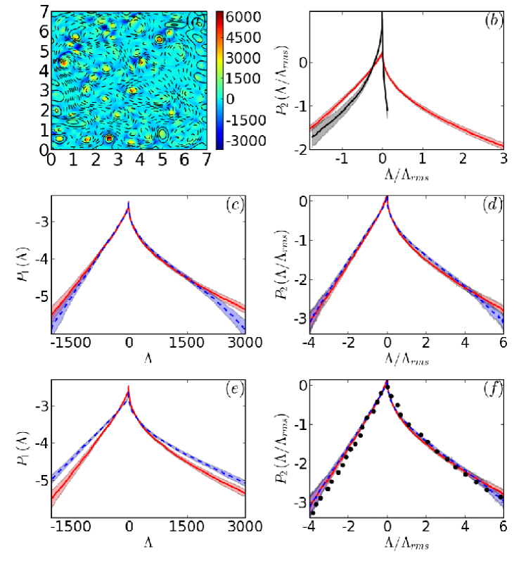
For an inviscid, incompressible 2D fluid the local flow topology
can be characterized via the Weiss criterion wei92 that
uses the invariant , where
and
. This
criterion provides a useful measure of flow properties even if
as noted in the experiments of Ref. riv01 :
Regions with and correspond to
centers and saddles as we show in Fig. 3 (a) by
superimposing, at a representative time, a pseudocolor plot of
on contours of . This result is in qualitative
accord with experiments [see, e.g., Fig. of
Ref. riv01 and also earlier DNS studies wei92 ,
which do not use Ekman friction]. In Fig. 3 (b) we
compare the scaled PDFs with data
obtained from points near the walls (black curve) and from points
in the bulk (red curve); the clear difference between these, not
highlighted before, indicates that regions of large
are suppressed in the boundary layers. There is a
generation of strain and vorticity in these boundary layers and
scatter plots, not shown, indicate
here; this leads to the suppression of regions of large
in .
Figure 3: (Color online) (a) Representative pseudocolor
plot of superimposed on a contour plot of the stream
function ; (b) the PDF obtained from points in
the bulk (red line) and from
those points within a distance from the boundaries
(black line) for our run ; plots of
(c) versus and (d)
versus for fixed and
(red line) and (blue dashed line)
[runs and ]; plots of (e)
versus and (f) versus
[runs and with
] and (red line) and
(blue dashed line) and points (black dots) extracted from
Fig. 2(d) of Ref. riv01 . In (c)-(f) the fluctuating part of the
velocity is used for . One-standard-deviation error bars
are indicated by the shaded regions.
Figures 3 (c) and (d) show the PDF
and the scaled PDF for runs (red line)
and (blue dashed line), with and ,
respectively, and ;
by comparing these figures we see that both and overlap
within error bars for runs and . We believe this
is because, in fixed- runs like and ,
does not change [Table 1] even though changes.
By contrast, if we compare and [Figs. 3 (e) and (f)]
for runs (red line) and (blue dashed line), in which
the mean is held fixed by tuning both and , we find, in agreement with
experiments riv01 , that the PDFs do not agree for
these runs, but the PDFs overlap within error bars. Our
results for in Fig. 3(f) are in quantitative
agreement with experiments: we have obtained the points in this
plot by digitising data points [see http://www.frantz.fi/software/g3data.php]
in Fig. 2(d) of Ref. riv01 ; the errors in
these points are comparable to the spread of data
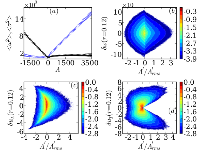
in riv01 . Conditional expectation values of
and , for a
given value of , also agree well with experiments as can
be seen by comparing Fig. 4 with Fig. of
Ref. riv01 . We also present in Figs. 4 (b-d)
pseudocolor plots of the joint PDFs of
, or with
, , , a circular disc with center at
and radius , and in the forward-cascade regime; we obtain striking
agreement with experiments as can be seen by comparing
Figs. 4 (c-d) with Figs. - of Ref. dan02 .
Finally, we calculate and
(see Table 1) and obtain excellent
agreement with experiments riv01 .
Figure 4:
(Color online)
(a) Plots of conditional expectation values, with one-standard-deviation
error bars, of (dots) and (circles)
for a given ; pseudocolor plots of (b) the joint PDF
,
(c) the joint PDF , and
(d) the joint PDF for
our run R7. The contours and the shading are for the logarithms
of the joint PDFs.
Some earlier numerical studies of 2D, wall-bounded, statistically
steady turbulent flows cle05 use forcing functions that are not of
the Kolmogorov type; furthermore, they do not include Ekman
friction. Other numerical studies, which include Ekman friction
and Kolmogorov forcing, employ periodic boundary
conditions ban08 ; bof07 ; tsa05 . To the best of our
knowledge our study of 2D turbulent flows is the first one
that accounts for Ekman friction, realistic boundary conditions,
and Kolmogorov forcing. Thus we can make quantitative comparisons
with soap-film experiments; and the agreement between our results
and those of Refs. riv00 ; riv01 ; dan02 ; riv07 vindicates the
use Eq. (1) as a model for these soap films cho01 .
We hope our results will stimulate experimental studies designed
to extract (a) the isotropic parts of structure functions (and thereby to
probe the multiscaling of vorticity structure
functions [Fig. 2 (f1)]) or (b) the
PDF [Fig. 3 (b)] near soap-film boundaries.
We thank J. Bec, G. Falkovich, V. Kumar, D. Mitra, and S.S. Ray for
discussions, CSIR, DST, and UGC(India) for financial support, and
SERC(IISc) for computational facilities. RP is a member of the
International Collaboration for Turbulence Research.
References
(1)
R. Kraichnan, Phys. Fluids 10, 1417 (1967);
C. Leith, Phys. Fluids, 11, 671 (1968);
G. Batchelor, Phys. Fluids Suppl. II 12, 233 (1969).
(2)
U. Frisch, Turbulence the legacy of A.N. Kolmogorov (Cambridge University
Press, Cambridge, 1996).
(3)
G. Boer and T. Shepherd, J. Atmos. Sci. 40, 164 (1983).
(4)
S. Danilov and D. Gurarie, Phys.–Usp. 43, 863 (2000);
H. Kellay and W. Goldburg, Rep. Prog. Phys. 65, 845 (2002);
P. Tabeling, Phys. Rep. 362, 1 (2002).
(5)
M. Rivera and X.L. Wu, Phy. Rev. Lett. 85, 976 (2000).
(6)
M. Rivera, X.L. Wu, and C. Yeung, Phys. Rev. Lett. 87, 044501 (2001).
(7)
W.B. Daniel and M.A. Rutgers, Phys. Rev. Lett. 89, 134502 (2002).
(8)
M. Rivera and R. Ecke, arXiv:0710.5888v1 (2007).
(9)
E. Bouchbinder, I. Procaccia, and S. Sela, Phys. Rev. Lett. 95, 255503
(2005).
(10)
R. Benzi et al., Phys. Rev. E 48, R29 (1993).
(11)
J. Weiss, Physica D 48, 273 (1992);
A. Provenzale and A. Babiano, J. Fluid Mech. 257, 533 (1993).
(12)
J. Chomaz, J. Fluid Mech. 442, 387 (2001).
(13)
C. Doering and J. Gibbon, pp. 23-24, Applied Analysis of the Navier-Stokes equations
(Cambridge University Press, Cambridge, 1995).
(14)
W. Press, B. Flannery, S. Teukolsky, and W. Vetterling, pp. 848-852, Numerical Recipes
in Fortran (Cambridge University Press, Cambridge, 1992).
(15)
W. E and J.-G. Liu, J. Comp. Phys. 124, 368 (1996).
(16)
H. Clercx, G. Heijst, D. Molenaar, and M. Wells, Dyn. Atmos. Oceans 40, 3 (2005);
G.J.F. van Heijst, H.J.H Clercx, and D. Molenaar, J. Fluid. Mech. 554, 411 (2006).
(17)
Y.-K. Tsang, E. Ott, T.M. Antonsen, and P.N. Guzdar, Phys. Rev. E 71, 066313
(2005).
(18)
G. Boffetta, J. Fluid Mech. 589, 253 (2007).
(19)
M.M. Bandi and C. Connaughton, Phys. Rev. E 77, 036318 (2008).