Virtual Reshaping and Invisibility in Obstacle Scattering

Abstract

We consider reshaping an obstacle virtually by using transformation optics in acoustic and electromagnetic scattering. Among the general virtual reshaping results, the virtual minification and virtual magnification are particularly studied. Stability estimates are derived for scattering amplitude in terms of the diameter of a small obstacle, which implies that the limiting case for minification corresponds to a perfect cloaking, i.e., the obstacle is invisible to detection.

1 Introduction

Since the pioneering work on transformation optics and cloaking [9, 10, 13, 24], there is an avalanche of study on designs of various striking cloaking devices; e.g., invisibility cloaking devices [6, 12]; field rotators [1]; concentrators [17]; electromagnetic wormholes [4, 5]; superscatterers [25], etc.. We refer to a most recent survey paper [7] for a comprehensive review and related literature. The crucial observation is that certain PDEs governing the wave phenomena are form-invariant under transformations, e.g., Hemholtz equation for acoustic scattering and Maxwell’s equations for electromagnetic scattering. Hence, one could form new acoustic or EM material parameters (in the physical space) by pushing forward old ones (in the virtual space) via a mapping $F$. Such materials/media are called transformation media [24]. It turns out that the wave solutions in the virtual space with the old material parameters and in the physical space with the new material parameters are also related by the push-forward $F$. Those key ingredients pave the way for the design of optical devices with customized effects on wave propagation.

In this paper, we shall be concerned with cloaking devices for acoustic and electromagnetic obstacle scattering. As is known, there are two types of scatterers which are under wide study for acoustic and electromagnetic scattering, namely, the penetrable medium and the impenetrable obstacle. For a medium, the acoustic or EM wave can penetrate inside, and basically the medium accounts for the coefficients in the governing PDEs. Whereas for an obstacle, the acoustic or EM wave cannot penetrate inside and only exists in the exterior of the object, and the obstacle is related to the domain of definitions for the governing PDEs. The cloakings for acoustic or EM media have been extensively studied in transformation optics in existing literature and the theory has been well-established, we again refer to the review paper [7] for related discussion. For our current study, the cloakings for obstacles are considered and it is shown that the domain of definitions for certain PDEs can also be pushed forward under transformations. Using the transformation optics, one can push forward an obstacle in the virtual space to form a different obstacle in the physical space, and the ambient space around the virtual obstacle is then pushed forward to a cloaking medium around the physical obstacle. With a suitable push-forward $F$, it is shown that the scattering amplitude in the physical space coincides with that in the virtual space. That is, if one intends to recover the physical obstacle after being cloaked by the corresponding scattering measurements, then the reconstruction will give the image of the obstacle in the virtual space, but not the physical one, namely, the physical obstacle is virtually reshaped with the cloaking. Principally, it has been shown that one can achieve any desired virtual reshaping effect provided an appropriate transformation $F$ can be found between the virtual space and the physical space.

Particularly, we consider virtually magnifying and minifying an obstacle. By magnification, we mean that the size of the virtual obstacle is larger than that of the underlying physical one. That is, under acoustic and EM wave detection, the cloaking makes the obstacle look bigger than its original size. Whereas by minification, we actually mean virtually shrinking the obstacle, that is, the size of the virtual obstacle is smaller than that of the physical one. In the limiting case of minification, the virtual obstacle collapses to a single point, and this formally corresponds to a perfect cloaking, namely, the physical obstacle becomes invisible to detection. We note that in this case, the push-forward $F$ blows up a single point in the virtual space to a ‘hole’ (which actually is the physical obstacle) in the physical space. Hence, the map $F$ is intrinsically singular, and the obtained transformation medium is inevitably singular. Correspondingly, the transformed PDEs in the physical space are no longer uniformly elliptic which also becomes singular. Therefore, in order to rigorously justify the perfect cloaking, we need to deal with the singular PDEs. Basically, one would encounter the same problems in treating perfect cloakings for acoustic or EM medium and several approaches are proposed to deal with such singularities. For perfect cloaking of conductivity equation, which can be considered as optics at zero frequency, the invisibility is mathematically justified in [10] by using the removability of point singularities for harmonic functions; whereas an alternative treating is provided in [12], where near-invisibility is introduced from a regularization viewpoint and the invisibility is rigorously justified based on certain stability estimates for conductivity equation with small inclusions. For the finite frequency cases, a novel notion of finite energy solutions is introduced in [8] and the invisibility cloaking of acoustic and electromagnetic medium are then justified directly. For the perfect cloaking of obstacles considered in the present paper, we shall follow the approach in [12] to mathematically justify the invisibility by taking limit of near-invisibility. To that end, we derive certain stability estimates for scattering amplitudes in terms of the diameter of a small obstacle in both acoustic and EM scattering. Those stability estimates are then used to show that the limiting process of minification cloaking corresponds to a process of near-invisibility cloaking, which in turn implies the desired invisibility result of the perfect cloaking. For practical considerations, all our reshaping studies are conducted within multiple scattering, that is, there is more than one obstacle component included.

Finally, we would like to mention some unique determination results in inverse obstacle scattering, where one utilizes acoustic or electromagnetic scattering measurements to identify an unknown/inaccessible obstacle. The uniqueness/identifiability results correspond to circumstances under which one cannot virtually reshape an obstacle. In the case that the obstacle is situated in a homogeneous background medium, the uniqueness theory for inverse obstacle scattering is relatively well established, and we refer to [16] for a survey and relevant literature. Whereas in [11],[15],[22], the recovery of an obstacle included in certain inhomogeneous (isotropic) medium is considered. It is shown in [11] and [22] that if the isotropic medium is known a priori, then the included obstacle is uniquely determined by the associated scattering amplitude. Under the assumption that the isotropic medium and the included obstacle has only planar contacts, it is proved in [15] that one can recover both the medium and the obstacle by the associated scattering amplitude. The argument in [15] also implies that an obstacle surrounded by an isotropic medium cannot produce the same scattering amplitude as another pure obstacle. This result essentially indicate that transformation media for virtually reshaping an obstacle must be anisotropic.

The rest of the paper is organized as follows. In Section 2, we consider the reshaping for acoustic scattering, where virtual minification and magnification are first considered consecutively, and then we present a general reshaping result. Similar study has been conducted for reshaping a EM perfectly conducting obstacle in Section 3.

2 Virtual reshaping for acoustic scattering

2.1 The Helmholtz equation

Let $M$ be an open subset of $\mathbb{R}^{3}$ with Lipschitz continuous boundary $\partial M$ and connected complement $M^{+}:=\mathbb{R}^{3}\backslash\overline{M}$. Let $(M^{+},g)$ be a Riemannian manifold such that $g$ is Euclidean outside of a sufficiently large ball $B_{R}$ containing $M$. Here and in the following, $B_{R}$ shall denote an Euclidean ball centered at origin and of radius $R$. In wave scattering, $M$ denotes an impenetrable obstacle and the Remannian metric $g$ corresponds to the surrounding medium with the Euclidean metric $g_{0}:=\delta_{i}^{j}$ representing the vacuum. In acoustic scattering, $\sigma=(\sigma^{ij})_{i,j=1}^{3}$ with $\sigma^{ij}:=\sqrt{|g|}g^{ij}$ is the anisotropic acoustic density and $\sqrt{|g|}=|\sigma|$ is the bulk modulus, where $(g^{ij})_{i,j=1}^{3}$ is the matrix inverse of the matrix $(g_{ij})_{i,j=1}^{3}$, and $|g|=\det g,|\sigma|=\det\sigma$. Formally, we have the following one-to-one correspondence between a material parameter tensor and a Riemannian metric

$$\sigma^{ij}=|g|^{1/2}g^{ij}\quad\mbox{or}\quad g^{ij}=|\sigma|^{-1}\sigma^{ij}.$$ (2.1)

We consider the scattering for a time-harmonic plane incident wave $u^{i}=\exp\{ikx\cdot\theta\}$, $\theta\in\mathbb{S}^{2}$ due to the obstacle $M$ together with the surrounding medium $(M^{+},g)$. The total wave field is governed by the Helmholtz equation

$$\Delta_{g}u+k^{2}u=0\quad\mbox{in $M^{+}$},$$ (2.2)

$$u|_{\partial M}=0,$$ (2.3)

where the Laplace-Beltrami operator associated with $g$ is given in local coordinates by

$$\Delta_{g}u=\frac{1}{\sqrt{g}}\sum_{i,j=1}^{3}\frac{\partial}{\partial x_{i}}\left(\sqrt{|g|}g^{ij}\frac{\partial u}{\partial x_{j}}\right).$$

The homogeneous Dirichlet boundary condition (2.3) means that the wave pressure vanishes on the boundary of the obstacle. $M$ is usually referred to as a sound-soft obstacle. The scattered wave field is as usual assumed to satisfy the Sommerfeld radiation condition. Taking advantage of the one-to-one correspondence (2.1) between (positive definite) acoustic densities $\sigma$ and Riemannian metrics $g$, we proceed to mention a few facts about the form-invariance of the Hemholtz equation under transformations. For a smooth diffeomorphism $F:=\Omega_{1}\rightarrow\Omega_{2}$, $y=F(x)$, the metric $g(x)$ transforms as a covariant symmetric 2-tensor,

$$\tilde{g}_{ij}(y):=(F_{*}g)_{ij}(y)=\sum_{l,m=1}^{3}\frac{\partial x^{l}}{\partial y^{i}}\frac{\partial x^{m}}{\partial y^{j}}g_{lm}\bigg{|}_{x=F^{-1}(y)},$$ (2.4)

and then, for $u=\tilde{u}\circ F$, we have

$$(\Delta_{g}+k^{2})u=0\Longleftrightarrow(\Delta_{\tilde{g}}+k^{2})\tilde{u}=0.$$ (2.5)

Alternatively, using (2.1), one could work with the Helmholtz equation of the following form

$$\sum_{i,j=1}^{3}\partial_{i}(\sigma^{ij}\partial_{j}u)+k^{2}|\sigma|u=0,$$ (2.6)

and then, for $u=\tilde{u}\circ F$, we have

$$\sum_{i,j=1}^{3}\partial_{i}({\tilde{\sigma}}^{ij}\partial_{j}u)+k^{2}|\tilde{\sigma}|u=0.$$ (2.7)

Here $\tilde{\sigma}$ is the push-forward of $\sigma$ which, by using (2.1) and (2.4), can be readily shown to be given by

$$\tilde{\sigma}=F_{*}\sigma:=\left(\frac{(DF)^{T}\cdot\sigma\cdot(DF)}{|\det DF|}\right)\circ F^{-1},$$ (2.8)

where $DF$ denotes the (matrix) differential of $F$ and $(DF)^{T}$ its transpose.

Throughout, we shall work with $\sigma\in L^{\infty}(M^{+})^{3\times 3}$ and $F$ is orientation-preserving, invertible with both $F$ and $F^{-1}$ (uniformly) Lipschitz continuous over $M^{+}$. So, it is appropriate to work with the following Sobolev space for the scattering solution to (2.2)-(2.3),

$$H_{loc}^{1}(M^{+})=\{u\in\mathscr{D}^{\prime}(M^{+});u\in H^{1}(M^{+}\cap B_{\rho})\ \ \mbox{for each finite $\rho$ with $M\subset B_{\rho}$}\}.$$

The system (2.2)-(2.3), or (2.6) and (2.3) is well-posed and has a unique solution $u\in H_{loc}^{1}(M^{+})$ (see [19]). Noting that the corresponding metric outside a ball $B_{R}\supset M$ is Euclidean, we know $u$ is smooth outside $B_{R}$. Furthermore, the solution $u(x,k,\theta)$ admits asymptotically as $|x|\rightarrow+\infty$ the development (see [3])

$$u(x,\theta,k)=e^{ikx\cdot\theta}+\frac{e^{ik|x|}}{|x|}A(\theta^{\prime},\theta,k)+\mathcal{O}(\frac{1}{|x|^{2}}),$$ (2.9)

where $\theta^{\prime}=x/|x|\in\mathbb{S}^{2}$. The analytic function $A(\theta^{\prime},\theta,k)$ is known as the scattering amplitude or far-field pattern. According to the celebrated Rellich’s theorem, there is a one-to-one correspondence between the scattering amplitude $A(\theta^{\prime},\theta,k)$ and the wave solution $u(x,\theta,k)$. Throughout, we consider the scattering amplitude for the virtual reshaping effects.

We shall denote by $M\bigoplus(M^{+},g)$ a cloaking device with an obstacle $M$ and the corresponding cloaking medium $(M^{+},g)$. The metric $g$ is always assumed to be Euclidean outside a sufficiently large ball containing $M$, namely, the cloaking medium is compactly supported. If we know the support of the cloaking medium, say $M^{\prime}\backslash\overline{M}$, we also write $M\bigoplus(M^{\prime}\backslash\overline{M},g)$ to denote the cloaking device.

Definition 2.1.

We say that $M\bigoplus(M^{+},g)$ (virtually) reshapes the obstacle $M$ to another obstacle $\widetilde{M}$, if the scattering amplitudes coincide for $M\bigoplus(M^{+},g)$ and $\widetilde{M}$, i.e.

$$A(\theta^{\prime},\theta,k;M\bigoplus(M^{+},g))=A(\theta^{\prime},\theta,k;\widetilde{M}).$$

We would like to remark that according to the correspondence (2.1), the cloaking device in Definition (2.1) can also be written as $M\bigoplus(M^{+},\sigma)$, where $\sigma$ is the (anisotropic) acoustic density for the cloaking medium.

2.2 Virtual minification by cloaking

We first consider the reshaping effects for a special class of obstacles, which are star-shaped and referred to as $l^{p}$-ball shaped obstacles in the following. They are domains in $\mathbb{R}^{3}$ of the form

$$\{x\in\mathbb{R}^{3};\|x\|_{p}=r\},$$

where $p\in[1,+\infty]$, $r>0$ is a constant and for $x=(x_{1},x_{2},x_{3})$

$$\|x\|_{p}=\left(\sum_{i=1}^{3}|x_{i}|^{p}\right)^{1/p}.$$

Obviously, $\|\cdot\|_{2}=|\cdot|$ and an $l^{2}$-ball is exactly an Euclidean ball. For $l^{p}$-ball shaped obstacles, we can give the transformation rule explicitly and correspondingly, the cloaking material parameters for those obstacles can be derived explicitly. Henceforth, we write $B_{R,p}$ to denote an $l^{p}$-ball of radius $R$ and centered at origin, whereas as prescribed earlier, we write $B_{R}:=B_{R,2}$. We also denote by $M^{+}$ the complement of a domain $M$ in $\mathbb{R}^{3}$.

Let $M=B_{R_{1},p}$ with $R_{1}>0$. Let $R_{0},R_{2}$ be such that $0<R_{0}<R_{1}<R_{2}$. We define the map, $F:B_{R_{0},p}^{+}\mapsto B_{R_{1},p}^{+}$ by

$$x:=F(y)=\begin{cases}\qquad y,\ &\mbox{for $\|y\|_{p}\geq R_{2}$},\\ (\frac{R_{1}-R_{0}}{R_{2}-R_{0}}R_{2}+\frac{R_{2}-R_{1}}{R_{2}-R_{0}}\|y\|_{p})\frac{y}{\|y\|_{p}},\ \ &\mbox{for $R_{0}<\|y\|_{p}<R_{2}$}.\end{cases}$$ (2.10)

It is noted that $F$ is (uniformly) Lipschitz continuous over $B_{R_{0},p}^{+}$ and maps $B_{R_{2},p}\backslash B_{R_{0},p}$ to $B_{R_{2},p}\backslash B_{R_{1},p}$. For $R_{1}<\|x\|_{p}<R_{2}$, let

$$g_{1}(x)=(F_{*}g_{0})(x).$$ (2.11)

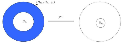
Figure 1: Illustration for minification: the cloaking device $B_{R_{1}}\bigoplus(B_{R_{1}}^{+},g)$ virtually reshapes $B_{R_{1}}$ to $B_{R_{0}}$.

Set

$$g(x)=\begin{cases}g_{1}(x),\ &\mbox{for $R_{1}<\|x\|_{p}<R_{2}$},\\ g_{0}(x),&\mbox{for $\|x\|_{p}\geq R_{2}$}.\end{cases}$$ (2.12)

We have

Proposition 2.2.

The cloaking device $B_{R_{1},p}\bigoplus(B_{R_{1},p}^{+},g)$ with $g$ defined in (2.12), reshapes $B_{R_{1},p}$ virtually to $B_{R_{0},p}$. That is, the physical obstacle $B_{R_{1},p}$ with the cloaking material $(B_{R_{2},p}\backslash B_{R_{1},p},g_{1})$ is virtually minified to the obstacle $B_{R_{0},p}$ with a minification ratio $\kappa:=R_{0}/R_{1}$ (see Fig. 1 for a schematic illustration).

Proof.

Let $u(y)\in H_{loc}^{1}(B_{R_{0},p}^{+})$ be the unique solution to the Hemholtz equation (2.2)-(2.3) corresponding to the obstacle $B_{R_{0},p}$. Whereas, we let $v(x)\in H_{loc}^{1}(B_{R_{1},p}^{+})$ be the unique solution to the Helmholtz equation (2.2)-(2.3) corresponding to $B_{R_{1},p}\bigoplus(B_{R_{1},p}^{+},$ $g)$. Define $\tilde{u}(x),x\in B_{R_{1},p}^{+},$ be such that $u=\tilde{u}\circ F$, i.e. $\tilde{u}=F_{*}u=(F^{-1})^{*}u$. It is clear that $\tilde{u}\in H_{loc}^{1}(B_{R_{1},p}^{+})$ since $F$ is bijective and both $F$ and $F^{-1}$ are (uniformly) Lipschitz continuous. Moreover, noting $F(\partial B_{R_{0},p})=\partial B_{R_{1},p}$, we know $\tilde{u}|_{\partial B_{R_{1},p}}=0$.

By the invariance of Helmholtz equation under transformation, it is readily seen that $\tilde{u}=v$. Hence,

$$A(\theta^{\prime},\theta,k;B_{R_{1},p}\bigoplus(B_{R_{1},p}^{+},g))=A(\theta^{\prime},\theta,k;B_{R_{0},p}).$$ (2.13)

∎

For an Euclidean ball $B_{R_{0}}\subset\mathbb{R}^{3}$, by separation of variables, we have

$$A(\theta^{\prime},\theta,k;B_{R_{0}})=\frac{i}{k}\sum_{n=0}^{\infty}(2n+1)\frac{j_{n}(kR_{0})}{h_{n}^{(1)}(kR_{0})}P_{n}(\cos\psi),$$ (2.14)

where $j_{n}(t)$ and $h_{n}^{(1)}(t)$ are respectively, the $n$-th order spherical Bessel function and spherical Hankel function of first kind, $P_{n}(t)$ is the Legendre polynomial and $\psi=\angle(\theta,\theta^{\prime})$. Using the asymptotical properties

$$j_{n}(t)=\mathcal{O}(t^{n}),\ \ h_{n}^{(1)}(t)=\mathcal{O}(t^{-n-1}),\ \ n=0,1,\ldots,\ \ \mbox{as\ $t\rightarrow+0$},$$

it is straightforward to show

$$A(\theta^{\prime},\theta,k;B_{R_{0}})=\mathcal{O}(R_{0})\quad\mbox{as $R_{0}\rightarrow+0$,}$$ (2.15)

Now we consider the limiting case for minification, namely $\kappa\rightarrow+0$ or equivalently $R_{0}\rightarrow+0$. By (2.13) and (2.15),

$$A(\theta^{\prime},\theta,k;B_{R_{1}}\bigoplus(B_{R_{1}}^{+},{g}))=A(\theta^{\prime},\theta,k;B_{R_{0}})=\mathcal{O}(R_{0})$$ (2.16)

as $R_{0}\rightarrow+0$. That is,

Proposition 2.3.

The limit for minification of an Euclidean ball $B_{R_{1}}$ in Proposition 2.2 gives a perfect cloaking, namely, it makes the obstacle invisible to detection.

In the limiting case with $\kappa=0$, the transformation in (2.10) becomes

$$x=H(y):=\begin{cases}\quad y,\quad\mbox{for $\|y\|_{p}\geq R_{2}$},\\ (R_{1}+\frac{R_{2}-R_{1}}{R_{2}}\|y\|)\frac{y}{\|y\|_{p}},&\mbox{for $0<\|y\|_{p}<R_{2}$},\end{cases}$$ (2.17)

which maps $\mathbb{R}^{3}\backslash\{0\}$ to $\mathbb{R}^{3}\backslash B_{R_{1},p}$, i.e., it blows up the single point $\{0\}$ to $B_{R_{1},p}$. It is remarked that the map $H$ in (2.17) with $p=2$ is exactly the one used in [9, 10] for perfect cloaking of conductivity equation, and in [24] for perfect cloaking of electromagnetic material tensors. Next, we take the case with $p=2$ as an example for a simple analysis of the perfect cloaking medium. The corresponding metric $(H_{*}g_{0})(x)$ in $B_{R_{2}}\backslash\bar{B}_{R_{1}}$ is singular near the cloaking interface, namely $\partial B_{R_{1}}$. In fact, considering in the standard spherical coordinates on $B_{R_{2}}\backslash\{0\}$, $(r,\phi,\theta)\mapsto(r\sin\theta\cos\phi,r\sin\theta\sin\phi,r\cos\theta)\in\mathbb{R}^{3}$ and by (2.4), it can be easily calculated that

$$\tilde{g}:=H_{*}g_{0}=\left(\begin{array}[]{ccc}\lambda^{2}&0&0\\ 0&\lambda^{2}(r-R_{1})^{2}&0\\ 0&0&\lambda^{2}(r-R_{1})^{2}\sin^{2}\theta\\ \end{array}\right),$$

where $\lambda=R_{2}/(R_{2}-R_{1})$. That is, $\tilde{g}$ has one eigenvalue bounded from below (with eigenvector corresponding to the radial direction) and two eigenvalues of order $(r-R_{1})^{2}$ approaching zero as $r\rightarrow+R_{1}$. Hence, if the perfect cloaking is analyzed directly, one needs to deal with the degenerated elliptic equation near the cloaking interface. So, a suitable choice of the class of weak solutions to the singular equation must be purposely introduced, as the finite energy solutions considered in [8] for invisibility cloaking devices of acoustic and electromagnetic media. Clearly, our earlier analysis on the perfect cloaking of an Euclidean ball avoid singular equation by taking limit. This is similar to [12] for the analysis of perfect cloaking of conductivities in electrical impedance tomography by regularization. Here we would like to point out that there is no theoretical result available showing that the limit of the regularized solutions obtained by the approach of the current paper by sending $\kappa\rightarrow 0$ are the finite energy solutions in the sense of [8]. A further study in this aspect may provide more insights into the invisibility cloaking.

In order to achieve the similar invisibility result for a general $l^{p}$-ball shaped obstacles, we need to derive stability estimates similar to (2.16) for generally shaped obstacles with small diameters. This is given by Lemma 2.4 below, proved using boundary integral representation rather than separation of variables, and the obstacles could be generally star-shaped. On the other hand, from a practical viewpoint, we consider the scattering with multiple scattering components and only some of the components are cloaked. We shall show that the virtual reshaping takes effect only for those cloaked components and the other uncloaked components remain unaffected. Particularly, those perfectly cloaked components will be invisible, even though there is scattering interaction between the obstacle components. We are now in a position to present the key lemma. In the sequel, we let $\mathbb{B}$ be a simply connected set in $\mathbb{R}^{3}$ whose boundary is star-shaped with respect to the origin of the form $\partial\mathbb{B}=\delta r_{0}(\theta)\theta$, where $\theta\in\mathbb{S}^{2},r_{0}(\theta)\in C^{2}(\mathbb{S}^{2})$ and $\delta>0$. Let $\mathbb{B}_{0}$ be the domain $\{x\in\mathbb{R}^{3};|x|<r_{0}(\theta)\}$.

Lemma 2.4.

Suppose $M_{1}\cap\mathbb{B}_{0}=\emptyset$, then we have

$$A(\theta^{\prime},\theta,k;M_{1}\cup\mathbb{B})=A(\theta^{\prime},\theta,k;M_{1})+\mathcal{O}(\delta)\quad\mbox{as $\delta\rightarrow+0$}.$$ (2.18)

Proof.

Let $\Phi(x,y)=e^{ik|x-y|}/(4\pi|x-y|)$ be the fundamental solution to the Helmholtz operator $(\Delta+k^{2})$. We know that $u(x;k,\theta)\in C^{2}(\mathbb{R}^{3}\backslash\overline{M_{1}\cup\mathbb{B}})\cap C(\mathbb{R}^{3}\backslash(M_{1}\cup\mathbb{B}))$ and can be represented in the form (see [3])

$$\begin{split}u(x;M_{1}\cup\mathbb{B})=e^{ikx\cdot\theta}+&\int_{\partial M_{1}}\bigg{\{}\frac{\partial\Phi(x,y)}{\partial\nu(y)}-{i}\Phi(x,y)\bigg{\}}\varphi_{1}(y)\ ds(y)\\ +&\int_{\partial\mathbb{B}}\bigg{\{}\frac{\partial\Phi(x,y)}{\partial\nu(y)}-{i\eta}\Phi(x,y)\bigg{\}}\varphi_{2}(y)\ ds(y),\end{split}$$ (2.19)

where $\varphi_{1}\in C(\partial M_{1})$ and $\varphi_{2}\in C(\partial\mathbb{B})$ are density functions, and $\eta\neq 0$ is a real coupling parameter. The densities $\varphi_{1}$ and $\varphi_{2}$ are unique solutions to the following integral equation (see [3])

$$\begin{split}\varphi(x)+&2\int_{\partial M_{1}}\bigg{\{}\frac{\partial\Phi(x,y)}{\partial\nu(y)}-{i}\Phi(x,y)\bigg{\}}\varphi_{1}(y)\ ds(y)\\ +&2\int_{\partial\mathbb{B}}\bigg{\{}\frac{\partial\Phi(x,y)}{\partial\nu(y)}-{i\eta}\Phi(x,y)\bigg{\}}\varphi_{2}(y)\ ds(y)=-2e^{ikx\cdot\theta},\end{split}$$ (2.20)

for $x\in\partial M_{1}\cup\partial\mathbb{B}$, where $\varphi(x):=\varphi_{1}(x)$ for $x\in\partial M_{1}$ and $\varphi(x):=\varphi_{2}(x)$ for $x\in\partial\mathbb{B}$. We introduce the integral operators

$$(S_{1}\varphi_{1})(x)=2\int_{\partial M_{1}}\Phi(x,y)\varphi_{1}(y)ds(y),\quad(K_{1}\varphi_{1})(x)=2\int_{\partial M_{1}}\frac{\partial\Phi(x,y)}{\partial\nu(y)}\varphi_{1}(y)ds(y)$$

$$(S_{2}\varphi_{2})(x)=2\int_{\partial\mathbb{B}}\Phi(x,y)\varphi_{2}(y)ds(y),\quad(K_{2}\varphi_{2})(x)=2\int_{\partial\mathbb{B}}\frac{\partial\Phi(x,y)}{\partial\nu(y)}\varphi_{2}(y)ds(y),$$

and set

$$h_{1}(x):=-2e^{ikx\cdot\theta},\ \ x\in\partial M_{1};\qquad h_{2}(x):=-2e^{ikx\cdot\theta},\ \ x\in\partial\mathbb{B}.$$

Then equation (2.20) can be rewritten as

$$[\varphi_{1}+K_{1}\varphi_{1}-{i}S_{1}\varphi_{1}+K_{2}\varphi_{2}-{i}\eta S_{2}\varphi_{2}](x)=h_{1}(x),\quad x\in\partial M_{1}$$ (2.21)

$$[\varphi_{2}+K_{2}\varphi_{2}-{i\eta}S_{2}\varphi_{2}+K_{1}\varphi_{1}-{i}S_{1}\varphi_{1}](x)=h_{2}(x),\quad x\in\partial\mathbb{B}.$$ (2.22)

It is remarked that the integral operators involved in equations (2.21) and (2.22) with weakly singular integral kernels have to be understood in the sense of Cauchy principle values and we refer to [3] and [19] for related mapping properties. Clearly, $\varphi_{1}$ and $\varphi_{2}$ are functions dependent on $\delta$. We next study their asymptotic behaviors as $\delta\rightarrow+0$. To this end, we fix $\delta>0$ but being sufficiently small and take $\eta=\delta^{-1}$.

In the sequel, without loss of generality, we may assume that $dist(\partial M_{1},\partial\mathbb{B}_{0})>c_{0}>0$, otherwise one can shrink $\mathbb{B}_{0}$ to $1/2\mathbb{B}_{0}$. By straightforward calculations, it can be easily shown that

$$\|K_{2}-{i\eta}S_{2}\|_{C(\partial\mathbb{B})\rightarrow C(\partial M_{1})}=\mathcal{O}(\delta),\ \|K_{1}-{i}S_{1}\|_{C(\partial M_{1})\rightarrow C(\partial\mathbb{B})}=\mathcal{O}(1).$$ (2.23)

Next, for $x\in\partial\mathbb{B}_{0}$, we define

$$(K_{0}\phi)(x)=2\int_{\partial\mathbb{B}_{0}}\frac{\partial\Phi_{0}(x,y)}{\partial\nu(y)}\phi(y)\ ds(y),\ (S_{0}\phi)(x)=2\int_{\partial\mathbb{B}_{0}}\Phi_{0}(x,y)\phi(y)\ ds(y),$$

where $\phi\in C(\partial\mathbb{B}_{0})$ and $\Phi_{0}(x,y)=1/(4\pi|x-y|)$ is the fundamental solution to the Laplace operator. It is known that both $S_{0}$ and $K_{0}$ are compact operators in $C(\partial\mathbb{B}_{0})$ (see [2]). By changing the integration to the boundary of the reference obstacle $\partial\mathbb{B}_{0}$, we have

$$(S_{2}\varphi)(x)= 2\int_{\partial\mathbb{B}}\frac{e^{ik|x-y|}}{|x-y|}\varphi(y)\ ds(y)=2\delta\int_{\partial\mathbb{B}_{0}}\frac{e^{ik\delta|x^{\prime}-y^{\prime}|}}{|x^{\prime}-y^{\prime}|}\varphi(\delta y^{\prime})\ ds(y^{\prime}),$$

$$(K_{2}\varphi)(x)= 2\int_{\partial\mathbb{B}}\partial\left(\frac{e^{ik|x-y|}}{|x-y|}\right)/\partial\nu(y)\varphi(y)\ ds(y)$$

$$= 2\int_{\partial\mathbb{B}_{0}}\partial\left(\frac{e^{ik\delta|x^{\prime}-y^{\prime}|}}{|x^{\prime}-y^{\prime}|}\right)/\partial\nu(y^{\prime})\varphi(\delta y^{\prime})\ ds(y^{\prime}),$$

where $\varphi\in C(\partial\mathbb{B})$, $x,y\in\partial\mathbb{B}$ and $x^{\prime}:=x/\delta,y^{\prime}=y/\delta\in\partial\mathbb{B}_{0}$. Then by using power series expansion of the exponential function $e^{ik\delta|x-y|}$, we have by direct calculations

$$\|\frac{1}{\delta}S_{2}-S_{0}\|_{C(\delta\partial\mathbb{B}_{0})\rightarrow C(\partial\mathbb{B}_{0})}=\mathcal{O}(\delta),\quad\|K_{2}-K_{0}\|_{C(\delta\partial\mathbb{B}_{0})\rightarrow C(\partial\mathbb{B}_{0})}=\mathcal{O}(\delta^{2}).$$ (2.24)

By changing the integration to $\partial\mathbb{B}_{0}$ and using the results in (2.24), we have from (2.22) that

$$\varphi_{2}(\delta x)=[I+K_{0}-iS_{0}+\mathcal{O}(\delta)]^{-1}[h_{2}(\delta x)-(K_{1}-{i}S_{1})\varphi_{1}(\delta{x})],\quad{x}\in\partial\mathbb{B}_{0}.$$ (2.25)

It is noted here that $(I+K_{0}-iS_{0})$ is bounded invertible (see [2]). Then, plugging (2.25) into (2.21) and using the relations in (2.23), we further have

$$\varphi_{1}=[I+K_{1}-\mathrm{i}S_{1}+\mathcal{O}(\delta)]^{-1}(h_{1}+\mathcal{O}(\delta)),$$ (2.26)

which, by noting $I+K_{1}-\mathrm{i}S_{1}$ is invertible (see [3]), gives

$$\varphi_{1}=\tilde{\varphi}_{1}+\mathcal{O}(\delta),$$ (2.27)

where

$$\tilde{\varphi}_{1}=[I+K_{1}-\mathrm{i}S_{1}]^{-1}h_{1}.$$

Furthermore, (2.27) together with (2.25) implies that

$$\varphi_{2}=\mathcal{O}(1).$$ (2.28)

Finally, by (2.19) we know

$$\begin{split}A(\theta^{\prime},\theta,k;M_{1}\cup\mathbb{B})=&\frac{1}{4\pi}\int_{\partial M_{1}}\bigg{\{}\frac{\partial e^{-iky\cdot\theta^{\prime}}}{\partial\nu(y)}-{i}e^{-iky\cdot\theta^{\prime}}\bigg{\}}\varphi_{1}(y)\ ds(y)\\ +&\frac{1}{4\pi}\int_{\partial\mathbb{B}}\bigg{\{}\frac{\partial e^{-iky\cdot\theta^{\prime}}}{\partial\nu(y)}-{i\eta}e^{-iky\cdot\theta^{\prime}}\bigg{\}}\varphi_{2}(y)\ ds(y).\end{split}$$ (2.29)

Using the estimates in (2.27) and (2.28) to (2.29) and changing the integration over $\partial\mathbb{B}$ to $\partial\mathbb{B}_{0}$, we have

$$A(\theta^{\prime},\theta,k;M_{1}\cup\mathbb{B})=A(\theta^{\prime},\theta,k;M_{1})+\mathcal{O}(\delta),$$

where we have made use of the fact that

$$A(\theta^{\prime},\theta,k;M_{1})=\frac{1}{4\pi}\int_{\partial M_{1}}\tilde{\varphi}_{1}(y)\bigg{\{}\frac{\partial e^{-{i}k\theta^{\prime}\cdot y}}{\partial\nu(y)}-{i}e^{-{i}k\theta^{\prime}\cdot y}\bigg{\}}\ ds(y).$$

The proof is completed. ∎

Remark 2.5.

If $\partial M_{1}\cup\partial\mathbb{B}$ is only Lipschitz continuous (whence $r_{0}(\theta)\in C^{0,1}(\mathbb{S}^{2})$), one can make use of the mapping properties of relevant boundary layer potential operators presented in [19] and derive similar estimate.

Proposition 2.6.

Suppose that $M_{1}\cap B_{R_{2},p}=\emptyset$. The cloaking device $((M_{1}\cup B_{R_{1},p})$ $\bigoplus((M_{1}\cup B_{R_{1},p})^{+},\hat{g}))$, where $\hat{g}(x)$ is $g_{1}$ in (2.11) for $R_{1}<\|x\|_{p}<R_{2}$ and $g_{0}(x)$ for $x\in(M_{1}\cup B_{R_{2},p})^{+}$, reshapes the obstacle $M_{1}\cup B_{R_{1},p}$ to $M_{1}\cup B_{R_{0},p}$. Furthermore, the limiting case with $R_{0}=0$ corresponds to the perfect cloaking of $B_{R_{1},p}$, namely

$$A(\theta^{\prime},\theta,k;(M_{1}\cup B_{R_{1},p})\bigoplus((M_{1}\cup B_{R_{1},p})^{+},\hat{g}))=A(\theta^{\prime},\theta,k;M_{1}).$$ (2.30)

Proof.

Let $F$ be the transformation in (2.10) and let $\hat{F}$ be the restriction of $F$ over $(M_{1}\cup B_{R_{0}})^{+}$. Clearly, $\hat{g}=\hat{F}_{*}g_{0}$. By a similar argument as the proof of Proposition 2.2, it is easily seen that $M_{1}\cup B_{R_{1},p}$ is virtually reshaped to $M_{1}\cup B_{R_{0},p}$ by the cloaking of $\hat{g}$, i.e.,

$$A(\theta^{\prime},\theta,k;(M_{1}\cup B_{R_{1},p})\bigoplus((M_{1}\cup B_{R_{1},p})^{+},\hat{g}))=A(\theta^{\prime},\theta,k;M_{1}\cup B_{R_{0},p}).$$

Next, by Lemma 2.4,

$$A(\theta^{\prime},\theta,k;M_{1}\cup B_{R_{0},p})=A(\theta^{\prime},\theta,k;M_{1})+\mathcal{O}(R_{0})\quad\mbox{as $R_{0}\rightarrow+0$},$$ (2.31)

and hence the limiting case with $R_{0}=0$ yields an ideal cloaking of $B_{R_{1},p}$. ∎

Remark 2.7.

Clearly, Proposition 2.6 implies a same invisibility result for perfectly cloaking an $l^{p}$-ball as that in Proposition 2.3 for perfectly cloaking an Euclidean ball.

2.3 Virtual magnification by cloaking

Let $0<R_{0}<R_{1}<R_{2}$, and let $B_{R_{0},p}$ be the obstacle which we intend to virtually magnify to $B_{R_{1},p}$ by using a cloaking for $B_{R_{0},p}$ supported in $B_{R_{2},p}\backslash B_{R_{0},p}$ (see Fig. 2). We define $\tau=R_{1}/R_{0}$ to be the magnification ratio.

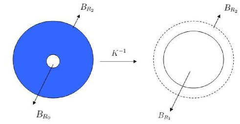
Figure 2: Illustration for magnification: the cloaking device $B_{R_{0}}\bigoplus(B_{R_{0}},\hat{\hat{g}})$ virtually reshapes $B_{R_{0}}$ to $B_{R_{1}}$.

Let $K:\mathbb{R}^{3}\backslash B_{R_{1},p}\mapsto\mathbb{R}^{3}\backslash B_{R_{0},p}$ be defined by

$$x:=K(y)=\begin{cases}\qquad y,&\mbox{for $\|y\|_{p}\geq R_{2}$},\\ \bigg{(}\frac{R_{0}-R_{1}}{R_{2}-R_{1}}R_{2}+\frac{R_{2}-R_{0}}{R_{2}-R_{1}}\|y\|_{p}\bigg{)}\frac{y}{\|y\|_{p}},\ &\mbox{for $R_{0}<\|y\|_{p}<R_{2}$}.\end{cases}$$

It is verified directly that $K$ maps the $l^{p}$-annulus $R_{1}\leq\|y\|_{p}\leq R_{2}$ to the $l^{p}$-annulus $R_{0}\leq\|y\|_{p}\leq R_{2}$. Moreover, $K$ is bijective and both $K$ and $K^{-1}$ are (uniformly) Lipschitz continuous. Set

$$\hat{\hat{g}}=K_{*}g_{0},$$ (2.32)

be the metric in $B_{R_{0},p}^{+}$. Clearly, $\hat{\hat{g}}$ is Euclidean outside $B_{R_{2},p}$.

Proposition 2.8.

The cloaking device $B_{R_{0},p}\bigoplus(B_{R_{2},p}\backslash B_{R_{0},p},\hat{\hat{g}})$ with $\hat{\hat{g}}$ defined in (2.32), reshapes $B_{R_{0},p}$ virtually to $B_{R_{1},p}$. That is, the physical obstacle $B_{R_{0},p}$ with the cloaking material $(B_{R_{2},p}\backslash B_{R_{0},p},\hat{\hat{g}})$ is virtually magnified to the obstacle $B_{R_{1},p}$ with a magnification ratio $\tau:=R_{1}/R_{0}$.

Proof.

Let $u\in H_{loc}^{1}(B_{R_{1},p}^{+})$ be the solution to the Helmholtz equation (2.2)-(2.3) associated with the obstacle $B_{R_{1},p}$. Define $\tilde{u}=K_{*}u\in H_{loc}^{1}(B_{R_{0},p}^{+})$. Again, by the invariance of the Helmholtz equation under transformation together with the fact that $\tilde{u}|_{\partial B_{R_{0},p}}=u|_{\partial B_{R_{1},p}}=0$, we see $\tilde{u}$ is the scattering solution corresponds to $B_{R_{0},p}\bigoplus(B_{R_{0},p}^{+},\hat{\hat{g}})$. That is,

$$A(\theta^{\prime},\theta,k;B_{R_{0},p}\bigoplus(B_{R_{0},p}^{+},\hat{\hat{g}}))=A(\theta^{\prime},\theta,k;B_{R_{1},p}).$$

∎

In Proposition 2.2, we use $F$ to compress the vacuum to achieve a transformation-based minification device, whereas in Proposition 2.8, we use $K$ to loosen up the vacuum to achieve a transformation-based magnification device. Note that $R_{2}>R_{1}$, the cloaking device is of size larger than the virtual obstacle image, though the virtual obstacle could be of size arbitrarily close to the cloaking device. Hence, the cloaking in Proposition 2.8 is not of magnification in the real sense. However, our magnification result is still of particular practical interests, e.g., if one is only interested in recovering an obstacle without knowing a priori that it is cloaked, then the scattering reconstruction will give a virtually magnified obstacle. On the other hand, we would like to mention that in [20, 21, 23], it is demonstrated that a coated cylindrical core can be extended beyond the cloaking shell into the matrix, where the cloaking material must be negative refractive indexed, namely, the corresponding metric $g$ has negative eigenvalues. A general strategy is presented in [14] on how to devise a negative refractive indexed (NRI) cloaking by using the transformation optics. There, the transformation $F$ is neither injective nor orientation-preserving, which maps a right-handed medium to left-handed medium. Based on NRI cloaking, it is shown in [18, 25] that one can virtually reshape a cylindrical perfect conductor of size bigger than the cloaking device. However, all the aforementioned results are essentially based on exerting transformation directly to the analytical solutions, which is not of the main theme of the present paper.

2.4 Virtually reshaping acoustic obstacles by cloaking

Our discussion so far has been mainly concerned with the minification and magnification of obstacles by cloaking. Clearly, we may consider virtually reshaping an obstacle arbitrarily provided a suitable transform can be found with which we can make essential use of the transformation invariance of the Helmholtz equation. Let $M$ be an obstacle with $m$ pairwise disjoint simply connected components $M_{l},l=1,2,\ldots,m$, i.e., $M=\bigcup_{l=1}^{m}M_{l}$. Let $M_{l}\subset M_{l}^{\prime}$ and $M_{l}^{\prime}\cap M_{l^{\prime}}^{\prime}=\emptyset$, for $l,l^{\prime}=1,2,\ldots,m$ and $l\neq l^{\prime}$. Set $M^{\prime}=\bigcup_{l=1}^{m}M_{l}^{\prime}$. Let $\widetilde{M}=\bigcup_{l=1}^{m}\widetilde{M}_{l}$ be another obstacle with $\widetilde{M}_{l}\subset{M}_{l^{\prime}}$. Suppose there exist

$$F_{l}:\mathbb{R}^{3}\backslash\widetilde{M}_{l}\mapsto\mathbb{R}^{3}\backslash M_{l},\quad l=1,2,\ldots,m$$

such that $F_{l}$ is orientation-preserving and invertible with $F_{l}$ and $F^{-1}_{l}$ Lipschitz continuous, and $F_{l}=id$ outside $M_{l}^{\prime}$. Set $g_{l}=(F_{l})_{*}g_{0}$ and let $M_{l}\bigoplus(M_{l}^{\prime}\backslash M_{l},g_{l})$ be a cloaking device for $M_{l}$.

Theorem 2.9.

The cloaking device $M^{\prime}$ virtually reshapes the obstacle $M$ to $\widetilde{M}$. That is,

$$A(\theta^{\prime},\theta,k;M\bigoplus(M^{\prime}\backslash M,g^{\prime}))=A(\theta^{\prime},\theta,k;\widetilde{M}),$$

where $g^{\prime}$ is $g_{l}$ in $M_{l}^{\prime}\backslash M_{l}$.

The proof is already clear from our earlier discussion on minification and magnification. We have several important consequences of the theorem.

Remark 2.10.

Suppose that some of the components of $M$ are uncloaked, say $M_{l}$ for $1\leq l\leq m^{\prime}<m$, and this corresponds to taking $M_{l}=M_{l}^{\prime}=\widetilde{M}_{l}$ and $F_{l}=id$ for $l=1,2,\ldots,m^{\prime}$.

Remark 2.11.

If for some $M_{l}$ being star-shaped w.r.t. certain point, and the transformation $F_{l}^{-1}$ shrinks $M_{l}$ only in the radial direction to $\widetilde{M}_{l}$, then the case with $\widetilde{M}_{l}$ degenerated to a single point corresponds to an ideal cloaking for $M_{l}$. By using a similar argument as that for Proposition 2.6 together with the estimate in Lemma 2.4, one has that $M_{l}$ is invisible to detection. In fact, by repeating the argument, the same conclusion holds when there are more than one obstacle component is perfectly cloaked.

It is noted that in Remark 2.11, the perfectly cloaked obstacle components are required to be star-shaped, and this is because we need to make use of the estimate in Lemma 2.4 to achieve the invisibility. In order to show the prefect cloakings of more generally shaped obstacles, one may need different thoughts.

In the rest of this section, we shall indicate that all our previous results on virtual reshaping in space dimension three can be straightforwardly extended to the two dimensional case. In fact, for two dimensional scattering problem, the (positive definite) acoustic density $\sigma\in L^{\infty}(M^{+})^{2\times 2}$ also transforms according to (2.8). Therefore, the reshaping result presented in Theorem 2.9 is still valid in $\mathbb{R}^{2}$. In order to achieve invisibility for perfect cloaking of star-shaped obstacles in $\mathbb{R}^{2}$, one needs to show a similar estimate to Lemma 2.4. Indeed, replacing $\Phi(x,y)$ by the first kind Hankel function $\frac{i}{4}H_{0}^{(1)}(k|x-y|)$ of order zero in the proof of Lemma 2.4 and using the corresponding mapping properties of the integral operators involved (see [3]), one can obtain by similar arguments the following estimate to the scattering problem in $\mathbb{R}^{2}$ (see (2.18) for comparison),

$$A(\theta^{\prime},\theta,k;M_{1}\cup\mathbb{B})=A(\theta^{\prime},\theta,k;M_{1})+\mathcal{O}(|\log\delta|^{-1})\quad\mbox{as $\delta\rightarrow+0$}.$$ (2.33)

Obviously, with (2.33) one can show that the perfect cloaking of a star-shaped obstacles in $\mathbb{R}^{2}$ makes it invisible to detection.

3 Virtual reshaping for electromagnetic scattering

3.1 The Maxwell’s equations

We define Maxwell’s equations for the scatterer $M\bigoplus(M^{+},g)$ as the one introduced in Section 2.1. Using the metric $g$, we define a (positive definite) electric permittivity tensor $\varepsilon$ and magnetic permeability tensor $\mu$ by

$$\varepsilon^{ij}=\mu^{ij}=|g|^{1/2}g^{ij}\quad\mbox{on\ $M^{+}$}.$$ (3.1)

It is clear that $\varepsilon=(\varepsilon_{ij})_{i,j=1}^{3}$ and $\mu=(\mu_{ij})_{i,j=1}^{3}$ are invariantly defined and transform as a product of a $(+)$-density and a contravariant symmetric two-tensor with the same rule as that for acoustic density $\sigma$ in (2.8). We consider the scattering due to the scatterer $M\bigoplus(M^{+},g)$ corresponding to some incident wave field. The resulting total electric and magnetic fields, $E$ and $H$ in $M^{+}$, are defined as differential 1-forms, given in some local coordinates by

$$E=E_{j}\ dx^{j},\qquad H=H_{j}\ dx^{j}.$$

Here and in the following, we use Einstein’s summation convention, summing over indices appearing both as sub- and super-indices in formulae. Then $(E,H)$ satisfies Maxwell’s equations on $(M^{+},g)$ at frequency $k$

$$dE=ik*_{g}H,\quad dH=-ik*_{g}E,$$ (3.2)

where $*_{g}$ denote the Hodge-operator on $1$-forms given by

$$*_{g}(E_{j}\ dx^{j})=\frac{1}{2}|g|^{1/2}g^{jl}E_{j}s_{lpq}dx^{p}\wedge dx^{q}=\frac{1}{2}\varepsilon^{jl}E_{j}s_{lpq}dx^{p}\wedge dx^{q},$$

with $s_{lpq}$ denoting the Levi-Civita permutation symbol, and $s_{lpq}=1$ (resp. $s_{lpq}=-1$) if $(l,p,q)$ is an even (resp. odd) permutation of $(1,2,3)$ and zero otherwise. By introducing, for $H=H_{j}dx^{j}$, the notation

$$(\mbox{curl}\ H)^{l}=s^{lpq}\frac{\partial}{\partial x^{p}}H_{q},$$

the exterior derivative may then be written as

$$d(H_{q}dx^{q})=\frac{\partial H_{q}}{\partial x^{p}}dx^{p}\wedge dx^{q}=\frac{1}{2}(\mbox{curl}\ H)^{l}s_{lpq}dx^{p}\wedge dx^{q}.$$

Hence, in a fix coordinate, the Maxwell’s equations (3.2) can be written as

$$(\mbox{curl}\ E)^{l}=ik\mu^{jl}H_{j},\quad(\mbox{curl}\ H)^{l}=-ik\varepsilon^{jl}E_{j}.$$ (3.3)

Without loss of generality, we take the incident fields to be the normalized time-harmonic electromagnetic plane waves,

$${E}^{i}(x):=\frac{{i}}{k}\mbox{curl}\ \mbox{curl}\,p\,e^{{i}k{x}\cdot\theta},\quad{H}^{i}(x):=\mbox{curl}\,p\,e^{\mathrm{i}k{x}\cdot\theta},$$

where $p\in\mathbb{R}^{3}$ is a polarization. As usual, the radiation fields are assumed to satisfy the Silver-Müller radiation condition. To complete the description, we further assume that the obstacle $M$ is perfectly conducting, and we have the following two types of boundary conditions on $\partial M$: the perfect electric conductor (PEC) boundary condition

$$\nu\times E|_{\partial M}=0,$$

or the perfect magnetic conductor (PMC) boundary condition

$$\nu\times H|_{\partial M}=0,$$

where $\nu$ is the Euclidean normal vector of $\partial M$.

We shall work with $\varepsilon,\mu\in(L^{\infty}(M^{+}))^{3\times 3}$. It is convenient to introduce the following Sobolev spaces

$$H(\mbox{curl};\Omega) =\{u\in L^{2}(\Omega)^{3};\ \mbox{curl}\,u\in L^{2}(\Omega)\},$$

$$H_{loc}(\mbox{curl};M^{+}) =\{u\in\mathscr{D}^{\prime}(M^{+})^{3};\ u\in H(\mbox{curl};M^{+}\cap B_{\rho})$$

$$\hskip 42.67912pt\mbox{for each finite $\rho$ with $M\subset B_{\rho}$}\}.$$

Then it is known that there exists a unique solution $(E,H)\in H_{loc}(\mbox{curl};M^{+})\oplus H_{loc}(\mbox{curl};M^{+})$ to the electromagnetic scattering problem. Moreover, the solution $E(x,k,p,\theta)$ admits asymptotically as $|x|\rightarrow+\infty$ the development (see [3])

$$E(x,k,p,\theta)=E^{i}(x)+\frac{e^{ik|x|}}{|x|}E_{\infty}(\theta^{\prime},k,p,\theta)+\mathcal{O}(\frac{1}{|x|^{2}}),$$ (3.4)

where $\theta^{\prime}=x/|x|\in\mathbb{S}^{2}$. The analytic function $E_{\infty}(\theta^{\prime},k,p,\theta)$ is known as the electric far-field pattern. Similar to Definition 2.1, we introduce

Definition 3.1.

We say that $M\bigoplus(M^{+},g)$ (virtually) reshapes the obstacle $M$ to another obstacle $\widetilde{M}$, if the electric far-field patterns coincide for $M\bigoplus(M^{+},g)$ and $\widetilde{M}$, i.e.

$$E_{\infty}(\theta^{\prime},k,p,\theta;M\bigoplus(M^{+},g))=E_{\infty}(\theta^{\prime},k,p,\theta;\widetilde{M}).$$

We would also like to remark that the cloaking device in Definition 3.1 can also be written as $M\bigoplus(M^{+},\varepsilon,\mu)$ according to the correspondence (3.1), where $\varepsilon$ and $\mu$ are respectively, electric permittivity and magnetic permeability for the cloaking medium.

3.2 Virtually reshaping electromagnetic obstacles by cloaking

We consider the virtual reshaping for electromagnetic obstacles by cloaking. Let $M=\bigcup_{l=1}^{m}M_{l}$, $M^{\prime}=\bigcup_{l=1}^{m}M_{l}^{\prime}$, $\widetilde{M}=\bigcup_{l=1}^{m}\widetilde{M}_{l}$ and $F_{l},l=1,2,\ldots,m$ be those introduced in Section 2.4. Furthermore, we assume that $F_{l}$ is normal-preserving in the sense that

$$\tilde{\nu}_{l}=\nu_{l}\circ F_{l},\quad l=1,2,\ldots,m,$$

where $\tilde{\nu}_{l}$ and $\nu_{l}$ are, respectively, the Euclidean normals to $\partial\widetilde{M}_{l}$ and $\partial M_{l}$. E.g., if $\widetilde{M}_{l}$ and $M_{l}$ are both star-shaped w.r.t. the origin, say $\partial\widetilde{M}_{l}=\tilde{r}(\theta)\theta$ and $\partial M_{l}=r(\theta)\theta$ with $\tilde{r}/r=c$ being some constant, then $F_{l}$ is normal-preserving since one has

$$\tilde{\nu}_{l}|_{\tilde{r}(\theta)\theta}=\nu_{l}|_{r(\theta)\theta}=\frac{r(\theta)\theta-\mbox{Grad}r}{\sqrt{r^{2}+|\mbox{Grad}r|^{2}}}.$$

Particularly, if $\widetilde{M}_{l}$ is $l^{p}$-ball shaped, the transformation of the following form

$$F(y)=(a+b\|y\|_{p})\frac{y}{\|y\|_{p}},$$

is normal-preserving, which transforms an $l^{p}$-ball of radius $\tilde{r}$ into another $l^{p}$-ball of radius $r=a+b\tilde{r}$.

Concerning the virtual reshaping, we have

Theorem 3.2.

The cloaking device $M^{\prime}$ virtually reshapes the obstacle $M$ to $\widetilde{M}$. That is,

$$E_{\infty}(\theta^{\prime},k,p,\theta;M\bigoplus(M^{\prime}\backslash M,g^{\prime}))=E_{\infty}(\theta^{\prime},k,p,\theta;\widetilde{M}),$$

where $g^{\prime}$ is $g_{l}$ in $M_{l}^{\prime}\backslash M_{l}$.

Proof.

Let $F:\mathbb{R}^{3}\backslash\widetilde{M}\mapsto\mathbb{R}^{3}\backslash M$ be such that $F|_{M_{l}^{\prime}\backslash\widetilde{M}_{l}}=F_{l}|_{M_{l}^{\prime}\backslash\widetilde{M}_{l}},l=1,2,\ldots,m$ and $F=id$ over $\mathbb{R}^{3}\backslash M^{\prime}$. Let $(E,H)\in H_{loc}(\mbox{curl};\widetilde{M}^{+})\oplus H_{loc}(\mbox{curl};$ $\widetilde{M}^{+})$ be the unique scattering solution corresponding to the perfect conducting obstacle $\widetilde{M}$. Define $\hat{E}=F_{*}E$ and $\hat{H}=F_{*}H$. Clearly, $(\hat{E},\hat{H})\in H_{loc}(\mbox{curl};M^{+})\oplus H_{loc}(\mbox{curl};M^{+})$ according to our requirements on the mappings $F_{l}$’s, $l=1,2,\ldots,m$. Moreover, noting $F_{l}$’s, $1\leq l\leq m$, are normal-preserving, we know $\nu\times\hat{E}|_{\partial M}=0$ (resp. $\nu\times\hat{H}|_{\partial M}=0$) if $\widetilde{M}$ is a perfectly electric conducting obstacle (resp. perfectly magnetic conducting obstacle). Hence, $(\hat{E},\hat{H})$ is the unique solution corresponding to the cloaking device $M\bigoplus(M^{\prime}\backslash M,g^{\prime})$. Therefore, we have

$$E_{\infty}(\theta^{\prime},k,p,\theta;M\bigoplus(M^{\prime}\backslash M,g^{\prime}))=E_{\infty}(\theta^{\prime},k,p,\theta;\widetilde{M}).$$

∎

With Theorem 3.2, all the virtual minification and magnification results for acoustic obstacle scattering can be straightforwardly extended to the electromagnetic obstacle scattering. In order to obtain similar invisibility results for a perfectly conducting obstacle when some of its star-shaped components are perfectly cloaked, we need a lemma similar to Lemma 2.4 in the following for electromagnetic scattering.

Lemma 3.3.

Let $M_{1}$, $\mathbb{B}_{0}$ and $\mathbb{B}$ be the same as those in Lemma 2.4, then we have

$$E_{\infty}(\theta^{\prime},k,p,\theta;M_{1}\cup\mathbb{B})=E_{\infty}(\theta^{\prime},k,p,\theta;M_{1})+\mathcal{O}(\delta)\quad\mbox{as $\delta\rightarrow+0$}.$$ (3.5)

Proof.

We first introduce the space $T^{0,\alpha}(\partial M_{1}),0<\alpha\leq 1$, consisting of the uniformly Hölder continuous tangential fields $a$ equipped with the Hölder norm, and $T^{0,\alpha}_{d}(\partial M_{1})=\{a\in T^{0,\alpha}(\partial M_{1});\mbox{Div}\,a\in C^{0,\alpha}(\partial M_{1})\}$. Similarly, one can introduce $T^{0,\alpha}_{d}(\partial M_{1}\cup\partial\mathbb{B})$. We know the solution $(E,H)\in C^{0,\alpha}(\mathbb{R}^{3}\backslash(M_{1}\cup\mathbb{B}))\oplus C^{0,\alpha}(\mathbb{R}^{3}\backslash(M_{1}\cup\mathbb{B}))$ and can be expressed (cf. [3])

$$E(x)=E^{i}(x) +\mbox{curl}\int_{\partial M_{1}}a_{1}(y)\Phi(x,y)ds(y)+i\int_{\partial M_{1}}\nu(y)\times(S_{0}^{2}a)(y)\Phi(x,y)ds(y)$$

$$+\mbox{curl}\int_{\partial\mathbb{B}}a_{2}(y)\Phi(x,y)ds(y)+i\eta\int_{\partial\mathbb{B}}\nu(y)\times(S_{0}^{2}a_{2})(y)\Phi(x,y)ds(y)$$

and $H(x)=\mbox{curl}E(x)/ik$, where $\eta\neq 0$ is a real coupling parameter. Here, $S_{0}$ is the operator as defined in the proof of Lemma 2.4 but with the integration domains changed according to the context and the densities $a_{1}\in T_{d}^{0,\alpha}(\partial M_{1}),a_{2}\in T_{d}^{0,\alpha}(\partial\mathbb{B})$ satisfy

$$(a+\mathcal{M}_{1}a_{1}+i\mathcal{N}_{1}PS_{0}^{2}a_{1}+\mathcal{M}_{2}a_{2}+i\eta\mathcal{N}_{2}PS_{0}^{2}a_{2})(x)=V(x),\ \ x\in\partial M_{1}\cup\partial\mathbb{B}$$ (3.6)

where $a(x):=a_{1}(x)$ for $x\in\partial M_{1}$ and $a(x):=a_{2}(x)$ for $x\in\partial\mathbb{B}$, and $V(x):=-2\nu\times E^{i}(x)$ for PEC obstacle and $V(x):=-2\nu\times H^{i}(x)$ for PMC obstacle. The operators involved in (3.6) are respectively given by

$$(\mathcal{M}_{1}a_{1})(x):= 2\int_{\partial M_{1}}\nu(x)\times\mbox{curl}_{x}\{a_{1}(y)\Phi(x,y)\}\ ds(y),$$

$$(\mathcal{N}_{1}b_{1})(x):= 2\nu(x)\times\mbox{curl}\ \mbox{curl}\int_{\partial M_{1}}\nu(y)\times b_{1}(y)\Phi(x,y)\ ds(y),$$

$$(\mathcal{M}_{2}a_{2})(x):= 2\int_{\partial\mathbb{B}}\nu(x)\times\mbox{curl}_{x}\{a_{2}(y)\Phi(x,y)\}\ ds(y),$$

$$(\mathcal{N}_{2}b_{2})(x):= 2\nu(x)\times\mbox{curl}\ \mbox{curl}\int_{\partial\mathbb{B}}\nu(y)\times b_{2}(y)\Phi(x,y)\ ds(y),$$

$$Pc:= (\nu\times c)\times c.$$

We again refer to [2, 3] for relevant mapping properties of the above operators. Finally, a similar asymptotic analysis to that implemented in the proof of Lemma 2.4, one can complete the proof. ∎

Clearly, with Lemma 3.3, we have similar invisibility result for electromagnetic scattering as those remarked in Remark 2.11 for acoustic scattering.

References

- [1] Chen, H. and Chan, C. T., Transformation media that rotate electromagnetic fields, Appl. Phys. Lett, 90 (2007), 241105.
- [2] Colton, D. and Kress, R., Integral Equation Method in Scattering Theory, Wiley, New York, 1983.
- [3] Colton, D. and Kress, R., Inverse Acoustic and Electromagnetic Scattering Theory, Second Edition, Springer-Verlag, Berlin, 1998.
- [4] Greenleaf, A., Kurylev, Y., Lassas, M. and Uhlmann, G., Electromagnetic wormholes and virtual magnetic monopoles from metamaterial, Phys. Rev. Lett., 99 (2007), 183901.
- [5] Greenleaf, A., Kurylev, Y., Lassas, M. and Uhlmann, G., Electromagnetic wormholes via handlebody constructions, Comm. Math. Phys., 281, 369 (2008).
- [6] Greenleaf, A., Kurylev, Y., Lassas, M. and Uhlmann, G., Full-wave invisibility of active devices at all frequencies, Comm. Math. Phys., 279, 749 (2007).
- [7] Greenleaf, A., Kurylev, Y., Lassas, M. and Uhlmann, G.,Invisibility and inverse prolems, Bulletin A. M. S., 46 (2009), 55–97.
- [8] Greenleaf, A., Kurylev, Y., Lassas, M. and Uhlmann, G., Full-wave invisibility of active devices at all frequencies, Commu. Math. Phys., 275 (2007), 749–789.
- [9] Greenleaf, A., Lassas, M. and Uhlmann, G., Anisotropic conductivities that cannot detected by EIT, Physiolog. Meas. (special issue on Impedance Tomography), 24, 413 (2003).
- [10] Greenleaf, A., Lassas, M. and Uhlmann, G., On nonuniqueness for Calderón’s inverse problem, Math. Res. Lett., 10, 685 (2003).
- [11] Kirsch, A. and Päivärinta, L., On recovering obstacles inside inhomogeneities, Math. Meth. Appl. Sci., 21 (1999), 619–651.
- [12] Kohn, R., Shen, H., Vogelius, M. and Weinstein, M., Cloaking via change of variables in electrical impedance tomography, Inverse Problems, 24 (2008), 015016.
- [13] Leonhardt, U., Optical conformal mapping, Sciences, 312 (2006), 1777–1780.
- [14] Leohardt, U. and Philbin, T. G. , General relativity in electrical engineering, New J. Phys., 8, 247 (2006).
- [15] Liu, H. Y., Recovery of inhomogeneities and buried obstacles, arXive:0804.0938, 2008.
- [16] Liu, H. Y. and Zou, J., On uniqueness in inverse acoustic and electromagnetic obstacle scattering, Journal of Physics: Conference Series, 124 (2008), 012006.
- [17] Luo, Y., Chen, H., Zhang, J., Ran, L. and Kong, J., Design and analytically full-wave validation of the invisibility cloaks, concentrators, and field rotators created with a general class of transformations, Phys Rev B 77 (2008), 125127.
- [18] Luo, X., Yang, T., Gu, Y. and Ma, H., Conceal an entrance by means of superscatterer, arXiv: 0809.1823, 2008.
- [19] McLean, W., Strongly Elliptic Systems and Boundary Integral Equations, Cambridge University Press, Cambridge, 2000.
- [20] Milton, G. W., Nicorovici, N. P., McPhedran, R. C., Cherednichenko, K. and Jacob, Z., Solutions in folded geometries and associated cloaking due to anomalous resonance, arXiv: 0804.3903, 2008.
- [21] Milton, G. W., Nicorovici, N.-A. P., McPhedran, R. C. and Podolskiy, V. A., A proof of superlensing in the quasistatic regime, and limitations of superlenses in this regime due to anomalous localized resonance, Proc. Roy. Soc. Lond., Ser. A, Math. Phys. Sci., 461 (2005), 3999–4034.
- [22] Nachman, A. I, Päivärinta, L. and Teirilä, A., On Imaging Obstacles Inside Inhomogeneous Media, J. Functional Analysis, 252 (2007), 490–516.
- [23] Nicorovici, N.-A. P., McPhedran, R. C. and Milton, G. W., Optical and dielectric properties of partially resonant composites, Phys. Rev. B, 49 (1994), 8479–8482.
- [24] Pendry, J. B., Schurig, D. and Smith, D. R., Controlling Electromagnetic Fields, Sciences, 312 (2006), 1780–1782.
- [25] Yang, T., Chen, H. Y., Luo, X. and Ma, H., Superscatterer: Enhancement of scattering with complementary media, arXiv:0807.5038, 2008