Effects of partitioning and extrapolation on the connectivity of potential magnetic fields

Abstract

Coronal magnetic field may be characterized by how its field lines interconnect regions of opposing photospheric flux – its connectivity. Connectivity can be quantified as the net flux connecting pairs of opposing regions, once such regions are identified. One existing algorithm will partition a typical active region into a number of unipolar regions ranging from a few dozen to a few hundred, depending on algorithmic parameters. This work explores how the properties of the partitions depend on some algorithmic parameters, and how connectivity depends on the coarseness of partitioning for one particular active region magnetogram. We find the number of connections among them scales with the number of regions even as the number of possible connections scales with its square.

There are several methods of generating a coronal field, even a potential field. The field may be computed inside conducting boundaries or over an infinite half-space. For computation of connectivity, the unipolar regions may be replaced by point sources or the exact magnetogram may be used as a lower boundary condition. Our investigation shows that the connectivities from these various fields differ only slightly – no more than 15%. The greatest difference is between fields within conducting walls and those in the half-space. Their connectivities grow more different as finer partitioning creates more source regions. This also gives a quantitative means of establishing how far away conducting boundaries must be placed in order not to significantly affect the extrapolation. For identical outer boundaries, the use of point sources instead of the exact magnetogram makes a smaller difference in connectivity: typically 6% independent of the number of source regions.

1 Introduction

According to prevailing understanding, coronal activity on the Sun involves energy stored in its magnetic field. The coronal field is stressed as the photospheric regions to which it is anchored slowly evolve. In order to build a quantitative model based on this insight it is essential to quantify how the coronal field links these photospheric regions – its connectivity.

Several previous studies have focused on local properties of magnetic connectivity as characterized by the point-wise mapping of positive footpoints to negative footpoints (Seehafer, 1986; Low, 1987; Inverarity & Titov, 1997; Titov et al., 2002, 2003). This mapping is discontinuous at coronal current sheets (tangential discontinuities) where reconnection and energy dissipation are particularly rapid. Regions where the mapping is extremely distorted, called quasi-separatrix layers, may play an equally significant role in these processes as well (Longcope & Strauss, 1994; Priest & Démoulin, 1995; Démoulin et al., 1996, 1997)

While reconnection is a local process, energy storage is global, so its study requires a global characterization of connectivity. For example, when two active regions interact magnetically, there is a change in connectivity whereby new field lines are forged to connect the positive polarity of one to the negative polarity of the other (Sweet, 1958; Longcope et al., 2005). One method of quantifying the global connectivity is to group photospheric footpoints into a number of unipolar regions. This is a tacit step in, for example, the above reference to the “positive polarity of the active region”. Coronal field lines are then categorized by the regions to which their positive and negative footpoints belong.

Global connectivity may be used to quantify the energy stored as coronal field evolves. Barring magnetic reconnection, emergence or submergence, the total flux in each connection is preserved even as the photospheric regions move and deform. The preservation of connection fluxes constitutes a set of constraints which can be used to place a lower bound on the coronal magnetic free energy (Longcope, 2001).

The process of grouping photospheric footpoints into unipolar regions, called partitioning, is natural in certain idealized models (Sweet, 1958; Gorbachev & Somov, 1988; Brown & Priest, 1999) or in the flux elements of the quiet Sun (Schrijver et al., 1997; Hagenaar, 2001; Parnell, 2002; Welsch & Longcope, 2003; Close et al., 2004; DeForest et al., 2007). Magnetograms of real active regions, on the other hand, show photospheric field distributed in a complex pattern whose reduction to regions is less straightforward. One algorithm developed by Barnes et al. (2005) uses the vertical field in a gradient-based tessellation method (Hagenaar et al., 1997). This breaks an active region into anywhere from dozens to hundreds of unipolar photospheric regions, depending on algorithmic parameters. Significantly, the regions identified by the algorithm track inferred photospheric motions (Longcope et al., 2007), so their connectivity can be used to bound coronal energy. Larger numbers of regions will lead to a larger number of constraints, and therefore a more restrictive lower bound on free energy (Longcope, 2001; Longcope & Beveridge, 2007).

The connectivity between photospheric regions depends entirely on the coronal magnetic field anchored to it. Since high spatial resolution measurements are made only at the lowest level of the atmosphere, such as the photosphere, it is necessary to extrapolate these data into the corona before connectivity can be determined. There are numerous methods for performing this extrapolation (see McClymont et al., 1997, for a review) and each one will produce a different connectivity. The most sophisticated class of methods, the non-linear force-free field (NLFFF) models, includes at least a half dozen variants, many of which have recently been inter-compared in a series of investigations (Schrijver et al., 2006; Metcalf et al., 2008; Schrijver et al., 2008). The connectivity was used as a basis of comparison in one of these investigation (Metcalf et al., 2008), and it was found that the different NLFF fields produced by these methods each induced a different connectivity. Indeed, the differences in connectivity tended to be large even when other metrics showed reasonable agreement between an extrapolation and the model field. It is therefore essential to understand how much the connectivity might vary under different extrapolations. This is the objective of the present study.

At the opposite extreme to NLFFF models is the potential field extrapolation, which assumes the corona to be current-free. This assumption leads to a well-posed mathematical problem whose solution is relatively straightforward. Nevertheless, several versions of the potential field are possible depending on the treatment of the boundaries. For example, the magnetogram of a single active region can be extrapolated onto a finite computational grid, into an infinite half space, or into a spherical corona inside a source surface. Each choice has advantages and all are in common use. Since these fields are all different, it is to be expected that each will produce a different connectivity.

In this work we will explore the difference in connectivity produced by different methods of field extrapolation. Since the principles of potential field extrapolation are so simple and well understood, we restrict our investigation to these alone. We will explore the differences produced by different treatments of the boundaries when making potential field extrapolations. In addition to their many other complications, sophisticated extrapolation methods, such as the NLFFF, must choose between these same boundary conditions. It is therefore worth quantifying the effect of these choices on connectivity before considering the effects of more complex extrapolations.

When a coronal field model is to be used only to compute connectivity between unipolar photospheric regions, it is possible to replace those regions by magnetic point charges. The result, known as a magnetic charge topology model (MCT), is a kind of field commonly used to study magnetic topology (Baum & Bratenahl, 1980; Gorbachev & Somov, 1989; Brown & Priest, 1999) as well as to quantify connectivity in observed fields (Longcope & Silva, 1998; Longcope et al., 2005, 2007). Point magnetic charges situated on the photospheric level create certain unphysical artifacts, such as divergent magnetic field. These artifacts are absent from more traditional extrapolations which take the magnetogram itself for the lower boundary condition. MCT models do, however, offer the advantage that their topologies may be rigorously and systematically characterized (Longcope & Klapper, 2002; Beveridge & Longcope, 2005). Furthermore, a potential MCT field in an unbounded half space takes the form of an analytic sum whose evaluation does not require a computational grid.

While it is clear that point charges introduce tremendous errors in local properties of the magnetic field, it is not clear how much they affect its global connectivity. Away from a given unipolar region, the potential field will be dominated by its lowest multipole moments, monopole and dipole. These terms are exactly matched by a single point charge. In this work we quantify the difference in connectivity produced by using point charges in a potential field extrapolation.

In order to make a realistic comparison of connectivities we use a magnetogram of an actual active region. This magnetogram is analyzed using the Barnes et al. (2005) partitioning algorithm with a range of different parameters. The resulting partitions consist of anywhere from 35 to 395 different unipolar regions. We compute connectivities between these regions using four different potential magnetic field extrapolations. We find that the connectivity of a given partition varies by no more than 15% regardless of what potential field extrapolations is used. Among the extrapolations, the choice of outer boundary makes the greatest difference. The use of point sources changes the connectivity by roughly 6% (in this case) regardless of how many unipolar regions are present.

The next section reviews the process of partitioning and shows how its parameters affect the result. Section 3 defines the connectivity flux and describes our method for calculating it. The following section describes the different extrapolation methods we explore. The connectivities are then compared in section 5.

2 Partitioning the magnetogram

We begin with the single magnetogram from the Imaging Vector Magnetograph (Mickey et al., 1996, IVM) shown in LABEL:1. The magnetogram is of AR 8636 from 23 July 1999, and includes most of the flux obviously belonging to the active region (AR). The inversion of the spectra to produce magnetic field maps is described in Leka & Barnes (2003), while the ambiguity inherent in the observed transverse component of the field was resolved using the method described in Canfield et al. (1993). The three vector components of the resulting vector magnetic field are used to compute the vertical (i.e. radial) component in each pixel, $B_{z}(x,y)$. These values form a $237\times 202$ array of $1.1^{\prime\prime}\times 1.1^{\prime\prime}$ pixels within the plane of the sky. Since the active region is relatively close to disk center, and we are using the magnetogram for illustration purposes, we do not project the image onto the solar surface. Instead we perform all analysis within the plane of the sky.

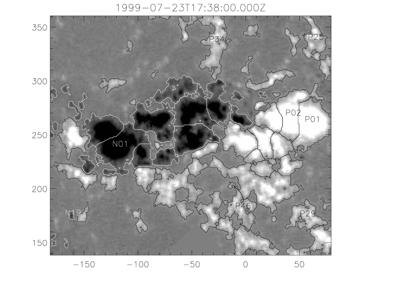
Figure 1: The vertical field, $B_{z}(x,y)$ from the IVM magnetogram of AR 8363 (grayscale). Axes give coordinates in arcseconds from disk center. Curves outline the regions from a partition with saddle level of $B_{\rm sad}=100$ G and smoothing of $h=1.0$ pixel. Several regions are labeled for future reference.

It is evident from the cumulative histograms of positive and negative pixels, shown in LABEL:2, that the data are dominated by positive flux. Positive pixels ($B_{z}>0$) account for $\Phi_{+}=5.1\times 10^{6}$ G arcsec², while negative pixels compose less than two thirds of these values $\Phi_{-}=3.2\times 10^{6}$ G arcsec². (Had the radial field been mapped to the solar surface the fluxes would have been $2.9\times 10^{22}$ Mx and $1.8\times 10^{22}$ Mx respectively.) It can be seen from the histogram that field stronger than 500 G, which accounts for $\simeq 2\times 10^{6}$ G arcsec², is much better balanced; most of the excess positive flux is weaker than this. This apparent imbalance probably arises from the exclusion from the IVM field of view, of an extended, diffuse region of negative polarity to the East. This is possibly part of an older, decaying AR into which 8636 emerged. There is also an excluded region of more positive polarity to the South of the IVM field of view.

Figure 2: A cumulative histogram of the IVM magnetogram from LABEL:1. Solid and dashed lines show the amount of magnetic flux in the plane-of-the-sky (in G$\times$ square-arc-seconds) above a given field strength, in positive and negative polarity respectively. The plus and times mark the amount included within regions; the threshold is $B_{\rm th}=76.9$ G.

Some degree of flux imbalance is inevitable in any magnetogram data. Consequently, any method of magnetic extrapolation and any determination of magnetic connectivity, must somehow accommodate imbalance. Our example, with its extreme degree of imbalance, will bring these issues to the fore. Moreover, we show below that connections outside the AR are quantified more accurately and with less computation in cases of very strong imbalances. It is for these reasons that we select the IVM data from LABEL:1 for the present study.

The magnetogram is next subjected to a process called partitioning (Barnes et al., 2005; Longcope et al., 2007) whereby pixels are grouped into unipolar regions. Pixels with field strength below a cutoff, here set to the $3\sigma$ noise level, $B_{\rm th}=76.9$ G, are discarded, and the remaining pixels are grouped using a gradient-based tessellation scheme (Hagenaar et al., 1997). This grouping uses the gradient of a field constructed by convolving $B_{z}$ with the kernel function

$$K_{h}(x,y)~{}=~{}{h/2\pi\over(x^{2}+y^{2}+h^{2})^{3/2}}~{}~{}.$$ (1)

This function integrates to unity over the entire plane, and to $\sqrt{1/2}$ within a circle of radius $h$. It therefore smoothes out fluctuations in $B_{z}$ on scales smaller than $\sim h$. The function $K_{h}$ was chosen because it is the Green’s function for potential extrapolation upward from an unbounded plane to a height $h$. The convolution $K_{h}*B_{z}$ therefore resembles the vertical field within the plane $z=h$.

The gradient-based tessellation assigns a unique region label to every local maximum in the smoothed field $|K_{h}*B_{z}|$ for which $|B_{z}|>B_{\rm th}$. The label from a given maximum is given to all pixels which are strictly downhill with respect to $|K_{h}*B_{z}|$, and also have $|B_{z}|>B_{\rm th}$. The resulting regions are separated by areas where $|B_{z}|<B_{\rm th}$, or by internal boundaries emanating from saddle points in the convolution $|K_{h}*B_{z}|$. The next step, called saddle-merging, eliminates any internal boundary at whose saddle point $|B_{z}|$ is greater than a value ${\rm min}(|B_{\rm pk}|)-B_{\rm sad}$, where $B_{\rm pk}$ are the values at the neighboring peaks, and $B_{\rm sad}$ is a parameter of the partitioning. The regions are merged by relabeling the smaller one with the region number of the larger. Of the remaining regions, any which have flux less than $10^{3}$ G arcsec² are discarded.

The partition of a particular magnetogram depends critically on the parameters $h$ and $B_{\rm sad}$, as illustrated by LABEL:3. Increasing the smoothing-kernel width $h$ diminishes the number of local maxima. The result is fewer regions which are consequently larger. Similarly, increasing $B_{\rm sad}$, eliminates more internal boundaries, again yielding fewer regions. The progression is evident in LABEL:3 by scanning up the columns or rightward along the rows. The parameters on the upper right ($h=2.0^{\prime\prime}$, $B_{\rm sad}=200$ G) partition the entire magnetogram into in $N=40$ regions, while those in the lower left ($h=0.1^{\prime\prime}$, $B_{\rm sad}=10$ G) partition it into $N=395$.

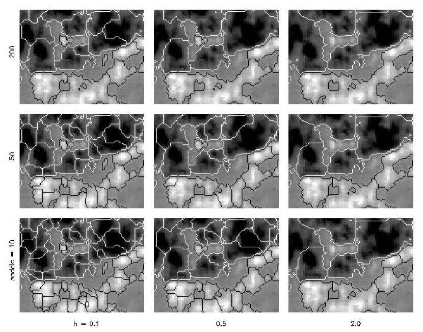
Figure 3: A subsection of the magnetogram (see LABEL:1) partitioned using different parameters. The columns show the smoothing parameters $h=0.1$ pixel (left), $0.5$ (center) and $2.0$ (right). The rows show the saddle-merging levels $B_{\rm sad}=10$ G (bottom), $50$ G (middle) and $200$ G (top). Note that increased smoothing removes the small positive polarity area surrounded by negative polarity, while increased saddle-merging simplifies it to a single partition without removing it.

Region ${\cal R}_{a}$ from a given partitioning is a set of pixels in which $B_{z}$ is of the same sign: the region is unipolar. The region may be characterized by its signed net flux

$$\Phi_{a}~{}=~{}\int\limits_{{\cal R}_{a}}B_{z}(x,y)\,dx\,dy~{}~{},$$ (2)

and its centroid location

$$\bar{{\bf x}}^{a}~{}=~{}\Phi_{a}^{-1}\int\limits_{{\cal R}_{a}}{\bf x}\,B_{z}(x,y)\,dx\,dy~{}~{}.$$ (3)

(We write integrals for mathematical clarity, but these are actually computed as sums over pixels in ${\cal R}_{a}$ multiplied by the pixel area $A_{\rm pix}=1.21$ arcsec².)

Further characterization of a region is provided by its quadrupole moment

$$Q^{a}_{ij}~{}=~{}\Phi_{a}^{-1}\int\limits_{{\cal R}_{a}}(x_{i}-\bar{x}^{a}_{i})(x_{j}-\bar{x}^{a}_{j})\,B_{z}(x,y)\,dx\,dy~{}~{},$$ (4)

where $i$ and $j$ are component indices for the horizontal vectors (either $1$ or $2$). One measure of a region’s horizontal extent is its radius of gyration

$$r_{g}^{a}~{}=~{}\sqrt{Q^{a}_{11}+Q^{a}_{22}}~{}~{}.$$ (5)

Its elongation may be characterized by

$$\varepsilon^{a}~{}=~{}1-{\lambda^{a}_{<}\over\lambda^{a}_{>}}~{}~{},$$ (6)

where $\lambda^{a}_{<}$and $\lambda^{a}_{>}$ are the smaller and larger eigenvalue of $Q^{a}_{ij}$. Since $Q_{ij}$ is positive definite the elongation parameter will lie in the range $0\leq\varepsilon<1$. An axi-symmetric flux distribution will have $\varepsilon=0$, while a very long distribution will have $\varepsilon\simeq 1$.

For a given choice of parameters, $h$ and $B_{\rm sad}$, the partitioning algorithm will break a magnetogram into regions with various characteristics, $\Phi_{a}$ and $r_{g}^{a}$. The partitioning may be characterized as a whole using a flux-weighted average of each characteristic

$${\langle{f}\rangle}~{}=~{}{\sum\limits_{a}|\Phi_{a}|f_{a}\over\sum\limits_{a}|\Phi_{a}|}~{}~{}.$$ (7)

Figure 4 shows the flux-weighted averages of quantities arising from partitions with different parameters. Even as the parameters cover a rectangle of $h$ and $B_{\rm sad}$ most of the averaged values fall on a single curve ordered by the total number of regions $N$. The average elongation, ${\langle{\varepsilon}\rangle}$ (b) decreases slightly from $0.4$ to $0.3$ as $N$ increases from $40$ to $400$. It would seem the finer partitionings (smaller $h$ or smaller $B_{\rm sad})$ produce less elongated regions.

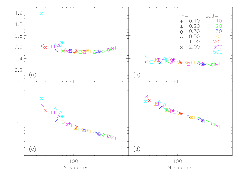
Figure 4: Flux-weighted averages of region characteristics for different partitions. The bottom panels plot the radius of gyration $r_{g}$ (c) and the distance to nearest neighbor, $\Delta_{n}$ (d), both expressed in arcseconds. The top panels show the ratio $r_{g}/\Delta_{n}$ (a) and the region elongation $\varepsilon$ (b). In each plot the value is plotted against the total number of regions in that partition. The different symbols denote different smoothing parameter and colors designate the saddle-merging level. The key for all four plots appear in the upper right of (b). An orange square ($B_{s}=100$ G and $h=1.0$) marks the partition from LABEL:1 with its $N=70$ regions.

The average radius of gyration (c) shows a far more pronounced decrease with increasing number. Clearly finer partitioning produces regions which are generally smaller. The panel to its right, (d), plots the distance, denoted $\Delta_{a}$, from the centroid of region $a$ to the nearest neighboring centroid of either polarity. Its flux-weighted average falls along the curve ${\langle{\Delta_{a}}\rangle}=171N^{-1/2}$. Had the centroids been scattered randomly over the magnetogram their nearest-neighbor distance would tend toward ${\langle{\Delta_{a}}\rangle}=120N^{-1/2}$, at large $N$ (Kendall & Moran, 1963). The median value of $\Delta_{a}$ does, in fact, approximate this curve, but the flux-weighted mean is dominated by larger regions which tend to be further from their neighbors. This tendency leads to the larger coefficient.

3 Connectivity

The connectivity between regions can be found given some coronal field anchored to the partitioned photospheric field. There is a connection between source regions $a$ and $b$ if a coronal field line has one foot in positive region ${\cal R}_{a}$ and the other in negative region ${\cal R}_{b}$. Figure 5 is a schematic depiction of all connections produced by a particular field anchored to the partitioning from LABEL:1.

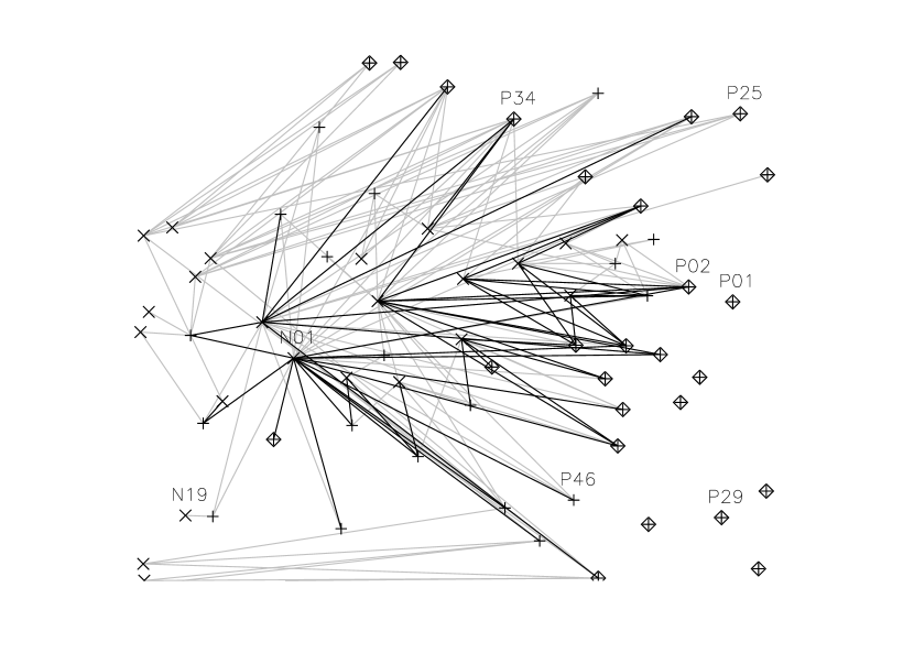
Figure 5: A schematic diagram of the connections between source regions from LABEL:1, induced by coronal field $MB$. Centroids of positive and negative regions are denoted by pluses and times. Connections with flux in excess of $0.25\%$ of $\Phi_{\rm tot}$ are represented by dark lines, those with less by light lines. Diamonds surround regions with connections to infinity.

The connection between region ${\cal R}_{a}$ and ${\cal R}_{b}$ can be quantified by the connection flux, $\psi_{ab}$ (the first index will always designate the positive source region). If a connection exists between these regions then $\psi_{ab}>0$; if they are unconnected then $\psi_{ab}=0$. All of the flux anchored to negative region ${\cal R}_{b}$ must have originated in some positive region, so

$$|\Phi_{b}|~{}=~{}\sum_{a\in{\cal S}_{+}}\psi_{ab}~{}~{},$$ (8)

where ${\cal S}_{+}$ is the set of all positive regions. A similar expression holds for positive region $a$

$$\Phi_{a}~{}=~{}\sum_{b\in{\cal S}_{-}}\psi_{ab}~{}~{},$$ (9)

except that ${\cal S}_{-}$ includes an extra source to account for field lines extending to “infinity” due to the net positive imbalance. This new source has flux $|\Phi_{\infty}|=\Phi_{+}-|\Phi_{-}|$, in order to account for all flux which cannot close in a photospheric negative source. With the inclusion of infinity as a negative source, sources of each sign will have the same net flux

$$\Phi_{\rm tot}~{}=~{}\sum_{a\in{\cal S}_{+}}\Phi_{a}~{}=~{}-\sum_{b\in{\cal S}_{-}}\Phi_{b}~{}=~{}\sum_{a\in{\cal S}_{+}}\sum_{b\in{\cal S}_{-}}\psi_{ab}~{}~{}.$$ (10)

This is the total amount of flux in the field.

The connection flux $\psi_{ab}$ can be estimated using a Monte Carlo method (Barnes et al., 2005). A number $n_{a}$ of footpoints are selected randomly within positive source region ${\cal R}_{a}$. Each field line is then followed to its other end (or to a distance from which which it will not return). The number which end at region ${\cal R}_{b}$ is designated $m_{ab}$. Field lines are then randomly initialized from negative regions (except infinity) and traced backward to their positive source region. The number initiated in ${\cal R}_{b}$ which “terminate” in ${\cal R}_{a}$ are denoted $m_{ba}$. The Bayesian estimate of the connection flux $\psi_{ab}$ (Barnes et al., 2005) combines the information from tracing in both directions as

$$\psi_{ab}~{}=~{}{m_{ab}+m_{ba}\over{n_{a}/\Phi_{a}+n_{b}/|\Phi_{b}|}}~{}~{}.$$ (11)

Since no points were initiated at infinity, $n_{b}=0$ and $m_{ba}=0$ for that case ($b=\infty$). The estimate then reduces to $\psi_{ab}=(m_{ab}/n_{a})\Phi_{a}$.

Expression (11) is a Monte Carlo estimate of the actual connection flux so it will include some statistical error. This error can be estimated using the (approximately) Poisson statistics of the counts $m_{ab}$ and $m_{ba}$. If an actual connection includes very little flux it is possible that none of the randomly generated field lines will sample it and $m_{ab}=m_{ba}=0$. The probability that an actual connection will be erroneously missed for this reason is

$$P_{\rm miss}(\psi_{ab})~{}=~{}e^{-\psi_{ab}/\tilde{\phi}_{0}}~{}~{},$$ (12)

where $\tilde{\phi}_{0}=1/(n_{a}/\Phi_{a}+n_{b}/|\Phi_{b}|)$. Naturally the use of more points (i.e. larger values of $n_{a}$ and $n_{b}$) will make this increasingly unlikely. Nevertheless, there will always be a possibility that some number of very small connections have remained undetected. For one particular case (later defined as field $PH$) a topological analysis of the connections revealed that 10 of 109 connections were erroneously missed by the Monte Carlo method.

4 Coronal fields

4.1 Different potential fields

In order to define connectivity it is necessary to compute the entire coronal field anchored to the photospheric field $B_{z}$. Although we have chosen to restrict consideration to potential fields, $\nabla\times{\bf B}=0$, there are several different ways to compute a potential field from magnetogram data. We consider a variety of these fields and study the effect on the connectivity of the differing fields.

One option is to compute the potential field within a rectangular $L_{x}\times L_{y}\times L_{z}$, box, ${\cal B}$, with a lower boundary at the magnetogram, $z=0$. The four lateral boundaries are perfect conductors (${\bf\hat{n}}\cdot{\bf B}=0$) positioned along the edges of the magnetogram. The vertical field at the lower boundary, $B_{z}(x,y,0)$, is taken from the magnetogram and is therefore not balanced. An equal net flux must cross the upper boundary or no solution would be possible for which $\nabla\cdot{\bf B}=0$. We achieve this with a uniform vertical field along the upper boundary: $B_{z}(x,y,L_{z})=|\Phi_{\infty}|/(L_{x}L_{y})$. A field line crossing this upper boundary is designated as a connection to infinity. We choose to place this upper boundary at $L_{z}=220^{\prime\prime}$, approximately equal to $L_{y}$, and slightly less than $L_{x}$.

The alternative to the computational box ${\cal B}$ is to use a coronal field extending throughout the entire half-space $z>0$. Such an unbounded field is computed, in principle, by convolving the field at $z=0$ with a Green’s function for a point magnetic charge at $z=0$. In practice we compute either a portion of the field on a grid or compute it along a field line as we trace it. We distinguish between the box boundary and the half-space using superscripts $B$ and $H$ respectively.

For the purposes of computing connections between unipolar regions it is possible to replace each region with a point source. Region ${\cal R}_{a}$ is replaced with a magnetic charge of strength $q_{a}=\Phi_{a}/2\pi$ at position $\bar{{\bf x}}^{a}$ on the photospheric plane, $z=0$. This matches a multipole approximation of the potential field from ${\cal R}_{a}$ up to the dipole term, thus it is expected to be accurate at distances $|{\bf x}-\bar{{\bf x}}^{a}|\gg r_{g}^{a}$. Fields computed using point sources will be assigned a superscript $P$. With this simplification the convolution required for the half-space computation becomes

$${\bf B}^{\rm(PH)}({\bf x})~{}=~{}\sum_{a}{\Phi_{a}\over 2\pi}\,{{\bf x}-\bar{{\bf x}}^{a}\over|{\bf x}-\bar{{\bf x}}^{a}|^{3}}~{}~{},$$ (13)

where the sum is over all $N$ sources, not including infinity.

An alternative to photospheric point sources is to compute a potential field matching the magnetogram pixel-for-pixel. Field vectors are computed on a three-dimensional uniform cartesian grid, for example within ${\cal B}$. In order that each field line have a defined connectivity magnetogram pixels which do not belong to a source region are set to zero. The resulting magnetograms differ slightly for different partitionings, but for most cases $\Phi_{+}=4.7\times 10^{6}$ G arcsec² and $\Phi_{-}=2.7\times 10^{6}$ G arcsec². Fields anchored in this way are designated by a superscript $M$.

The field ${\bf B}^{(MB)}$, bounded by conducting boundaries, is readily computed on the Cartesian grid using Fourier methods. The extrapolation into the half-space, ${\bf B}^{(MH)}$, is done onto a larger Cartesian grid which we call ${\cal G}_{MH}$. The field at any grid point can be found by convolving the entire magnetogram with the half-space Green’s function. Performing the convolution for every grid-point is very time-consuming so we use it only for points along the boundary $\partial{\cal G}_{MH}$. We then use the efficient Fourier techniques to compute the interior potential field matching these boundary values. It is noteworthy that flux crosses the boundaries $\partial{\cal G}_{MH}$, so these are not genuine boundaries of the field.

4.2 Calculating the connection fluxes

For each type of coronal field, connection fluxes $\psi_{ab}$ are computed using the Monte Carlo estimate in eq. (11). Approximately $n_{a}=|\Phi_{a}|/(2\phi_{0})$ field lines are initiated on source $a$, where we have chosen $\phi_{0}=10\,$ G arcsec². The smallest flux reported will be $\psi_{ab}\simeq\phi_{0}$, for example when $m_{ab}=1$ and $m_{ba}=0$. With our choice of $\phi_{0}$, every source will have at least 50 lines, and the largest will have $n_{P01}\simeq 4\times 10^{4}$. One complete estimate, such as the one shown in LABEL:5 requires $(\Phi_{+}+|\Phi_{-}|)/20\simeq 3.7\times 10^{5}$ field lines be traced.

Field line initialization is different for the cases anchored to point sources than for those anchored to magnetograms. In the point-source cases, the $n_{a}$ points for a given source are randomly generated with a uniform distribution over a very small hemisphere centered at the point source. The radius of the hemisphere is set to be small enough that the magnetic field is directed roughly radially outward (inward) from the positive (negative) source.

For magnetogram cases the extended region ${\cal R}_{a}$ is a set of $P_{a}$ pixels. First, a list of $n_{a}$ pixels are randomly generated so as to sample each pixel in ${\cal R}_{a}$ with probability proportional to its field strength ($p=A_{\rm pix}B_{z}/\Phi_{a}$). Since $n_{a}\gg P_{a}$, typically, the list will include many duplicate pixels. For each random pixel (including all duplications) an initial point is randomly generated with a uniform distribution over the pixel. Thus no two field lines from the same pixel will begin at the same point. The subsequent field line integration uses tri-linear interpolation to calculate ${\bf B}({\bf x})$, so different points within the same pixel will belong to different field lines.

Using these methods we estimate the connectivity of a given field according to Equation (11). As an illustration, consider the field ${\bf B}^{(MB)}$ from the partition shown in LABEL:1. Our estimate, shown in LABEL:5, includes 198 different connections between its $N=70$ sources (71 including $\infty$). These connections are quantified by their connection fluxes, $\psi_{ab}$, plotted in LABEL:6. The connections to a given source fall along a vertical line below the diagonal, $\psi_{ab}=\Phi_{a}$ (dotted) in the lower panel. The number of connections to that source, called its degree $d_{a}$, is plotted above its flux in the upper panel.

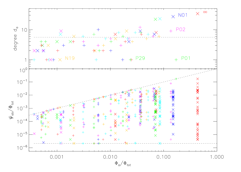
Figure 6: The connection fluxes $\psi_{ab}$ from the field depicted in LABEL:5. The bottom panel plots the flux $\psi_{ab}$ against the flux of its sources, $\Phi_{a}$ (as a $+$) and $|\Phi_{b}|$ (as a $\times$). The sloped and horizontal dotted lines show the maximum and minimum possible values: $\psi_{ab}=\Phi_{a}$ and $\phi_{0}$ respectively. Colors are used to differentiate the different sources, whose connections fall along a vertical line. On each axis the fluxes are normalized to the total, $\Phi_{\rm tot}$. The top panel plots the number of connections to each source, $d_{a}$. Several of the sources are labeled for reference. The horizontal dotted line shows the mean degree, $\bar{d}_{a}=5.65$.

Some sources, such as $P01$ or $N19$, have only a single connection ($d_{a}=1$) and are called leaves. In LABEL:5, leaves appear at the end of a single line ($N19$) or as an isolated diamond ($P01$). In the lower panel of LABEL:6, the fluxes of a leaf connection naturally fall on the dotted diagonal since all the flux from that source belongs to that single connection.

In contrast to the leaf connections there are several sources, such as $N01$ with many connections ($d_{N01}=27$). Given $C=198$ connections to $N+1=71$ sources, the average source must connect to $\bar{d}_{a}=2C/(N+1)=5.65$ sources: the value marked by the dotted line in the upper panel. (The factor of two arises from the fact that each connection is incident on two different sources: one positive and one negative). There is a notable tendency for larger sources, especially larger negative sources, to have more connections. As a consequence of this tendency, the flux-weighted average, Equation (7), of the degree is ${\langle{d_{a}}\rangle}=9.35$ in this case.

4.3 Connections to infinity

In each different magnetic field there is open flux, represented by field lines connected to infinity (formally a negative source). In the $MB$ and $PB$ fields, an open field line is one that terminates at the upper surface of the box, $z=L_{z}$. The 34 positive sources enclosed by diamonds in LABEL:5 are connected to infinity in the $MB$ field for that partition. These form the connections whose fluxes fall in the right-most vertical row of $\times$s in LABEL:6.

The $PH$ field occupies the entire half space and open flux truly extends outward indefinitely. Far from the AR the field resembles that from a single point charge $|\Phi_{\infty}|/2\pi$; field lines go outward approximately radially. There is a single separatrix surface dividing closed from open flux, and once a field line has been integrated far enough to establish that it lies outside this surface, it may be designated as a connection to infinity.

The separatrix between open and closed field is a dome anchored to a null point located $\sim 327$ arcsec from the center of the AR (the triangle in LABEL:7). The footprint of the dome passes along a series of spines (solid curves) linking positive sources. These sources connect to infinity as well as at least one other negative source, $N02$, inside the dome. Positive sources outside the dome link only to infinity.

Figure 7: The footprint of the separatrix dividing closed from open flux (dashed and solid curves) in the field ${\bf B}^{(PH)}$ from the partition of LABEL:1. Positive and negative sources are denoted by $+$s and $\times$s respectively. Triangles are magnetic null points. The triangle at the far left, lying along the dashed curve, is the negative null whose fan surface is the separatrix. The center of unsigned flux is denoted by a diamond, and the dipole moment about this point is indicated by an arrow. The broken rectangle shows the extent of the magnetogram, and the larger dotted one is the bottom surface of ${\cal G}_{MH}$.

The dipole moment, computed about the center of unsigned flux (diamond in LABEL:7), is $\mu=5.1\times 10^{7}$ G arcsec³, directed $7^{\circ}$ below ${\bf\hat{x}}$ as shown in the figure. A far field with this dipole and the net charge, $q_{\infty}=+|\Phi_{\infty}|/2\pi$ will vanish at one point located a distance

$$r_{0}~{}=~{}2{\mu\over q_{\infty}}~{}\simeq~{}318\,{\rm arcsec}~{}~{},$$ (14)

from the center of unsigned charge. For a region with positive net flux, as we have, the null is situated in the direction opposite to the dipole moment. Clearly this is the approximate location of the null point whose separatrix divides open from closed flux in the $PH$ field. Had the region been more balanced, $q_{\infty}$ would have been smaller and the separation of open from closed flux would have occurred much farther out.

There are 22 positive sources linked to infinity by dint of lying on or outside the separatrix in field $PH$. In contrast, the $MB$, field has 34 sources connected to $\infty$, even though there is the same amount of open flux, $|\Phi_{\infty}|$, in each case. Comparing the labeled sources in Figures 5 and 7, shows that different sources are so connected in the $MB$ and the $PH$ fields. These connections are just some of the differences between the two fields, explored further in the next section.

Establishing and quantifying connections to infinity is particularly challenging for the $MH$ field. Although this field formally extends throughout the half-space, it is known only on a Cartesian grid covering ${\cal G}_{MH}$. A field line can therefore be followed to the boundary of ${\cal G}_{MH}$ but no farther. It is, in principle, possible for field at $\partial{\cal G}_{MH}$ to be directed both inward and outward. When this is the case there must be some field lines which leave the volume where $B_{n}>0$ and return where $B_{n}<0$. Naturally these field lines cannot be followed, so their flux cannot be correctly assigned to a connection. Due to the large flux imbalance in our magnetogram we were able to select a volume ${\cal G}_{MH}$ for which $B_{n}\geq 0$ on all outer surfaces (see LABEL:7). Thus any field line encountering the boundary is necessarily connected to infinity.

In order to assure $B_{n}>0$ on the outer boundary it is necessary (but not sufficient) that ${\cal G}_{MH}$ enclose the separatrix dome in the field ${\bf B}^{(MH)}$. This surface will closely resemble (but not exactly match) the separatrix dome from ${\bf B}^{(PH)}$ since both fields approach the same far-field form. It is evident from LABEL:7 that the base of ${\cal G}_{MH}$ does enclose the latter separatrix. This requirement means ${\cal G}_{MH}$ must be considerably larger than ${\cal B}$, so computations in ${\bf B}^{(MH)}$ are much more expensive than for ${\bf B}^{(MB)}$ or ${\bf B}^{(PB)}$. If the active region had had better flux balance then ${\cal G}_{MH}$ would need to be still larger and computation would have become prohibitively expensive.

5 Comparisons

5.1 Different fields from a single partition

Four different coronal fields can be generated from a single partition in the fashion described above. Each field will contain the same total flux, $\Phi_{\rm tot}$, interconnecting the same $N+1$ sources. The connections will not, however, be the same for the different fields. Figure 8 shows the connection fluxes $\psi^{(MB)}_{ab}$ (the ones from LABEL:6) plotted against those induced by ${\bf B}^{(PB)}$. There are $C^{(MB)}=198$ connections in the former and only $C^{(PB)}=184$ in the latter. Moreover, there are 48 connections in $MB$ which do not appear in $PB$; these appear as diamonds along a vertical line in the central panel. Similarly 34 connections in $PB$ not present in $MB$ form the horizontal row of diamonds. We refer to either of these as singlet connections. The remaining 150 connections, common to both fields, are plotted as $+$s in the central panel.

Figure 8: The fluxes of identical connections from two different fields, $MB$ (vertical axis) and $PB$ (horizontal axis) plotted against one another. Fluxes are normalized to the total $\Phi_{\rm tot}$. Vertical and horizontal dotted lines show the minimum flux, $\phi_{0}$. Singlet connections (absent from one of the fields) appear as diamonds below or to the left of these limits. For example, the vertical line of diamonds are absent from $PB$ but present in $MB$ with fluxes indicated by their position. The diagonal dotted lines mark $\psi_{ab}^{(MB)}=2\psi_{ab}^{(PB)}$ (upper) and $\psi_{ab}^{(MB)}=\psi_{ab}^{(PB)}/2$ (lower). Statistical errors are indicated on a few representative points. Plotted along the right and top are histograms of $\ln\psi_{ab}$ for that field. The number appearing in the histogram gives the total number of connections.

The tendency for common connections ($+$s) to cluster about the diagonal, especially at the upper right, shows that connections have similar fluxes in both fields. The connections falling outside the dotted diagonals (i.e. disagreeing by more than a factor of two) are overwhelmingly dominated by smaller connections: $\psi_{ab}<10^{-3}\Phi_{\rm tot}$. These small connections also compose almost all of the singlet connections in either field. Indeed, a great many of the singlets are so small ($\psi_{ab}\simeq\phi_{0}$) that they had a significant probability of going undetected even in the field where they were found. These tiny connections account for most of the spikes at the small-flux end of each histogram.

The statistical errors from the Monte Carlo calculations are relatively large for small fluxes (found by only a few field lines). On the logarithmic plot, like LABEL:8, the error bars are largest at the bottom or left. Above a value of $\psi_{ab}\simeq 10^{-3}\Phi_{\rm tot}$ statistical errors are less that $0.1\%$ and errors bars are smaller than the symbols.

The impression given by a comparison such as LABEL:8 is that in spite of their differences the two coronal fields induce connections which are largely in agreement. The differences appear mostly in the very small connections. While these are small, most of them lie well above the detection limit, $\phi_{0}$, and thus represent genuine differences. The fact that the differences are in small connections suggests that they will not be of great importance to a model of the field.

In order to weight the most significant flux differences we focus on the difference

$$\Delta\psi_{ab}=\psi_{ab}^{\rm(MB)}-\psi_{ab}^{\rm(PB)}~{}~{}.$$ (15)

Connections with positive difference ($\Delta\psi_{ab}>0$) are those for which $MB$ has excess flux relative to $PB$; these appear above the diagonal in LABEL:8. Using Equation (10) we can show that

$$\sum_{a\in{\cal S}_{+}}\sum_{b\in{\cal S}_{-}}\Delta\psi_{ab}~{}=~{}0~{}~{},$$ (16)

so there will be as much flux in connections with excess ($\Delta\psi_{ab}>0$) as in connections with deficit ($\Delta\psi_{ab}<0$). Figure 9 shows cumulative histograms of the flux differences of each sign. In each case the total discrepancy is $6.80\%$ of $\Phi_{\rm tot}$. The connections are sorted by decreasing magnitude, so the histograms rise sharply at first. Ten to twelve connections account for half the total discrepancy of each sign (shown by diamonds). The rest of the discrepancy occurs in the hundred or so other connections.

Figure 9: Cumulative histograms of the flux differences $\Delta\psi_{ab}$. Those with $\Delta\psi_{ab}>0$ are graphed on the right and the ones with $\Delta\psi_{ab}<0$ are on the left. The differences are sorted by decreasing magnitude, so the upper curves plot the total difference for the $n$ largest differences of that sign. The right axis gives this flux in units of G arcsec² while the left axis gives it in units of $\Phi_{\rm tot}$. The lower curves are for only the singlet connections. A $+$ and $\times$ appears at the extreme values of the total and singlet curves respectively. These extreme values are also projected to the ordinate and abscissa with the same symbol. The sole exception is that the $\times$ on the left gives the sum of the total singlet fluxes of both signs, while the curves show the sums for each sign separately. A $\diamond$ shows half the total discrepancy for each sign of $\Delta\psi_{ab}$.

For a singlet connection, one of the terms on the right of Equation (15) will vanish. The magnitude of the difference will therefore equal the other term. The lower curves in LABEL:9 show histograms formed from the singlet connections alone. The right curve accumulates the differences in the 48 singlet connections in $MB$, while the left accumulates the 34 singlets in $PB$ (for which $\Delta\psi_{ab}<0$). Combining their totals yields $1.05\%\Phi_{\rm tot}$, so singlets contribute only a small fraction to the overall flux discrepancy ($6.80\%$).

The inclusion of two other kinds of coronal field leads to six different pairwise comparisons of the kind just used. Figure 10 shows cumulative histograms like those in LABEL:9, for all six possible flux differences. All histograms have the same $\Upsilon$ shape as the ones in LABEL:9; a few connections account for the majority of the discrepancy. Variation among the three fields seems to be mostly a matter of degree.

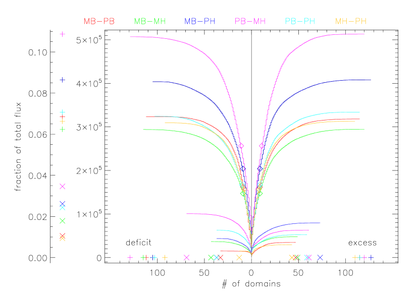
Figure 10: A superposition of cumulative histograms comparing all four different kinds of fields. Each comparison is the same as LABEL:9, but shown in a different color. The color code appears along the top.

The largest discrepancies are between fields differing both in the their anchoring (magnetograms versus points) and their boundaries (box versus half-space): for example between $PB$ and $MH$. The fields differing in only one respect, either anchoring or boundary, have histograms in a cluster below the other two. This tendency is true for both the total histograms (upper curves) and singlet histograms (lower curves).

Making the same plots for many other partitions we find no exceptions to this $\Upsilon$ shape. The histograms therefore differ mostly in their magnitude, which may be summarized by the maximum (marked by a $+$ along the left axes in Figures 9 and 10). We denote this value

$$\Delta\Psi_{X-Y}~{}=~{}\hbox{${1\over 2}$}\sum_{a\in{\cal S}_{+}}\sum_{b\in{\cal S}_{-}}|\psi_{ab}^{(X)}-\psi_{ab}^{(Y)}|~{}=~{}\hbox{${1\over 2}$}\sum_{a\in{\cal S}_{+}}\sum_{b\in{\cal S}_{-}}|\Delta\psi_{ab}|~{}~{},$$ (17)

for a comparison between ${\bf B}^{(X)}$ and ${\bf B}^{(Y)}$ for the same partition. (Here $X$ and $Y$ stand for any of $MB$, $PB$, $MH$ or $PH$.) Thus LABEL:10 is summarized by the values $\Delta\Psi_{PB-MH}=10.8\%$, $\Delta\Psi_{MB-PB}=8.6\%$, $\Delta\Psi_{MB-PB}=6.8\%$, and so forth (in units of $\Phi_{\rm tot}$).

All the connection fluxes are calculated by Monte Carlo methods, so the values of $\psi_{ab}^{(X)}$ and $\psi_{ab}^{(Y)}$ include statistical errors. The sum in (17) will therefore be biased upward, and even an estimate of $\Delta\Psi_{X-X}$ will be positive provided it uses two different estimates of the connectivities from ${\bf B}^{(X)}$. (To see this note that the sum in Equation [17] is over numbers which are never negative and are usually positive due to errors.) We can subtract the expected bias, assuming errors in $\Delta\psi_{ab}$ to have Gaussian distributions, following a procedure described in an appendix. Doing so for $\Delta\Psi_{MB-MB}$, for example, yields a number consistent with zero. Doing so for the red curve in LABEL:10 yields $\Delta\Psi_{MB-PB}=6.6\%\pm 0.25\%$ (the value on the curve, $\Delta\Psi_{MB-PB}=6.8\%$, is therefore biased upward by $\simeq 0.2\%$). Thus there is a true difference between field $MB$ and $PB$, beyond that caused by statistical errors.

The quantity $\Delta\Psi_{X-Y}$ can be considered the connectivity distance between the coronal field models ${\bf B}^{(X)}$ and ${\bf B}^{(Y)}$. When $\Delta\Psi_{X-Y}=0$ the fields are identical, at least with respect to their connectivities. For a given partition there are four different fields separated by six distances. The fields can be represented as vertices of a tetrahedron in a three-dimensional space. The left column of LABEL:11 shows two views of the tetrahedron formed from the histograms in LABEL:10. The distances used in these plots have biases removed.

Figure 11: Tetrahedra formed from the connectivity distances between four fields anchored to different partitions. Each tetrahedron is oriented so that $MB$, $PB$ and $MH$ lie in a plane. The view perpendicular to that plane is shown below and tangent to the plane is shown above, with the same scale. The tetrahedron on the left is from the partition of LABEL:1, whose distances appear in LABEL:10. Distances are in percentages of $\Phi_{\rm tot}$ and horizontal and vertical reference bars are shown ($5\%$ and $10\%$ respectively). The center and right columns are tetrahedra for partitions with $N=108$ and $N=395$ regions. The vertices, labeled on the left, are in the same orientation for all three cases.

If all six distances were exactly the same, they would form a regular tetrahedron. In fact two of the distances, $\Delta\Psi_{PB-MH}$ and $\Delta\Psi_{MB-PH}$, are largest, leading to the extremely flat tetrahedron shown in LABEL:11. The flattened shape is approximately a quadrilateral lying in a plane, with the two large distances forming its diagonals. The sides of the quadrilateral separate vertices (fields) differing in only one respect. The face-on views of the quadrilateral (bottom) are oriented so that horizontal edges separate fields of different anchoring (M vs. P) while vertical edges separate fields of different boundaries (B vs. H).

Performing the same analysis for different partitions gives distances with similar properties, as exemplified by the center and right tetrahedra in LABEL:11. Fields differing in both anchoring and boundaries are furthest apart, so the tetrahedron is flattened into a quadrilateral. Furthermore both instances of a particular difference, such as the anchoring (the horizontal sides in the lower view), result in a similar distance. This makes the quadrilateral into an approximate parallelepiped. For the cases with more sources (center and right) changing boundaries makes the largest differences, so the parallelepipeds tend to be taller than they are wide. Finally, the similarity of the diagonals pushes the shape toward a rectangle.

5.2 Variation in partitions

To see how the above comparisons are affected by different partitioning parameters we perform Monte Carlo calculations for fields from different partitions. The smoothing parameter $h$ is varied from $0.1$ to $2.0$ arcsecs, and $B_{\rm sad}$ from $10$ G to $500$ G.

Once again we find that the different partitioning can be approximately ordered by the number of regions, $N$. Figure 12 shows the average degree of a source region in each of the fields over a range of partitioning. The lower points show the un-weighted average, $\bar{d}_{a}=2C/(N+1)$, as illustrated in LABEL:6. This quantity is very similar, $\bar{d}_{a}\simeq 6$, for all fields and all levels of partitioning. It seems that the number of connections scales as $C\sim 3N$ even as the number of possible connections goes as $\sim N^{2}$. In contrast, the flux weighted average, ${\langle{d_{a}}\rangle}$, does appear to increase with the number of regions, although perhaps at a power less than $\sim N$. This shows that the largest sources connect to more sources as they become available.

Figure 12: The average degree (number of connections) per source for various fields. Different partitions are plotted versus the number of sources, $N$ as symbols. The average of all fields is plotted as a solid curve. The bottom set are the average, $\bar{d}_{a}=2C/(N+1)$, while the upper are the flux weighted average, ${\langle{d_{a}}\rangle}$ from Equation (7).

Comparisons from the previous section, between all four kinds of field, suggested that it is sufficient to compare only three. The six possible comparisons between all four fields were visualized as a tetrahedron of distances. It was found, however, that these tended to form a flat rectangle, well characterized by two of its sides. Taking advantage of this we consider the fields $MB$, $PB$ and $PH$ for a large number of different partitions. Among the three comparisons there is one differing only by anchoring ($MB$ versus $PB$), one differing only by boundaries ($PB$ versus $PH$) and one differing in both respects ($MB$ versus $PH$).

Finer partitioning (i.e. smaller values of $h$ or $B_{\rm sad}$) result in more source regions, $N$. According to the lower curve in LABEL:12 these sources are interconnected in a proportionately large number of ways, $C$, regardless of which coronal field is used. One expects that subdividing the same total flux, $\Phi_{\rm tot}$, into a larger number of pieces would yield bigger discrepancies, $\Delta\Psi_{X-Y}$. Figure 13 shows that this expectation is borne out when comparing fields with different boundaries, ($PB$ to $PH$, $+$s or $MB$ to $PH$, $\ast$s). These curves trend upward as $N$ increases.

Figure 13: The total connectivity difference, $\Delta\Psi_{X-Y}$, defined in Equation (17) for different fields and different partitions. Comparisons are between fields with different anchoring ($MB-PB$) $\times$, different boundaries ($PH-PB$) $+$, and differing in both ($MB-PH$) $\ast$. All differences are plotted as a percentage of $\Phi_{\rm tot}$. The dashed line shows $(\Delta\Psi^{2}_{MB-PB}+\Delta\Psi^{2}_{PH-PB})^{1/2}$ for comparison.

In keeping with the results of the previous sub-section, the cases which differ in both respects ($\ast$) are separated by the greatest distance. The quantity $(\Delta\Psi^{2}_{MB-PB}+\Delta\Psi^{2}_{PH-PB})^{1/2}$, plotted as a dashed line, appears to match the the asterisks well. This fit corroborates the observation from the previous section that the connectivity distances formed a flat rectangle; the dashed curve is the hypotenuse of a right triangle formed from the other two distances.

A truly remarkable feature of LABEL:13 is that the two bounded fields, differing only in their photospheric anchoring, $MB$ and $PB$, differ by a relatively small amount ($\sim 6\%$) which does not change with finer partitioning. This corroborates the tendency observed in LABEL:11 for the rectangles to grow taller with increasing $N$, without growing wider. So while there are ever more connections being compared, and more positive terms in Equation (17), the total difference does not seem to change. It seems that the difference between using point sources or using the actual magnetogram, is about 6% of the connectivity.

5.3 Variations in box size

We can further explore the effect of outer boundaries by increasing the size of the conducting box. To do this the box ${\cal B}$ is augmented by layers of equal width, $w$, along all boundaries except the bottom ($z=0$). This new domain, called ${\cal B}^{+}$, has conducting boundaries on the four lateral walls and a uniform field at the top boundary $z=L_{z}+w$. For the field, $PB^{+}$, the lower boundary has the same $N$ point sources located at the same positions within the central $L_{x}\times L_{y}$ square. The field is computed on a grid with cubic pixels, $1.1^{\prime\prime}$ on side, just as in the $PB$ field.

Connectivities are computed in fields $PB^{+}$ anchored to point sources from the partition with $N=174$ sources ($B_{\rm sat}=100$ and $h=0.1^{\prime\prime}$). This is computed for different boundary layer widths, $w$, and the results are compared to the $PB$ and $PH$ fields. For vanishing layer width ($w=0$) the “augmented” volume corresponds to ${\cal B}$ so $\Delta\Psi_{PB-PB^{+}}=0$. In the other limit, $w\to\infty$, $PB^{+}\to PH$ and $\Delta\Psi_{PH-PB^{+}}\to 0$. Figure 14 shows the continuous transition between these limits. For the case with a border width $w\simeq 70^{\prime\prime}$ the field $PB^{+}$ has become equally dissimilar to both other fields, $PB$ and $PH$. Borders wider than this yield a field still closer to that of the half-space ($PH$).

Figure 14: Comparison of fields $PB^{+}$ to $PB$ (dashed) and $PH$ (solid) for the partition with $N=174$ regions. The symbols above the line are the raw differences, $\Delta\Psi_{PB-PB^{+}}$ ($+$) and $\Delta\Psi_{PH-PB^{+}}$ ($\times$). The corresponding lines are corrected for statistical bias. The dotted line shows the value $\Delta\Psi_{PB-MB}$ for comparison.

6 Discussion

Connectivity characterizes coronal magnetic field in a manner useful for understanding energy release and reconnection. It is possible to quantify the connectivity of an active region based on a single photospheric magnetogram. It is necessary to first construct the coronal magnetic field using some kind of extrapolation and then to partition the magnetogram into unipolar regions. Techniques for accomplishing each of these steps have been developed and are in common use. The foregoing work has presented new techniques for quantifying the differences in connectivity for different fields anchored to the same set of sources. This comparison was used to assess which steps the computed connectivity is most sensitive to.

Our comparisons show that the connectivity is relatively insensitive to variations in the methods of extrapolation or photospheric anchoring. Among the cases we considered, the greatest discrepancy between any two fields was 15% of the total flux. That is to say that one field may be converted into the other, at least in terms of connectivity, by reconnecting 15% of its field lines. The majority of the difference occurred in a small number of connections present in both fields but with different fluxes. The vast majority of connections were common to both fields, however, there were instances (singletons) of connections present in one field and not in the other. These topological differences were found to occur most frequently in small connections which taken together accounted for a small part of the overall flux difference.

It is not immediately clear how large a difference one could expect between any two arbitrary fields anchored to the same set of photospheric regions. Equations (8) and (9) place numerous constraints on the possible connectivities, which could render 100% difference impossible. It is worth considering a few artificial connectivities for the purpose of comparison. One class of connectivities are those minimizing or maximizing the informational entropy function,

$$H~{}=~{}\sum_{a\in{\cal S}_{+}}\sum_{b\in{\cal S}_{-}}{\psi_{ab}\over\Phi_{\rm tot}}\,\ln\left({\Phi_{\rm tot}\over\psi_{ab}}\right)~{}~{},$$ (18)

subject to the constraints from Equations (8) and (9). The partition from LABEL:1 has 46 positive regions and 25 negative regions, including $\infty$. The informational entropy is maximized ($H=4.97$) by connecting the sources in all $46\times 25=1150$ possible ways ($\psi_{ab}=\Phi_{a}|\Phi_{b}|/\Phi_{\rm tot}$). It is minimized ($H=3.07$) by a set of 66 connections. These extreme cases differ from one another by $\Delta\Psi=76\%$. All versions of the potential field extrapolations have very similar entropies, $H\simeq 3.82$ and differ from the minimum and maximum entropy connectivities by similar amounts: $\Delta\Psi\simeq 62\%$ and $\Delta\Psi\simeq 58\%$ respectively. It seems that potential field extrapolations are far more similar to one another then to these particular fields.

It would be better to compare to connectivities generated in a more realistic fashion than to those extremizing an ad hoc function. We could ask, for example, how different is the connectivity of a potential field from that of a NLFFF extrapolated from the vector magnetogram; or we could compare the potential field from one time to that at another time (provided the magnetograms are partitioned into equivalent regions). Comparisons of this kind promise insight into energetics and reconnection in real coronal fields, and will be the topic of future investigation. In order to gain this physical insight, however, it is essential to know the level of difference that arises from non-physical variations such as in anchoring or boundary conditions alone. The present study provides that important point of reference, and will therefore serve as a baseline in the future studies.

Connectivity difference has proven itself a useful metric for quantifying discrepancy between different coronal extrapolations from the same data. The presence or absence of conducting boundaries are found to have the greatest effect on the connectivities of a potential field. Figure 14 corroborates the expectation that more distant boundaries give a better approximation of no boundaries at all. The $260^{\prime\prime}\times 221^{\prime\prime}$ magnetogram considered here can be expanded to four times the area, by padding with $w=120^{\prime\prime}$ on all sides, to produce a field only 4% different from that in an infinite half-space. It is possible that proportionately more padding would be required for magnetograms with better flux balance, since these would have longer closed loops. Expression (14), giving the extent of the closed field, is inversely proportional to the degree of balance. A future study will seek a general expression for the required padding to a given magnetogram.

Alternatively, the field from an infinite half-space field, $MH$, can be computed on a grid after using a Green’s function to compute it on all lateral boundaries. Unless this grid is large enough, $\sim r_{0}$ from Equation (14), there will be connections extending outside the grid which cannot be followed precisely. It might be possible to follow them approximately with a gridless field, such as $PH$, in a kind of hybrid method. Alternatively, it appears that the point source approximation alone, $PH$, is a relatively accurate approximation to $MH$ (differing by roughly $5.5\%$ in our case) for which a grid is not necessary.

We find that only a small error (5%–6%) is incurred when connectivity is computed using a simplified, gridless extrapolation from magnetic point charges ($PH$ or $PB$) in place of more traditional extrapolation from a full magnetogram ($MB$ or $MH$). These point-charge models differ significantly from the actual field: for example they are singular at the charges. The connectivity, however, seems only mildly sensitive to these local differences. Moreover the connectivity difference does not increase even as the number of source regions, and therefore the number of connections, increases. This seems explicable by the fact that the point source anchoring differs from the magnetogram only within a small neighborhood of the charge. The differences may therefore be confined to a layer $z\lesssim{\langle{r_{g}}\rangle}$ which shrinks with finer partitioning.

Large scale connectivity is defined in terms of unipolar source regions into which the photospheric field (magnetogram) is partitioned. Variation of parameters controlling this partitioning leads to significant changes in the source regions and therefore the connectivity. At least for the two parameters whose variation we explored, $h$ and $B_{\rm sad}$, most differences could be ordered just by the number of regions $N$. The sizes, shapes and interrelation of regions appears to scale with $N$, as did most properties of the potential field connectivity.

Smaller values of partitioning parameters $h$ or $B_{\rm sad}$ led to finer partitioning, with more sources and therefore more connections. Remarkably we found that the total number of connections increased only as $N$ rather than as $N^{2}$ like the number of possible connections. Indeed, we found that this particular active region had approximately 6 connections to every source independent of partitioning parameters. Further study will reveal whether this trend persists in other active regions.

Appendix A Estimating and correcting bias in the absolute value

Consider an unknown quantity $x$ whose measurement, $\tilde{x}$, includes an additive Gaussian error of known variance $\sigma^{2}$. The absolute value of the measurement, $|\tilde{x}|$, is an estimate of $|x|$ whose expectation is

$${\langle{|\tilde{x}|}\rangle}~{}=~{}\int_{-\infty}^{\infty}|x+\epsilon|\,p(\epsilon)\,d\epsilon~{}=~{}|x|~{}+~{}\sqrt{2\over\pi}\sigma e^{-x^{2}/2\sigma^{2}}~{}-~{}|x|\,{\rm erfc}(|x|/\sqrt{2}\sigma)~{}~{},$$ (A1)

where erfc is the complementary error function. The second and third terms on the right represent a bias in the estimate of $|x|$,

$$E_{b}(x)~{}=~{}\sqrt{2\over\pi}\sigma e^{-x^{2}/2\sigma^{2}}~{}-~{}|x|\,{\rm erfc}(|x|/\sqrt{2}\sigma)~{}~{},$$ (A2)

since its expectation does not vanish. For values $|x|\gg\sigma$ the bias error is extremely small ($\sim\sigma e^{-x^{2}/2\sigma^{2}}$), and ${\langle{|\tilde{x}|}\rangle}\simeq|x|$. For small magnitudes, on the other hand ($|x|\ll\sigma$), the estimate will be dominated by the magnitude of the Gaussian noise so ${\langle{|\tilde{x}|}\rangle}\sim 0.8\,\sigma$.

The actual bias, $E_{b}$, depends on the quantity $|x|$ whose value we are trying to learn from the measurement $\tilde{x}$. We cannot, therefore, subtract the exact bias from the measurement. We must instead construct a function of the measured value, $\tilde{x}$, whose expectation approximates $E_{b}(x)$. This function has a discontinuous derivative at $x=0$, due to its second term, and is therefore very difficult to reproduce in the expectation of a function of $\tilde{x}$. The expectation of a given function $f(\tilde{x})$ can be expressed as the convolution of $f$ with the Gaussian distribution of $\epsilon$. This convolution effectively blurs $f(x)$ over a scale $\sigma$, thereby smoothing out discontinuities.

Because of the blurring property described above subtracting $E_{b}(\tilde{x})$ would remove a broader function from the expectation of the estimate. We seek instead a function more sharply peaked, whose convolution will be limited to $|x|\lesssim\sigma$. Following this logic we propose the function

$$B(\tilde{x},\sigma)~{}\equiv~{}{\sigma\alpha\over\sqrt{2\pi}}\,e^{-(\alpha\tilde{x}/\sigma)^{2}/2}~{}~{},$$ (A3)

where $\alpha$ is an adjustable parameter defining the width. The expectation of the function

$${\langle{B}\rangle}~{}=~{}{\sigma\over\sqrt{2\pi}}\,{\alpha\over\sqrt{\alpha^{2}+1}}\,\exp\left[-{\alpha^{2}x^{2}\over 2\sigma^{2}(\alpha^{2}+1)}\right]~{}~{},$$ (A4)

resembles the first term in (A2) and has the same integral as the actual error

$$\int_{-\infty}^{\infty}{\langle{B}\rangle}\,dx~{}=~{}\int_{-\infty}^{\infty}E_{b}(x)\,dx~{}=~{}\sigma^{2}~{}~{},$$ (A5)

independent of $\alpha$.

The bias estimator in Equation (A3) is limited to $|\tilde{x}|\lesssim\sigma/\alpha$, and in the limit $\alpha\to\infty$ it becomes a Dirac $\delta$-function: $B(\tilde{x})\to\sigma^{2}\delta(\tilde{x})$. It is natural that in the $\delta$-function limit the expectation, (A4), is simply the distribution of noise. For large $\alpha$ the bias correction will only rarely be non-negligible; then it will be large to compensate for the numerous times it was negligible. This will introduce additional variance to inferred values. Adopting instead a small value of $\alpha$ will subtract a small amount from more measurements, owing to the much broader scope of ${\langle{B}\rangle}$. We have found $\alpha=3$ to be a reasonable all-around compromise since its scope is very narrow while introducing little additional variance.

Figure 15: Effects of the bias estimator $B(\tilde{x})$ on estimates of $|x|$. (a) The bias error as a function of $|x|$ (in units of $\sigma$). Diamonds show $E_{b}(x)$, the bias in ${\langle{|\tilde{x}|}\rangle}$. Dashed lines show $E_{b}{\langle{B}\rangle}$ for choices $\alpha=1/3$ and $\alpha=1$. The pluses are for the value used in practice: $\alpha=3$. Symbols are the results of $10^{5}$ trials with Gaussian noise, while the lines are the analytical functions from Equations (A2) and (A3). (b) The computed values with and without compensation. Diamonds and plusses are, as in (a), the results of averaging $|\tilde{x}|$ and $|\tilde{x}|-B(\tilde{x})$ respectively. Error bars are the standard deviation in the $10^{5}$ trials. The solid line shows the actual value $|x|-B(x)$ versus $|x|$.

The problem we face is to compute a sum of magnitudes of measurements, $\tilde{x}_{i}$, of different underlying values, $x_{i}$. We estimate this by the sum

$$\sum_{i}|x_{i}|~{}\simeq~{}\sum_{i}\Bigl{[}\,|\tilde{x}_{i}|-B(\tilde{x}_{i},\sigma_{i})\,\Bigr{]}~{}~{},$$ (A6)

where $B(\tilde{x},\sigma)$ is defined by Equation (A3) with $\alpha=3$. Terms of the sum where $|\tilde{x}_{i}|<0.46\sigma_{i}$ are negative in order to remove the bias. These negative terms, as well as positive terms where $|\tilde{x}|<0.7\sigma$, actually underestimate the bias on average (see LABEL:15). In order to compensate, those values in the range $0.7\sigma<|\tilde{x}|\lesssim 2.5\sigma$ over-estimate it on average. Provided the underlying values, $x_{i}$, are distributed relatively uniformly within the range $|x|\lesssim 2.5\sigma$, the underestimates and overestimates will balance one another, due to Equation (A5), thereby removing the bias precisely. Even when this is not the case, the bias error at an individual value of $x$ is reduced by at least half.

References

- Barnes et al. (2005) Barnes, G., Longcope, D. W., & Leka, K. D. 2005, ApJ, 629, 561
- Baum & Bratenahl (1980) Baum, P. J., & Bratenahl, A. 1980, Solar Phys., 67, 245
- Beveridge & Longcope (2005) Beveridge, C., & Longcope, D. W. 2005, Solar Phys., 227, 193
- Brown & Priest (1999) Brown, D. S., & Priest, E. R. 1999, Solar Phys., 190, 25
- Canfield et al. (1993) Canfield, R. C., et al. 1993, ApJ, 411, 362
- Close et al. (2004) Close, R. M., Parnell, C. E., Longcope, D. W., & Priest, E. R. 2004, ApJ, 612, L81
- DeForest et al. (2007) DeForest, C. E., Hagenaar, H. J., Lamb, D. A., Parnell, C. E., & Welsch, B. T. 2007, ApJ, 666, 576
- Démoulin et al. (1997) Démoulin, P., Bagalá, L. G., Mandrini, C. H., Henoux, J. C., & Rovira, M. G. 1997, A&A, 325, 305
- Démoulin et al. (1996) Démoulin, P., Henoux, J. C., Priest, E. R., & Mandrini, C. 1996, A&A, 308, 643
- Gorbachev & Somov (1988) Gorbachev, V. S., & Somov, B. V. 1988, Solar Phys., 117, 77
- Gorbachev & Somov (1989) Gorbachev, V. S., & Somov, B. V. 1989, Sov. Astron., 33, 57
- Hagenaar (2001) Hagenaar, H. J. 2001, ApJ, 555, 448
- Hagenaar et al. (1997) Hagenaar, H. J., Schrijver, C. J., & Title, A. M. 1997, ApJ, 481, 988
- Inverarity & Titov (1997) Inverarity, G. W., & Titov, V. S. 1997, JGR, 102
- Kendall & Moran (1963) Kendall, M. G., & Moran, P. A. P. 1963, Geometrical probability, Griffin’s Statistical Monographs (Charles Griffin and Co., London)
- Leka & Barnes (2003) Leka, K. D., & Barnes, G. 2003, ApJ, 595, 1277
- Longcope & Beveridge (2007) Longcope, D., & Beveridge, C. 2007, ApJ, 669, 621
- Longcope et al. (2007) Longcope, D., Beveridge, C., Qiu, J., Ravindra, B., Barnes, G., & Dasso, S. 2007, Solar Phys., 244, 45
- Longcope (2001) Longcope, D. W. 2001, Phys. Plasmas, 8, 5277
- Longcope & Klapper (2002) Longcope, D. W., & Klapper, I. 2002, ApJ, 579, 468
- Longcope et al. (2005) Longcope, D. W., McKenzie, D., Cirtain, J., & Scott, J. 2005, ApJ, 630, 596
- Longcope et al. (2007) Longcope, D. W., Ravindra, B., & Barnes, G. 2007, ApJ, 668, 571
- Longcope & Silva (1998) Longcope, D. W., & Silva, A. V. R. 1998, Solar Phys., 179, 349
- Longcope & Strauss (1994) Longcope, D. W., & Strauss, H. R. 1994, ApJ, 437, 851
- Low (1987) Low, B. C. 1987, ApJ, 323, 358
- McClymont et al. (1997) McClymont, A. N., Jiao, L., & Mikic, Z. 1997, Solar Phys., 174, 191
- Metcalf et al. (2008) Metcalf, T., et al. 2008, Solar Phys., 247, 269
- Mickey et al. (1996) Mickey, D. L., Canfield, R. C., Labonte, B. J., Leka, K. D., Waterson, M. F., & Weber, H. M. 1996, Solar Phys., 168, 229
- Parnell (2002) Parnell, C. 2002, MNRAS, 335, 389
- Priest & Démoulin (1995) Priest, E. R., & Démoulin, P. 1995, JGR, 100, 23,443
- Schrijver et al. (2008) Schrijver, C. J., et al. 2008, ApJ, 675, 1637
- Schrijver et al. (2006) Schrijver, C. J., et al. 2006, Solar Phys., 235, 161
- Schrijver et al. (1997) Schrijver, C. J., Title, A. M., Van Ballegooijen, A. A., Hagenaar, H. J., & Shine, R. A. 1997, ApJ, 487, 424
- Seehafer (1986) Seehafer, N. 1986, Solar Phys., 105, 223
- Sweet (1958) Sweet, P. A. 1958, Nuovo Cimento, 8, 188
- Titov et al. (2003) Titov, V. S., Galsgaard, K., & Neukirch, T. 2003, ApJ, 582, 1172
- Titov et al. (2002) Titov, V. S., Hornig, G., & Démoulin, P. 2002, JGR, 107, 3
- Welsch & Longcope (2003) Welsch, B. T., & Longcope, D. W. 2003, ApJ, 588, 620