Experimental results on neutrino oscillations

Abstract

The phenomenon of neutrino oscillation has been firmly established: neutrinos change their flavour in their path from their source to observers. This paper is dedicated to the description of experimental results in the oscillation field, of their present understanding and of possible future developments in the experimental neutrino oscillation physics.

E-mail:ubaldo.dore@roma1.infn.it and orestano@fis.uniroma3.it

PACS numbers:14.60.Pq, 13.15.+g

This is an author-created, un-copyedited version of an article published in Reports on Progress in Physics. IOP Publishing Ltd is not responsible for any errors or omissions in this version of the manuscript or any version derived from it. The definitive publisher authenticated version is available online at

http://www.iop.org/EJ/journal/RoPP.

1 Introduction

The interpretation of experimental results on solar and atmospheric neutrinos in terms of neutrino oscillations had been put forward in the past, but it is only in the last years that this interpretation has been confirmed both for solar and atmospheric neutrinos.

• Solar neutrinos:

  the solar neutrino deficit (measured flux of $\nu_{e}$ versus prediction of the Solar Standard Model, SSM) first observed by the pioneering Ray Davis chlorine experiment [1] (final results in [2]), and later by many other radiochemical experiments (SAGE [3], GALLEX [4], GNO [5]) and real time water Cherenkov detectors (Kamiokande [6] and Super-Kamiokande [7]) had been interpreted as due to oscillations. The SNO [8] heavy water experiment has confirmed the oscillation hypothesis measuring a total flux of solar neutrinos well in agreement with the SSM predictions, allowing to interpret the $\nu_{e}$ deficit as due to $\nu_{e}$ being transformed to $\nu_{\mu}$ or $\nu_{\tau}$, for which charged current interactions are energetically impossible.

  Oscillation parameters in agreement with the ones obtained in the solar experiments have been measured also by the $\overline{\nu}_{e}$ reactor experiment KamLAND [9].

• Atmospheric Neutrinos:

  the $\nu_{\mu}$ deficit observed in the flux of atmospheric neutrinos coming from the other side of the earth has been seen by Kamiokande [10] and SuperKamiokande and has been been interpreted as due to muon neutrino oscillations [11]. This interpretation has been confirmed by other atmospheric neutrino experiments, MACRO [12] and Soudan-2 [13], and by long baseline accelerator experiments (K2K [14] and later MINOS[15]). A review of the discovery of neutrino oscillations can be found in reference [16].

The experimental establishment of neutrino oscillation can be considered a real triumph of Bruno Pontecorvo [17, 18] (figure 1), who first introduced this concept and pursued this idea for many years when the general consensus did support massless neutrinos, with no possibility of oscillations.

Figure 1: Bruno Pontecorvo

This paper is devoted to the review of experimental results in the oscillation field.

In Section 2 we will give a brief presentation of neutrino properties. Section 3 will contain a brief presentation of the theory of neutrino oscillations. A complete theoretical treatment can be found in many recent papers [19, 20, 21, 22, 23, 24]. Section 4 will describe neutrino sources, solar, reactor, atmospheric and terrestrial. Section 5 will be dedicated to the neutrino interactions that are relevant for the study of oscillations. Section 6 will present the results obtained in this field, up to year 2007, accompanied by a brief description of the experimental apparatus used. Section 7 will illustrate the present knowledge of the parameters describing the oscillations. Section 8 will discuss the results achievable by currently in operation or approved experiments. Section 9 will discuss different scenarios for future neutrino experiments.

2 Neutrino properties

Neutrinos are fermions that undergo only weak interactions.

• They can interact via the exchange of a W (charged currents) or via the exchange of a $Z^{0}$ (neutral currents).

• The V-A theory requires, in the limit of zero mass, that only left-handed (right-handed) neutrinos (anti-neutrinos) are active.

• In the Minimal Standard Model (MSM) there are 3 types of neutrinos and the corresponding number of anti-neutrinos.

• Interactions have the same strength for the 3 species (Universality).

• Neutrinos are coupled to charged leptons, so we have 3 lepton doublets

  $\begin{pmatrix}e^{-}\cr\nu_{e}\end{pmatrix}$, $\begin{pmatrix}\mu^{-}\cr\nu_{\mu}\end{pmatrix}$, $\begin{pmatrix}\tau^{-}\cr\nu_{\tau}\end{pmatrix}$.

  Leptons in each doublet carry an additive leptonic number $L_{e}$, $L_{\mu}$, $L_{\tau}$, which has opposite sign for antiparticles.

  The leptonic numbers are separately conserved.

One of the unsolved problem of neutrino physics is their nature. Are they Majorana particles or Dirac particles? In the Majorana scheme there is only one neutrino with two helicity states. In the Dirac scheme neutrinos can be left-handed or right-handed and the same for anti-neutrinos. For massless neutrinos in the V-A theory only left-handed (right-handed) neutrinos (anti-neutrinos) can interact and the two representations coincide.

The discovery of oscillations implies that neutrinos have mass and consequently the helicity of the neutrino will not be Lorentz invariant, as it happens for charged leptons. A neutrino with nonzero mass is left-handed in one reference system and it might be right-handed in another reference system.

For massive neutrinos there are processes that are possible in the Majorana scheme and forbidden in the Dirac one which can be used to discriminate between the two possibilities. One of these processes is the neutrinoless double beta decay.

Double beta decay process is summarized by the reaction $A(Z,N)\rightarrow A(Z+2,N-2)+2e^{-}+2\overline{\nu_{e}}$. This process, second order in weak interactions, has been observed for some nuclei for which it is energetically possible while the single beta decay into A(Z+1,N-1) is forbidden.

In the neutrinoless case $A(Z,N)\rightarrow A(Z+2,N-2)+2e^{-}$ only 2 electrons are present in the final state, see Figure 2). This process is only possible for massive Majorana neutrinos, which are emitted with one helicity at one vertex and absorbed with opposite helicity at the other vertex. The amplitude associated with this helicity flip is proportional to the neutrino mass. The rate of this process, possible only for massive Majorana neutrinos, would be given by

$$R(0\nu)=(G\cdot M(nuclear)\cdot M_{eff})^{2}$$

where:

• G is a phase space factor

• M(nuclear) is the matrix element for the neutrinoless transition between the two involved nuclei

• $M_{eff}=\sum U_{ei}^{2}*m_{i}$, where $U_{ei}$ are the elements of the mixing matrix, described in Section 3, giving the mass of $\nu_{e}$ in terms of the mass eigenstates.

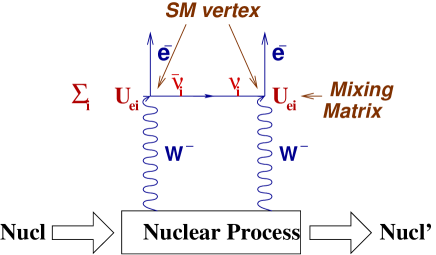
Figure 2: Diagram describing the double beta decay

The theoretically appealing option of Majorana neutrinos has been the object of extensive experimental programs and is under investigation by experiments both in run or in construction.

No clear evidence for this process has been observed at the moment, even though a claim of observation has been made with a mass of $0.4~{}\mathrm{eV}/\mathrm{c}^{2}$ [25]. Current upper limit on M_eff, affected by large uncertainties due to the nuclear matrix elements involved, is of the order of $1~{}\mathrm{eV}/\mathrm{c}^{2}$ [26].

For a review of the present experimental situation and future programs see reference [26].

As it will be shown in Section 3 oscillations can provide information only on the differences of square masses of neutrinos and not on their masses. Attempts to measure directly neutrino masses have given up to now only upper limits [27]:

• $m(\nu_{e})$ limits are obtained from the end point of the electron spectrum from Tritium decay, $m(\nu_{e})~{}\leq 2~{}\mathrm{eV}/\mathrm{c}^{2}$

• $m(\nu_{\mu})$ limits from the muon momentum end point in the $\pi$ decay,

  $m(\nu_{\mu})\leq~{}190~{}\mathrm{KeV}/\mathrm{c}^{2}$

• $m(\nu_{\tau})$ limits from the missing momentum of the 5 body semileptonic decay of $\tau$, $m(\nu_{\tau})\leq~{}18~{}\mathrm{MeV}/\mathrm{c}^{2}$.

A limit on the neutrino mass can also be derived from cosmological considerations, m$\leq$0.13 eV [28].

3 Neutrino oscillations

3.1 Vacuum oscillations

3.1.1 Three flavor mixing

In analogy to what happens in the quark sector the weak interaction states, called flavor eigenstates, $\nu_{e}$, $\nu_{\mu}$, $\nu_{\tau}$  are a linear combination of the mass eigenstates  $\nu_{1},\nu_{2},\nu_{3}$  that describe the propagation of the neutrino field. These states are connected by an unitary matrix U

$$\nu_{\alpha}=\sum_{j}U_{\alpha j}\cdot\nu_{j}$$

with index $\alpha$ running over the three flavor eigenstates and index j running over the three mass eigenstates. The $3\times 3$ matrix U is called the Pontecorvo–Maki–Nakagava–Sakata and is analogous to the Cabibbo–Kobaiashi–Maskawa (CKM) matrix in the quark sector.

In the general case a $3\times 3$ matrix can be parametrized by 3 mixing angles $\theta_{1}=\theta_{12}$, $\theta_{2}=\theta_{23}$, $\theta_{3}=\theta_{13}$ and a CP violating phase $\delta$

A frequently used parametrization of the U matrix is the following

$$U = \begin{pmatrix}1&0&0\cr 0&c_{23}&s_{23}\cr 0&-s_{23}&c_{23}\end{pmatrix}\begin{pmatrix}c_{13}&0&s_{13}e^{-i\delta}&\cr 0&1&0\cr-s_{13}e^{+i\delta}&0&c_{13}\end{pmatrix}\begin{pmatrix}c_{12}&s_{12}&0\cr-s_{12}&c_{12}&0\cr 0&0&1\end{pmatrix}$$ (1)

where $c_{jk}=\cos(\theta_{jk})$    and      $s_{jk}=\sin(\theta_{jk})$.

The factorized form of the matrix turns out to be very useful in data interpretation since the first matrix contains the parameters relevant for atmospheric and accelerator neutrino oscillations, the second one the parameters accessible to short distance reactor experiments and the CP violating phase $\delta$, while the third depends upon the parameters involved in solar neutrino oscillations.

Given three neutrino masses we can define two independent square mass differences $\Delta m^{2}_{12}$ and $\Delta m^{2}_{23}$.

As it will be shown in next sections $|\Delta m^{2}_{12}|\ll|\Delta m^{2}_{23}|$ and so $\Delta m^{2}_{13}\simeq\Delta m^{2}_{23}$.

The mass spectrum is formed by a doublet closely spaced $\nu_{1}$ and $\nu_{2}$, and by a third state $\nu_{3}$ relatively distant. This state can be heavier (normal hierarchy) or lighter (inverted hierarchy) ( $\Delta m^{2}_{23}$ positive or negative), the situation is depicted in Figure 3. Results discussed in Section 6 indicate that $\Delta m^{2}_{12}\approx 10^{-4}$ eV² and $\Delta m^{2}_{23}\approx 10^{-3}$ eV².

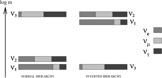
Figure 3: The two possible mass spectra for normal and inverted hierarchies.

3.1.2 The two flavor mixing

The mechanism of oscillations can be explained easily by using as an example the mixing between two flavor states and two mass states $m_{1}$ and $m_{2}$. The mixing matrix is reduced to $2\times 2$ and is characterized by a single parameter, omitting irrelevant phase factors:

$$\begin{pmatrix}\cos\theta&\sin\theta\\ -\sin\theta&\cos\theta\end{pmatrix}\quad$$

For the time evolution of a neutrino created for example as $\nu_{e}$ with a momentum p at time t=0 we can write (with the $\hbar$=c=1 choice of units)

$|\nu(0)>=|\nu_{e}>=\cos\theta|\nu_{1}>+\sin\theta|\nu_{2}>$

$|\nu(t)>=\cos\theta e^{-iE_{1}t}|\nu_{1}>+\sin\theta e^{-iE_{2}t}|\nu_{2}>$

where$E_{i}=\sqrt{p^{2}+m_{i}^{2}}$.

At a distance L $\approx$ t from the source the probability of detecting it in a different flavor, for example as a $\nu_{\mu}$, is

$$P(\nu_{e}\rightarrow\nu_{\mu})=|<\nu_{\mu}|\nu(t)>|^{2}=\sin^{2}(2\theta)\sin^{2}(\Delta M^{2}L/4E)$$

where $\Delta m^{2}=m_{1}^{2}-m_{2}^{2}$. Choosing to express $\Delta m^{2}$ in $eV^{2}$, L in meters and E in MeV (or in km and GeV respectively)

$$P(\nu_{e}\rightarrow\nu_{\mu})=\sin^{2}(2\theta)\sin^{2}(1.27\Delta M^{2}L/E)$$

In the two flavor scheme the survival probability for $\nu_{e}$ is given by

$$P(\nu_{e}\rightarrow\nu_{e})~{}~{}=1-P(\nu_{e}\rightarrow\nu_{\mu}).$$

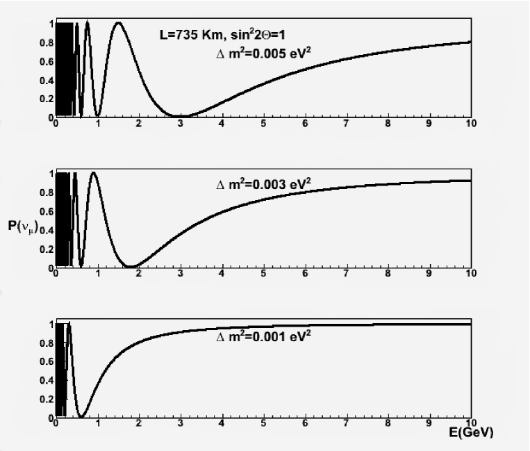
Figure 4: Oscillating behavior

We can define the oscillation length as ($\hbar$=c=1)

$$L_{osc}=4\pi E/\Delta m^{2}$$

that, adopting the units above, can be rewritten as

$$L_{osc}=2.48E/\Delta m^{2}$$

and so

$$P=\sin^{2}(2\theta)\sin^{2}(\pi L/L_{osc})~{}~{}$$

The oscillation probability has an oscillating behavior with the first maximum at  $L/L_{osc}=1/2$. Figure 4 shows examples of oscillation patterns as a function of the neutrino energy for fixed L and different values of $\Delta m^{2}$.

It should be noted that in the two flavor approximation CP and T violating terms vanish and

$$P(\nu_{\alpha}\rightarrow\nu_{\beta})=P(\nu_{\beta}\rightarrow\nu_{\alpha})$$

$$P(\nu_{\alpha}\rightarrow\nu_{\beta})=P(\overline{\nu}_{\alpha}\rightarrow\overline{\nu}_{\beta})$$

3.2 Matter oscillations

In the previous section it has been assumed that neutrinos propagate in vacuum. The presence of matter modifies the oscillation probability because one must include the amplitude for forward elastic scattering.

The scattering processes can be expressed in terms of a refraction index different for $\nu_{e}$ and $\nu_{\mu}$ or $\nu_{\tau}$. The difference in refraction index can then introduce additional phase shifts thus modifying the oscillation probability via the Mikheyev-Smirnov-Wolfenstein (MSW) effect [29, 30].

Let us define the effective potentials experienced by neutrinos in matter

$$V_{\mu,\tau}=\pm\sqrt{2}G_{F}(-N_{e}/2+N_{p}/2-N_{n}/2)$$

$$V_{e}=\pm\sqrt{2}G_{F}(-N_{e}/2+N_{p}/2-N_{n}/2+N_{e})$$

where the sign plus is for neutrinos and the sign minus for anti-neutrinos. $G_{F}$ is the Fermi coupling constant, N_e, N_p and N_n are the electron, the proton and the neutron number density. The additional term in the second equation arises from the W exchange contribution to the scattering process $\nu_{e}+e\rightarrow\nu_{e}+e$ (see Section 5.2).

The relevant quantity for neutrino propagation is $\Delta V_{e,\alpha}=V_{e}-V_{\alpha}$, the difference between potentials for electron neutrinos and neutrinos of flavor $\alpha$ ($\alpha=\mu$ or $\tau$).

$$\Delta V_{e,\alpha}=\pm\sqrt{2}G_{F}\cdot N_{e}={\pm}7.6\cdot 10^{-14}~{}eV\cdot\rho\cdot(Z/A)$$

where $\rho$ is the density of matter (in g/cm³). Defining $B=2E\Delta V$, $\epsilon=B/\Delta m^{2}$, assuming a constant density (a reasonable assumption for terrestrial long baseline experiments), in the two flavor mixing treatment we can replace vacuum parameters with matter parameters

$$\sin 2\theta_{m}=\sin 2\theta/\sqrt{(\cos 2\theta-\epsilon)^{2}+\sin^{2}2\theta}$$

$$\Delta m^{2}_{m}=\Delta m^{2}\sqrt{(\cos 2\theta-\epsilon)^{2}+\sin^{2}2\theta}$$

$\epsilon$ sign is positive for neutrinos and a positive $\Delta m^{2}$ value, and is reverted for anti-neutrinos or for negative $\Delta m^{2}$.

The oscillation probability can be written as

$$P=\sin^{2}(2\theta_{m})\sin^{2}(\Delta m^{2}_{m}L/4E)$$

In the limit $\epsilon\ll\cos 2\theta$ matter effects become negligible.

The above formulas are valid in the case of propagation in a constant density medium, variable density becomes important in the propagation of neutrinos in the Sun, treatment of this situation can be found in [31].

The treatment of matter effects in the three flavor case is complicated and can be found in [32].

3.3 Approximations for the oscillation probabilities

The oscillation probability in the 3 flavor case contains two mass differences, three mixing angles, the phase $\delta$ and the matter effect contribution. Approximate formulas in terms of $\alpha=\Delta m^{2}_{12}/\Delta m^{2}_{23}$ and in terms of the mass effect term B, have been developed in the limit $\alpha\ll 1$ and $B/\Delta m^{2}_{23}\ll 1$ [33, 34, 35, 36].

For example, for the $\nu_{\mu}\rightarrow\nu_{e}$ oscillation probability has been written in ref [35] as :

$$P(\nu_{\mu}\rightarrow\nu_{e})=sin^{2}\theta_{23}sin^{2}2\theta_{13}{{sin^{2}[(1-A)\Delta]}\over{(1-A)^{2}}}$$

$$\pm J\alpha sin\delta_{CP}sin{\Delta}{{sin(A\Delta)}\over{A}}{{sin[(1-A)\Delta]}\over{(1-A)}}$$

$$+J\alpha cos\delta_{CP}cos{\Delta}{{sin(A\Delta)}\over{A}}{{sin[(1-A)\Delta]}\over{(1-A)}}$$

$$+\alpha^{2}cos^{2}\theta_{23}sin^{2}2\theta_{12}{{sin^{2}(A\Delta)}\over{A^{2}}}$$

(2)

Where J=$cos\theta_{13}sin2\theta_{12}sin2\theta_{13}sin2\theta_{23}$

$\alpha=\Delta m^{2}_{12}/\Delta m^{2}_{23},\Delta=\Delta m^{2}_{23}L/4E,A=B/\Delta m^{2}_{23}$, B as defined in Section 3.2.

The appearance probability, neglecting matter effects, for accelerator neutrinos in the 3 flavor mixing scheme using $\Delta m^{2}_{12}=8\times 10^{-5}~{}\mathrm{eV}^{2}$ ($\alpha\approx 0$), and $L/E\simeq$  1 and therefore $\sin^{2}(\Delta m^{2}_{12}L/4E)\simeq 0$ is:

$$P(\nu_{\mu}\rightarrow\nu_{e})=\sin^{2}(2\theta_{13})\sin^{2}(\theta_{23})\sin^{2}(\Delta m^{2}_{23}L/4E)$$

It can be shown that in the same approximation:

$$P(\nu_{\mu}\rightarrow\nu_{\tau})=\cos^{4}(\theta_{13})\sin^{2}(2\theta_{23})\sin^{2}(\Delta m^{2}_{23}L/4E)$$

$$P(\nu_{e}\rightarrow\nu_{\tau})=\sin^{2}(2\theta_{13})\cos^{2}(\theta_{23})\sin^{2}(\Delta m^{2}_{23}L/4E)$$

For $\sin^{2}(2\theta_{13})\simeq 0$ the only probability different from 0 is $P(\nu_{\mu}\rightarrow\nu_{\tau})$ that can be written as

$$P(\nu_{\mu}\rightarrow\nu_{\tau})=\sin^{2}(2\theta_{23})\sin^{2}(\Delta m^{2}_{23}L/4E)$$

depending upon two parameters $\theta_{23}$ and $\Delta m^{2}_{23}$ that will coincide with the two parameters of the simplified treatment.

In this approximation the $\nu_{\mu}$ survival probability in atmospheric or accelerators neutrino experiments will be given by $1-P(\nu_{\mu}\rightarrow\nu_{\tau})$.

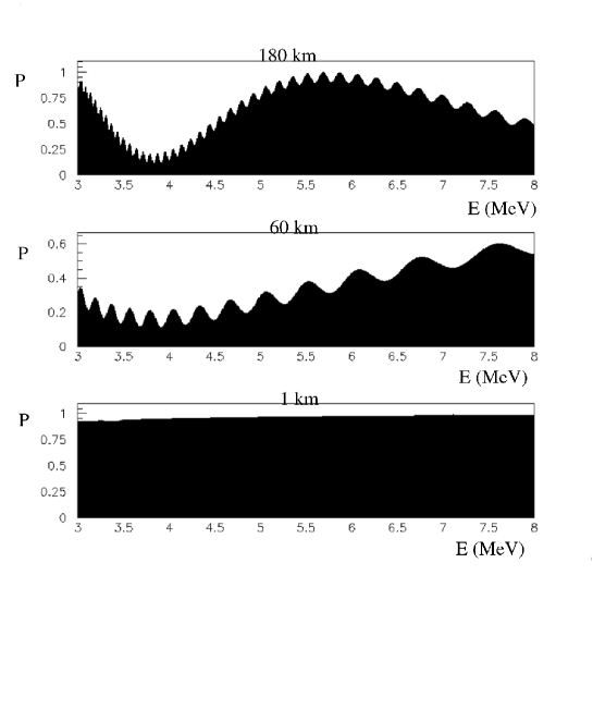
Figure 5: Probability for $P(\overline{\nu}_{e}\rightarrow\overline{\nu}_{e})$ versus neutrino energy (in MeV) at L = 180, 60, 1 km from the source.

In reactor experiments(see section 6.2), in which matter effect can be neglected because the energy and matter density involved are small, the survival probability of a $\overline{\nu}_{e}$ will be given by

$$P(\overline{\nu}_{e}\rightarrow\overline{\nu}_{e})=1-P1-P2$$

with

$$P1=\cos^{4}(\theta_{13})\sin^{2}(2\theta_{12})\sin^{2}(\Delta m^{2}_{12}L/4E)$$

$$P2=\sin^{2}(2\theta_{13})\sin^{2}(\Delta m^{2}_{23}L/4E)$$

At short distances $\sin^{2}(\Delta m^{2}_{12}L/4E)\simeq 0$ and the term P1 can be neglected.

$$P(\overline{\nu}_{e}\rightarrow\overline{\nu}_{e})=1-P2=1-\sin^{2}(2\theta_{13})sin^{2}(\Delta m^{2}_{23}L/4E)$$ (3)

will be sensitive to $\theta_{13}$  and   $\Delta m^{2}_{23}$.

At large distances the term P1 will be dominant and in the limit of $\sin^{2}(2\theta_{13})\simeq 0$ we will have

$$P(\overline{\nu}_{e}\rightarrow\overline{\nu}_{e})=1-P1=1-\cos^{4}(\theta_{13})\sin^{2}(2\theta_{12})\sin^{2}(\Delta m^{2}_{12}L/4E).$$

Figure 5 shows $P(\overline{\nu}_{e}\rightarrow\overline{\nu}_{e})$ as a function of the neutrino energy for E($\nu$)=3-8 MeV (typical of reactor neutrinos), L=180, 60, 1 km and with $\sin(2\theta_{13})=0.05$, $\sin(2\theta_{12})=0.314$, $\Delta m^{2}_{12}=7.9\times 10^{-5}eV^{2}$,$\Delta m^{2}_{23}=2.5\times 10^{-3}eV^{2}$.

3.4 Experimental determination of neutrino oscillation parameters

Table 1 gives the $\Delta m^{2}$ values accessible to different neutrino sources according to $\Delta m^{2}\approx E/L$.

Neutrino source	Distance from source (Km)	Energy (GeV)	$\Delta m^{2}$ (eV2)
solar	$10^{8}$	$10^{-3}$	$10^{-11}$
atmospheric from top	20	1,10	$0.05,0.5$
atmospheric from bottom	$10^{4}$	1,10	$10^{-4}$, $10^{-3}$
reactors	1	$10^{-3}$	$10^{-3}$
reactors large distance	100	$10^{-3}$	$10^{-5}$
accelerators	1	1,20	1,20
accelerators long distance	100,1000	1,20	$10^{-3},0.2$

Table 1: Sensitivity to $\Delta m^{2}$ of experiments studying different neutrino sources

In the two flavor scheme the determination of the oscillation probability P gives a relation between $\Delta m^{2}$and $\sin^{2}(2\theta)$ in the ($\Delta m^{2}$,$\sin^{2}(2\theta)$) plane. A measurement of P gives a region in the parameter plane whose extension depends on the resolution of the oscillation probability measurement. In the case of a negative result an exclusion region can be drawn. Examples of the two cases are shown in Figure 6.

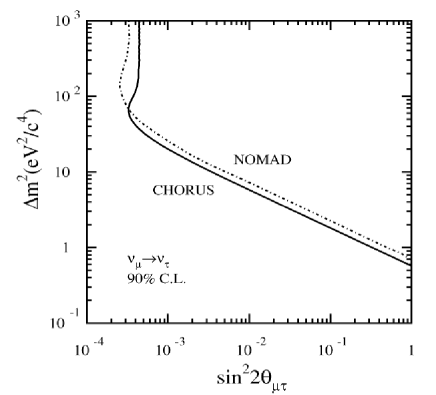
Figure 6: Experimental results represented in the ($\Delta m^{2}$, $\sin^{2}(2\theta)$) plane: for positive (A), figure from ref. [37], and negative (B), from ref. [38], copyright (2008), with permission from Elsevier (results also from ref. [39]).

Oscillations can be studied in two different approaches by the so-called disappearance and appearance experiments.

3.4.1 Disappearance experiments

The flux of neutrinos of a given flavor $\nu_{\alpha}$ at a distance L from the source, $\Phi(L)$, is compared to the flux at the source, $\Phi(0)$. The ratio $\Phi(L)/\Phi(0)$ will give the survival probability of the neutrino, but no information on the type of neutrino to which $\nu_{\alpha}$ has oscillated. These experiments crucially depend upon the knowledge of $\Phi(0)$. This approach is the only possible one for the low energy $\nu_{e}$ or $\overline{\nu}_{e}$ (solar or reactor neutrinos) since CC interactions of $\nu_{\mu}$ or $\nu_{\tau}$ are kinematically forbidden.

The uncertainties related to the knowledge of $\Phi(0)$ can be canceled measuring the ratio of fluxes measured by two detectors positioned at distances L (far detector) and $l\ll$L (near detector) from the source.

3.4.2 Appearance experiments

Starting with a source of $\nu_{\alpha}$, flavor $\nu_{\beta}$ neutrinos will be searched for at a distance L. In these experiments the main source of systematic errors are the contamination from $\nu_{\beta}$ at the production point and background mistaken as $\nu_{\beta}$ CC interactions. Typical examples of this approach are experiments with accelerators producing $\nu_{\mu}$ neutrino beams. These $\nu_{\mu}$ beams have a small contamination of $\nu_{e}$. So in a search for $\nu_{\mu}\rightarrow\nu_{e}$ oscillation a possible signal must be extracted from the contribution of beam $\nu_{e}$.

The following general considerations can be made

• the smallness of cross sections requires large mass targets in order to have an appreciable number of interactions. In general, target and detector coincide, both in appearance and disappearance experiments.

• appearance experiments require the determination of the flavor of the involved neutrinos. The detection of flavor does not give problems in the case of $\nu_{\mu}$, while the detection of $\nu_{e}$ can give problems at high energies, where electromagnetic showers from gamma coming from $\pi^{0}$ decays can mimic electrons. The detection of $\tau$ is made difficult by the short lifetime of this particles. $\nu_{\mu}$ and $\nu_{\tau}$ can of course be identified only above the energy threshold for Charged Current interactions.

4 Neutrino sources

4.1 Solar neutrinos

Neutrinos are produced in the thermonuclear reactions that take place in the Sun core. The process is initiated by the reactions par

$$p+p\rightarrow H^{2}+e^{+}+\nu_{e}$$

$$p+e^{-}+p\rightarrow H^{2}+\nu_{e}$$

followed by a chain of processes illustrated in Table 2, whose net result is

$$4p+2e^{-}\rightarrow He^{4}+2\nu_{e}+\gamma.$$

Another source of neutrinos is the CNO Cycle, whose contribution to the solar neutrino flux is negligible [40].

Reaction	$\%$ of terminations	neutrino energy (MeV)
$p+p\rightarrow H^{2}+e^{+}+\nu$	(99.75)	0-0.420
$p+e^{-}+p\rightarrow H^{2}+\nu$	(0.25)	1.44
$H^{2}+p\rightarrow He^{3}+\gamma$	(100)
$He^{3}+He^{3}\rightarrow He^{4}+2p$	(86)
OR
$He^{3}+He^{4}\rightarrow Be^{7}+\gamma$
$Be^{7}+e^{-}\rightarrow Li^{7}+\nu$	(14)	0.861 (90$\%$), 0.383 (10$\%$)
$Li^{7}+p\rightarrow 2He^{4}$
OR
$Be^{7}+p\rightarrow B^{8}+\gamma$
$B^{8}\rightarrow(Be^{8})^{*}+e^{+}+\nu$	(0.015)	14.06
$(Be^{8})^{*}\rightarrow 2He^{4}$

Table 2: pp chain in Sun, from reference [41]

The Q value of the reaction is 26 MeV and the corresponding energy is released mainly in the form of electromagnetic radiation. The average energy of the emitted neutrinos is $\approx$ 0.5 MeV.

The computation of the rate of these processes has been initiated by Bahcall in the sixties and his more recent evaluation, using different models for Sun parameters, has been published in reference [42].

The contribution from the pp cycle is very well determined and constitutes $\approx 99\%$ of the solar neutrino flux on earth. Figure 7 shows the energy distribution of the different sources of solar neutrinos. The information is summarized in Table 3.

Figure 7: Spectra of neutrinos from different processes in the Sun [42]. reproduced by permission of the AAS.

process	flux	error	mean energy	energy max
	$10^{10}~{}cm^{-2}s^{-1}$	$\%$	MeV	MeV
pp	6.0	1.	0.267	0.42
pep	1.4 x$10^{-2}$	1.5	1.44	1.44
hep	7.6x$10^{-7}$	15	9.68	18.8
Be7	4.7x$10^{-1}$	10	0.81	0.87
B8	5.8x$10^{-4}$	16.	6.73	14.0
N13	6.1x$10^{-2}$	30.	0.70	1.2
O15	5.2x$10^{-2}$	30	0.99	1.73

Table 3: Rates of neutrino fluxes from the Sun  [42] with error estimates from [43].

The error column in Table 3 shows that the Standard Solar Model (SSM) predicts with high precision the rate of the pp fusion, which also produces most of the neutrino flux on earth. The flux for pp neutrinos is predicted with a small error and so deviation from these predictions are a strong indication of oscillations. The final confirmation of the SSM has been given by the SNO experiment, which found the total all neutrino flavours flux (above 5 MeV) in agreement with the model prediction (see section 6.1.2).

The different techniques used in solar neutrino detectors have different energy thresholds, so they are sensitive to different components of the solar neutrino spectrum. The threshold for Chlorine detectors [1] is 0.814 MeV, well above the end point of the neutrino energy in the pp process, while Gallium detectors [44] have a threshold at 0.233 MeV which makes them sensitive to pp neutrinos. For water counters [7] the energy threshold is fixed by the minimum electron energy that can be detected above background (few MeV).

4.2 Reactor neutrinos

Nuclear reactors are an intense source of $\overline{\nu}_{e}$, generated in the beta decay of fission fragments produced in the fission. Each fission releases about 200 MeV and 6 $\overline{\nu}_{e}$. The average energy of $\overline{\nu}_{e}$ is of the order of few MeV, well below the $\mu$ and $\tau$ production thresholds in CC interactions, therefore only disappearance experiments are possible. These experiments require the flux and the energy spectrum of neutrinos to be known with great precision.

Neutrinos are detected through the reaction $\overline{\nu}_{e}+p=e^{+}+n$ which has a threshold at 1.8 MeV.

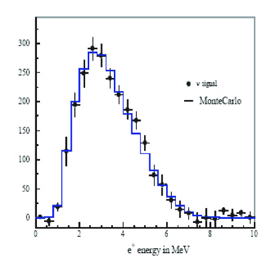
Figure 8: Example of energy spectrum of positrons produced in reactor neutrinos interactions, showing the level of accuracy of flux predictions. Figure from [45], with kind permission of the European Physical Journal (EPJ).

The determination of the neutrino flux is based upon the knowledge of the thermal power of the reactor core and of the fission rate of the relevant isotopes $U^{235},~{}U^{238},~{}Pu^{239},~{}Pu^{241}$. The $\beta$ spectrum of the fission fragments is then converted in the $\overline{\nu}_{e}$ spectrum, which can be predicted at the $10^{-2}$ level. The agreement of predictions and data is demonstrated in Figure 8 where the measured positron spectrum in the CHOOZ detector is compared to Monte Carlo prediction [45].

4.3 Atmospheric neutrinos

Atmospheric neutrinos are generated by the interaction of primary cosmic ray radiation (mainly protons) in the upper part of the atmosphere. The average distance traveled by pions and kaons before decay $\gamma c\tau$ (with $c\tau=7.8~{}m$ for pions and $c\tau=3.7~{}m$ for kaons) is such that they decay in flight, while some of the muons produced in their decay ($c\tau=658~{}m$) reach earth undecayed. Neutrinos and anti-neutrinos are produced in the processes

$$\pi^{+}\rightarrow\mu^{+}+\nu_{\mu}$$

$$\pi^{-}\rightarrow\mu^{-}+\overline{\nu}_{\mu}$$

$$K^{+}\rightarrow\mu^{+}+\nu_{\mu}+X$$

$$K^{-}\rightarrow\mu^{-}+\overline{\nu}_{\mu}+X$$

$$\mu^{+}\rightarrow e^{+}+\overline{\nu}_{\mu}+\nu_{e}$$

$$\mu^{-}\rightarrow e^{-}+\nu_{\mu}+\overline{\nu}_{e}$$

One of the most recent flux computations has been made by Honda and collaborators  [46], who also provide references to previous computations.

If all the muons could decay the ratio $\nu_{\mu}/\nu_{e}$ would be 2. This ratio is larger at high energies as shown by the energy spectra of atmospheric neutrinos in Figure 9, in which results of Honda’s computation are compared to those of other models.

Figure 9: Atmospheric neutrino fluxes and the ratio $\nu_{\mu}/\nu_{e}$. Figure from reference  [47], copyright (2004) by the American Physical Society. Solid line Honda et al. [47], dotted line Honda et al. [48], dashed line Fluka group [49, 50] long dashed Agrawal et al. [51].

The neutrino flux for $E\approx 1$ GeV is $\approx 0.1m^{-2}s^{-1}$ and is up-down symmetric.

4.4 Accelerator neutrinos

Neutrino beams are produced by proton accelerators. The extracted proton beam interacts on a target and the produced particles are focused by a magnetic system (horn) whose polarity selects the desired charge of the particles. Pions (and kaons) are allowed to decay in an evacuated tunnel followed by an absorber stopping all particles except neutrinos and anti-neutrinos. The resulting beam contains mainly $\nu_{\mu}$ ($\overline{\nu}_{\mu}$) when positive (negative) particles are focused. A small contamination of $\overline{\nu}_{\mu}$ ($\nu_{\mu}$) and $\nu_{e}$ ($\overline{\nu}_{e}$) is due at high energy to the kaon semileptonic decay $K^{+}\rightarrow\pi^{0}+e^{+}+\nu_{e}$, while at low energy there is a contamination from muon decay. A schematic drawing of the CERN Wide Band Neutrino Beam (WBB) from the SPS is shown in Figure 10. It is a typical high energy $\nu_{\mu}$ beam (a similar beam has been built at FNAL) whose composition is given in Table 4. The momentum distribution of the neutrino produced is shown in Figure 11.

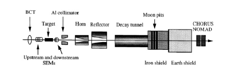
Figure 10: schematic view of a neutrino beam. Figure from  [52]

This beam has been used for several neutrino experiments CDHS [53], CHARM [54], CHARM2 [55] and in the oscillation search for $\nu_{\mu}\rightarrow\nu_{\tau}$ by the CHORUS [56] and NOMAD [57] experiments.

Figure 11: Neutrino fluxes in the CERN WBB beam from reference [58].

neutrinos	relative abundance	average energy (GeV)
$\nu_{\mu}$	1.	24.3
$\overline{\nu}_{\mu}$	0.0678	17.2
$\nu_{e}$	0.0102	36.4
$\overline{\nu}_{e}$	0.0027	27.6

Table 4: Composition of the WBB beam at the CERN SPS from reference [58].

The relative abundance of $\nu_{\tau}$ has been extimated of the order of $10^{-6}$ (see for example ref [56])

The neutrino energy is correlated to the momentum of the protons. Figure  12 shows the momentum spectrum of neutrino produced by 19 GeV protons extracted from the CERN PS. This beam has been used from the CDHS [59], CHARM [60] and BEBC (The Big European Bubble Chamber) [61] for neutrino oscillation searches.

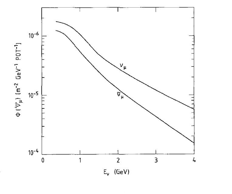
Figure 12: Neutrino fluxes in the medium energy CERN PS beam. From reference [60], copyright (1984), with permission from Elsevier.

The discovery of $\nu_{\mu}$ oscillation in the $\Delta m^{2}\approx 10^{-3}~{}\mathrm{eV}^{2}$ region has pushed for low energy beams and long distance experiments ($\Delta m^{2}\approx E/L$). The energy spectrum of the neutrino beam from the 12 GeV protons of the KEK proton synchrotron at the K2K[14] near detector is shown in Figure 13. Figure 14 shows the spectrum for the NUMI beam from the 120 GeV main injector at Fermilab, used for MINOS [62], in three different possible configurations.

Figure 13: The K2K beam, from from reference [14], copyright (2006) by the American Physical Society.

Figure 14: The NUMI beam: spectra in the low, medium and high energy beam configurations, from reference [37].

Off axis beams have also been designed to meet the need of low energy beams of well defined energy. They were first proposed by the E889 [63] collaboration in 1995. If neutrinos are observed at an angle with respect to the incoming proton beam, thanks to the kinematical characteristics of the two body decay, the neutrino energy becomes almost independent from the pion energy

$$E_{\nu}=0.43\cdot E_{\pi}/(1+\gamma_{\pi}^{2}\cdot\theta_{\pi\nu}^{2})$$

with $\gamma_{\pi}=E_{\pi}/m_{\pi}$. Figure 15 shows the neutrino energy as a function of the pion energy for different angles. Detecting the neutrinos off axis has the advantage of giving a relatively well defined momentum and of cutting the high energy part of the spectrum, see for example Figure 44.

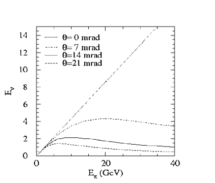
Figure 15: The off axis beam: neutrino energy as a function of the pion energy for neutrinos produced at an angle $\theta$ relative to the pion beam direction,from reference [64].

A completely different approach has been used in the production of anti-neutrinos for the LSND experiment [65]. Low energy protons (0.8 GeV) interacting in an absorber produce low energy pions. The decay $\pi^{+}\rightarrow\mu^{+}+\nu_{\mu}$ is followed by the  $\mu^{+}\rightarrow e^{+}+\overline{\nu}_{\mu}+\nu_{e}$ one. $\pi^{-}$ are absorbed when they stop, a small fraction can decay in flight, in this case their decay muons come at rest and then can absorbed or decay. An isotropic source of neutrinos is produced, mainly $\nu_{\mu}$, $\overline{\nu}_{\mu}$, $\nu_{e}$ and a small fraction of $\overline{\nu}_{e}$ coming from the decay $\mu^{-}\rightarrow e^{-}+\nu_{\mu}+\overline{\nu}_{e}$. These $\overline{\nu}_{e}$ will be the main source of background in the search of the oscillation $\overline{\nu}_{\mu}\rightarrow\overline{\nu}_{e}$.

5 Neutrino interactions

This section will be devoted to the neutrino interactions that play a key role in the oscillation experiments. When the oscillations are revealed by the presence of a certain flavor in the final state, only charged current interactions (CC) are relevant. Neutral current interactions (NC) are used when the total flux of neutrinos, regardless of their flavor, is measured.

5.1 Neutrino-nucleon scattering

a) Energies E($\nu$)$\approx$ 1-10 MeV (solar and reactor neutrinos)

At these energies $\nu_{e}$ and $\overline{\nu}_{e}$ can experience charged current reactions only by scattering on free, (quasi)-free nucleons

$\overline{\nu}_{e}+p\rightarrow e^{+}+n$

$\nu_{e}+n\rightarrow e^{-}+p$
The cross section of the first process has a threshold at 1.8 MeV, in fact the positron kinetic energy is given by

$$T(e^{+})=E(\overline{\nu}_{e})+M(p)-M(n)-M(e)=E(\overline{\nu}_{e})-1.8~{}\mathrm{MeV}$$

b) Scattering at medium energy E($\nu$) $\simeq$ 1 GeV (atmospheric and accelerator neutrinos)

Above the threshold for muon production the quasi elastic CC processes start

$\overline{\nu_{\mu}}+p=\mu^{+}+n$

$\nu_{\mu}+n=\mu^{-}+p$

followed by $\pi^{0}$ or charged $\pi$ production via resonances and by deep inelastic processes at higher thresholds.

Figure 16: Charged current total cross section from reference  [14], copyright (2006) by the American Physical Society, divided by $E_{\nu}$ for neutrino nucleon charged current interactions. The solid line shows the calculated total cross section. The dashed, dot and dash-dotted lines show the calculated quasi-elastic, single-meson and deep-inelastic scattering, respectively. The data points are taken from the following experiments: ($\triangle$)ANL[66], ($\bigcirc$)GGM77[67], ($\bullet$)GGM79(a)[68],(b)[69], ($\ast$)Serpukhov[70], ($\Diamond$)ANL82[71], ($\star$)BNL86[72], ($\blacksquare$)CCFR90[73], ($\blacktriangledown$)CDHSW87[74], ($\times$)IHEP-JINR96[75], ($+$)IHEP-ITEP79[76], ($\Box$)CCFRR84[77], and ($\blacktriangle$)BNL82[78].

Figure 16, from reference [14], shows experimental measurements of neutrino cross section together with the calculated value as a function of the neutrino energy.

c) High energy E($\nu$) $\gg$ 1 GeV (accelerator neutrinos)

The deep inelastic scattering on quarks dominates at high energy. Cross sections for $\nu_{e}$ and $\nu_{\mu}$ are

$\sigma(\nu)=0.67~{}10^{-38}cm^{2}E_{\nu}/\mathrm{GeV}$, for neutrinos

$\sigma(\overline{\nu})=0.34~{}10^{-38}cm^{2}E_{\nu}/\mathrm{GeV}$, for anti-neutrinos.

For $\nu_{\tau}$ the high mass of the $\tau$ lepton modifies the threshold of the various processes and changes also the cross section at higher energies. The linear growth with E_ν of the cross section continues until the effect of the propagator becomes important.

5.2 Neutrino-electron scattering

The scattering of neutrinos on electrons is a purely weak process which is different for $\nu_{e}$ and other neutrinos. In fact both CC and NC contribute to the $\nu_{e}$ cross section while for $\nu_{\mu}$ and $\nu_{\tau}$ only NC processes are possible (see Figure 17). Again the cross sections depend linearly upon E_ν:

$$\sigma(\nu_{e})=0.93~{}10^{-41}cm^{2}E_{\nu}/\mathrm{GeV}$$

$$\sigma(\nu_{\mu},\nu_{\tau})=0.16~{}10^{-41}cm^{2}E_{\nu}/\mathrm{GeV}$$

and the ratio of the cross sections is

$$\frac{\sigma(\nu_{e})}{\sigma(\nu_{\mu}~{}or~{}\nu_{\tau})}\approx~{}6$$

Figure 17: neutrino electron scattering

The following characteristics of $\nu$ scattering on electrons must be noted: due to the small mass of the electron

a) cross sections of $\nu$ on electron at high energies are smaller by a factor $\simeq 10^{-3}$ compared to cross sections on nucleons. In fact cross sections are proportional to the mass of the scattering particle.

b) the electron will be emitted in the forward direction. The scattering angle $\theta$ of the electron in the laboratory system is such that $\theta^{2}\leq 2m_{e}/E$, where E is the energy of the electron.

Figure 18 compares the $\overline{\nu}_{e}$ charged current cross section for scattering on protons with the $\nu_{e}$ total cross section on electrons. For E_ν smaller than the mass m of the target the cross section is proportional to E${}_{\nu}^{2}$, while for E_ν larger than m the cross section is proportional to the product $mE_{\nu}$.

Figure 18: Neutrino cross sections vs energy for scattering on nucleon or electron, from reference [22].

5.3 Neutrino-nucleus scattering

At low energies the relevant reactions, exploited by radiochemical experiments, are

$$\nu_{e}+A(Z,N)\rightarrow e^{-}+A(Z+1,N)$$

$$\overline{\nu}_{e}+A(Z,N)\rightarrow e^{+}+A(Z-1,N)$$

The final nucleus is unstable and decays by electron capture. In the rearrangement of atomic electrons that follows electron capture, a photon or Auger electron is emitted.

Cross sections for these processes can be found in reference [79].

6 Experimental results

This section summarizes the results obtained in the neutrino oscillation field using neutrinos both from natural and artificial sources.

6.1 Solar neutrinos

The pioneering experiment of R. Davis did start the ’solar neutrino puzzle’: solar neutrinos observed on the earth are a fraction of those predicted by the Solar Standard Model (SSM). The first results were published by Davis in 1968 [1] but only in 2002 the dilemma ”problem with the neutrino” or ”problem with SSM” was solved by the SNO results. Indeed Davis had observed neutrino oscillations. In the following, we will give a brief account of the different experiments dedicated to the detection of solar neutrinos, which are divided into two categories: radiochemical experiments and real time experiments.

6.1.1 Radiochemical experiments:

In radiochemical experiment the $\nu_{e}$ from the sun interact with a nucleus via the reaction

$$\nu_{e}+A1(Z,A)\rightarrow e^{-}+A2(Z+1,A)$$

where the transition A1 to A2 leads to an unstable nucleus. The rate of the reaction is measured by counting the number of A2 nuclei, detected via their decay.

The threshold of the previous reaction fixes the minimum energy of the solar neutrinos that can be detected.

The Chlorine experiment:

Following a suggestion of B.Pontecorvo, R. Davis started a neutrino experiment in the Homestake Gold mine in South Dakota, at a depth of 4800 meter water equivalent (MWE). After a test experiment performed in 1964 [80] showing that large underground experiment were feasible, Davis and collaborators proceeded to build a large container filled with 100000 gallons of tetrachloroetilene. The observed reaction was

$$\nu_{e}+Cl^{37}\rightarrow Ar^{37}+e^{-}$$

The cross section, integrated on the B⁸ spectrum, of this process has been computed to be (1.14$\pm$0.037)$\times 10^{-42}$ cm² [79]. In Davis’s experiment the rate of interactions is not measured directly. Using physical and chemical methods the amount of $Ar^{37}$ was extracted from the target material. The $Ar^{37}$ is unstable, the counting was performed by observing the Auger electron or photon emitted in the decay. Since the $Ar^{37}$ decay half-time is 35 days, the extraction had to be performed periodically, 1 run each 2 months.

The first indication of a neutrino deficit was given in 1968 [1]. Bahcall in the same year [81] did show that these results were incompatible with his calculations on the solar model.

The results, for runs taken from 1970 to 1995, give for the solar neutrino capture rate the value 2.56$\pm$ 0.16 stat $\pm$ 0.16 syst SNU [2] (1 SNU=$10^{-36}$neutrino captures/(atom sec)). This result corresponds to a reduction by a factor $\simeq$3 (Table 6) with respect to the prediction of the SSM, and represents the first evidence for neutrino oscillation.

Note that since the threshold of the reaction on $Cl^{37}$ is 0.813 MeV, this experiment is marginally sensitive to the $Be^{7}$ solar neutrinos, and mainly to the $B^{8}$ neutrinos.

Gallium experiments:

Three radiochemical experiments have studied solar neutrinos using the scattering on Gallium:

$$\nu_{e}+Ga^{71}\rightarrow Ge^{71}+e^{-}$$

Since the threshold of this reaction is 0.233 MeV Gallium experiments are sensitive to the neutrinos from the primary pp reaction in the sun. The three Gallium experiments are GALLEX [4] and its continuation GNO [5], at the Gran Sasso Laboratory in Italy, and SAGE [3], at the Baksan Neutrino Observatory in Russia. To ensure the correctness of the results all these detectors have been calibrated with strong neutrino sources.

GALLEX and GNO:

The GALLEX experiment [4] started data taking in 1991 at the Gran Sasso Laboratory, at a depth of 3500 MWE. It used a large tank to contain 30 tons of gallium dissolved in 100 tons aqueous gallium chlorine solution. The target material was periodically extracted to count the $Ge^{71}$ produced in the neutrino interaction. The amount of $Ge^{71}$ was measured by detecting its decay products, X rays or Auger electrons following electron capture, with proportional counters. Data were taken from 1991 to 1997.

GALLEX was followed by the GNO experiment [5], which took data from 1998 to 2003. GALLEX+GNO performed separate measurements of the solar neutrino flux for the 123 runs taken between 1991 and 2003. The time behavior of these measurements is shown in Figure 19, results are summarized in Table 5.

Figure 19: Results from GALLEX and GNO data taking,from reference  [5], copyright (2005), with permission from Elsevier.

SAGE Experiment:

The SAGE experiment [3] is located in the Baksan neutrino observatory 4700 MEW under the sea level. An average mass of 45.6 tons of metallic Gallium $Ga^{71}$ was used.

In the period 1990-2003 107 neutrino runs were taken and the result of their analysis is shown in Table 5.

GALLEX [4]	77.5 $\pm$ 6.2 ${}^{+4.3}_{-4.7}$
GNO [5]	62.9 ${}^{+5.5}_{-5.3}$$\pm$2.5
GNO+GALLEX [5]	69.3 $\pm$4.1
SAGE [3]	70.8 ${}^{+5.3}_{-5.2}$ ${}^{+3.7}_{-3.2}$

Table 5: Gallium experiments results, capture rates expressed in SNU

The weighted average of all Gallium results is [44]

$$Capture~{}Rate=67.6\pm 3.71~{}~{}SNU$$

which compared with a prediction of 128 SNU gives a Data/SSM ration of 0.53 (see Table 6).

6.1.2 Real time experiments:

Solar neutrinos have been studied in real time using huge water (Kamiokande [82] and Super-Kamiokande (SK) [6]) or heavy water (SNO [8]) containers surrounded by a very large number of photomultipliers used to detect the Cherenkov light emitted by fast particles produced in neutrino interactions. The Cherenkov threshold in water is $\beta$=0.75. The use of this technique to detect solar neutrinos as been pioneered by the Kamiokande experiment and by its follow-up Super-Kamiokande where the only reaction allowed for neutrinos of $E\simeq$ MeV is the scattering on electrons.

Two relevant characteristics of this process are

a) in the scattering on electrons take part not only $\nu_{e}$ but with a smaller cross section ( $\simeq$ 1/6) also $\nu_{\mu}$ and $\nu_{\tau}$;

b) the direction of scattered electrons is tightly connected with the direction of the incoming neutrino.

Figure 20 shows the angular distribution of observed electrons.

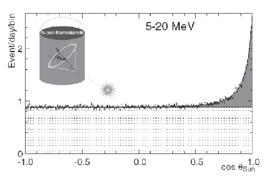
Figure 20: Angular distribution of observed electrons in Super-Kamiokande, from reference [7], copyright (2006) by the American Physical Society.

The SNO experiment (Sudbury Neutrino Observatory) [8] has allowed also the study of neutral current interactions and charged current interactions using the quasi-free neutrons of deuterium.

Kamiokande and Super-Kamiokande:

Kamiokande and Super-Kamiokande base their study on the detection of the neutrino scattering on electrons $\nu+e\rightarrow\nu+e$.

The Kamiokande [82] detector was originally built mainly to search for proton decay, it did start operation in 1983.

The detector consisted of a cylinder 16 m high, with 16.5 m diameter containing 3000 tons of pure water. The surface was equipped with 1000 photomultipliers of 50 cm diameter.

In water counters electrons are recognized by the characteristic Cherenkov ring. Figure 21 shows a few MeV electron ring.

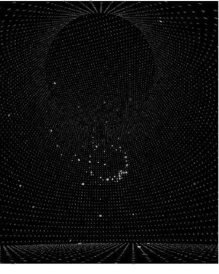
Figure 21: Cherenkov ring of a few MeV electron in the Super-Kamiokande detector, from http://www.ps.uci.edu/$\sim$tomba/sk/tscan/pictures.html

The energy threshold to reject background was fixed to 9.3 MeV and then lowered to 7 MeV during data taking. This threshold made the experiment sensitive only to $B^{8}$ neutrinos and 800 events were collected.

The result of the experiment was [6]

$$\Phi(\nu_{e})=(2.80\pm 0.19\pm 0.33)\times 10^{6}cm^{-2}sec^{-1}.$$

The ratio Data/SSM=0.55$\pm 0.04\pm 0.07$ confirmed the solar neutrino deficit.

The Kamiokande detector was followed by the Super-Kamiokande one.

A schematic drawing of the detector is shown in Figure 22.

Figure 22: Layout of the Super-Kamiokande detector, from reference  [83], copyright (2005) by the American Physical Society.

Construction started in 1991 and was completed in 1995. Data taking did start in 1996.

The dimensions of the tank are 39.3 m diameter, 41.4 m height. The water mass is 50 kton, and the fiducial one is 22 kton. The surface of the inner part is covered by 11000 photomultipliers (PMs) covering 40$\%$ of his surface. The outer part is equipped with 1800 PMs and was used to veto entering charged particles.

In November 2001 an accident destroyed a large part of the PMs. The detector was reconstructed and at the end of 2002 the second phase of the experiment, SK-2, started although with smaller coverage (19%) and was concluded in 2005. Then the reconstruction of the detector was initiated and concluded in 2006, SK-3.

Data taken from 1996 to 2001 constitute phase 1 of the experiment. 22400 solar events have been collected in this phase in 1496 days [7], with a threshold of 5 MeV (6 MeV in the first 280 days); the corresponding interaction rate was

$$\Phi(\nu)=(2.35\pm 0.02\pm 0.08)\times 10^{6}cm^{-2}sec^{-1}$$

The measured ratio Data/SSM is $0.47\pm 0.04\pm 0014$.

Results of the analysis of phase 2 will be given in reference [84]. With the full PM coverage restored (SK-3) data are being collected starting in January 2007. Preliminary results are presented in reference [85]

SNO experiment:

The SNO [8], Sudbury Neutrino Observatory, is a 1000 tons heavy water Cherenkov detector located 2 km underground in INCO’s Creighton mine near Sudbury, Ontario, Canada. Three reactions can be observed in deuterium

1) $\nu_{e}+d\rightarrow p+p+e^{-}$ charged current interaction accessible only to $\nu_{e}$

2)$\nu_{x}+d\rightarrow p+n+\nu_{x}$ neutral current interaction accessible to all neutrinos

3) $\nu_{x}+e\rightarrow\nu_{x}+e$ accessible to $\nu_{e}$ and, with smaller cross section, to $\nu_{\mu}$ and $\nu_{\tau}$.

Reactions 1 and 3 are observed via the detection of the Cherenkov light emitted by the electrons. Reaction 2 is detected via the observation of the neutron in the final state. This feature of SNO is extremely relevant since it allows flavor independent measurement of neutrino fluxes from the Sun, thus measuring the total neutrino flux independently from their oscillations. This has been accomplished in two concluded phases

Phase 1: 1999-2001

The neutron has been detected via the observation of the Cherenkov light produced by the electron following the reaction n+d$\rightarrow$T+$\gamma$(6.5 MeV). The observed events in phase 1 are [8]:

$1833\pm 174$   $\nu_{e}$ charged current events

$~{}273\pm 27$    electron scattering events

$717\pm 177$  neutral current events

Taking into account cross sections and efficiencies one obtains for the B⁸ neutrino fluxes in units of $10^{6}cm^{-2}sec^{-1}$

$\phi(CC)=1.76^{+0.06}_{-0.05}stat^{+0.09}_{-0.09}syst$

$\phi(ES)=2.39^{+0.24}_{-0.23}stat^{+0.12}_{-0.12}syst$

$\phi(NC)=5.09^{+0.44}_{-0.43}stat^{+0.46}_{-0.43}syst$

Given that:

$\phi(\nu_{e})=\phi(CC)$

$\phi(\nu_{\mu},\nu_{\tau})=\phi(NC)-\phi(\nu_{e})=\phi(NC)-\phi(CC)$

the following neutrino fluxes are obtained:

$\phi(\nu_{e})=1.76^{+0.05}_{-0.05}stat^{+0.09}_{-0.09}syst$

$\phi(\nu_{\mu},\nu_{\tau})=3.41^{+0.45}_{-0.45}stat^{+0.48}_{-0.45}syst$

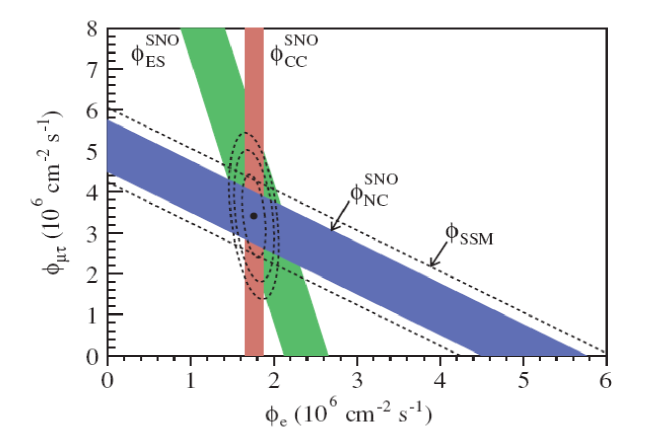
Figure 23: SNO results for the various channels,from reference [86], copyright (2005) by the American Physical Society.

These results are graphically presented in Figure 23.

From the above results we can conclude that

• $R_{ee}=\Phi(CC)/\Phi(NC)=0.34\pm 0.023^{+0.029}_{-0.031}$. 2/3 of $\nu_{e}$ neutrinos have changed their flavor and arrived on earth as $\nu_{\mu}$ and/or $\nu_{\tau}$

• the flux of neutrinos of all flavors (NC flux) is in good agreement with the SSM predictions of (5.05$\pm$0.5)$\times 10^{6}~{}cm^{-2}sec^{-1}$ [87]

Phase 2: 2001-2002 Two tons of NaCl have been added to the heavy water increasing the efficiency of the neutron capture cross section. In the Cl capture process multiple gamma rays are produced, thus neutral current events can be statistically separated from processes 1 and 3, where single electrons are produced. Results for this phase are given in references [88] and [86].

Phase 3: 2003-2006

Neutron detectors have been added, and the analysis is in progress.

The collaboration has decided to stop the experiment at the end of 2006, since the statistical accuracy has reached the systematic one.

A new international laboratory is being constructed, SNOLAB, as an extension of SNO and already a variety of experiments has been proposed [89].

Borexino experiment:

In 2007 the Borexino experiment has published the first result, a direct measurement of Be⁷ solar neutrinos [90]. The low threshold of the experiment, 250 keV, has allowed to measure the Be⁷ flux for the first time in real time. The experiment has been build at the LNGS and detects $\nu_{e}$ via the electron scattering process. The detector is a sphere of 300 tons liquid scintillator (100 ton fiducial mass) viewed by 2200 photomultipliers. The low threshold has been obtained after many years of R$\&$D.

The measurement of neutrinos below 1 MeV allows to study the region between the vacuum and MSW regimes. The best value for the counting rate is

$$47\pm 7_{stat}\pm 12_{syst}~{}counts/100ton/day$$

in good agreement with $49\pm 4$ predicted by the solar model with the solar neutrino oscillation parameters derived from previous experiments (the so called Large Mixing Angle solution). The rate expected with no oscillation is $75\pm 4$ counts/100 ton /day.

The aim of the experiment is to measure the Be⁷ flux at 5$\%$ level.

6.1.3 Summary of solar neutrino experimental results:

The results presented above are summarized in Table 6 from which the following conclusions can be drawn:

reaction	experiment	results	SSM (*)	data/SSM$\approx$	notes
Cl37$\rightarrow$ Ar37	Homestake [2]	2.56$\pm 0.16\pm 0.16$ SNU	7.6${}^{+1.3}_{-1.1}$	0.34
Ga71 $\rightarrow$Ge71	Gallium [44]	67.6 ${}^{+3.7}_{-3.7}$ SNU	128${}^{+9.}_{-7.}$	0.53	(1)
$\nu_{x}+e\rightarrow\nu_{x}+e$	Kamiokande [6]	2.8${}^{+0.19}_{-0.19}$${}^{+0.33}_{-0.33}10^{6}cm^{-2}sec^{-1}$	5.05${}^{+1.}_{.8}$	0.55	(2)
$\nu_{x}+e\rightarrow\nu_{x}+e$	SK [7]	2.35${}^{+0.02.}_{-0.08}10^{6}cm^{-2}sec^{-1}$	5.05${}^{+1.}_{-.8}$	0.47	(2)
$\nu_{x}+e\rightarrow\nu_{x}+e$	SNO [8]	2.39${}^{+0.24}_{-0.23}$${}^{+0.12}_{-0.12}10^{6}cm^{-2}sec^{-1}$	5.05${}^{+1.}_{-.8}$	0.47	(2)
$\nu_{e}+d\rightarrow p+p+e^{-}$	SNO [8]	1.76 ${}^{+.06}_{-.05}$${}^{+0.09}_{-0.09}10^{6}cm^{-2}sec{-1}$	5.05${}^{+1.}_{-.8}$	0.35	(3)
$\nu_{x}+d\rightarrow\nu_{x}+p+n$	SNO [8]	5.09${}^{+.44}_{-.43}$${}^{.46}_{-0.46}10^{6}cm^{-2}sec^{-1}$	5.05${}^{+1.}_{-.8}$	1.	(4)
$\nu_{x}+e\rightarrow\nu_{x}+e$	Borexino [90]	$47^{+7}_{-7}$${}^{+12}_{-12}counts/day/100ton$	75${}^{+4}_{-4}$	0.60	(2)

Table 6: (*) from reference [87], (1) average of the 3 experiments [44], (2) mainly $\nu_{e}$ elastic scattering, (3) $\nu_{e}$ charged current interactions, (4) neutral current process.

• The flux ratio R = measured/SSM predictions is equal to 1 for the NC SNO measurements. This is a convincing proof of the validity of the solar model predictions.

• All experiments that are sensitive mainly to $\nu_{e}$ obtain a ratio R smaller than 1.

• The ratio R depends on the threshold of the experiment i.e. on the flux composition of the observed events. The depression is dependent on the neutrino energy.

6.1.4 Determination of the mixing matrix elements:

For sin$\theta_{13}$=0 electron neutrinos are a mixture of $\nu_{1}$ and $\nu_{2}$ and so the oscillation can be studied in terms of $\Delta m^{2}_{12}$ and $\theta_{12}$. Solar neutrino data identify a unique solution for the above parameters: the Large Mixing Angle solution (LMA) [91]. Solar matter effects largely determine this solution. The matter mixing angle given in Section 3.2 is computed using $\epsilon(x)=2\sqrt{2}G_{F}N_{e}(x)E/\Delta m^{2}_{12}$, where $N_{e}(x)$ is the electron density at position $x$ from the sun center. In the region identified by the LMA solution, accounting for the non constant solar density, the $\nu_{e}$ survival probability can be written as [92]

$$P_{ee}={{1}\over{2}}+{{1}\over{2}}\cos 2\theta_{m12}\cos 2\theta_{12}$$

where $\cos 2\theta_{m12}$ has been computed with the electron density at the center of the Sun.

For pp neutrinos $\cos 2\theta_{m12}\simeq\cos 2\theta_{12}$ and so $P_{ee})=1-{{1}\over{2}}\sin^{2}2\theta_{12}.$

For ⁸B neutrino energies $\epsilon(x)\simeq 1$, $\cos 2\theta_{m12}\simeq-1$ and so $P_{ee}\simeq\sin^{2}2\theta_{12}$.

The SNO results on the flux ratio of CC/NC= $R_{ee}=P_{ee}/1$ then give a direct measurement of $\sin^{2}\theta_{12}$.

Flux differences between day and night (day-night effect), due to MSW effect inside the Earth, are expected to be small for the oscillation parameters of the LMA solution. No evidence for such effect has indeed been found by SK [93] and SNO [86]. Distortions of the energy spectra were also not observed by these experiments, as expected.

Figure 24: Results of combined SNO,SK,CL,Ga results in the parameter plane, from reference  [88], copyright (20042004) by the American Physical Society, the central values for the parameters are $\Delta m^{2}_{12}=6.5\times 10^{-5}$ eV² and tan${}^{2}\theta_{12}=0.4$.

In conclusion the solar results are given in Figure 24.

The correctness of the LMA solution has been confirmed by the KamLAND reactor neutrino experiment, as will be shown in Section 6.2.3.

6.2 Reactor neutrinos

Reactor experiments are designed to detect $\overline{\nu}_{e}$ via the reaction

$$\overline{\nu}_{e}+p\rightarrow e^{+}+n$$

At short distances (see Section 3) the obtained limits can be interpreted in terms of $\theta_{13}$ (CHOOZ results); at large distances the KamLAND experiment results can be interpreted in the two flavor mixing scheme in terms of the 1,2 mixing parameters, the solar ones.

A discussion of main characteristics of experiments with reactor neutrinos is given in [94]. Detectors consist of a tank containing a liquid scintillator surrounded by photomultipliers. The $\overline{\nu}_{e}$ interactions are detected by a coincidence between the prompt signal of the $e^{+}$ and a delayed signal from gamma rays emitted in a capture process of the neutron after its thermalization. The neutron receives negligible kinetic energy so the E($\overline{\nu}_{e}$) is given by the relation

$$T(e^{+})=E(\overline{\nu}_{e})+m(p)-m(n)-m(e)=E(\overline{\nu}_{e})-1.8\mathrm{MeV}$$

where T$(e^{+}$) is the kinetic energy of the positron.

From the above relation we see that the process has a threshold at 1.8 MeV. The number of events collected depends on the mass of detector, on the flux of $\overline{\nu}_{e}$ and on the cross section for the process. Figure 25 shows the anti-neutrino flux (b) cross section (c) and the interaction rate (a) for a 12t detector at 0.8 km from a reactor with thermal power W=12GW.

Figure 25: curves a and b are referred to a 12t fiducial mass detector positioned at 0.8 km from a 12 GW reactor, from reference  [94], copyright (2002) by the American Physical Society.

In the last 20 years many experiments on $\overline{\nu}_{e}$ from reactor have been made [95, 96, 97, 98]. The ratio $L/E$ of these experiments was such that the minimum $\Delta m^{2}$ that could be reached was of the order of $10^{-2}~{}\mathrm{eV}^{2}$.

Two recent experiments CHOOZ [45] and KamLAND [9] have given relevant results in the oscillation field.

Results compatible with the CHOOZ ones have been obtained by the Palo Verde Experiment [99].

6.2.1 CHOOZ experiment:

The experiment was located close to the nuclear power plant of CHOOZ (north of France), a schematic drawing of the detector is shown in Figure 26.

The detector used gadolinium loaded scintillator as neutrino target . Gadolinium has high thermal neutron capture cross section and releases about 8 MeV energy in the process.

The detector was located at about 1 km from the neutrino source in an underground laboratory to reduce the muon flux by about a factor 300 compared to the surface one. Muons produce neutrons by spallation in the material surrounding the detector; these neutrons are one of main sources of background.

Figure 26: The CHOOZ detector, from reference  [94], copyright (2002) by the American Physical Society.

The detector consisted of a central region filled with 5 tons of gadolinium loaded scintillator (0.09$\%$), an intermediate region (107 tons) filled with undoped scintillator to contain the electromagnetic energy produced by the neutron capture in gadolinium and an external region still filled with scintillator, used for muon anti-coincidence.

Data were taken from March 97 to July 98 . The selection criteria for $\overline{\nu}_{e}$ interactions were

• positron energy $\leq$ 8 MeV

• gamma energy released in the neutron capture$\leq$ 12 MeV and $\geq$ 6 MeV

• interaction vertex distance from wall $\geq$ 30 cm

• distance electron-neutron $\leq$ 100 cm

• neutron delay $\leq$ 100 $\mu$sec

• neutron multiplicity =1

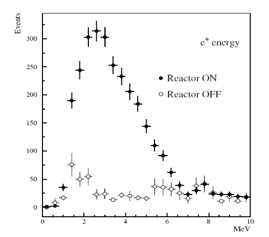
Figure 27: Positron spectra in CHOOZ with reactor ON and OFF, from reference  [45], with kind permission of the European Physical Journal (EPJ).

Figure 27 shows the positron energy spectra with reactor on and reactor off. The positron spectrum after the reactor off spectrum has been subtracted is shown in Figure 8.

The analysis of these data has given, for the ratio of the flux to the unoscillating expectation, the following result

$$R=1.01\pm 2.8\%(stat)\pm 2.7\%(syst).$$

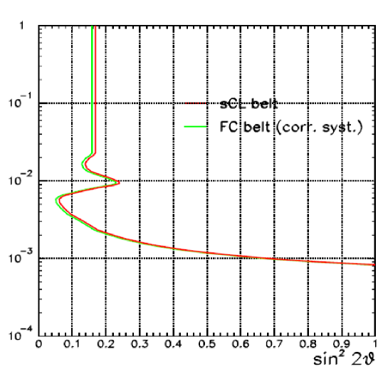
Figure 28: CHOOZ results, from reference  [45], with kind permission of the European Physical Journal (EPJ).

Figure 28 translates this result into limits on the oscillation parameters obtained in the two flavor mixing model. Oscillations $\overline{\nu}_{e}\rightarrow\overline{\nu}_{x}$ are excluded for $\Delta m^{2}\geq 8\times 10^{-4}$ eV². Limits on $\sin^{2}2\theta$ depend on the assumed $\Delta m^{2}$. For the value of $\Delta m^{2}$ given by the atmospheric neutrino the limit $\sin^{2}2\theta\leq 0.13$ is obtained. This limit excludes $\nu_{\mu}\rightarrow\nu_{e}$ oscillations with this $\Delta m^{2}$ value and therefore the possibility of interpreting the SK atmospheric muon neutrino deficit in terms of $\nu_{\mu}\rightarrow\nu_{e}$ oscillations.

6.2.2 Palo Verde experiment:

the Palo Verde experiment was built at the Palo Verde Nuclear Generating Station in Arizona. There were 3 identical reactors with a thermal power of 11.6 GW. The detector consisted in 66 acrylic tanks filled with gadolinium loaded scintillator, with a total mass of 11 ton. The experiment did run from 1998 to 2000. The final result expressed as the ratio R, observed rate over expected one with no oscillation, was [99]:

$$R=1.01\pm 2.4\%(stat)\pm 5.3\%(syst).$$

6.2.3 KamLAND experiment:

KamLAND is situated under 2700 MWE in the Kamioka (Japan) mine laboratory in the old site of the Kamiokande experiment. Data reported here have been taken between March 2002 and January 2004.

53 power reactors surround KamLAND at an average distance of 150 km. The detector consists of 1 kton pure scintillator contained in a 13 m diameter balloon suspended in non scintillating oil. The balloon is viewed by 1879 photomultipliers (Figure 29).

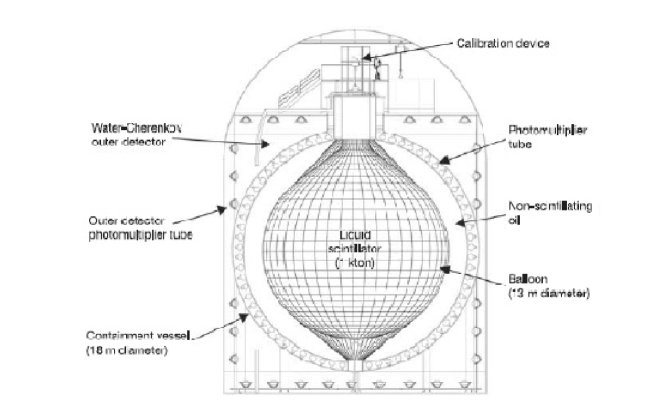
Figure 29: The KamLAND detector, from reference  [100], copyright (2003) by the American Physical Society.

Neutrons are detected by the capture of neutron on proton (capture energy=2.2 MeV). The selection criteria were

• fiducial volume with radius $\leq$ 5 m

• gamma energy released in the neutron capture $\leq$ 2.6 MeV and $\geq$ 1.8 MeV

• distance from wall $\geq$ 30 cm

• distance electron-neutron $\leq$ 160 cm

• neutron delay $\leq$ 660 $\mu$sec

• neutron multiplicity =1

The main sources of background are neutrons from spallation produced by fast muons and delayed neutrons emitted by He⁸ and Li⁷. The expected non oscillation number of events above 2.6 MeV was 365 $\pm$ 23 (syst). The number of observed events was 258, with an expected background of 17.8 $\pm$ 7.3 events. The survival probability has been estimated to be

$$0.658\pm.044stat\pm 0.047syst.$$

The total spectrum is shown in Figure 30left. Above 2.6 MeV one can see data and expected spectrum without oscillation. Below 2.6 MeV, subtracting background, one can estimate 25 $\pm$ 19 events that could be indication of geological neutrinos. Geological neutrinos are generated by the decay of radioactive elements (uranium, thorium and potassium) inside the earth, they are of geological interest. Figure 30right gives the $L/E$ distribution of events above 2.6 MeV. The blue line gives the best fit result for oscillation. Alternative models, neutrino decay [101] and decoherence  [102], are ruled out. These data therefore support the interpretation of the effect as due to neutrino oscillation. The neutrino spectrum modulation of the KamLAND Experiment allows a measurement of $\Delta m^{2}_{12}$ more precise than the one obtained by solar neutrino experiment.

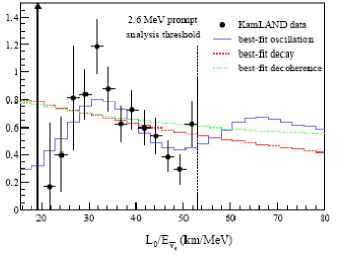
Figure 30: left: Energy distribution; right: L/E distribution for anti-neutrinos, from reference [9], copyright (2005) by the American Physical Society.

A global two flavor analysis of KamLAND data and solar data [9] gives

$$\Delta m^{2}=(7.9^{+0.6}_{-0.5})\times 10^{-5}~{}\mathrm{eV}^{2}$$

$$\tan^{2}\theta=0.40^{+0.10}_{-0.07}.$$

Figure 31 presents the final result of the KamLAND+Solar parameters determination a) KamLAND+Solar results, b) combined fit.

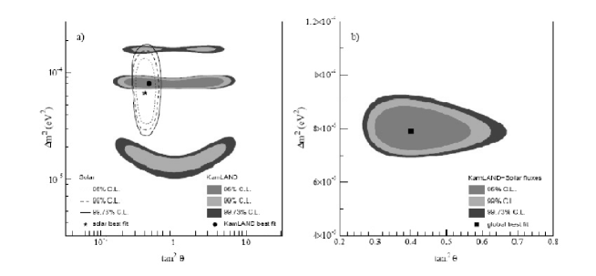
Figure 31: Accepted values for oscillation parameters KamLAND +Solar a) dashed region KamLAND allowed region and solar neutrino experiments (lines) b) combined results from reference [9], copyright (2005) by the American Physical Society.

A complete discussion of the oscillation parameters will be made in section 7.

After the KamLAND result the LMA solution is well established and the oscillation parameters 1,2 are determined with a good accuracy.

Future experiments will be mainly devoted to obtain more information on solar model and checks of the LMA solution for oscillations.

KamLAND has started a second phase of the experiment in which elastic scattering of solar neutrinos will be detected with the same aim of Borexino. The background level will be reduced at least a factor 100 compared to the present one. If the goal of background rejection will be reached the expected rate from Be⁷ in the energy window 280-800 KeV will be much larger than in Borexino (1000 ton against the 100 ton of Borexino).

Proposals for pilot experiments and R$\&$D for a series of future experiments aiming at the detection of pp, CNO and Be⁷ neutrinos have been presented [103].

6.3 Atmospheric neutrinos:

Atmospheric neutrinos must be observed in underground detectors because of the background due to cosmic rays.

For low energy neutrinos the observation of the neutrino interactions with fully contained reaction products is possible with reasonable efficiency (fully contained events, FC).

When the energy increases, the muon produced in $\nu_{\mu}$ CC interactions has a high probability to escape the detector (partially contained events, PC).

There is a third category of $\nu_{\mu}$CC events: upward going muons produced in the rock. They can stop (stopping muons) or traverse the detector (through-going muons). Cosmic rays muons cannot be distiguished from the neutrino produced ones so this technique cannot be used for muons coming from top. The typical energy is of the order of 10 GeV for stopping muons and 100 GeV for traversing ones. The neutrino energy will be larger than the observed muon one.

To study the neutrino interaction Monte Carlo programs have been developed [48, 50, 51, 49, 47, 46] to predict the ratio $\nu_{e}$/$\nu_{\mu}$ to be compared with the experimental observations. The double ratio,

$$\frac{(\nu_{\mu}/\nu_{e})_{data}}{(\nu_{\mu}/\nu_{e})_{MC}}$$

expected to be 1 in absence of oscillations, has been determined by several experiments and has always been found to be smaller than 1 [13, 104, 105, 106].

The rate of up going muons can be compared with the MC predictions and also here the rates are smaller than expectations [12, 82]. The amount of the effect depends on the used Monte Carlo generator more than the double ratio.

The final confirmation of the interpretation of the deficit as due to $\nu_{\mu}$ neutrino oscillation came in 1998 [11] when Super-Kamiokande demonstrated a clear difference between upward and downward muon neutrinos, while no difference was seen in the electron neutrino.

The upward neutrinos traverse the Earth (12000 km), the downward come from the atmosphere (20 km). We shall discuss in the following some of the cited experiments.

6.3.1 The Kamiokande and Super-Kamiokande experiments:

The Kamiokande and Super-Kamiokande detectors already discussed in the solar neutrino section have been used in the detection of atmospheric neutrinos. Now the energy range (see Figure 9) of studied events is of the order of GeV, so $\nu_{\mu}$ can be detected via their CC reactions. The flavor of $\nu$ is determined through the observation of the shape of Cherenkov light emitted by the lepton produced in the final state.

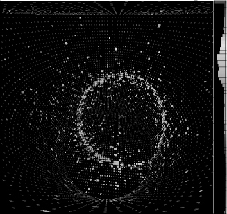
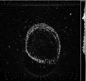
Figure 32: Examples of an electron and a muon ring in SK detector, from http://www.ps.uci.edu/$\sim$tomba/sk/tscan/pictures.html

Muons originate a ring with well defined borders while electrons have blurred contours (Figure 32).

Super-Kamiokande [11] demonstrated a clear difference between upward and downward going muon neutrinos compared with the MC predictions, while no difference was seen for electron neutrinos.

In the analysis atmospheric neutrino data were subdivided in

• Fully contained (FC) events Sub-GeV Evis $\leq$ 1.33 GeV

• Fully contained events Multi-GeV Evis $\geq$ 1.33 GeV

  FC events were divided in single ring or multiple ring. Single ring were classified as e-like or $\mu$-like according to the characteristic of the Cherenkov cone. Multiring were classified as e-like or $\mu$like according to the characteristic of the highest energy cone.

• Upward going muons.

  Muons traveling up were divided in muons stopping in the detector (stopping muons) or traversing (through-going muons).

The results of Super-Kamiokande, Soudan-2 and MACRO are shown in Figure 33 [107].

Figure 33(top) from reference [107] shows the angular distribution for the SK events categories defined above.

We see that for electrons the distributions are well represented by the MC while for muons events coming from bottom, negative cos$\theta$ events are missing.

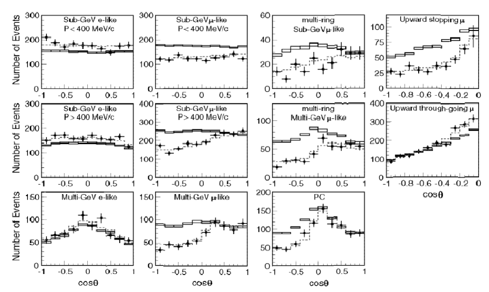
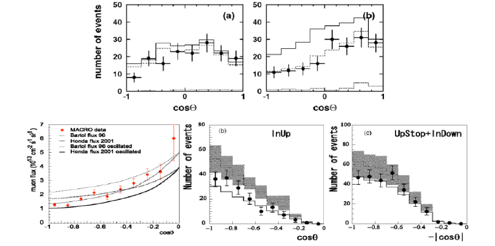
Figure 33: Angular distributions of atmospheric events, from reference  [107], copyright (2005), with permission from Elsevier.

Figure 33(middle) shows the angular distribution for the Soudan-2 experiment, we still see missing events in the muon distribution (b).

Figure 33 bottom shows the angular distribution of upgoing muons in MACRO.

The SK Collaboration [106], for the ratio $(\mu/e)_{data}/(\mu/e)_{MC}$ that should be 1 in the absence of oscillations, quotes for Sub-GeV events

$$R=0.658\pm 0.016\pm 0.035$$

and for for Multi-GeV+PC

$$R=0.702\pm 0.03\pm.101$$

a two flavor oscillation analysis has been been made [106] with results

$$\sin^{2}2\theta\geq 0.92(90\%CL)$$

$$1.5\times 10^{-3}\leq\Delta m^{2}\leq 3.4\times 10^{-3}\mathrm{eV}^{2}$$

(see Figure 34).

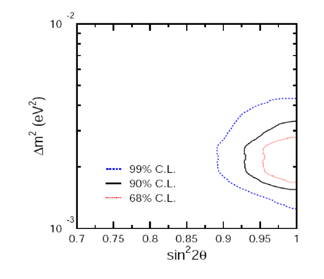
Figure 34: SK atmospheric fit results, from reference  [106], copyright (2005) by the American Physical Society.

Analysis in the three flavor mixing scheme is discussed in [108].

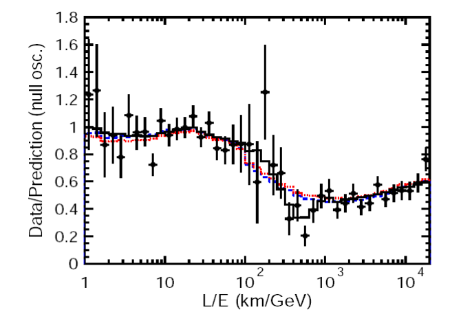
Figure 35: Ratio of data to MC events without neutrino oscillation (points) as a function of the reconstructed L/E together with the best-fit expectation for two flavor $\nu_{\mu}\rightarrow\nu_{\tau}$ oscillations(solid line) [109], copyright (2004) by the American Physical Society. Also shown are the best-fit expectation for neutrino decay (dashed line) and neutrino decoherence (dotted line).

Selecting well measured events a plot of L/E has been obtained and is shown in Figure 35 [109]. The presence of a dip in the L/E distribution gives strong support to the oscillation interpretation against other possible explanations. Figure 35 in fact shows that alternative explanations do not reproduce the dip.

Figure 36 shows the results of the zenith angle analysis and of the L/E one. The position of the dip allows a better determination of the $\Delta m^{2}$ region in the L/E analysis compared with the one obtained from analysis of the zenith angle.

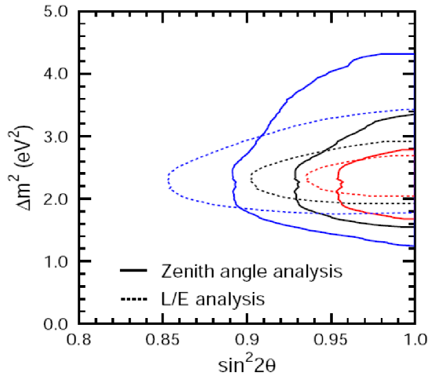
Figure 36: The 68, 90 and 99 $\%$ confidence level allowed oscillation parameter regions obtained by the SK L/E and zenith angle analysis, from reference  [106], copyright (2005) by the American Physical Society.

We will now briefly describe the other experiment that did confirm the SuperKamiokande results.

6.3.2 The MACRO experiment:

the MACRO Experiment [12] located in the Gran Sasso Laboratory (LNGS) took data from 1995 to 2000. It did consist of three independent detectors: liquid scintillators counters, limited streamer tubes and nuclear track detectors (not used in the oscillation search). The detector did reveal upgoing muons coming from interactions in the rock. In the analysis the angular distribution and the absolute flux compared with the Monte Carlo predictions were used, see Figure 33(bottom). The analysis in terms of oscillation did favour maximum mixing and $\Delta m^{2}=0.0025~{}eV^{2}$.

6.3.3 The Soudan-2 experiment:

Soudan-2 [13] was a 770 ton fiducial mass detector that did operate as a time projection chamber. The active elements of the experiments were plastic drift tubes. The detector was located in Minnesota (USA). The experiment did run from 1989 to 2001 with a total exposure of 5.90 kton-years. An analysis in terms of oscillation parameters of the L/E distribution gave as result $\Delta m^{2}=0.0025~{}eV^{2}$ and $sin^{2}2(\theta)=0.97$.

6.3.4 The MINOS experiment:

The far detector of the MINOS experiment [62], described in Section 6.4.3, is designed to study neutrinos coming from the neutrino beam NuMI at the Fermilab National Laboratory. The experiment can also detect atmospheric neutrinos and being a magnetized detector it has the advantage to observe separately $\nu$ and $\overline{\nu}$ measuring the charge of muons in the magnetic field.

The data relative to a period of 18 months (2003-2005) are consistent with the same oscillation parameters for neutrinos and anti-neutrinos. In fact MINOS quotes [110]

$$\frac{(\overline{\nu}_{\mu}/\nu_{\mu})_{expt}}{(\overline{\nu}_{\mu}/\nu_{\mu})_{mc}}~{}~{}=.96^{+0.38}_{-0.27}(stat)\pm 0.15(syst)$$

and

$$\frac{(up/down)_{exp}}{(up/down)_{mc}}~{}~{}=.62^{+0.19}_{-0.14}(stat)\pm.02(syst)$$

that still gives an indication of upward going muon disappearance. These results are statistically limited and correspond to a statistics of 4.54 kiloton-year. From their analysis the hypothesis of no oscillation is excluded at the $98\%$ of CL.

6.4 Accelerator neutrinos:

Neutrino beams (see Section 4.4) have been produced in accelerators since the 60’s. The possibility of doing neutrino experiments at accelerators was first proposed by B. Pontecorvo in 1957 [111] and M. Schwartz in 1960 [112]. Following these suggestions an experiment was performed at the Brookhaven National Laboratory in which the muon neutrino was discovered [113]. For what concerns oscillation experiments we can divide them in two categories, short baseline (see Section 6.4.1) and long baseline (see Section 6.4.3). The range of the $\Delta m^{2}$ that have been detected has pushed toward the second type experiments.

6.4.1 Short baseline experiments:

Search for $\nu_{\mu}\rightarrow\nu_{e}$

.

A) Bubble chamber experiments

Bubble chambers experiments did begin in the ’70s. These experiments that gave important results in neutrino physics could provide only limits in the oscillation parameters space.

Experiments were made in CERN Gargamelle [114], CERN BEBC (the Hydrogen bubble chamber)[115] and in the Fermilab 15 ft bubble chamber [116]. The last experiment with bubble chambers in CERN was the BEBC experiment with a low energy neutrino beam to search for $\nu_{\mu}\rightarrow\nu_{e}$ for values of $\Delta m^{2}\approx$ 1 eV² [61].

Experiment	Beam Mean Energy	$\Delta m^{2}$ (eV2)	$\sin^{2}2\theta\times 10^{-3}$
	(Gev)	$(\sin^{2}2\theta=1)$	(large $\Delta m^{2}$)
Gargamelle CERN [114]	300	1.2	10.
BEBC CERN [115]	300	1.7	10.
15 foot BC Fermilab [116]	30	0.6	6.
BEBC CERN [61]	1.5	0.09	13.

Table 7: $\nu_{\mu}-\nu_{e}$ limits in bubble chamber experiments .

B) Electronic detectors experiments

Electronic detectors searches were made using general purpose neutrino detectors [53, 54, 55, 117, 118, 119] or dedicated detectors[57, 56].

Several experiments were made to search for $\nu_{\mu}\rightarrow\nu_{e}$ with electronic detectors. A non exhaustive list is given in Table 8.

Experiment	Neutrino Mean Energy	$\Delta m^{2}$ (eV2)	$\sin^{2}2\theta\times 10^{-3}$
	(GeV)	$(\sin^{2}2\theta=1)$	(large $\Delta m^{2}$)
CHARM CERN [120]	25.	0.19	8
E776 BNL [121]	5.	0.075	3
E734 BNL [122]	5.	0.03	3.6
CHARM2 CERN [123]	25.	8.5	5.6
NUTEV FNAL [124]	140.	2.6	1.1
NOMAD CERN [125]	25.	0.4	1.4

Table 8: $\nu_{\mu}-\nu_{e}$ limits in accelerator experiments.

All these experiments were made with conventional neutrino beams and gave negative results. The $\nu_{e}$ were detected through their charged current interactions giving an electron. The $\nu_{e}$ contamination of the beam that had to be subtracted was one of the main sources of systematic errors. The other systematic error was the contamination of gamma rays from $\pi^{0}$ decay.

Search for $\nu_{\mu}\rightarrow\nu_{x}$

.

Experiments were also made on disappearance of $\nu_{\mu}$, $\nu_{\mu}\rightarrow\nu_{x}$. Muons from CC $\nu_{\mu}$ interactions were counted. In this case two detector systems at different distances were used to eliminate the uncertainties on the knowledge of neutrino fluxes. For two detectors experiments the excluded region closes up at high $\Delta m^{2}$ when oscillation happens in both detectors. Results are summarized in Table 9.

Experiment	Neutrino Mean Energy(GeV)	$\Delta m^{2}$ min eV2	$\Delta m^{2}$ max eV2
CDHS CERN [59]	25.	0.23	100.
CHARM CERN [60]	25.	0.29	22.6
FNAL [116]	140.	8.	1250

Table 9: Limits on the disappearance for $\nu_{\mu}-\nu_{x}$

Search for $\nu_{\mu}\rightarrow\nu_{\tau}$

.

The detection in appearance mode of $\nu_{\mu}\rightarrow\nu_{\tau}$ is difficult because of the short lifetime of the $\tau$ whose flight length is $\leq$ 1mm. Following a negative result from the emulsion experiment E531 at Fermilab[126], there have been two experiments at the CERN WBB searching for small mixing angles and relatively large $\Delta m^{2}$. In these experiments the E/L ratio of the beam is indeed large because the energy has been set to have an appreciable $\nu_{\tau}$ cross section.

The CHORUS experiment [56] was a hybrid emulsion electronic detector that had excellent space resolution at the $\tau$ decay.

The NOMAD [57] experiment, where the vertex resolution was not good enough to see the tau decay, applied kinematical criteria to search for $\nu_{\tau}$CC. Both experiments gave a negative result as shown in Table 10.

Experiment	Neutrino beam energy (GeV)	$\Delta m^{2}$ eV${}^{2}~{}(\sin^{2}2\theta=1)$	$\sin^{2}2\theta(large\Delta m^{2})$
NOMAD CERN [39]	25.	0.7	3$\times 10^{-4}$
CHORUS CERN [38]	25.	0.6	4.4$\times 10^{-4}$

Table 10: $\nu_{\mu}-\nu_{\tau}$ limits.

6.4.2 Other short baseline experiments:

LSND, KARMEN and MiniBooNE.

There is one experiment that has claimed to have seen oscillations in the region $\Delta m^{2}\leq 1$ eV², the LSND [65] experiment.

The experiment was run in 1993-1998 at the LAMPF accelerator in Los Alamos (USA). The detector consisted of a tank containing 168 ton of liquid scintillator equipped on the inside surface with 1220 photomultipliers.

The intense proton beam ($\simeq$  1mA), at an energy of 798 MeV, produces a large number of pions mostly $\pi^{+}$ that then decay in $\mu^{+}+\nu_{\mu}$. The $\mu^{+}$ decays at rest in $e^{+}+\nu_{e}+\overline{\nu}_{\mu}$. Practically all $\pi^{-}$ are absorbed in the shielding. The $\overline{\nu}_{e}$ flux coming from the $\mu^{-}$ decay at rest, where $\mu^{-}$ are produced in the rare $\pi^{-}$ decay in flight, constitutes a small fraction of the $\overline{\nu}_{\mu}$ one. Consequently the experiment, through the study of the process $\overline{\nu}_{e}+p\rightarrow e^{+}+n$, allows the study of the $\overline{\nu}_{\mu}\rightarrow\overline{\nu}_{e}$ oscillation.

The study of the process $\nu_{e}+C~{}\rightarrow e^{-}+N$, using only electrons above the Michel endpoint to eliminate the $\nu_{e}$ from $\mu^{+}$ decay, did allow the study of the process $\nu_{\mu}~{}\rightarrow~{}\nu_{e}$. LSND found an excess of e⁺ (e^-) [65] and made a claim for oscillations with parameters $\Delta m^{2}=1.2$ eV², $\sin^{2}2\theta=0.003$, as shown in Figure 37.

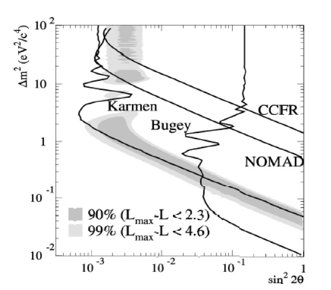
Figure 37: LSND results ,($\sin^{2}2\theta,\Delta m^{2}$oscillation parameters fit), the inner and outer regions correspond to 90$\%$ and 99$\%$ allowed, from reference  [65], copyright (2001) by the American Physical Society.

A similar experiment, KARMEN [127], ran at the ISIS pulsed spallation neutron source in UK in 1997 and 1998 and did not give any positive evidence. It covered a large fraction of the LSND results, as shown in Figure 37. New experiments were needed. The MiniBooNE experiment, designed at Fermilab, is now running. The experiment uses the Fermilab booster (8 GeV protons) neutrino beam. The detector is a spherical tank of inner radius of 610 cm filled with 800 tons of mineral oil. The Cherenkov and scintillation light is collected by photomultipliers.

The first publication of the experiment does not confirm the LSND results [128] (see Figure 38).

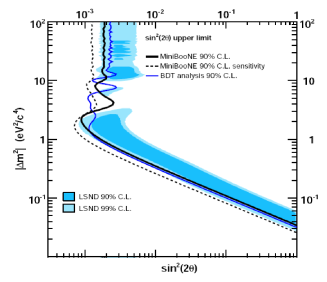
Figure 38: MiniBooNE 90$\%$ confidence level, shaded area corresponds to LSND result ,from reference [128], copyright (2007) by the American Physical Society.

Had the LSND claim been confirmed, then a major change in the theory would have been needed. With only 3 neutrinos there are two independent $\Delta m^{2}$ values, that we identify with the solar and atmospheric ones. The LSND result, introducing a third $\Delta m^{2}$ value, would have required a fourth, unobserved, sterile neutrino.

6.4.3 Long baseline accelerator experiments:

Man-made neutrino sources experiments are very important in providing the final confirmation of neutrino oscillations. The solar result confirmation was given by KamLAND. To confirm the atmospheric ones, dedicated long baseline neutrino experiments have been conceived, providing access to the same L/E range. The K2K experiment has been completed and first results from MINOS have been given, while OPERA starts to take data. The three experiments are described below.

The K2K experiment:

The experiment [14] used an accelerator produced $\nu_{\mu}$ neutrino beam of an average energy of 1 GeV, the neutrino interactions were measured in the SK detector located at 250 km from the source and in a close detector located at 300 m from the target. A total of 10²⁰ protons have been delivered to the target in the data taking period 1999-2001. The SK detector has already been presented in Section 6.1.2. The close detector consists of 1 kiloton water Cherenkov detector and a scintillating fiber water target (SCIFI). In the second data taking period (K2K II) a segmented scintillator tracker (SCIBAR) and a muon ranger (MRD) were added to it. The experiment is a disappearance experiment since the energy of the beam is below the threshold for $\nu_{\tau}$ production. The oscillations are detected by the measurement of the flux ratio in the two detectors and by the modulation of the energy distribution of CC produced events. The energy distribution of events can be obtained from the SK 1-ring events that are assumed to be quasi elastic (at the K2K energies 1 ring mu events have a high probability to be quasi elastic). In this approximation

$$E_{\nu}^{rec}=(M_{n}E_{\mu}-m_{\mu}^{2}/2)/(M_{n}-E_{\mu}+P_{\mu}\cos\theta_{\mu}).$$

The expected number of events in SK in the absence of oscillation is 158, the measured one is 122. The expected number has been obtained from the rate of events measured in the close detector. The comparison between the SK spectrum and the expected one in absence of oscillation is shown in Figure 39.

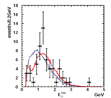
Figure 39: K2K $E_{\nu}$ distribution for 1 ring $\mu$ events. Points with error bars represent data, solid line the best fit with oscillations while the dashed line shows expectation without oscillations, from reference [14], copyright (2006) by the American Physical Society.

The best fit results [14] obtained combining the information from the spectrum shape and the normalization are

$$\sin^{2}2\theta=1~{}~{}~{}~{}\Delta m^{2}=2.8\times 10^{-3}\mathrm{eV}^{2}~{}(1.8\times 10^{-3}\leq\Delta m^{2}\leq 3.5\times 10^{-3}~{}\mathrm{at}~{}90\%~{}~{}CL)$$

the probability of no oscillation hypothesis is 0.0015$\%~{}(4.3~{}\sigma)$.

Figure 40 shows K2K results compared to Super-Kamiokande results obtained with atmospheric neutrinos.

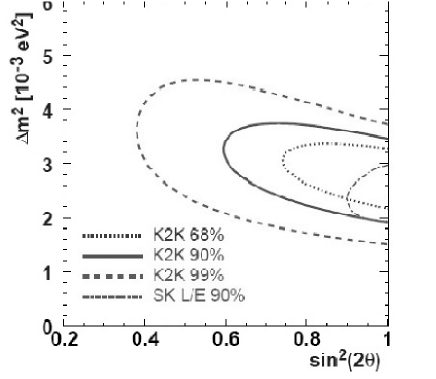
Figure 40: Comparison of the K2K results with the SK atmospheric neutrino in the parameter space, dotted, solid, dashed and dashed-dot represent the 68, 90, 99 $\%$ CL allowed regions of K2K and 90 $\%$ CL for SK atmospheric, from reference  [14], copyright (2006) by the American Physical Society.

A search for $\nu_{\mu}\rightarrow\nu_{e}$ has been also performed [129] and the result for $\Delta m^{2}=2.8\times 10^{-3}\mathrm{eV}^{2}$ is $\sin^{2}2\theta_{\mu e}$ $<$ 0.13 at 90 $\%$ CL. This limit will be discussed in Section 7. together with all the results on $\sin^{2}2\theta_{13}$.

The MINOS experiment:

The MINOS experiment [62] is a $\nu_{\mu}$ disappearance experiment using two detectors, the Near Detector (ND) and the Far Detector (FD).

The ND detector (0.98 kton) is located at 103 m underground and at a distance of 1 km from the source. The FD detector, 705 m underground, is located at a distance of 735 km. The detectors are magnetized iron calorimeters made of steel plates of 2.54 cm thickness interleaved with plastic scintillator planes segmented into strips (4.1 cm wide and 1 cm thick).

Data have been collected in the period May 2005-February 2006 and a total of 1.27$\times 10^{20}$ protons were used in the target position that gives the “LE Beam” (see Figure 14) the one that maximizes the neutrino flux at low energies [37].

215 events with an energy $\leq$ 30 GeV have been collected in the FD to be compared with an expected number of 336 $\pm$ 14.

The observed reconstructed number of events is compared (bin by bin) in Figure 41

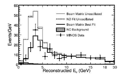
Figure 41: MINOS comparison of the $E_{\nu}$ spectra with oscillations with the no oscillations one, from reference [130], copyright (2006) by the American Physical Society.

to the expected number of events for the oscillation hypothesis. The results are

$$\Delta m^{2}_{23}=2.74^{+0.44}_{-0.26}\times 10^{-3}~{}\mathrm{eV}^{2}$$

and $\sin^{2}2\theta_{23}\geq 0.87~{}at~{}68\%~{}CL$ [37] (figure 42).

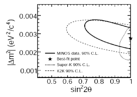
Figure 42: MINOS confidence limits for the oscillations parameters, from reference [37].

Preliminary results with increased statistics (2.5$\times 10^{20}$) protons have been presented at the TAUP2007 Conference; the updated value for $\Delta m^{2}_{23}$ is $2.38^{+0.20}_{-0.16}\times 10^{-3}$ eV² [131].

The OPERA experiment:

The overall neutrino oscillation picture is still lacking the direct observation of a different flavor in a neutrino $\nu_{\mu}$ beam. This is the aim of the OPERA [132] experiment that is designed to detect $\nu_{\tau}$ appearance in a $\nu_{\mu}$ beam. The high mass of the $\tau$ lepton requires a high energy neutrino beam. The CNGS (CERN to Laboratori Nazionali del Gran Sasso) neutrino beam has been optimized to study these oscillations. The average energy at LNGS is 17 GeV, the contamination of $\nu_{e}$ or $\overline{\nu}_{e}$ is smaller than 1 $\%$ and the $\nu_{\tau}$ one is completely negligible.

The detector is made of two identical super modules, each one consisting of a target section of 900 ton lead/emulsion modules (using the Emulsion Cloud chamber technique illustrated in Figure 43), of a scintillator tracker detector and of a muon spectrometer. The high spatial resolution (1 micron) of the emulsions allows the detection of the $\tau$ flight path before its decay. Decay lengths are of the order of 1 mm.

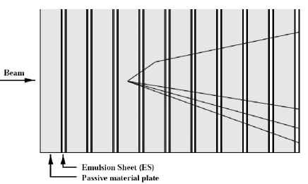
Figure 43: ECC structure in OPERA, from reference [132]

In 5 years of run, with $4.5\times 10^{19}$ p.o.t./year, 30k neutrino interactions will be detected. Assuming a $\Delta m^{2}_{23}$ of $2.5\times 10^{-3}$ eV² the number of tau detected will be order of 10 with a background of about 1. It must be noted that at large $\sin^{2}2\theta$ and $\Delta m^{2}\ll L/E$ the number of produced events depends quadratically from $\Delta m^{2}$, so the number of detected events will be 14 at $\Delta m^{2}=3\times 10^{-3}$ eV² and 6 at $\Delta m^{2}=2\times 10^{-3}$ eV².

The experiment will also be able to give limits on $\nu_{\mu}\rightarrow\nu_{e}$. A limit of 0.06 on $\sin^{2}2\theta_{13}$ can be reached with $\sin^{2}2\theta_{23}$=1 and $\Delta m^{2}_{23}=2.5\times 10^{-3}$ eV² [133].

The beam and the detector performances (no emulsion inserted) have been successfully tested in August 2006 [134]. Reconstruction of neutrino events in the EEC has been accomplished in 2007. Details on the reconstruction of these events is given in reference [135].

7 Present knowledge of the parameters of the mixing matrix

Flavor and mass eigenstates are connected by the unitary matrix U that in the general case of (3,3) mixing is defined by 3 angles and possibly a phase factor $\delta$ (see Section 3.1.1). With 3 neutrino species there are two independent mass square differences.

While the present experiments cannot access $\delta$, we will now summarize our present knowledge of the above parameters. The small value of $\alpha=\Delta m^{2}_{solar}/\Delta m^{2}_{atmospheric}$ and the smallness of $\sin^{2}\theta_{13}$ allows in first approximation the two flavors treatment of neutrino oscillations for atmospheric and solar neutrinos.

$\Delta m^{2}_{23}$ and $\sin^{2}(2\theta_{23})$

The atmospheric experiments, K2K and MINOS, measure essentially the $\nu_{\mu}$ survival probability, which in the limit of $\sin\theta_{13}\simeq 0$ and $\sin^{2}(\Delta m^{2}_{12}L/4E)\ll 10$, can be expressed as (see Section 3.1.2)

$$P(\nu_{\mu}\rightarrow\nu_{\mu})=1-\sin^{2}(2\theta_{23})\sin^{2}(\Delta m^{2}_{23}L/4E)$$

identifying $\theta_{23}$ and $\Delta m^{2}_{23}$ with $\theta_{atm}$ and $\Delta m^{2}_{atm}$ and with K2K and MINOS parameters.

The more recent results for these parameters are given in Table 11.

experiment	$\Delta m^{2}\cdot 10^{-3}~{}\mathrm{eV}^{2}$	$\sin^{2}2\theta$
ATMO SK [106]	1.5-3.4	$\geq$ 0.92
K2K [14]	1.5-3.9	$\geq$ 0.58
MINOS [37]	2.48-3.18	$\geq$ 0.87

Table 11: limits on the 23 mixing parameters

$\Delta m^{2}_{12}$ and $\sin^{2}(2\theta_{12})$

The $\nu_{e}$ solar experiments are sensitive mainly to these two quantities (only to these in the two flavor mixing scheme). The long distance reactor experiment KamLAND on $\overline{\nu}_{e}$ is also sensitive (Section 3.1.2) to $\sin^{2}(2\theta_{12})$ and $\Delta m^{2}_{12}$. In this experiment the shape of the energy distribution allows a precise determination of $\Delta m^{2}_{12}$ while the solar experiments have a better sensitivity to $\theta_{12}$. A combined analysis using these informations (and assuming CPT invariance) has given the following results [9]

$$\Delta m^{2}_{12}~{}~{}=7.9^{+0.6}_{-0.5}\times 10^{-5}~{}\mathrm{eV}^{2}$$

$$\tan^{2}\theta_{12}=0.40^{+0.10}_{-0.07}$$

$\sin^{2}(2\theta_{13})$

Short distance reactor experiments are sensitive to $\sin^{2}(2\theta_{13})$ (see Section 6.2). The following limits (90$\%$ CL) were obtained:

$$CHOOZ~{}\cite[cite]{[\@@bibref{}{apollonio}{}{}]}\sin^{2}(2\theta_{13})\leq 0.13$$

$$PaloVerde~{}\cite[cite]{[\@@bibref{}{palo}{}{}]}\sin^{2}(2\theta_{13})\leq 0.17$$

In the three flavor mixing scheme with one $\Delta m^{2}$ dominance we have in $\nu_{\mu}\rightarrow\nu_{e}$ experiments for $\sin^{2}\theta_{23}=0.5$

$$\sin^{2}2\theta_{\mu e}=\sin^{2}2\theta_{13}\sin^{2}\theta_{23}={{1}\over{2}}\sin^{2}2\theta_{13}$$

K2K limit is $\sin^{2}(2\theta_{13})\leq 0.26$ [129], while SK on atmospheric neutrinos gives $\sin^{2}(\theta_{13})\leq 0.14$ [108].

Global fits

Several global fits to neutrino oscillations have been published (Maltoni [136], Fogli [92], Schwetz [137]).

We give as examples

A) The Fogli results

$$\sin^{2}\theta_{13}~{}=0.9^{+2.3}_{-0.9}\times 10^{-2}$$

$$\Delta m^{2}_{12}~{}~{}=7.92^{+0.09}_{-0.09}\times 10^{-5}~{}\mathrm{eV}^{2}$$

$$\sin^{2}\theta_{12}~{}=0.314^{+0.18}_{-0.15}$$

$$\Delta m^{2}_{23}~{}~{}=2.4^{+0.21}_{-0.26}\times 10^{-3}~{}\mathrm{eV}^{2}$$

$$\sin^{2}\theta_{23}~{}=0.44^{+0.41}_{-0.22}$$

B) The Schwetz results

($\sin^{2}\theta_{13}$  not fitted  and assumed to be $\leq~{}~{}0.025~{}~{}$ at 2$\sigma~{}~{}level$)

$$\Delta m^{2}_{12}~{}~{}=7.9^{+0.3}_{-0.3}\times 10^{-5}~{}\mathrm{eV}^{2}$$

$$\sin^{2}\theta_{12}~{}=0.30^{+0.02}_{-0.07}$$

$$\Delta m^{2}_{23}~{}~{}=2.5^{+0.20}_{-0.25}\times 10^{-3}~{}\mathrm{eV}^{2}$$

$$\sin^{2}\theta_{23}~{}=0.50^{+0.08}_{-0.07}$$

These two fits have been made using all the available information and provide compatible results, also in good agreement with the independent two flavor analysis.

The present situation is that we have two values of $\Delta m^{2}$ but what is still not measured is the sign of $\Delta m^{2}_{23}$ (i.e. mass hierarchy). In the current data there is not enough information to determine the phase of the mixing matrix. In conclusion the missing measurements are

• $\sin^{2}\theta_{13}$

• mass hierarchy

• phase $\delta$

To these points will be dedicated the new experiments that will be described in next two sections.

8 Next generation of oscillation experiments

A relatively large value of $\theta_{13}$ above $10^{-3}$ would open the possibility of studying of CP violation in the leptonic sector. Therefore future experiments will be mainly devoted to the measurements of the $\theta_{13}$ parameter. There are two possibilities for measuring $\theta_{13}$: accelerator and reactor experiments. Accelerator $\nu_{\mu}\rightarrow\nu_{e}$ appearance experiments allow the measurement of the three oscillation parameters (sign of $\Delta m^{2}$, $\theta_{13}$, $\delta$). This apparent advantage introduces ambiguities in the interpretation of the results and correlations between the measured parameters. Reactor experiments, being disappearance experiments, cannot display CP or T violations [138] and therefore determine directly the angle $\theta_{13}$.

8.1 Reactor experiments

Several experiments have been proposed, some of them are already approved (at least at a level of R&D) by funding agencies. Table  12, based on the presentation of K.Heeger in TAUP2007 conference [103], summarizes these projects.

location	power	dist Near/Far	depth	target mass	limit	time
	(GW)	(m)	(MWE)	(kton)	(10-2)	(year *)
ANGRA (1) [139], Brasil	4.6	300/1500	250/2000	500	0.5.
DAYA BAY (2),China [140]	11.6	360(500)/1750	260/910	40	1.	3
Double CHOOZ (3) ,Fr [141]	6.7	1050/1067	60/300	10.2	3.	5
KASKA (4), Japan [142]	24.	350/1600	90/260	6.	2
RENO (5) Korea [143]	17.3	150/1500	230/675	20	2	3

Table 12: proposed reactor $\theta_{13}$ neutrino Experiments, (*) time needed to reach limit in years after completition of construction. (1) Angra proposed and R$\&$D, (2) DAYABAY construction starts in 2007, (3) Double CHOOZ construction under way, (4) Proposal, (5)Proposal

Main points to increase the sensitivity of future experiments will be

• higher reactor power, for the reduction of statistical errors

• at least two detectors configuration, for the reduction of reactor systematic errors

• sufficient over burden and active shielding for reduction of background

• improved calibrations and monitoring

Within the approved experiments the best sensitivity is claimed by DAYA BAY [140] that will give an improvement of a factor $\sim$10 over present limits. Similar results will be obtained on the same time scale by the Double Chooz experiment [141].

8.2 Accelerator experiments

Accelerator experiments will be focused on the measurement of $\theta_{13}$ through the detection of the sub–leading $\nu_{\mu}\rightarrow\nu_{e}$ oscillation. This is an appearance experiment, that can give information on all the oscillation parameters. The probability can be written, in the lowest order approximation in the form of equation 2.(section 3.3)

For experiments made at the first oscillation maximum for atmospheric neutrinos parameters, if MSW effects are negligible, the leading term is the one in the first line of the above quoted formula:

$P=sin^{2}2\theta_{13}sin^{2}\theta_{23}sin^{2}(\Delta m^{2}_{23}L/4E)$

$P={{1}\over{2}}sin^{2}2\theta_{13}$

The last step assumes $sin^{2}(\theta_{23})=0.5$ and $sin^{2}(\Delta m^{2}_{23}L/4E)\simeq 1$.

Searching for leptonic CP violation one will look for different appearance probabilities for neutrino and anti-neutrino due to the change of the sin$\delta$ term. Using neutrino and anti-neutrino beams we can measure the asymmetry of the appearance probability:

$$Asym=\frac{P(\nu_{\mu}-\nu_{e})-P(\overline{\nu}_{\mu}-\overline{\nu}_{e})}{P(\nu_{\mu}-\nu_{e})+P(\overline{\nu}_{\mu}-\overline{\nu}_{e})}$$

that is given in vacuum by

$$Asym=\Delta m^{2}_{12}L/(4E_{\nu})\cdot sin2\theta_{12}/sin2\theta_{13}\cdot sin\delta$$

The MSW effect changes sign for neutrino and anti-neutrino so, when it cannot be neglected, the effects of $\delta$ and MSW must be disentangled. A further complication comes in because the value of A as given in section 3.3 will change sign according to the sign of $\Delta m^{2}_{23}$.

In general the measurement of oscillation probabilities will not give unique solutions for the oscillation parameters, correlations and degeneracies will be found. The correlation $\delta$ vs $sin^{2}2\theta_{13}$ is shown in Figure 47, where the degeneracies are also shown. Furthermore the sign of $\Delta m^{2}_{23}$ and the interchange $(\theta_{23},\pi/2-\theta_{23})$ can lead to an eight-fold degeneracy in the determination of oscillation parameters. No single experiment will be able to solve these degeneracies and proposals to solve the problem have been made [144], [145], [146].

8.2.1 T2K Experiment

The T2K [147], [148], experiment is under construction and the first data will be collected in 2009. It adopts the same principle of the K2K experiment: it is a two detectors experiment, with a far detector (SK-3) at 295 km from the 50 GeV accelerator at JPARC complex in Japan, and a close detector that will be at a distance of 280 meter. The neutrino beam will be an off axis beam at an energy of 0.6 GeV. The neutrino momentum distribution is shown in Figure 44 for various off axis angles. The reduced average energy has the advantage of reducing the number of $\pi^{0}$ produced, of gamma rays from $\pi^{0}$ decay and consequently the background to the detection of electrons from $\nu_{e}$ interactions.

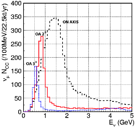
Figure 44: T2K beam neutrino energy spectrum for different off-axis angles, from reference [147]

The aim of what is called phase I (JPARC proton beam power 0.75 MW) are

• In appearance mode a sensitivity (for $\delta=0$) down to 0.008 on $sin^{2}2\theta_{13}$.

  The correlation between $\delta$ and $sin^{2}2\theta_{13}$ sensitivity is shown in Table 13.

• In disappearance mode

  $$\sigma(\Delta m^{2}_{23})=10^{-4}eV^{2}~{}~{}~{}\sigma(sin^{2}\theta_{23})~{}=~{}0.01$$

• And a search for $\nu_{\mu}\rightarrow\nu_{\tau}$ by measurement of neutral current events.

$\delta$	$\sin^{2}2\theta_{13}$
0	8 $\times 10^{-3}$
-$\pi$/2	$3\times 10^{-3}$
$\pi$/2	$2\times 10^{-2}$
$\pi$	$8\times 10^{-3}$

Table 13: $\delta$ vs $sin^{2}2\theta_{13}$ sensitivity for T2K, from reference  [148].

These numbers have been computed for a 5 years run with $5\times 10^{21}$ protons.

Given the low neutrino energy, matter effects will be small.

8.2.2 NO$\nu$A Experiment

The NO$\nu$A experiment has been proposed at Fermilab [64] and is now in an R$\&$D phase on the way for approval. It will be a two detector experiment, with a 810 km baseline, from NUMI beam at Fermilab, at 2.5 degrees off axis. The beam will be at an average momentum of 2.3 GeV. The momentum distribution of interacting neutrinos for various off axis angles is shown in Figure 45.

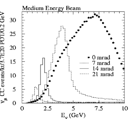
Figure 45: Rates in NO$\nu$A beam, from reference  [64].

The far detector will be made of planes of PVC structures containing liquid scintillator, the close detector will have the same structure followed by a muon catcher. The experiment is on the way of approval.

Initially the experiment will run with a proton beam power of 0.3 MW, then of 0.7 MW, finally of 1.2 MW.

The main aim of the experiment will be the detection of $\nu_{\mu}\rightarrow\nu_{e}$ so the detector will be optimized to separate electron events.

The experiment will be sensitive to the mass hierarchy (see Figure 46) through matter effects. In fact at the first maximum of the oscillation probability we can write (see equation 2):

$$P_{mat}(\nu_{\mu}\rightarrow\nu_{e})=(1+2A)P_{vac}(\nu_{\mu}\rightarrow\nu_{e})$$

Introducing $E_{R}=\Delta m^{2}_{23}/2\sqrt{2}G_{F}N_{e}=E\Delta m^{2}_{23}/|B|$, with $G_{F}$ Fermi constant and $N_{e}$ electron number density, the above expression can be rewritten as

$$P_{mat}(\nu_{\mu}\rightarrow\nu_{e})=(1\pm 2E/E_{R})P_{vac}(\nu_{\mu}\rightarrow\nu_{e}).$$

The sign in front of the $E_{R}$ depending term is + for neutrinos and - for anti-neutrinos. $E_{R}$ will be positive or negative according to the sign of $\Delta m^{2}_{23}$.

In the case of NO$\nu$A, for the normal hierarchy, matter effects increase by about 30$\%$ the oscillation probability or decrease it by the same amount for the inverted one, in the neutrino case. The opposite is true for anti-neutrinos.

As an example Figure 46 shows $P(\nu_{\mu}\rightarrow\nu_{e})$ computed for L=800 km, $\Delta m^{2}_{23}$=0.0025 eV², sin${}^{2}2\theta_{13}$=0.1 and sin${}^{2}2\theta_{23}$=1.

Figure 46: Matter effects in NO$\nu$A experiment.

The probability of oscillation will depend on all the still unknown parameters. The discovery limit for sin${}^{2}2\theta_{13}$ at $\delta$ =0 will be 8$\times 10^{-3}$ or 1.5$\times 10^{-2}$ for normal or inverted hierarchy. The limit will depend on the value of $\delta$ as shown in Figure 47a. Because the anti-neutrinos have an opposite dependence of $\delta$ on sin${}^{2}\theta_{13}$, running neutrinos and anti-neutrinos the correlation will be largely reduced(Figure 47b).

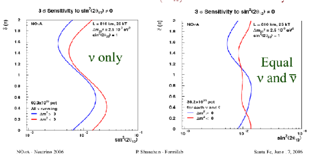
Figure 47: NO$\nu$A sensitivities, $\delta$ versus $sin^{2}(2\theta_{13}$). Left panel neutrino only, right panel neutrinos and anti-neutrinos. Lines represent $\Delta m^{2}_{23}$ positive and negative values, from reference  [149].

9 Long term plans for oscillation experiments

After 2010 the proposed reactor experiments will have improved our knowledge of $\sin^{2}2\theta_{13}$ by about a factor 10 compared to the present limit. Being disappearance experiments they will not give informations on the other missing parameters: mass hierarchy (sign of $\Delta m^{2}_{23}$) and value of $\delta$. These informations will be given by the measurement of P($\nu_{\mu}\rightarrow\nu_{e}$) at an L/E corresponding to the value of $\Delta m^{2}_{23}$ given by the atmospheric neutrinos. First informations will be given by T2K and NO$\nu$A, for which improvements have been proposed.

9.1 Improvements of T2K and NO$\nu$A

T2K experiment

The improvements will consist in

• increase of JPARC proton beam power from 0.75 MW to 4MW

• new far detector Hyper-Kamiokande (HK) with a mass of 0.5 megaton

• run with anti-neutrino beam.

Another possible development proposed is the construction of T2KK [150], a detector in Korea, located at the second oscillation maximum. T2KK will improve the sensitivity on $\delta$, and given the longer distance, matter effects will become considerable with a possibility of determining the mass hierarchy.

NO$\nu$A experiment The upgrade would consists in

a) final proton beam power 1.2 MW

b) a second detector at a different distance possibly using novel technologies (Liquid Argon detector).

At the maximum proton power NO$\nu$A will be able to explore the full phase space for $\delta$ provided sin${}^{2}\theta_{13}\geq 10^{-2}$. If this was the case, in combination with the upgraded T2K experiment, a resolution of 2$\sigma$ would be reached in the determination of mass hierarchy.

9.2 SPL beam to Fréjus

Still in the line of using conventional beams, a proposal has been presented for the Superconducting Linac beam at the Fréjus tunnel. The European project [151] foresees (see Figure 48):

• a super conducting proton Linac with a power of 4 MW, and an energy up to 5 GeV, at CERN;

• a neutrino beam energy of about 300 MeV, optimized to give maximum sensitivity on the far detector located in the Fréjus tunnel (that is at a distance of 130 km from CERN);

• a far detector (MENPHYS [152]) of 500 kton water Cherenkov at a depth 4800 MWE;

• a close detector in the CERN site.

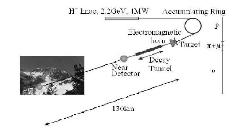
Figure 48: SPL setup, from reference [153].

Competing proposals for the water Cherenkov detector can be found in UNO [154] and Hyper-Kamiokande proposals [148].

In ten years of running a sensitivity of 0.001 at 90$\%$ CL for $\sin^{2}2\theta_{13}$ can be obtained [152].

9.3 Atmospheric neutrinos

A large amount of information could be obtained from an underground large magnetized detector of atmospheric neutrinos. A calorimeter (ICAL) of this type as been proposed by the Indian Neutrino Observatory collaboration (INO) [155]. Comparison of results obtainable in Iron calorimeters and in large water detector can be found in [156]

9.4 New ideas

One of the limiting factors in the measurement of P($\nu_{\mu}\rightarrow\nu_{e}$) is the $\nu_{e}$ contamination in conventional neutrino beams. Novel ideas for high purity beams overcoming this problem have been proposed, these are the Beta Beams and the Neutrino Factories.

9.4.1 Beta Beams:

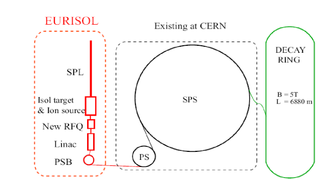
Figure 49: Beta Beam layout, from reference  [157], copyright (2005), with permission from Elsevier.

The Beta Beam idea, introduced by Piero Zucchelli [158], is that $\beta^{+}$ (or $\beta^{-}$) decays, from accelerated radioactive nuclei, produce pure forward $\nu_{e}$ (or $\overline{\nu}_{e}$) beams. Radioactive nuclei producing respectively $\overline{\nu}_{e}$ and $\nu_{e}$ are for example $He^{6}$ and $Ne^{18}$:

$He^{6}\rightarrow Li^{6}+e^{-}+\overline{\nu}_{e}$

$Ne^{18}\rightarrow F^{18}+e^{+}+\nu_{e}$.

According to the type of used radioactive nucleus $\nu_{e}$ or $\overline{\nu}_{e}$ beams will be produced and it will be possible to study $\nu_{e}\rightarrow\nu_{\mu}$ or $\overline{\nu}_{e}\rightarrow\overline{\nu}_{\mu}$ channels.

The characteristics of produced beams will be:

• pure beams with just one flavor

• very intense beam completely known, their energy will be determined by the beta decay energy and Lorentz factor $\gamma$

• flux normalization from the number of the radioactive ions circulating in the ring

• divergence of the beam given by $\gamma$.

A conceptual design of a Beta Beam has been proposed at CERN. A possible layout is shown in Figure 49. The neutrino beam will be sent to the Underground laboratory at the Fréjus tunnel where a megaton Water Cherenkov detector will be deployed, the same proposed for the SPL project. Measurement of $\sin^{2}2\theta_{13}$ down to 0.0004 (at $\delta$ =0) will be possible for 10 years running using appearance and disappearance channels [159].

The physics reach of the CERN Beta Beam + SPL combination is described in [160]. This combination offers the possibility of comparing two beams with the same detector thus reducing the detector related systematic effects. It will be possible to study

• CP violation: comparison of $\nu_{\mu}$ and $\overline{\nu}_{\mu}$ with SPL and $\nu_{e}$ and $\overline{\nu}_{e}$ with Beta Beam

• T violation: comparison of $\nu_{e}\rightarrow\nu_{\mu}$ (Beta Beam) and $\nu_{\mu}\rightarrow\nu_{e}$ (SPL).

9.4.2 Neutrino factories:

The principle of the Neutrino Factory [161] is to produce intense neutrino beams from the decay of muon stored in a ring with long straight sections.

Several projects are under study in Europe, USA and Japan. The results that can be obtained in a Neutrino Factory are described in [162]. It will be possible to reach very small values of sin${}^{2}\theta_{13}$ $\simeq 10^{-4}$ not reachable with other experiments [163].

The proposed energies are of the order of 30-50 GeV implying distances of the order of thousand kilometers and thus requiring massive detectors.

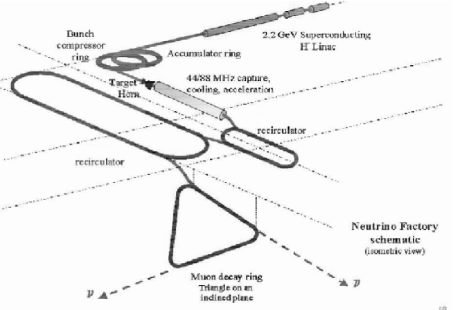
Figure 50: Possible layout of a Neutrino Factory, from reference [164].

A Neutrino Factory project will include (figure 50)

• ion source

• proton accelerator

• pion to muon decay line with beam cooling

• muon accelerator

• muon storage in a decay ring

• neutrino detectors

In Neutrino factories it will be possible to study many channels. A channel (golden channel[165]) that will be studied will consists in the detection of “wrong sign” muons. If we store $\mu^{+}$ they will decay and produce $\overline{\nu}_{\mu}$ and $\nu_{e}$. In the detector $\overline{\nu}_{\mu}$ will produce $\mu^{+}$. $\nu_{\mu}$ from oscillated $\nu_{e}$ will give $\mu^{-}$, which have “wrong sign” with respect to the primary component. Detection of the sign of muons can be achieved using massive magnetized detectors.

The removal of ambiguities and degeneracies has been studied by several authors [144, 145, 146]. It has been shown for example [163] that running on $\nu_{\mu}$ and $\overline{\nu}_{\mu}$ and making experiments with different baselines it will be possible to remove completely ambiguities and degeneracies and that a sensitivity of $\simeq 10^{-4}$ will be reached on sin${}^{2}2\theta_{13}$.

9.5 Comments on future projects

Beta Beams and Neutrino Factories are long term projects. They will require large funding and intensive R$\&$D. On the other hand, conventional beams will give safe results on CP violation only if sin${}^{2}2\theta_{13}\geq 10^{-2}$. Below $10^{-3}$ the only viable solution would be a Neutrino Factory. For a complete discussion of future plans see reference [166] and references in therein.

10 Conclusions

In recent years the evidence for neutrino oscillations has become clear. After 40 years of indications, that did start with R. Davis observation of the solar neutrinos deficit, now we know that neutrinos have mass (although small) and that the mass eigenstates are not the flavor ones. A large amount of experimental data has been collected and many elements of the mixing matrix have been determined. To have a complete description of the mixing matrix the term sin$2\theta_{13}$ needs a better determination, now only upper limits are known, and the phase $\delta$, now completely unknown, must be measured. If sin$2\theta_{13}$ is not too small the way will be open to studies of CP violation in the weak interaction sector, the CP violation term $\delta$ will be accessible.

When the running, approved or on the way of approval, experiments will give their results the future of oscillation experiments will be made more clear and experiments based on novel ideas, Beta Beams and Neutrino Factories, could become necessary.

11 Acknowledgments

We warmly thank Paolo Lipari for encouragement, criticism and discussions. We also gratefully aknowledge the critical reading of P.F Loverre, M. Mezzetto and L. Zanello and the support of C. Mariani in the editing of this paper.

References

References

- [1] Jr. Davis, Raymond, Don S. Harmer, and Kenneth C. Hoffman. Search for neutrinos from the sun. Phys. Rev. Lett., 20:1205–5, 1968.
- [2] B. T. Cleveland et al. Measurement of solar neutrino flux with the homestake detector. Astrophys. J., 496:505–21, 1998.
- [3] W.J.N. Abdurashitov et al. Measurement of neutrino capture rate in metallic gallium. Phys. Rev. C, 60:0055801–34, (eprint astro–ph/9907113), 1999.
- [4] W. Hampel et al. Gallex solar neutrino observation. Phys. Lett. B, 447:127–7, 1999.
- [5] W. Altmann et al. Complete results of five years of gno solar neutrino observations. Phys. Lett. B, 616:174–22,(eprint hep–ex/0504037), 2005.
- [6] S. Fukuda et. Solar neutrino data covering solar cycle 22. Phys. Rev. Lett., 77:1683–4, 1996.
- [7] J. Hosaka et al. Solar neutrino measurements in super-kamiokande-i. Phys. Rev. D, 73:112001–33,(eprint hep–ex/0508053), 2006.
- [8] B. Aharmim et al. Determination of nue and total b-8 solar neutrino fluxes with the sudbury neutrino observatory,phase 1 data set. Phys. Rev. C, 75:045502–78,(eprint nucl–ex/0610020), 2007.
- [9] T. Araki et al. Measurement of neutrino oscillations with kamland: Evidence for spectral distorsion. Phys. Rev. Lett., 94:081801–5,(eprint hep–ex/0406035), 2005.
- [10] Y. Fukuda et al. Measurement of the solar neutrino flux from super-kamiokande first 300 days. Phys. Rev. Lett., 81:1158–1162, 1998.
- [11] Y.Fukuda et al. Evidence for oscillations of atmospheric neutrinos. Phys. Rev. Lett, 81:1562–6 (hep–ex/9807003), 1998.
- [12] M. Ambrosio et al. Measurement of atmospheric neutrino oscillations, global analysis of data collected with the macro detector. Euro Phys. Journal, 36:323–16, 2004.
- [13] M. Sanchez et al. Measurement of l/e distribution in soudan2 and their interpretation as neutrino oscillations. Phys. Rev. D, 68:113004–29,(eprint(hep–ex/0307069), 2003.
- [14] M.H. Ahn et al. Mesurement of neutrino oscillations by the k2k experiment. Phys. Rev D., 74:072003–49,(hep–ex/0606032), 2006.
- [15] P.Adamson et others. Charge separated atmospheric neutrino induced muons in the minos detector. Phys. Rev D., 75:092003–14,(eprint hep–ex/0701045), 2007.
- [16] T. Kajita. discovery of neutrino oscillations. reports on Progress in Physics, 69:1607–29, 2006.
- [17] B. Pontecorvo. Mesonium and anti-mesonium. Sov. Phys. JETP, 6:429,(Zh.Eksp.Teor,33,549,1957), 1957.
- [18] B. Pontecorvo. Inverse beta processes and nonconservation of lepton charge. Sov. Phys. JETP, 7:172–02, (Zh.Eksp.Teor.fiz,34,247,1957), 1958.
- [19] B. Kaiser. neutrino mass mixing and oscillations. electronic preprint hep-ph/0104147, page 26, 2001.
- [20] A. Alberico and S.M. Bilenky. neutrino oscillations mass and mixing. Phys. Part. Nucl, 35:297–67,(eprint hep–ph/0306239), 2003.
- [21] C. Giunti and M.Lavader. neutrino mixing. electronic preprint Hep-ph/0310238, page 53, 2003.
- [22] A. Strumia and F.Vissani. neutrino mass mixing and oscillations. electronic preprint Hep-ph/0606054, page 218, 2006.
- [23] M. C. Gonzalez-Garcia and J. Nir. Neutrino masses and mixing :evidence and implications. Rev.Mod.Physics, 75:345–127 (eprint hep–ph/0202058), 2003.
- [24] P.Lipari. Introduction to neutrino physics. Cern yellow paper 2003-003, pages 115–86, 2003.
- [25] H. V. Klapdor-Kleingrothous et al. Evidence for neutrinoless double beta decay. Mod. Phys. Lett., A16:2409–12,(hep–ph/0201231), 2001.
- [26] E. Fiorini. Double decay and majorana neutrinos. Twelfth International workshop on neutrino telescopes (Venice, Italy, 6-9 March 2007), pages 459–17, 2007.
- [27] A. Vogel and A.Piepke. Review of Particle Physics: introduction to neutrino properties. Journal of Physics G, 33:472, 2006.
- [28] U. Seliok et al. Cosmological parameters analysis. Phys. Rev., D71:103515–20,(eprint Astro–ph/0407372), 2005.
- [29] S.P. Mikheyev and A.Y. Smirnov. Resonant amplification od oscillations im matter and spectroscopy of solar neutrinos. Sov. Jour. Nucl. Phys., 42:913–5, 1985.
- [30] L. Wolfenstein. Neutrino oscillations in matter. Phys. Rev., D17:2369–19, 1978.
- [31] T.K. Kuo and M.Pantaleone. Neutrino oscillations in matter. Rev. of Modern Phys., 61:937–180, 1989.
- [32] V. Barger et al. matter effects in three-neutrino oscillations. Phys. Rev D., 22:2118–27, 1980.
- [33] J. Arafune et al. Cp violation and matter effects in long baseline neutrino oscillation experiments. Phys. Rev. D, 55:1653–6 (eprint hep–ph/9703351), 1997.
- [34] B. Richter. Conventional beams or neutrino factories:the next generation of accelerator neutrino experiment. Electronic eprint hep-ph/0008222, page 7, 2000.
- [35] M. Freund et al. Systematic search of neutrino factory parameter space. Nucl.Phys., B651:331–28,( eprint hep–ph/0105071), 2001.
- [36] A.Cervera et al. Golden measurement in a neutrino factory. Nucl. Phys., B579:255–10,(eprint hep–ph/0002108), 2000.
- [37] P. Adamson et al. A study of muon neutrino disappearence using the fermilab main injector neutrino beam. electronic preprint arXiv:0711.0769, page 57, 2007.
- [38] E. Eskut et al. Final results on oscillation from the chorus experiment. Nucl. Phys. B, 793:326–17,(eprint arXiv:0710.3361), 2008.
- [39] P. Astier et al. Final nomad results on muon-neutrino and electron-neutrino to tau-neutrino oscillations including a new search for tau-nutrino appearence using hadronic tau decays. Nucl.Phys. B, 611:3–33,(eprint hep–ex/0106102), 2001.
- [40] Donald Clayton. Principles of Stellar Evolution and Nucleosynthesis. The University of Chicago Press, 1983.
- [41] j. Bahcall et al. Standard Solar Models and the Uncertainties in Predicted Capture Rates of Solar Neutrinos. Rev. Mod. Phys., 54:767, 1982.
- [42] J.Bahcall, A.M. Serenelli, and S.Basu. New solar opacities, abundances, helioseismology, and neutrino fluxes. Astrophys. J., 621:L85–211 ,(eprint astro–ph/0412440), 2005.
- [43] John N. Bahcall and A.M. Serenelli. How do uncertanties in the surface chemical abandance of the sun affect the predicted solar neutrino fluxex. Astrophys. J., 626:530–47,(eprint astro–ph/0412096), 2005.
- [44] B.T. Cleveland V. N. Gavrin. radiochemical neutrino expeiments. electronic preprint nucl-ex/0703012, page 8, 2007.
- [45] M. Apollonio et al. Search for neutrino oscillations on a long base-line at the chooz nuclear power station. Eur. Phys. J., C27:331–44,( eprint hep–ex/0301017), 2003.
- [46] M. Honda M et al. Calculation of atmospheric neutrino flux using the interaction model calibrated with atmospheric muon data. Phys. Rev., D75:043006–(eprint astro–ph/0611418), 2007.
- [47] M. Honda et al. A new calculation of the atmospheric neutrino flux in a 3- dimensional scheme. Phys. Rev. D, 70:043008–32 (eprint astro–ph/0404457), 2004.
- [48] M. Honda et al. Calculation of the flux of atmospheric neutrinos. Phys. Rev., D52:4985–52, 1995.
- [49] G.Battistoni t al. The fluka atmospheric neutrino flux calculation. Astropart. Phys., 19:269–22,(eprint hep–ph/0207035), 2003.
- [50] A. Ferrari and P. Sala. The physics of high energy reactions. CERN-ATL-PHYS-97-113, 1997.
- [51] V. Agrawal et al. Atmospheric neutrino flux above 1 gev. Phys. Rev. D, 53:1314–20, (eprint hep–ph/9509423), 1996.
- [52] L. Casagrande et al. The alignment of the cern west area neutrino facility. CERN-96-06, 1996.
- [53] J.A. Holder et al. A detector for high energy neutrino interactions. Nucl. Istr. and Meth., 148:235–34, 1977.
- [54] A. N.Diddens et al. A detector for neutral current interactions of high-energy neutrinos. Nucl. Inst. and Meth. A, 178:127–27, 1980.
- [55] K. De winter et al. A detector for study of neutrino electron scattering. Nucl. Istr. and Meth., 278:670–27, 1989.
- [56] E. Eskut et al. The chorus experiment to search for num nutau oscillations. Nucl. Inst. and Meth. A, 401:7–74, 1997.
- [57] J. Altegoer et al. The nomad experiment at the cern sps. Nucl. Inst. and Meth. A, 404:96–37, 1998.
- [58] P.Astier et al. Prediction of neutrino fluxes in the nomad experiment. Nucl. Inst. and Meth. A, 515:800–8 (e–Print hep–ex/0306022), 2003.
- [59] F. Dydak et al. A search for muon-neutrino oscillations in the deltam*2 range 0.3ev**2 to 90 ev**2. Phys. Lett.B, 134:281–11, 1984.
- [60] F. Bergsma et al. A search for oscillations of muon-neutrino in an experiment with l/e approximately 0.7-km/gev. Phys. Lett.B, 142:103–16, 1984.
- [61] C.Angelini et al. New experimental limits on muon-neutrino to electron-neutrino oscillations. Phys. Lett. B, 179:307–18, 1986.
- [62] D. Michael et al. The minos experiment. Nucl. Phys. Proc. Suppl., 118:189–8, 2003.
- [63] D. Beavis et al. Long baseline neutrino oscillation experiments at the ags. Report No. BNL-32459, page 10, 1995.
- [64] D. Ayres et al. Nova proposal to build a 30 kiloton off-axis detector to study neutrino oscillations in the fermilab numi beamline. Fermilab-Proposal-0929, hep-ex/0503053v1, 2005.
- [65] A. Aguilar et al. Evidence for neutrino oscillations from the observation of anti-neutrino(electron) appearence in a anti-neutrino beam. Phys. Rev. D, 64:112007–44,(eprint hep–ex/0104049), 2001.
- [66] S. J. Barish et al. Study of neutrino interactions in hydrogen and deuterium. Description of the experiment and study of the reaction neutrino . Phys. Rev., D16:3103–19, 1977.
- [67] S. Bonetti et al. Study of quasielastic reactions of neutrino and anti-neutrino in gargamelle. Nuovo Cim., A38:260–10, 1977.
- [68] S. Ciampolillo et al. Total cross-section for neutrino charged current interactions at 3 GeV and 9 GeV. Phys. Lett., B84:281–9, 1979.
- [69] N. Armenise et al. Charged current elastic anti-neutrino interactions in propane. Nucl. Phys., B152:365–11, 1979.
- [70] S. V. Belikov et al. Quasielastic neutrino and anti-neutrinos scattering: total cross-sections, axial vector form-factor. Z. Phys., A320:625–20, 1985.
- [71] G. M. Radecky et al. Study of single pion production by weak charged currents in low-energy neutrino deuterium interactions. Phys. Rev., D25:1161–13, 1982.
- [72] T. Kitagaki et al. Charged current exclusive pion production in neutrino deuterium interactions. Phys. Rev., D34:2554–12, 1986.
- [73] P. S. Auchincloss et al. Measurement of the inclusive charged current cross-section for neutrino and anti-neutrino scattering on isoscalar nucleons. Z. Phys., C48:411–23, 1990.
- [74] J. P. Berge et al. Total neutrino and anti-neutrino charged current cross- section measurements in 100 gev, 160 gev and 200 gev band beams. Z. Phys., C35:443, 1987.
- [75] V. B. Anikeev et al. Total cross-section measurements for muon-neutrino, anti- muon-neutrino interactions in - 30 gev with IHEP-JINR neutrino detector. Z. Phys., C70:39–7, 1996.
- [76] A. S. Vovenko et al. Energy dependence of total cross-sections for neutrino and anti-neutrino interactions at energies below 35 GeV. Sov. J. Nucl. Phys., 30:528–11, 1979.
- [77] D. MacFarlane et al. Nucleon structure functions from high-energy neutrino interactions with iron and QCD results. Z. Phys., C26:1–27, 1984.
- [78] N.J. Baker et al. Total cross-sections for muon-neutrino n and muon-neutrino p charged current interactions in the 7-ft bubble chamber. Phys. Rev., D25:617–4, 1982.
- [79] J. Bahcall et al. Standard neutrino spectrum from decay. Phys. Rev., C54:411–13,( eprint nucl–th/9601044), 1996.
- [80] R. J. Davis, D. S. Hamer, and K. C. Hoffman. Search for neutrinos from the sun. Phys. Rev. Lett., 20:1205, 1968.
- [81] J. Bahcall and N.Bahcall. Present status of the theoretical predictions for the cl solar neutrino experiment. Phys. Rev. Lett., 20:1209–5, 1968.
- [82] S. Hatakeyama et al. Measurement of the flux and zenith angle distribution of upward going muons in kamiokande i+ii. Phys. Rev. Lett, 81:2016–4, 1998.
- [83] Y. Ashie et al. Measurement of atmospheric neutrino oscillation parameters by Super-Kamiokande I. Phys. Rev. D, 71:112005–35, 2005.
- [84] J. P. Cravens et al. Solar neutrino measurements in Super-Kamiokande II. Phys. Rev. D, to be published, 2007.
- [85] Y. Takeuchi et al. Low-energy neutrino observation at Super-Kamikande III . Proceedings of the TAUP conference 2007 (Sendai, Japan, 11-15 September 2007), at press, 2007.
- [86] B. Aharmim et al. Electron energy spectra,fluxes and daynight asymmetry of b8 solar neutrinos from measurements with nacl dissolved in the heavy water of the sudbury neutrino observatory. Phys. Rev. C, 72:055502–45,(nucl–ex/0502021), 2005.
- [87] J. Bahcall, A.M Serenelli, and S. Basu. Solar models:current epoch and time dependence, neutrinos and helioseismological properties. Astrophys. J., 555:990–22,(eprint astro–ph/0010346), 2001.
- [88] S.N. Ahamed et al. Measurement of the total b-8 neutrino flux at sno with enhanced nc sensitivity. Phys. Rev. Lett., 92:181301–5,(eprint nucl–ex/0309004), 2004.
- [89] A.B. McDonald. Solar neutrinos sno and snolab. Phys.Scripta T, 127:10–13, 2006.
- [90] C. Arpesella et al. First real time detection of solar neutrinos by borexino. Phys. Lett., 658B:101–7 ,(eprint arXiv:0708.2251v1), 2007.
- [91] K. Nakamura. Particle data group. journal of physics G, 33:485–7, 2006.
- [92] G.L. Fogli et al. Global analysis of three flavor neutrino masse and mixing and refereces therein. Progr.Part.Nucl.Phys, 57:742–63,(eprint hep–ph/0506083), 2006.
- [93] M.B. Smy et al. Precise measurement of the solar neutrino day-nightand seasonal variations in in super-kamiokande-i. Phys. Rev. D, 69:0011104–33,(eprint hep–ex/0508053), 2004.
- [94] C.Bemporad, G.Gratta, and P.Vogel. Reactor based neutrino oscillation experiments. Rev.Mod.Phys, 74:297–35, (eprint hep–ph/0107277), 2002.
- [95] H. Kwon et al. Search for neutrino oscillation at fission reactor. Phys.Rev D, 24:1097–15, 1981.
- [96] G.S. Vidyakin et al. Limitations on the characteristic of neutrino oscillation. Jept Lett., 59:390–4, 1994.
- [97] V. Zacek et al. Search for neutrino oscillation at the nuclear power reactor at goesgen. Phys.Rev D, 34:2621–16, 1986.
- [98] B. Achkar et al. Comparison of anti-neutrino reactor spectrum with the bugey-3 measurements. Phys. Lett. B, 374:243–12, 1996.
- [99] F. Boehm et al. Final results of the palo verde neutrino oscillation experiment. Phys. Rev. D, 64:112001–11, (eprint hep–ex/0107009), 2001.
- [100] K. Eguci et al. First results from kamland: Evidence for reactor antineutrino disappearance. Phys. Rev. Lett., 90:021802–6,(eprint hep–ex/0212021v1), 2003.
- [101] V. D. Barger et al. neutrino decay as an explanation of atmospheric neutrino observation. Phys. Rev. Lett., 82:2640–5,(eprint astro–ph/9810121), 1999.
- [102] E. Lisi et al. Probing possible decoherence in atmospheric neutrino oscillations. Phys. Rev. Lett., 85:1166–4,(eprint hep–ph/0002053), 2000.
- [103] K. Heeger. recent neutrino reactor experiments reactor neutrino experiments. Proceedings of the TAUP conference 2007 (Sendai, Japan, 11-15 September 2007), at press, 2007.
- [104] D. Becker-Szendy et al. A serach for neutrino oscillations with the imb detector. Phys. Rev. Lett., 69:1010–3, 1992.
- [105] Y. Fukuda et al. Atmospheric muon-neutrino and electron-neutrino ratio. Phys. Lett. B, 335:237–9, 1994.
- [106] Y. Ashie et al. Measurement of atmospheric neutrino oscillation parameters by super-kamiokande i. Phys. Rev. D, 71:112005–31,(eprint hep–ex/0501064), 2005.
- [107] T. Kaijta and P.Lipari. Atmospheric neutrinos and oscillations. Comptes Rendus de Physique, 6:738–749, 2005.
- [108] J. Hosaka et al. three flavour neutrino oscillation analysis of atmospheric neutrino in super-kamiokande. Phys. Rev. D, 74:032002–9,(eprint hep–ex/0604011), 2006.
- [109] Y. Ashie et al. Evidence for an oscillatory signature in atmospheric neutrino oscillations. Phys. Rev. Lett, 93:101801–6,(eprint hep–ex/0404034), 2004.
- [110] P.Adamson et others. first observation of separated atmospheric nu(mu) and antinu(mu) in the minos detector. Phys. Rev D., 73:092003–14,(eprint hep–ex/0512036), 2006.
- [111] B. Pontecorvo. electron and muon neutrino. Sov. Phy.Jept,, 10:1236–5,(Zh Exp Teor fiz 37,1751,1957), 1960.
- [112] M. Schwartz. Feasibility of using high energy neutrinos to study weak interactions. Phys. Rev. Lett., 4:306–2, 1960.
- [113] G. Danby. observation of high energy neutrino reactions and the existence of two kind of neutrino. Phys. Rev. Lett., 9:36–5, 1962.
- [114] E. Bellotti et al. A preliminary limit om neutrino oscillations in gargamelle experiments. Lettere Nuovo Cimento, 17:553–3, 1976.
- [115] O. Erriquez et al. Limits on neutrino oscillations from a study of electron neutrino charged currents interactions. Phys. Lett.B, 102:73–15, 1981.
- [116] N. J. Baker et al. Experimental limits on neutrino oscullations. Phys. Rev. Lett., 47:1576–5, 1981.
- [117] L.A. Ahrens et al. a new limit on the strenght of mixing between muon neutrino and electron neutrino. Phys Rev D, 31:272–18 (eprint: hep–ex/9908056), 1987.
- [118] B. Blumenfeld et al. Search for numu nue oscillations. Phys. Rev. Lett., 62:2237–5, 1989.
- [119] D. H. Harris et al. Precise calibration of the nutev detector. Nucl. Inst. and Meth. A, 447:377–39, 2000.
- [120] F. Bergma et al. Search for neutrino oscillations. Z. Phys.C, 40:171–237, 1988.
- [121] L. Borodovsky et al. Search for mu-neutrino e-neutrino oscillations in a wide band neutrino beam. Phys. Rev. Lett., 68:274–8, 1992.
- [122] L.A. Harens et al. Search for neutrino oscillations. Phys. Rev. D, 31:2732–2750, 1985.
- [123] P. Vilain et al. Search for nuon to electron neutrino oscillations. Z.Phys. Rev. C, 64:539–5, 1995.
- [124] S. Avvakumov et al. Search for muon-neutrino electron-neutrino and muon-antineutrino electron-antineutrino oscillation at nutev. Phys. Rev. Lett., 89:011804–4, (eprint hep–ex 0203018), 2002.
- [125] P. Astier et al. Search for nuon to electron neutrino oscillations in the nomad experiment. Phys. Lett. B., 570:539–19,(eprint hep–ex/0306037), 2003.
- [126] N. Ushida et al. limits on oscillations. Phys. Rev. Lett., 57:2897–5, 1986.
- [127] B. Armbruster et al. Upper limits for neutrino oscillations muon-antineutrino to electron-antineutrino fro muon decay at rest. Phys. Rev. D, 65:112001–42 (eprint: hep–ex/0203021), 2002.
- [128] A.A. Aguilar Arevalo et al. A search for electron neutrino apparance at the delta m**2 1-ev**2 scale. Phys. Rev. Lett., 98:231801–7,(eprint arXiv:0704.1500), 2007.
- [129] Yamamoto et al. Improved search for nu-mu to nu-e oscillation in a long baseline experiment. Phys. Rev. Lett., 96:181801–5 (eprint: hep–ex/0603004, 2006.
- [130] D. Michael et al. Observation of muon neutrino disappearence with the minos detector at the numi beam. Phys.Rev.Lett, 97:191801–6,(eprint hep–ex/0607088), 2006.
- [131] A. Blake et al. New results of the Minos experiment. Proceedings of the TAUP conference 2007 (Sendai, Japan, 11-15 September 2007), at press, 2007.
- [132] M. Guler et al OPERA Collaboration. Experiment proposal. CERN-SPSC-2000-028, 2000.
- [133] M. Komatsu et al. Sensitivity to theta(13) of the cern to gran sasso beam. j of Physics G, 29:243–13 (eprint: hep–ph/0210043), 2003.
- [134] R. Acquafredda et al. First events from the cngs neutrino beam detected by the opera experiment. New.J.Phys, 8:303–12 ( eprint: hep–ex/0611023), 2006.
- [135] A.Ariga. Opera experiment and emulsion tecnique. Proceedings of Nufact 2007 (Okayama, Japan, 6-11 August 2007), pages 175–4, 2007.
- [136] M. Maltoni et al. Global fits to neutrino oscillations. New Journal of physics, 6:122–39 (eprint: hep–ph/0405172), 2004.
- [137] T.Schwetz. Global fits to neutrino oscillations data. Physics Scripta, t127:1–5 (eprint: hep–ph/0606060), 2006.
- [138] N. Cabibbo. Time reversal violation in neutrino oscillations. Phys. Lett, 72:333–8, 1978.
- [139] J.C. Anjos et al. Angra dos reis reactor neutrino oscillatio experiment. Brasilian Journal of Physics, 36:1118–6, 2006.
- [140] Xineng Guo et al. A precise measurement of the neutrino mixing angle theta(13) using reactor antineutrinos at daya bay. electronic preprint hep-ex/0701029, page 162, 2007.
- [141] F.Ardellier. Double chooz, a search for neutrino mixing angle theta-13. electronic preprint hep-ex/0606025, page 173, 2006.
- [142] M. Aoki et al. High accuracy neutrino measurement from the kashiwazaki-kariva nuclear power station. electronic preprint hep-ex/0607013, page 85, 2006.
- [143] K.K.Joo et al. Reno project. http://neutrino.snu.ac.kr/RENO/INTRO/intro.html, 2007.
- [144] V. Barger, D. Marfatia, and K. Whisnant. Breaking eight-fold degeneracies in neutrino CP violation, mixing, and mass hierarchy. Phys. Rev., D65:073023–35,(hep–ph/0112119), 2002.
- [145] J. Burguet-Castell, M. B. Gavela, J. J. Gomez-Cadenas, P. Hernandez, and Olga Mena. On the measurement of leptonic CP violation. Nucl. Phys., B608:301–18,(eprint hep–ph/0103258), 2001.
- [146] P. Migliozzi. Eightfold degeneracy studies with a standard beta-beam and a super-beam facility. Nucl. Phys. Proc. Suppl., 149:182–3 (eprint: hep–ph/0406132), 2005.
- [147] Y.Itow et al. Jhf kamioka project. electronic preprint hep-ex/0106019, 2001.
- [148] K. Nishikawa. Status of j-park facility and the t2k experiment. Twelfth International workshop on neutrino telescopes (Venice, Italy, 6-9 March 2007), pages 197–4, 2007.
- [149] P. Shana. nova sensitivities. trasparencies of Neutrino 2006, 2006.
- [150] T. Kajita. Updating the futur long baseline experiment with the kamioka-korea two detector setup. Twelfth International workshop on neutrino telescopes (Venice, Italy, 6-9 March 2007), pages 211–12, 2007.
- [151] M. Mezzetto. Physics potential of the spl superbeam. Journal of Phisics G, 29:1781–4, (eprint hep–ex/0302005, 2003.
- [152] A. De Bellefon et al. A large scale water cerenkov detector at frejus. electronic preprint hep-ex/0607026, page 33, 2006.
- [153] J E Campagne and A Cazes. The and sensitivities of the spl-fréjus project revisited. Technical Report CARE-NOTE-2004-031-BENE, CARE, 2004.
- [154] C.K.Jung et al. Feasiblity of a next generation underground cherenkov detector:uno. electronic preprint hep-ex/0005046, page 6, 200.
- [155] M.S. Athar et al. India based neutrino observatory,project report. INO-2006-01, page 230, 2006.
- [156] S. Chubey. What we can learn from atmospheric neutrinos. electronic preprint hep-ph/0609182, page 7, 2006.
- [157] M. Mezzetto. SPL and beta beams to the Frejus. Nucl. Phys. Proc. Suppl., 149:179–3, 2005.
- [158] P. Zucchelli. A novel concept for anti-nue ,nue factory,the beta beam. Phys. Lett. B, 532:166–7, 2002.
- [159] M. Mezzetto. Physics potential of the gamma = 100,100 beta beam. Nucl. Phys. B, 155:214–4 ,(eprint hep–ex/0511005), 2006.
- [160] M. Mezzetto. Physics reach of the beta beam. J. Phys. G, 29:1771–6,(eprint hep–ex/0302007), 2003.
- [161] S. Geer. Neutrino beams from muon storage ring. Phys Rev D, 57:6989–6997, 1998.
- [162] M. Apollonio et al. Oscillation physics with a neutrino factory. electronic preprint hep-ph/0210192, page 105, 2002.
- [163] P. Huber and W. Winter. Neutrino factories and the ’magic’ baseline. Phys. Rev., D68:037301–4,(eprint hep–ph/0301257), 2003.
- [164] P. Gruber et al. The study of a european neutrino factory complex. Technical Report CERN-PS-2002-080-PP. CERN-NEUTRINO-FACTORY-NOTE-122. CERN-NUFACT-NOTE-122, CERN, Geneva, Dec 2002.
- [165] A. Donini et al. Summary of golden measurement at a neutrino factory. Nucl. Inst. and Meth. A, 472:403–5, (eprint hp–ph/0007281), 2000.
- [166] A. Blondel. future neutrino oscillations facilities: priorities and open issues. Nucl. Phys. B (proc suppl), 155:131–12,(eprint hep–ph/0601158), 2006.