Hanle effect in the solar Ba ii D2 line: a diagnostic tool for chromospheric weak magnetic fields

Abstract

Context. The physics of the solar chromosphere depends in a crucial way on its magnetic structure. However there are presently very few direct magnetic field diagnostics available for this region.

Aims. Here we investigate the diagnostic potential of the Hanle effect on the Ba ii D2 line resonance polarization for the determination of weak chromospheric turbulent magnetic fields.

Methods. The line formation is described with a non-LTE polarized radiative transfer model taking into account partial frequency redistribution with an equivalent two-level atom approximation, in the presence of depolarizing collisions and the Hanle effect.We investigate the line sensitivity to temperature variations in the low chromosphere and to elastic collision with hydrogen atoms. We compare center-to-limb variations of the intensity and linear polarization profiles observed at THEMIS in 2007 to our numerical results.

Results. We show that the line resonance polarization is very strongly affected by partial frequency redistribution effects both in the line central peak and in the wings. Complete frequency redistribution cannot reproduce the polarization observed in the line wings. The line is weakly sensitive to temperature differences between warm and cold components of the chromosphere. The effects of elastic collisions with hydrogen atoms and of alignment transfer due to multi-level coupling with the metastable ${}^{2}D_{5/2}$ levels have been studied in a recent paper showing that they depolarize the ${}^{2}P_{3/2}$ level of the line. In the conditions where the line is formed we estimate the amount of depolarization due to this mechanism as a factor of 0.7 to 0.65. If we first neglect this effect and determine the turbulent magnetic field strength required to account for the observed line polarization, we obtain values between 20 G and 30 G. We show that this overestimates the magnetic strength by a factor between 1.7 and 2. Applying these correction factors to our previous estimates we find that the turbulent magnetic field strength is between 10 G and 18 G.

Conclusions. Because of its low sensitivity to temperature variations, the solar Ba ii D2 line appears as a very good candidate for the diagnosis of weak magnetic fields in the low chromosphere ($z\geq 900$ km) by means of the Hanle effect.

1 Introduction

Magnetic fields play a crucial role in the physics of the solar chromosphere (Innes et al. 2005), however we lack direct reliable diagnostic tools for the measurement of the field in this region. The Zeeman effect on chromospheric lines is not easily interpreted because most of them are broad and formed under non-LTE conditions. Moreover, the field strength decreases from the photosphere to the chromosphere and the physical conditions are highly inhomogeneous so that the measurements of the Zeeman polarization requires high spatial and spectral resolution. In this context, the Hanle effect can provide a valuable diagnostic tool because it is sensitive to weaker fields than the Zeeman effect and it does not average out in the presence of unresolved mixed polarity fields. The Hanle effect affects lines formed by scattering of photons under anisotropic illumination by modifying their linear resonance polarization; it is thus likely to occur in chromospheric conditions.

Here we investigate the diagnostic potential of the resonance line of ionized barium at 455.4 nm. Its linear polarization has been recorded outside active regions by several authors using different instruments (Stenflo and Keller 1997, Malherbe et al. 2006). The observations that we show in this paper were obtained at THEMIS in July 2007.

Theoretical works dedicated to the physical interpretation of these observations are still in progress. A very comprehensive study of the magnetic sensitivity of the Ba ii D1 and D2 lines, fully taking into account the hyperfine structure of the odd isotopes of barium, has been published by Belluzzi et al. (2007). However, this work, devoted to the investigation of the various physical mechanisms which can play a role in the line polarization, does not take into account radiative transfer effects. The line is modeled under the last scattering approximation and the anisotropy of the radiation field which gives rise to resonance polarization is chosen ad-hoc. Here we adopt a complementary approach: we focus on the radiative transfer effects and neglect the hyperfine structure of the odd isotopes of Ba ii. This will not allow us to recover the well-known triple peak structure of the line polarization profile, but we shall concentrate on the central polarization peak, which is due to the even isotopes. This approach is justified by the study of Belluzzi et al., which has shown that the central polarization peak is sensitive to the Hanle effect of weak turbulent magnetic fields, whereas the two secondary peaks due the odd isotopes are not. Moreover, in the line wings the linear polarization degrees of the even and odd isotope components are identical. In other words, the linear polarization in the line wings may be computed ignoring the hyperfine structure of the odd isotopes.

In the absence of hyperfine structure the ground level of the even isotopes of Ba ii is non polarizable by radiation anisotropy; this is no longer true for the odd isotopes. This might affect the line polarization at the wavelengths of the two secondary peaks due to the odd isotopes, but not in the central peak nor in the line wings. Furthermore, it is very likely that any ground level polarization would be destroyed by elastic collisions with hydrogen atoms, as is the case for the metastable ${}^{2}D_{5/2}$ levels (see Derouich 2008).

In Sect. 2 we present the observations that we performed at THEMIS together with some comments on data reduction. In Sect. 3 we explain our non-LTE radiative transfer modeling of the line, taking into account partial frequency redistribution and the Hanle effect due to turbulent magnetic fields. We show that partial frequency redistribution plays an important role in the resonance polarization profiles obtained close to the solar limb. In Sect. 4 we investigate the diagnostic potential of the line polarization. We first test its sensitivity to temperature variations in the low chromosphere, because the temperature may be quite inhomogeneous and time-dependent in this layer (see Avrett 1995). We use two different models of the quiet solar atmosphere, namely the standard average FALC model (Fontenla, Avrett and Loeser 1993) and the FALX model (Avrett 1995) derived from infrared measurements in the CO molecule, which is significantly cooler in the low chromosphere. We also deal with the effect of the elastic collisions which both broaden and depolarize the line. We show that at the altitude where the line is formed, the hydrogen density is low enough not to play a significant role in the line broadening. The line depolarization by elastic collisions with hydrogen atoms has been studied in detail by Derouich (2008). This study has shown that in low density media the depolarization of the ${}^{2}P_{3/2}$ level is not due to the relaxation of the alignment but to alignment transfer between the ${}^{2}P_{3/2}$ level and the metastable ${}^{2}D_{5/2}$ levels. The line polarization is thus overestimated if one neglects multi-level alignment transfer. As no fully consistent multi-level polarized transfer code is presently available, we propose to compute the line polarization with an equivalent two-level atom model and to take into account multi-level alignment transfer effects by introducing a correction factor to our results. We give this correction factor for typical values of the hydrogen density in the low chromosphere above $z=900$ km. Then, we show how the center-to-limb variations of the linear polarization in the central peak of the line may be used to investigate weak turbulent magnetic fields in the low chromosphere of the Sun.

2 Observations and data reduction

The limb polarization of Ba ii 4554 Å was acquired with the THEMIS telescope on 27 July 2007. The observation was performed at the North Pole, and the slit was placed parallel to the limb, at a series of limb distances (4, 10, 20, 40 and 80 arcsec). For the short limb distances (4 and 10 arcsec), the limb distance was determined in the slit-jaw images. For the larger limb distances, the limb distance was manually allocated by using the pursuit tool of the telescope. The THEMIS telescope was operating in the MTR-grid mode, and the data were averaged along the slit. The polarization was measured by applying the beam-exchange technique, and the data reduction was done following Bommier & Rayrole (Bommier-Rayrole-02 (2002)) and Bommier & Molodij (Bommier-Molodij-02 (2002)), except for the fact that the THEMIS polarimeter was later modified, now allowing beam-exchange for all the 3 polarization Stokes parameters individually. No significant signal was detected on Stokes $U$ and $V$. The observation results for Stokes $Q$ are reported in Fig. 1. The continuum polarization was adjusted to the theoretical value given by Fluri & Stenflo (Fluri-Stenflo-99 (1999)).

Figure 1: Observation of the limb polarization of Ba  ii 455.4 nm for a series of limb distances: from top to bottom, the slit was positioned 4, 10, 20, 40 and 80 arcsec inside the limb, and parallel to it. The data have been averaged along the slit.

3 Non-LTE line modeling

In order to compute the line intensity and polarization profiles both without and with the Hanle effect we use the same procedure as the one described by Faurobert-Scholl (1992). In a first step we solve the statistical equilibrium equations for the populations of the atomic levels, coupled to the line and continuum transfer equations, neglecting the polarization. This provides us with the optical depth in the line of interest and with multi-level coupling terms in its source function. In a second step, we compute the line intensity and polarization with an equivalent two-level approach. This two-step method relies on the fact that the line linear polarization is weak enough not to play a role in the statistical equilibrium of the atomic levels and on the hypothesis that the alignment of the ${}^{2}P_{3/2}$ upper level is only due to optical pumping from the unpolarized ground level, partially destroyed by elastic collisions, but not affected by radiative coupling with other atomic levels. However in the case of the Ba ii D2 line we have to take into account depolarizing effects due to alignment transfer between the ${}^{2}P_{3/2}$ level and the metastable ${}^{2}D_{5/2}$; this is done by introducing a correction factor on the line polarization obtained from our equivalent two-level modeling.

The barium atom has odd and even isotopes with slightly different atomic structures. The 134, 136 and 138 even isotopes (82.1% of the total number density) have no nuclear spin, i.e. no hyperfine structure, whereas the 135 and 137 odd isotopes have a nuclear spin $I=3/2$; the hyperfine structure of their fundamental level is detectable (Rutten 1978), but we do not consider it here, as we deal only with the central polarization peak due to the even isotopes. Figure 2 shows the atomic model that we use, together with the allowed radiative transitions.

3.1 Polarization radiative transfer equation and redistribution matrix in the presence of a weak magnetic field

The polarized radiative transfer equation that we solve for the 455.4 nm resonance line is written

$$\mu{\partial{\bf I}(\nu,{\bf n},z)\over\partial\tau_{\nu}}={\bf I}(\nu,{\bf n},z)-{\bf S}(\nu,{\bf n},z),$$ (1)

where $\mu$ is the cosine of the heliocentric angle of the line of sight, ${\bf I}$ is the 2-component vector $(I,Q)^{\dagger}$ of the radiation field at frequency $\nu$, in the propagation direction ${\bf n}$ and at depth z in the atmosphere, $\tau_{\nu}$ is the monochromatic optical depth at z. As usual $I$ is the specific intensity of the radiation field and $Q$ is the Stokes parameter for the linear polarization, defined by $Q=I_{r}-I_{l}$, where $I_{r}$ denotes the intensity along the radial direction and $I_{l}$ the intensity along the direction parallel to the solar limb. The Stokes parameters $U$ and $V$ vanish in the absence of a magnetic field and in the presence of a mixed polarity field. The vector ${\bf S}$ is the 2-component source function, given by

$${\bf S}(\nu,{\bf n},z)={{{\bf j_{c}}({\bf n},z)+{\bf j_{l}}(\nu,{\bf n},z)}\over{k_{c}(z)+k_{l}}(\nu,z)},$$ (2)

where ${\bf j_{c}}$ and ${\bf j_{l}}$ denote the emissivity in the continuum and in the line, respectively (notice that we take into account the continuum polarization due to Thomson and Rayleigh scattering), $k_{c}$ and $k_{l}=k_{l}^{0}(z)\phi(\nu,z)$ are the absorption coefficients in the continuum and in the line respectively, $\phi$ is the line absorption profile. The line emissivity is detailed in Faurobert-Scholl (1992), in a two-level atom formalism. It is composed of 3 terms: a thermal emissivity, a term due to multi-level coupling, and a scattering term which gives rise to linear polarization in the line. The scattering term is written

$${\bf j_{sc}}=k_{l}^{0}(z)\int_{0}^{\infty}d\nu^{\prime}\int{d\Omega^{\prime}\over 4\pi}\hat{R}(\nu,{\bf n},\nu^{\prime},{\bf n^{\prime}},z){\bf I}(\nu^{\prime},{\bf n^{\prime}},z),$$ (3)

where the matrix $\hat{R}$ is the redistribution matrix of the polarized radiation field due to scattering processes. It describes the correlation between frequency, direction of propagation and state of polarization between incident and scattered photons. Its analytical expression is given by Bommier (1997a, b), in the presence of collisions and of a weak magnetic field. Here we use the angle averaged form of the redistribution matrix, which corresponds to the approximation level III of Bommier (1997b) (also see Fluri et al. 2003 for numerical results). Bommier showed that the redistribution matrix is the sum of several terms, corresponding to the $R_{II}$ and $R_{III}$ types of scattering mechanisms, i.e. respectively, coherent scattering or complete frequency redistribution in the rest frame of the atom. The branching ratios between those terms depend on the radiative and collisional de-excitation rates, and they differ according to the frequency domains of the incident and scattered photons, so that the analytical expression of the redistribution matrix is quite intricate. However, in the case of the Ba ii D2 line, the situation is simpler because the line is formed in dilute regions of the low chromosphere where the radiative de-excitation rate is much higher than the collision rates. This is illustrated in Fig. 2 which shows the depth-dependence of the relevant branching ratios,

$$\alpha = {\Gamma_{R}\over\Gamma_{R}+\Gamma_{I}+\Gamma_{C}},$$ (4)

$$\beta^{(0)} = {\Gamma_{R}\over\Gamma_{R}+\Gamma_{I}},$$ (5)

$$\beta^{(2)} = {\Gamma_{R}\over\Gamma_{R}+\Gamma_{I}+D^{(2)}},$$ (6)

where $\Gamma_{R}$ is the radiative de-excitation rate, $\Gamma_{C}$ the elastic collision rate and $D^{(2)}$ is the depolarizing collision rate due to collisions with hydrogen atoms, $\Gamma_{I}$ is the inelastic collision rate due to collisions with electrons. For the Ba ii D2 line, $\Gamma_{R}=1.59\,10^{8}$ s^-1, and $\Gamma_{C}$ is derived from the collision cross-sections with hydrogen atoms given by Barklem & O’Mara (1998); the depolarizing collision rate is obtained from a well tested semi-classical method (Derouich, Sahal-Bréchot and Barklem 2004), it may be represented by the analytical expression

$$D^{(2)} = 6.82\,10^{-9}n_{H}(T/5000)^{0.40}$$ (7)

$$+ 7.44\,10^{-9}n_{H}(T/5000)^{0.38}\times(1/2)^{3/2}{\rm exp}(\Delta E/kT),$$ (8)

where $n_{H}$ is the neutral hydrogen density and $\Delta E$ is the energy difference between the two fine structure levels ${}^{2}P_{1/2}$ and ${}^{2}P_{3/2}$.

We see in Fig. 3 that at the altitudes where the line is formed, i.e. above $z$= 700 km, the 3 branching ratios are close to one. In that case, one can check that the $R_{III}$ type of scattering gives zero polarization in the line wings and that the $R_{II}$ one leads to the Hanle effect in the line core and Rayleigh scattering in the line wings. This result was already obtained from heuristic arguments by Stenflo (1994) who generalized the work of Domke & Hubeny (1988) to the magnetic case.

We recall that in the presence of an isotropic turbulent magnetic field with a single value, the Hanle phase matrix reduces to

$${\hat{P}_{H}}({\bf n},{\bf n^{\prime}},{\bf B}) = {\hat{P}^{(0)}}({\bf n},{\bf n^{\prime}})$$ (9)

$$+ W_{2}[1-0.4({\Gamma_{H}^{2}\over 1+\Gamma_{H}^{2}}+{4\Gamma_{H}^{2}\over 1+4\Gamma_{H}^{2}})]{\hat{P}^{(2)}}({\bf n},{\bf n^{\prime}}),$$ (10)

the so-called Hanle parameter is given by $\Gamma_{H}=0.88g_{J}B/(\Gamma_{R}+D^{(2)})$, where $B$ is in Gauss and $\Gamma_{R}$ and $D^{(2)}$ are in units of $10^{7}$ s^-1. The polarizability coefficient $W_{2}$ depends on the quantum numbers $J$ and $J^{\prime}$ of the line atomic levels, for the Ba ii D2 line, $W_{2}=0.5$. The (2x2) matrices ${\hat{P}^{(0)}}$ and ${\hat{P}^{(2)}}$ are given by

$${\hat{P}^{(0)}}=\pmatrix{1&0\cr 0&0},$$ (11)

and

$${\hat{P}^{(2)}}={3\over 8}\pmatrix{{1\over 3}(1-3\mu^{2})(1-3\mu^{\prime 2})&(1-3\mu^{2})(1-\mu^{\prime 2})\cr(1-\mu^{2})((1-3\mu^{\prime 2})&3((1-\mu^{2})((1-\mu^{\prime 2})},$$ (12)

where $\mu$ and $\mu^{\prime}$ denote the cosine of the colatitudes of the scattered and incident radiation field, respectively. The Rayleigh phase matrix has a similar expression as in Eq. (10), for $\Gamma_{H}=0$ and $W_{2}=1$.

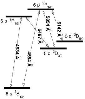
Figure 2: Ba ii simplified atomic model, the Ba iii ionization continuum is taken into account but not shown in the Fig.

Figure 3: Depth-dependence of the branching ratios $\alpha$ (full line), $\beta^{(0)}$ (dotted line) and $\beta^{(2)}$ (dashed line), defined in Eq. (6).

3.2 Partial frequency redistribution effects

In Figs. 4 and 5 we compare the observed intensity and polarization profiles to the results of our non-LTE radiative transfer modeling both with partial frequency redistribution (PFR) and with complete frequency redistribution (CFR). In both cases the magnetic field is set to zero and the standard FALC model of the quiet solar atmosphere is used. In order to fit the observed intensity profiles one has to take into account the effect of macroturbulent velocity fields in the solar atmosphere. This amounts to a smearing of the profiles by a normalized Gaussian function with a width parameter. We assume typical values of the order of 3 km/s for the quadratic mean value of the macroturbulent velocities.

Figure 4: Partial frequency redistribution effects. Intensity profiles for 2 values of the limb distance, d= 4” and 40”. Full lines: observed profiles, dotted lines: calculated profiles with complete frequency redistribution, dashed lines: calculated profiles with partial frequency redistribution.

The intensity profiles, shown in Fig.4, are weakly sensitive to partial frequency redistribution effects (see Uitenbroek & Bruls 1992 for a detailed analysis). We notice that the line width is not well reproduced by our model, the reason is that we have neglected the hyperfine splitting of the lower level of the odd isotopes, which actually broadens the line profile. Fig. 5 shows that the line polarization profiles are strongly affected by partial frequency redistribution effects, both in the line core and in the wings. As expected, we do not reproduce the triple peak structure of the polarization peak either with PFR or with CFR. The computed line polarization is significantly smaller with CFR than with PFR. Complete frequency redistribution leads to zero polarization in the line wings, in contradiction to the observations, whereas the PFR model reproduces quite well the observed polarization profiles in the wings.

Figure 5: Partial frequency redistribution effects. Linear polarization profiles $-Q/I$ for 2 values of the limb distance, d= 4” and 40”. Full lines: observed profiles, dotted lines: profiles calculated with complete frequency redistribution, dashed lines: profiles calculated with partial frequency redistribution.

4 Investigation of the line polarization diagnostic potential

4.1 Sensitivity to temperature variations

The low solar chromosphere is an inhomogeneous medium, with cold and hot components, varying with time (see Avrett 1995, Holzreuter et al. 2006). In order to test the sensitivity of the line to temperature variations we compare the intensity and polarization profiles obtained for two models of the quiet solar atmosphere, i.e. the standard average FALC model and the FALX cold model. As shown in Fig. (6), the intensity profiles obtained for the two models are almost indistinguishable, the reason is probably that non-LTE effects tend to decouple the line source function from the Planck function. However the amplitude of the linear polarization peak, which is related to the anisotropy of the radiation field, shows a higher sensitivity to the atmospheric model. The colder model leads to a slightly smaller value for the maximum of the peak at line center, the effect becomes larger when ones approaches the solar limb and at the limb distance $d=4"$ the linear polarization peak reaches about 1.5% with the FALC model and about 1.3% with FALX. We shall see in the following that these differences do not play a significant role in the diagnosis of microturbulent magnetic fields by means of their Hanle effect in the line.

Figure 6: Intensity and linear polarization profiles for 2 values of the limb distance, d= 4” and 40”. Full lines: observed profiles, dotted lines: profiles calculated with the FALX model, dashed lines: profiles calculated with the FALC model.

4.2 Sensitivity to elastic collisions

The collisional cross-section obtained by Barklem & O’ Mara (BOM) is 3 times larger than the classical Lindholm theory with the Van der Waals approximation; they estimate the relative accuracy of their results at about 10%. We have tested the effect on the line intensity and polarization of varying the elastic collision rate, namely we used the two values $\Gamma_{C}=3.\gamma_{VW}$ (BOM standard result) and $\Gamma_{C}=2.\gamma_{VW}$, where $\gamma_{VW}$ denotes the Van der Waals value. In both cases the calculations were done with PFR and for the FALC model, the results are shown in Fig. (7). We see that there are very few differences between the 2 cases, both in the line intensity and polarization profiles. The line polarization is slightly smaller for the model with the largest collision rate, which is to be expected, but the effect is weak because, as explained previously, the line is formed in a low density medium where radiative broadening dominates over collisional broadening. We notice that in the line wings, which are not sensitive to the Hanle effect, the polarization obtained with the BOM value for the elastic collision rate is in slightly better agreement with the observed profile.

As far as depolarizing collisions are concerned, recently Derouich (2008) has shown that in the low chromosphere, where the $D^{(2)}$ depolarizing collision rate is much smaller than the line radiative transition rate, the depolarization of the ${}^{2}P_{3/2}$ level is mainly due to alignment transfer with the $D_{3/2,5/2}$ metastable levels of Ba ii. The corresponding depolarization increases when the hydrogen density increases, because the alignments of the metastable ${}^{2}D_{3/2,5/2}$ levels are vulnerable to collisions. In order to estimate this effect we solved the statistical equilibrium equations for the five BaII levels shown in Fig. 1 including collisions, radiation and magnetic field effects as in Derouich (2008) i.e. with a single scattering approximation, and we compared with the results of the equivalent two-level model, for 3 values of the hydrogen density. The results are given in the second column of Table 1, where $\Delta p/p_{max}$ is the relative depolarization due to alignment transfer and $p_{max}$ denotes the resonance polarization obtained with an equivalent two-level model. We see that the relative depolarization varies between 30% and 40%.

A physical interpretation of the effect of multi-level coupling on the polarization of the Ba ii D2 line is given here. By solving the statistical equilibrium equations for the five BaII levels shown in Fig. 1 we can estimate the relative importance of the three absorption mechanisms responsible for the atomic polarization of the $P_{3/2}$ upper level. We find that 69% of absorptions take place from the fundamental $S_{1/2}$ level, 3% from the $D_{3/2}$ metastable level and 28% from the $D_{5/2}$ one. The polarisability coefficient of those transitions are $W_{2}=0.5$, 0.32 and 0.02, respectively. The $D_{5/2}\to P_{3/2}$ transition has a low polarisability and it is responsible for an important fraction of the $P_{3/2}$ population. This leads to a decrease of the polarization as compared to the results of the equivalent two-level atom model where the only possible polarizing mechanism is the absorption of radiation from the fundamental level.

Table 1: Depolarizing effect of multi-level alignment transfer on the Ba ii D2 linear polarization and correction factor $f_{c}$ on the magnetic field obtained with an equivalent two-level atom.

$n_{H}$ (cm-3)	${\Delta p\over p_{max}}$	$f_{c}$
0.	0.30	0.60
$3\,10^{13}$	0.35	0.51
$5\,10^{13}$	0.40	0.44

Figure 7: Left panel: Intensity profiles for 2 values of the limb distance, d= 4” and 40”. Right panel: linear polarization for the same values of the limb distance. Full lines: observed profiles, dotted lines: profiles calculated with the standard BOM value for the elastic collision rate $\Gamma_{C}=3.\gamma_{VW}$, dashed lines: profiles calculated for $\Gamma_{C}=2.\gamma_{VW}$.

4.3 Hanle effect

Let us now turn to the Hanle effect in the equivalent two-level atom model. In Fig. (8) we compare the polarization profiles observed at three distances from the solar limb, namely at 4”, 10” and 40”, to those derived from non-LTE radiative transfer modeling with partial frequency redistribution and the Hanle effect, for the atmospheric models FALC and FALX. We first remark that the observations in the line wings, which are not sensitive to the Hanle effect are well recovered in both cases. We recall that the central peak, due to the even isotopes, is sensitive to the Hanle effect of a microturbulent magnetic field, whereas the two secondary peaks, due to the odd isotopes, are not (Belluzzi et al. 2007). We can thus focus on the interpretation of the polarization observed in the central peak, which is modeled here. We see that it is quite well recovered when we introduce the depolarizing Hanle effect of a turbulent magnetic field between 20 Gauss and 30 Gauss. The differences between FALC and FALX results are not meaningful with regard to the accuracy of the polarization measurements.

We now take into account the effect of neglecting alignment transfer with the metastable ${}^{2}D_{3/2,5/2}$ levels. Table 1 gives the correction factor $f_{c}$ that we have to apply to the value of the turbulent magnetic field strength derived from our equivalent two-level model. It is obtained as explained in Derouich (2008) by solving the statistical equilibrium equations for the density matrix elements of the 5-level model of Ba  ii and of the two-level model, in the presence of depolarizing collision, a radiation field and the Hanle effect and comparing the alignment of the ${}^{2}P_{3/2}$ level in both models. The line profiles observed close to the solar limb, are formed at altitudes $z\geq$ 900 km, where the hydrogen density is lower than $5\,10^{13}$ cm^-3 and the correction factor is between 0.60 and 0.51. Let us stress that the correction factor depends in a non-linear way on the magnetic field strength implemented in the density matrix statistical rates; here it was computed for a magnetic field of the order of 15 G. Applying this correction to our previous estimate we find that the turbulent magnetic field strength is between 10 G and 18 G.

Figure 8: Hanle effect of a microturbulent magnetic field. Left panel: observations versus non-LTE modeling for the FALC model, Right panel: observations versus non-LTE modeling for the FALX model. Full lines: observed profiles, at 3 different distances from the solar limb, namely, from top to bottom, 4”, 10” and 40”. Dashed lines: calculated profiles for the same limb distances for B=30 G. Dotted lines: calculated profiles for the same limb distances for B=20 G.

5 Conclusion

The chromosphere is a highly inhomogeneous medium where temperature, velocity and magnetic fields have complex structures that are still poorly investigated. As the magnetic strength decreases with height in the solar atmosphere, the Hanle effect in resonance lines offers a valuable complement to Zeeman diagnostics. We have tested the sensitivity of the linear resonance polarization of the BaII 455.4 nm line to partial frequency redistribution (PFR), temperature variations in the atmospheric model, elastic collisions and weak unresolved magnetic fields. These investigations show that the line polarization is strongly affected by PFR, but that it is weakly sensitive to temperature variations. Recent studies on the depolarizing effects of elastic collisions with hydrogen atoms by Derouich (2008) showed that the line polarization is affected by alignment transfer with the metastable ${}^{2}D$ levels which are not included in the equivalent two-level atom model that we use for modeling the non-LTE polarized line formation. We propose to take this depolarizing mechanism into account by introducing a correction factor on the turbulent magnetic field strength obtained with the equivalent two-level atom model. We estimate this correction factor by solving the statistical equilibrium equations for the density matrix of the 5-levels atomic model including collisions, radiation and magnetic field effects, with a single scattering approximation as in Derouich (2008). This procedure is a first step toward a complete treatment of non-LTE polarized transfer including partial frequency redistribution and full multi-level coupling.

This paper shows that the solar Ba ii D2 line is very well suited for the diagnosis of weak magnetic fields of the order of a few tens of Gauss in the low chromosphere, typically between 900 km and 1300 km above the basis of the photosphere. Our observations are well recovered with a turbulent magnetic field between 10 G and 18 G. These values are significantly lower than those which are derived from the linear limb polarization observed in the SrI line at 406.7 nm or in molecular lines of MgH, which range between 20 G and 50 G (see Faurobert et al 2001, Bommier et al. 2005, Bommier et al. 2006) . But those lines are formed in the upper photosphere, typically between 200 km and 400 km above the basis of the photosphere, where the turbulent magnetic field may very well be stronger than at higher altitudes. We may consider our result as the first quantitative indication of such a decrease of the turbulent magnetic field strength with altitude. Further observations with a better spatial resolution should be performed to measure simultaneously the four Stokes parameters in the BaII line, in order to take advantage of both Hanle and Zeeman effects to obtain a complete view of the magnetic field structure.

- (1) Avrett, E.H. 1995 in Infrared tools for Astrophysics: What’s next?, J.R Kuhn & M.J. Penn eds. (Singapore: World Scientific), 303
- (2) Barklem, P.S. & O’Mara, B.J. 1998, MNRAS, 300, 863
- (3) Belluzzi, L., Trujillo Bueno, J. & Landi Degl’Innocenti, E. 2007, A&A, 666, 588
- (4) Bommier, V. 1997a, A&A, 328, 706
- (5) Bommier, V. 1997b, A&A, 328, 726
- (6) Bommier, V., & Molodij, G. 2002, A&A, 381, 241
- (7) Bommier, V., & Rayrole, J. 2002, A&A, 381, 227
- (8) Bommier, V., Derouich, M., Landi degl’Innocenti, E., Molodij, G., Sahal-Br chot, S. 2005, A&A, 432, 295
- (9) Bommier, V., Landi Degl’Innocenti, E., Molodij, G. 2006, A&A, 458, 625
- (10) Derouich, M., 2008, A&A, 481, 845
- (11) Derouich, M., Sahal-Bréchot, S. & Barklem, P. S. 2004, A&A, 426, 707
- (12) Domke, H. & Hubeny, I. 1988, ApJ, 65, 527
- (13) Faurobert-Scholl, M. 1992, A&A, 258, 521
- (14) Faurobert, M., Arnaud, J., Vigneau, J. & Frisch, H. 2001, A&A, 378, 627
- (15) Fluri, D., & Stenflo, J.O., 1999 A&A, 341, 902
- (16) Fluri, D.M., Nagendra, K.N. & Frisch, H. 2003, A&A, 303
- (17) Fontenla, J. M., Avrett, E. H. & Loeser, R. 1993, ApJ, 406, 319
- (18) Holtzreuter, R., Fluri, D.M. & Stenflo, J.O. 2006, A&A, 449, L41
- (19) Innes, D. E., Lagg, A. & Solanki, S. A. (eds.) 2005, Chromospheric and coronal magnetic fields, ESA SP596
- (20) Malherbe, J. M., Moity, J., Arnaud, J. & Roudier, Th., 2006, A&A, 462, 753
- (21) Rutten, R. J. 1978, Sol. Phys., 56, 237
- (22) Stenflo, J.O., 1994 Solar magnetic fields, Kluwer, Dordrecht, p. 217
- (23) Stenflo, J.O. & Keller, C.U. 1997, A&A, 321, 927
- (24) Uitenbroek, H. & Bruls, J.H.M.J 1992, A&A, 265, 268