Spinor Dynamics of Quantum Accelerator Modes near Higher Order Resonances.

Abstract

Quantum Accelerator Modes were discovered in experiments with Kicked Cold Atoms in the presence of gravity. They were shown to be tightly related to resonances of the Quantum Kicked Rotor. In this paper a spinor formalism is developed for the analysis of Modes associated with resonances of arbitrary order $q\geq 1$. Decoupling of spin variables from orbital ones is achieved by means of an ansatz of the Born-Oppenheimer type, that generates $q$ independent band dynamics. Each of these is described, in classical terms, by a map, and the stable periodic orbits of this map give rise to quantum accelerator modes, which are potentially observable in experiments. The arithmetic organization of such periodic orbits is briefly discussed.

I Introduction.

A kicked system is a Hamiltonian system that is periodically driven by pulses of infinitesimal duration. More than thirty years after the invention of the paradigmatic model of such systems, namely the Kicked Rotor (KR) kr , Kicked Quantum Dynamics is still the focus of active research for a twofold reason. On the one hand, it has given birth to an ever increasing list of variants of the basic original prototypes, which have provided formally simple models for the investigation of quantum-classical correspondence and of some general properties of quantum transport. These include dynamical localization f3 , anomalous diffusion khar2 ; khar1 ; khar3 ; gubo , decay from stable phase-space islands bkm ; bkls ; SFGR05 , electronic conduction in mesoscopic devices fbkkrhb ; okg ; bgr , nondispersive wave packet dynamics dlryb , effects of dissipation on quantum dynamics gabriel , and lately directed transport TM1 ; mont ; dasum . On the other hand, renewed interest on the physical side has been stimulated by experimental realizations raizen1b ; c ; KRexp3 ; phill , which are now possible, under excellent control conditions, thanks to the science and technology of cold and ultra-cold atoms. Unexpected advances of the theory have been prompted by such experiments. For instance, the so-called Quantum Accelerator Modes (QAM) were discovered in experiments with cold atoms in periodically pulsed optical lattices Ox991 ; Ox992 ; Ox995 ; Ox994 . Their underlying theoretical model is a variant of the Kicked Rotor model, the difference being that, in between kicks, atoms are subject to gravity. When the kicking period is close to a half-integer multiple of the Talbot time BB , which is a natural time scale for the system, a fraction of atoms steadily accelerates away from the bulk of the atomic cloud, at a rate and in a direction which depend on various parameter values. Though QAMs are a somewhat particular phenomenon, their theory FGR022 ; FGR021 ; GRF05 ; Rebk is a vast repertory of classic items of classical and quantum mechanics. QAMs are rooted in subtle aspects of the Bloch theory, and have a relation to the Wannier-Stark resonances of Solid-State physics SFGR05 . They are a purely quantal effect, and yet they are explained in terms of trajectories of certain classical dynamical systems, by means of a “pseudo-quasi classical” approximation, where the role of the Planck constant is played by a parameter $\epsilon$, which measures the detuning of the kicking period from a half-integer multiple of the Talbot time. This theory hinges on existence of a “pseudoclassical limit” for $\epsilon\to 0$. That means, for kicking periods close to half-integer multiples of the Talbot time, the quantum dynamics may formally be obtained from quantization of a classical dynamical system, using $\epsilon$ as the Planck constant. This system is totally unrelated from the classical system that is obtained in the proper classical limit $\hbar\to 0$.

Experimental and theoretical investigation on QAMs are currently focused on novel research lines: the observation of QAMs in a Bose-Einstein condensate S ; rafg ; hsgc08 , which allows a precise control on the initial momentum distribution, the analysis of QAMs for special values of the physical parameters lemarie ; shgc08 and, in particular, when the kicking period is close to a rational multiple of Talbot time GS ; GR08 . Theoretical aspects concerning the latter problem are considered in the present paper.

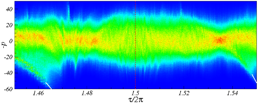
Figure 1: Momentum distributions, in the time dependent gauge, after $t=100$ kicks, for different values of the kicking period near the resonance $\tau_{res}=3\pi$. Red color corresponds to highest probability. The vertical dashed line corresponds to the resonant value. White full lines show the theoretical curves (30), with: (left) $q=2,(r,s)=(1,1)$ and (right) $q=7,(r,s)=(4,1)$ close to the higher order resonance $\tau^{\rm res}/2\pi=p/q=11/7$. The initial quantum distribution is a gaussian wave packet, reproducing the experimental conditions. The other parameters are: $k=1$ and $g=0.0386$. All our numerical simulation refer to the choice $V(\theta)=k\cos\theta$.

QAMS are connected with an important feature of the KR model, namely, the KR resonances IzShep1 , which occur whenever the kicking period is rationally related to the internal frequencies of the free rotor. The dynamics of the rotor at a quantum resonance is invariant under momentum translations by multiples of an integer number. The least positive integer $q$, such that translation invariance in momentum space holds, is the “order” of the resonance (sect. II). The half-Talbot time in atom-optics experiments is the period of the KR resonances of order $q=1$ (i.e. “principal” resonances), so the originally observed QAMs are related to KR resonances of order $1$.

In this paper we consider quantum motion in the vicinity of a higher order KR resonance ($q>1$) in the presence of gravity. Numerical (see fig.1) and heuristic indications GS suggest that higher-order KR resonances, too, may give rise to QAMs. This has been substantiated by a theory GR08 based on a nontrivial reformulation of the original pseudo-classical approximation. It has been remarked that, in the case of higher-order resonances, no pseudoclassical limit exists and similarity to the case of quasi-classical analysis for particles with spin was noted, but not explored. About the latter general problem LF91 ; LF92 , it is known that, although no single well-defined classical limit exists, and so no global quasi-classical phase-space approximation in terms of a unique classical Hamiltonian flow is possible, local quasi-classical approximations are nevertheless still possible, as provided by bundles of trajectories which belong to a number of different Hamiltonian systems.

In this paper we develop a formulation of the problem of QAMs near higher-order resonances in spinor terms. The quantum evolution at exact resonance is described by a multi-component wave function, that is by a spinor of rank $q$, given by the order of the resonance IzShep1 ; CaGua , and is generated by a time-independent spinor Hamiltonian sokzhicas ; SZAC1 . We show that the small-$\epsilon$ analysis of quantum dynamics is formally equivalent to semiclassical approximation for a particle with spin-orbit coupling. Thus QAMs near higher order resonances constitute a particular, though experimentally relevant, model system, in which this crucial theoretical issue can be explored. The semiclassical theory in LF92 is not directly applicable here, because the dynamics is not specified by a self adjoint spinor Hamiltonian, but by a spinor unitary propagator instead. We therefore resort to an “adiabatic” ansatz, which allows decoupling spin dynamics from orbital motion. In this way we obtain $q$ distinct and independent orbital one-period propagators. Each of them may be viewed as the quantization of a formally classical dynamical system, given by a map; however, the “pseudo-Planck constant” $\epsilon$ explicitly appears in such maps, in a form that precludes existence of a $\epsilon\to 0$ limit for the maps themselves, except for the $q=1$ case, in which the pseudo-classical theory of ref. FGR021 ; FGR022 is recovered.
QAMs, detected by numerical simulations of the exact quantum dynamics near higher order resonances, tightly correspond to stable periodic orbits of the maps. The acceleration of the modes is expressed in terms of the winding numbers of the corresponding orbits and of the order of the resonance. Moreover, we derive some theoretical results, which generalize those obtained in FGR021 ; GRF05 for the principal resonances: a formula for the special values of quasi-momenta, which dominate the mode, and a classification of detectable modes by a Farey tree contruction far816 ; HW79 , as a function of the gravity acceleration.

The paper is organized as follows. In sect.II the Floquet operator, describing one-step evolution of a kicked atom in a free-falling frame, is recalled and the resonant spinor dynamics in Kicked Particle (KP) model is briefly reviewed; in sect.III, the quantum motion in the vicinity of a resonance of arbitrary order is related to the problem of a particle with spin-orbit coupling. In sect.IV, a “formally” classical description of the orbital dynamics, associated to the QAMs, is achieved. Finally, in sect.V connections between the theoretical results and possible experimental findings are discussed.

II Background.

II.1 Floquet operator in the “temporal gauge”.

In the laboratory frame, the quantum dynamics of the atoms moving under the joint action of gravity and of the kicking potential, is ruled by the time-dependent Hamiltonian (expressed in dimensionless units):

$$\hat{H}_{L}(t)=\frac{\hat{p}^{2}}{2}-\frac{\eta}{\tau}\hat{x}+kV(\hat{x})\sum_{n=-\infty}^{+\infty}\delta(t-n\tau),$$ (1)

where $\hat{p}$ and $\hat{x}$ are the momentum and position operators. The potential $V(x)$ is a smooth periodic function of spatial period $2\pi$. Denoting $M,T,{\mathrm{K}},{\mathrm{g}}$ and $2\pi/G$ the atomic mass, the temporal period of the kicking, the kicking strength, the gravity acceleration and the spatial period of the kicks, respectively, the momentum, position and mass of the atom in (1) are rescaled in units of $\hbar G$, $G^{-1}$ and $M$. The three dimensionless parameters $k,\tau$ and $\eta$ in (1), which fully characterize the dynamics, are expressed in terms of physical quantities by $k={\mathrm{K}}/\hbar$, $\eta=M{\mathrm{g}}T/(\hbar G)$ and $\tau=\hbar TG^{2}/M=4\pi T/T_{B}$. $T_{B}=4\pi M/(\hbar G^{2})$ is the Talbot time BB and $g=\eta/\tau$ is the rescaled gravity acceleration. Throughout the following $\hbar=1$ is understood.

For $\eta=0$, the Hamiltonian (1) reduces to that of the Kicked Particle model (KP), which is a well-known variant of the Kicked Rotor model (KR), corresponding to the particular choice: $V(x)=k\cos(x)$. The KP differs from the KR because the eigenvalues of particle momentum are continuos while those of the angular momentum of the rotor are discrete. Due to Bloch theorem, the invariance of the KP Hamiltonian, under space translations by $2\pi$, implies conservation of the quasi-momentum $\beta$, which, in the chosen units, is the fractional part of the momentum. The particle momentum is decomposed as $p=N+\beta$ with $N\in{\mathbb{Z}}$ and $0\leq\beta<1$. Conservation of quasi-momentum enables a Bloch-Wannier fibration of the particle dynamics: the particle wave function is obtained by a superposition of Bloch waves, describing the states of independently evolving kicked rotors with different values of the quasi-momentum (called $\beta$-rotors).

A remarkable feature of Hamiltonian (1) is that, unless rescaled gravity $g=\eta/\tau$ assumes exceptional commensurate values, the linear potential term breaks invariance under $2\pi$ space translations. Such an invariance may be recovered by going to a temporal gauge, where momentum is measured w.r.t. free fall. This transformation gets rid of the linear term and the new Hamiltonian reads FGR021 :

$$\hat{H}_{g}(t)=\frac{1}{2}(\hat{N}+\beta+\frac{\eta}{\tau}t)^{2}+kV(\hat{\theta})\sum_{n=-\infty}^{+\infty}\delta(t-n\tau).$$ (2)

where $\theta=x\;{\rm mod}(2\pi)$, $\hat{N}=-id/d\theta$ with periodic boundary conditions.

The quantum motion of a $\beta$-rotor in the “temporal gauge” (that is, “in the falling frame”) is described by the following Floquet operator on $L^{2}({\mathbb{T}})$ ( ${\mathbb{T}}$ denotes the 1-torus, parametrized by $\theta\in[-\pi,\pi[$):

$$\hat{U}_{\beta}(n)=e^{-ikV(\hat{\theta})}e^{-i\frac{\tau}{2}(\hat{N}+\beta+\eta n+\frac{\eta}{2})^{2}}.$$ (3)

where $n\in{\mathbb{Z}}$ denotes the number of kicks. The operator (3) describes evolution from time $t=n\tau$ to time $t=(n+1)\tau$.

II.2 Quantum Resonances.

We consider the problem of Quantum Accelerator Modes in the vicinity of a generic resonance of the $\beta$-rotor. The concept of quantum resonance (QR) is reviewed in this subsection.

A QR occurs whenever quantum evolution commutes with a nontrivial group of momentum translations. A momentum translation $\hat{N}\to\hat{N}+\ell$ (recall $\hbar=1$) with $\ell\in{\mathbb{Z}}$ is described by the operator $\hat{T}^{\ell}=e^{i{\ell}\hat{\theta}}$. In the following we assume $\eta=0$ and then the operator (3) is time-independent. It commutes with $\hat{T}^{\ell}$ if and only if dd : $i)$ $\tau/2\pi=p/q$ with $p,q$ coprime integers; $ii)$ ${\ell}=rq$ with $r\in{\mathbb{N}}$; $iii)$ $\beta=\nu/rp+rq/2$(mod 1), with $\nu\in{\mathbb{Z}}$. In this paper we restrict to “primary” resonances, i.e. to resonances with $r=1$ and $\ell=q$; in this case, $q$ defines the order of the resonance. QR of order 1 are called “principal resonances”.

A theory for QAMs in the vicinity of principal resonances was proposed in FGR022 ; FGR021 . In this paper we consider quantum resonances of arbitrary order $q\geq 1$. The resonant values of the kicking period $(i)$, expressed in physical units, coincide with rational multiples of half of the Talbot time.

We generically denote $\hat{U}_{\mbox{\tiny res}}$ the operator (3) at resonance, and $\beta_{0}$ the resonant values of quasi-momentum, given by the above condition $(iii)$.

II.3 Bloch theory and spinors.

Translation invariance under $\hat{T}^{q}$ enforces conservation of the Bloch phase $\xi\equiv\theta$ mod $2\pi/q$, taking values in the Brillouin zone $\mathbb{B}=[-\pi/q,\pi/q[$. Loosely speaking, this means that $\theta$ only changes by multiples of $2\pi/q$, so $\xi$ has the meaning of “quasi-position”. As we show below, a Bloch-Wannier fibration of the rotor dynamics holds with respect to the quasi-position $\xi$, at a QR.

We use a rescaled quasi-position $\vartheta\equiv q\xi$, and accordingly resize the Brillouin zone to $[-\pi,\pi[$. In all representations where quasi-position is diagonal, the state $|\psi\rangle$ of the rotor is described by a $q$-spinor ${\phi}$, specified by $q$ complex functions $\phi_{l}(\vartheta)=\langle\vartheta,l|\psi\rangle$, $(l=1,\ldots,q)$. We shall use a representation where the spinor $\boldsymbol{\phi}(\vartheta)$, which corresponds to a given rotor wavefunction $\psi(\theta)=\langle\theta|\psi\rangle$, is defined by:

$$\phi_{l}(\vartheta)\;=\;\frac{1}{\sqrt{2\pi}}\;\sum_{m\in{\mathbb{Z}}}\hat{\psi}(l+mq)e^{im\vartheta}\quad\quad\quad l=0,...,q-1.$$ (4)

where $\hat{\psi}(n)$, $n\in{\mathbb{Z}}$ are the Fourier coefficients of $\psi(\theta)$. Equation (4) defines a unitary map $\mathfrak{a}$ of $L^{2}({\mathbb{T}})$ onto $L^{2}({\mathbb{T}})\otimes{\mathbb{C}}^{q}$. Under this map, the (angular) momentum operator $\hat{N}$ is tranformed to:

$$\hat{N}=-i\partial_{\theta}\;\to\;{\mathfrak{a}}(\hat{N}){\mathfrak{a}}^{-1}\;=\;-iq\partial_{\vartheta}\otimes{\bf\hat{I}}+\hat{I}\otimes{\bf\hat{S}},$$ (5)

where $\hat{I}$ and ${\bf\hat{I}}$ are the identity operators in $L^{2}({\mathbb{T}})$ and in ${\mathbb{C}}^{q}$ respectively, and ${\bf\hat{S}}$ is the spin operator in ${\mathbb{C}}^{q}$:

$${\bf\hat{S}}=\sum_{l=0}^{q-1}l|l\rangle\langle l|.\;$$ (6)

where $|l\rangle$, $l=1,\ldots,q-1$ is the canonical basis in ${\mathbb{C}}^{q}$. Thus, in spinor representation, the momentum operator is the sum of the orbital operator $-iq\hat{\partial}_{\vartheta}\otimes{\bf{\hat{I}}}$ and the spin operator $\hat{I}\otimes{\bf{\hat{S}}}$. In this picture, the rotor is characterized by “orbital” observables ($\vartheta$, $-i\partial_{\vartheta}$) and by the spin observable.

Bold symbols denote vectors in ${\mathbb{C}}^{q}$ and matrices.

II.4 Resonant spin dynamics.

At resonance, quasi-position is conserved under the discrete-time evolution defined by (3), so, whenever it has a definite value $\vartheta$, no “orbital” motion occurs, and spin alone changes in time. Therefore the evolution is described by a unitary $q\times q$ matrix ${\bf\hat{A}}(\vartheta)$ such that, as $\psi(\theta)$ evolves into $\hat{U}_{\rm res}\psi(\theta)$, the corresponding spinor $\boldsymbol{\phi}(\vartheta)$ evolves into the spinor ${\bf\hat{A}}(\vartheta)\boldsymbol{\phi}(\vartheta)$. The explicit form of the spin propagator ${\bf\hat{A}}(\vartheta)$ is easily computed by using (3) under resonance conditions. With the specific choice $V(\theta)=\cos(\theta)$, one finds (details can be found in appendix A):

$${\bf\hat{A}}(\vartheta)\;=\;e^{-ik{\bf\hat{V}}(\vartheta)}e^{-i{\bf\hat{G}}},$$ (7)

$${\bf\hat{G}}\;\equiv\;{\bf\hat{G}}_{p,q,{\beta_{0}}}\;=\;\pi\frac{p}{q}({\bf\hat{S}}+{\beta_{0}}{\bf\hat{I}})^{2},$$ (9)

$${\bf\hat{V}}(\vartheta)=\frac{1}{2}\left\{\sum_{l=0}^{q-2}\left(|l\rangle\langle l+1|+|l+1\rangle\langle l|\right)+|0\rangle\langle q-1|e^{i\vartheta}+|q-1\rangle\langle 0|e^{-i\vartheta}\right\}.$$

II.5 Bands.

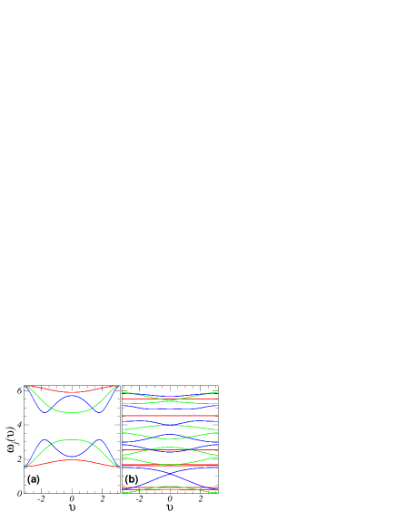
Figure 2: Eigenvalues of the resonant Hamiltonian ${\bf\hat{H}}^{\rm res}(\vartheta)$ for different values of the kicking constant $k=1$ (red), $3$ (green) and $5$ (blue) and (a) $q=2,p=3$, (b) $q=7,p=11$.

The “resonant Hamiltonian” ${\bf\hat{H}}^{\rm res}(\vartheta)$ is a hermitean matrix of rank $q$ such that:

$${\bf\hat{A}}(\vartheta)=e^{-i{\bf\hat{H}}^{\rm res}(\vartheta)}.\\$$ (10)

It is uniquely defined, under the condition that its eigenvalues (i.e., the eigenphases of ${\bf\hat{A}}(\vartheta)$) lie in $[0,2\pi[$. Explicit calculation of eigenvalues and eigenvectors of $\hat{\bf A}(\vartheta)$, hence of the resonant Hamiltonian, is trivial for $q=1$, and is easily performed for $q=2$ in terms of Pauli matrices SZAC1 (such a case is reviewed in appendix B). However, for $q>2$ analytical calculation is prohibitive.
Eigenphases of $\hat{\bf A}(\vartheta)$ are smooth periodic function of quasi-position $\vartheta$. As $\vartheta$ varies in $[-\pi,\pi[$, they sweep bands in the quasi-energy spectrum of the resonant evolution described by $\hat{U}_{\mbox{\tiny res}}$ cs . They also depend on the kicking strength $k$ and will be denoted by $\omega_{l}=\omega_{l}(\vartheta,k)$ in the following ($l=0,...,q-1$). In the case $q=1$, $\omega_{0}(\vartheta,k)=k\cos(\vartheta)$. For $q>1$ the eigenvalues are nontrivial functions of the kick strength $k$. For fixed $q>2$ bandwidths tend to increase with $k$, eventually giving rise to complex patterns of avoided crossings. Examples of $\vartheta$- and $k$-dependence of eigenphases are shown in fig.2 for $q=2$ (a) and $q=7$ (b). For $q>2$ the bandwidths depend also on $l$.

In the resonant representation (i.e. in the representation in which the resonant propagators (10) are diagonal), the spinor components (4) evolve independently.

III Near-resonant dynamics and spin-orbital decoupling.

We are interested in quantum motion, described by (3), in the vicinity of a QR, namely when the kicking period is $\tau=2\pi p/q+\epsilon$, where the detuning $\epsilon$ of the period from the resonant period $\tau_{\rm res}=2\pi p/q$ is assumed to be small. The one-step evolution operator (3) may be factorized as:

$$\hat{U}_{\beta}(n)=\hat{U}_{\rm res}\cdot\hat{U}_{\rm nr}(n)$$ (11)

$$\hat{U}_{\rm nr}(n)=e^{-i\left[\frac{1}{2}\epsilon\hat{N}^{2}+D_{n}\hat{N}\right]},$$ (12)

where $D_{n}=\tau(\beta+\eta n+{\eta}/{2})-2\pi p{\beta_{0}}/q.$

III.1 “Adiabatic” decoupling of spinor and orbital motions.

Translation invariance (in momentum) is now broken by $\hat{U}_{\rm nr}$ , so quasi-position is not conserved any more. The evolution of a spinor ${\phi}\in L^{2}({\mathbb{T}})\otimes{\mathbb{C}}^{q}$ is ruled by the time-dependent Schrödinger equation:

$$i\epsilon\frac{\partial}{\partial t}{\phi}\;=\;\hat{H}(t){\phi}\;,\qquad\qquad\qquad\hat{H}(t)=\epsilon\hat{H}^{\rm res}\cdot\sum_{n=-\infty}^{+\infty}\delta(t-n)+\hat{H}_{0}(t),$$ (13)

$$\hat{H}_{0}(t)=\frac{1}{2}\epsilon^{2}(-iq\partial_{\vartheta}\otimes{\bf\hat{I}}+\hat{I}\otimes{\bf\hat{S}})^{2}+\epsilon D_{[t]}(-iq\partial_{\vartheta}\otimes{\bf\hat{I}}+\hat{I}\otimes{\bf\hat{S}}).$$ (14)

where $[t]$ denotes the integer part of $t$ and $(\hat{H}^{\rm res}\phi)(\vartheta)={\bf\hat{H}}^{\rm res}(\vartheta)\boldsymbol{\phi}(\vartheta)$. Note that $\hat{H}_{0}(t)$ is constant in between kicks.

Both sides of the Schrödinger equation have been multiplied by $\epsilon$, to make it apparent that the detuning $\epsilon$ plays the role of an effective Planck constant in what concerns the motion between the $\delta$-kicks.

The spinor components are mixed by (14) during the evolution; we use an ansatz of Born-Oppenheimer type in order to decouple orbital (slow) motion from spin (fast) motion.

The detuning $\epsilon$ controls as well the separation between the different time scales of the system. At exact resonance (i.e. $\epsilon=0$) the decoupling is exact, because motion is restricted to the eigenspaces of the resonant propagator (10). These subspaces are defined by the spectral decomposition of the resonant Hamiltonian, which we write in the form:

$${\bf\hat{H}}^{\rm res}{(\vartheta)}\;=\;\sum\limits_{j=0}^{q-1}\;\omega_{j}(\vartheta,k)\;\hat{\bf P}_{j}(\vartheta)\;\;\;,\;\;\;\hat{\bf P}_{j}(\vartheta)\;=\;|\boldsymbol{\varphi}_{j}(\vartheta)\rangle\langle\boldsymbol{\varphi}_{j}(\vartheta)|\;,$$ (15)

where $\boldsymbol{\varphi}_{j}(\vartheta)$ is the normalized eigenvector of ${\bf\hat{H}}^{\rm res}{(\vartheta)}$ which corresponds to the eigenvalue $\omega_{j}{(\vartheta,k)}$. For each value of $\vartheta$, the operators $\hat{\bf P}_{j}(\vartheta)$ in (15) are projectors in ${\mathbb{C}}^{q}$. We denote by $\hat{P}_{j}$ the projectors in the full Hilbert space $L^{2}({\mathbb{T}})\otimes{\mathbb{C}}^{q}$, which act on spinors according to $(\hat{P}_{j}{\phi})(\vartheta)=\hat{\bf P}_{j}(\vartheta)\boldsymbol{\phi}(\vartheta)$. The subspaces ${\cal H}_{j}$ whereupon the ${\hat{P}}_{j}$ project are the “band subspaces” and are not invariant for the full Hamiltonian (13). By using the ansatz that “band subspaces” be almost invariant for small $\epsilon$, we next decouple the (assumedly “fast”) spin variables from the orbital (“slow”) ones. We assume that the decoupled evolution inside the band subspaces provides a good description of the exact evolution when $\epsilon$ is small, because the leading error terms are linear in $\epsilon$.

Our approximation consists in replacing the exact dynamics, ruled by the Hamiltonian in (13), (14) by an “adiabatic” evolution, generated by the Hamiltonian:

$$\hat{H}^{\mbox{\tiny diag}}(t)\;=\;\sum\limits_{j=0}^{q-1}\;\hat{P}_{j}\;\hat{H}(t)\;\hat{P}_{j}\;=\;\epsilon\hat{H}^{\rm res}\cdot\sum_{n=-\infty}^{+\infty}\delta(t-n)\;+\;\sum\limits_{j=0}^{q-1}\;\hat{P}_{j}\;\hat{H}_{0}(t)\;\hat{P}_{j}\;.$$ (16)

In the case of time-independent Hamiltonians, such projection on “band subspaces”, aimed at separating fast and slow time scales, is basically a Born-Oppenheimer approximation adth . In the case of kicked dynamics this projection should be performed on the “effective”, time-independent Hamiltonian ${\hat{H}}_{\mbox{\tiny eff}}$, which generates over a unit time the same evolution as does the kicked Hamiltonian. The effective Hamiltonian is not known in closed form, although it can be expressed by a sum of infinite terms, ordered in powers of $\epsilon$ SZAC1 ; danaar . Our ansatz is somehow related to a rough approximation ${\hat{H}}_{\mbox{\tiny eff}}\simeq\epsilon\hat{H}^{\rm res}+{\hat{H}}_{0}$. We assume this is valid in some restricted parameter regimes (see further comments in Sect. IV).

A spinor in ${\cal H}_{j}$ has the form $\psi(\vartheta)\boldsymbol{\varphi}_{j}(\vartheta)$ with $\psi\in L^{2}({\mathbb{T}})$ and may thus be described by a scalar wavefunction $\psi(\vartheta)$ (the amplitude of the spinor on the $j$-th resonant eigenstate). Evolution inside the band subspace ${\cal H}_{j}$ is ruled by the “band Hamiltonian” $\hat{H}_{j}(t)=\hat{P}_{j}\;\hat{H}(t)\;\hat{P}_{j}$ and direct calculation by using (13) shows that band Hamiltonians have the following form:

$${\hat{H}}_{j}(t)\;=\;\;\epsilon\omega_{j}(\vartheta,k)\sum\limits_{t^{\prime}=-\infty}^{+\infty}\delta(t-t^{\prime})\;+\;\hat{H}_{0}^{(j)}(t)\;,$$ (17)

where:

$$\hat{H}^{(j)}_{0}(t)\;=\;-\frac{1}{2}\epsilon^{2}q^{2}\partial_{\vartheta}^{2}-\left(\epsilon^{2}q^{2}\langle\boldsymbol{\varphi}_{j}|{\boldsymbol{\dot{\varphi}}_{j}}\rangle+i\epsilon^{2}qS_{j}+i\epsilon qD_{[t]}\right)\partial_{\vartheta}+\frac{1}{2}\epsilon^{2}\left(S^{{}^{\prime\prime}}_{j}-q^{2}\langle\boldsymbol{\varphi}_{j}|{\boldsymbol{\ddot{\varphi}}_{j}}\rangle-i2qS^{{}^{\prime}}_{l}\right)+$$

$$\qquad\qquad\qquad\qquad+\epsilon D_{[t]}\left(S_{j}-iq\langle\boldsymbol{\varphi}_{j}|{\boldsymbol{\dot{\varphi}}_{j}}\rangle\right),$$ (18)

where dots denote derivatives with respect to $\vartheta$, and

$$S_{j}{(\vartheta)}=\langle\boldsymbol{\varphi}_{j}{(\vartheta)}|{\hat{\bf S}}|\boldsymbol{\varphi}_{j}{(\vartheta)}\rangle\;,\quad S^{{}^{\prime}}_{j}{(\vartheta)}=\langle\boldsymbol{\varphi}_{j}{(\vartheta)}|{\hat{\bf S}}|\boldsymbol{\dot{\varphi}}_{j}{(\vartheta)}\rangle,\quad\quad S^{{}^{\prime\prime}}_{j}{(\vartheta)}=\langle\boldsymbol{\varphi}_{j}{(\vartheta)}|{\hat{\bf S}^{2}}|\boldsymbol{\varphi}_{j}{(\vartheta)}\rangle\;.$$ (19)

III.2 Band Hamiltonians.

We now note that the problem can be formulated as the evolution of a particle in a fictitious magnetic field, which takes into account the average effects of spin degree of freedom on the orbital motion.

We derive a simpler form for the band Hamiltonians (eqs.(III.2)). By the introduction of magnetic vector and scalar potentials, the operator (III.1) may be written in the form:

$$\hat{H}_{j}(t)\;=\;\frac{1}{2}\epsilon^{2}q^{2}\left(-i\partial_{\vartheta}-{\mathcal{A}}_{j}{(\vartheta)}\right)^{2}+\epsilon qD_{[t]}\left(-i\partial_{\vartheta}-{\mathcal{A}}_{j}{(\vartheta)}\right)+\frac{1}{2}\epsilon^{2}{\mathcal{B}}_{j}{(\vartheta)}\;.$$ (20)

The “geometric” vector potential ${\mathcal{A}}_{j}{(\vartheta)}$ and the scalar potential ${\mathcal{B}}_{j}{(\vartheta)}$ are determined by the structure of the resonant eigenvectors $\boldsymbol{\varphi}_{j}(\vartheta)$, via the following relations:

$${\mathcal{A}}_{j}{(\vartheta)}=i\langle\boldsymbol{\varphi}_{j}{(\vartheta)}|{\boldsymbol{\dot{\varphi}}}_{j}{(\vartheta)}\rangle-\frac{1}{q}S_{j}{(\vartheta)}$$ (21)

$${\mathcal{B}}_{j}{(\vartheta)}=S^{{}^{\prime\prime}}_{j}{(\vartheta)}+2q\;\Im S^{{}^{\prime}}_{j}{(\vartheta)}-q^{2}{\mathcal{A}}_{j}^{2}{(\vartheta)}+q^{2}\langle{\boldsymbol{\dot{\varphi}}_{j}}{(\vartheta)}|{\boldsymbol{\dot{\varphi}}}_{j}{(\vartheta)}\rangle.$$ (22)

Reality of such potentials follows from (19) and from the fact that $\langle\boldsymbol{\varphi}_{j}{(\vartheta)}|{\boldsymbol{\dot{\varphi}}}_{j}{(\vartheta)}\rangle$ is purely imaginary thanks to normalization. The vector potential is gauge-dependent; eigenvectors $\boldsymbol{\varphi}_{j}{(\vartheta)}$ are determined up to arbitrary $\vartheta$-dependent phase factors and so operator (20) may be further simplified by a gauge transformation, $\boldsymbol{\varphi}_{j}{(\vartheta)}\to\boldsymbol{\varphi}_{j}{(\vartheta)}e^{i\lambda_{j}{(\vartheta)}}.$ Under such a transformation, ${\mathcal{A}}_{j}{(\vartheta)}$ changes to $\tilde{\mathcal{A}}_{j}{(\vartheta)}={\mathcal{A}}_{j}{(\vartheta)}-\dot{\lambda}_{j}{(\vartheta)}$, and ${\cal B}_{j}{(\vartheta)}$ does not change. The transformation may be chosen so that

$$\tilde{\cal A}_{j}{(\vartheta)}\;=\;\mbox{\rm const.}\;=\;-\gamma_{j,q}\;-\varsigma\;\equiv\alpha_{j}\;,$$ (23)

where:

$$\gamma_{j,q}=\frac{1}{2\pi i}\int_{-\pi}^{\pi}d\vartheta\;\langle\boldsymbol{\varphi}_{j}{(\vartheta)}|{\boldsymbol{\dot{\varphi}}}_{j}{(\vartheta)}\rangle\;\;\;,\;\;\varsigma=\frac{1}{2\pi q}\int_{-\pi}^{\pi}d\vartheta\;S_{j}{(\vartheta)}\;.$$

This immediately follows from (21) and from the requirement, that eigenvectors be single-valued. Note that $2\pi\gamma_{j,q}$ is the geometric (Berry’s) phase berph ; bsimon . We thus assume ${\tilde{\mathcal{A}}}_{j}=\alpha_{j}$: this choice corresponds to the Coulomb gauge.
In conclusion, in the $j$-th band subspace, the band dynamics is described by the following Schrödinger equation:

$$i\epsilon\frac{\partial}{\partial t}\psi(\vartheta,t)\;=\;\hat{H}_{j}(t)\;\psi(\vartheta,t),$$

$$\hat{H}_{j}(t)\;=\;\epsilon\omega_{j}(\vartheta,k)\;\sum_{n=-\infty}^{\infty}\delta(t-n)+\frac{1}{2}\epsilon^{2}q^{2}\left(-i\partial_{\vartheta}-\alpha_{j}\right)^{2}+\frac{1}{2}\epsilon^{2}{\mathcal{B}}_{j}{(\vartheta)}+\epsilon qD_{[t]}\left(-i\partial_{\vartheta}-\alpha_{j}\right)$$ (24)

The multicomponent Schrödinger equation (13), for the $q$-spinor wave function $\phi(\vartheta,t)$, is then reduced to $q$ scalar Schrödinger equations (III.2), each of which determines the independent evolution of a rotor wave function $\psi(\vartheta,t)$.

IV Pseudo-classical description of orbital motion.

We now derive a description of the dynamics of the orbital observables ($\vartheta$, $-i\partial_{\vartheta}$), restricted inside each of the band subspaces ${\cal H}_{j}$, by “formally” classical equations of motion.

We introduce a “pseudo-classical” momentum operator $\hat{I}$, defined as follows:

$$\hat{I}=-i\epsilon\partial_{\vartheta}\;,$$ (25)

which differs from the orbital momentum because of the replacement of the Planck constant ($=1$) by $\epsilon$. If the same role is granted to $\epsilon$ in eqs.(III.2), then, in classical terms, the effective band dynamics in the $j$-th band subspace looks like a rotor dynamics, with angle coordinate $\vartheta$ and conjugate momentum $I$, ruled by the kicked Hamiltonian:

$$H_{j}(\vartheta,I,t)=\epsilon\omega_{j}(\vartheta,k)\sum_{t=-\infty}^{+\infty}\delta(t-t^{\prime})+F_{j}(\vartheta,I,t),$$

$$F_{j}(\vartheta,I,t)=\frac{1}{2}q^{2}I^{2}+D_{[t]}qI-\epsilon q^{2}\alpha_{j}I+\frac{1}{2}\epsilon^{2}{\mathcal{B}}_{j}{(\vartheta)}.$$ (26)

Terms, independent of $I$ and $\vartheta$, have been neglected. This Hamiltonian describes a classical kicked dynamics. By dropping terms beyond first order in $\epsilon$, the map from immediately after the $n$-th kick to immediately after the $(n+1)$-th kick is:

$$\vartheta_{n+1}=\vartheta_{n}+q^{2}I_{n}+2\pi\Omega qn+\varrho\;, \qquad\qquad{\rm mod}\;(2\pi),$$ (27)

$$I_{n+1}=I_{n}-\epsilon\dot{\omega}_{j}(\vartheta_{n+1},k)\;,$$

where $\Omega=\eta\tau/(2\pi)$ and $\varrho=q(-\epsilon q\alpha_{j}+\pi\Omega+\tau\beta-2\pi p\beta_{0}/q)$.

The meaning of the pseudoclassical map (27) as a description of the nearly resonant quantum dynamics will be discussed in section IV.3.

IV.1 Pseudo-classical maps and Quantum Accelerator Modes.

We now describe how quantum accelerator modes appear in the present framework.

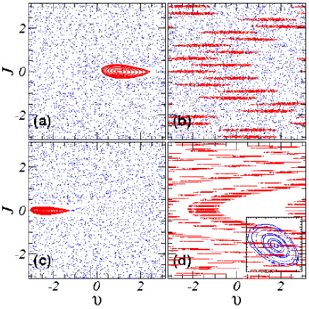
Figure 3: Phase portraits of maps (35) with $k=1$ and $g=0.0386$ and (a) $\tau/2\pi=1.445\;(\epsilon=\tilde{k}=-0.2827),\;\tau\eta=2\pi\Omega=3.2261,(r,s)=(1,1)$, of map (35) with $j=1$; (b) $\tau/2\pi=1.5025\;(\epsilon=\tilde{k}=0.0157),\;\tau\eta=3.4401,(r,s)=(23,21)$, of map (35) with $j=0$; (c) $p/q=11/7,\tau/2\pi=1.5375\;(\epsilon=\tilde{k}=0.2132),\;\tau\eta=3.6023,(r,s)=(4,1)$, of map (28) with $j=3$; (d) $p/q=22/15,\tau/2\pi=1.485\;(\epsilon=\tilde{k}=0.1152),\;\tau\eta=3.3605,r/s=(8,1)$, of map (28) with $j=15$. The periodic orbit has period $r=132$ and it is associated to 132 stability islands; $r$ and $s$ are not coprime ($r=1056$, $s=132$). In the inset a magnification of one of the small islands of the chain is shown.

The explicit dependence on time of map (27) is removed by changing the momentum variable to $J_{n}=q^{2}I_{n}+2\pi\Omega qn+\varrho$. In the variables $(J,\vartheta)$ the map is $2\pi$-periodic in $J$ and so it may be written as a map on the 2-torus:

$$\vartheta_{n+1}=\vartheta_{n}+J_{n} \qquad\qquad{\rm mod}\;(2\pi),$$ (28)

$$J_{n+1}=J_{n}-\epsilon q^{2}\dot{\omega}_{j}(\vartheta,k)+2\pi\Omega q \qquad\qquad{\rm mod}\;(2\pi).$$

In case $q=1$, this map reduces to one which was introduced in FGR022 , in order to explain the QAMs that had been experimentally observed near principal resonances. For $q>1$, it has $q$ different versions, labeled by $l=1,\ldots,q$. Like in the case $q=1$, the stable periodic orbits of each of these versions are expected to give rise to QAMs. Indeed, each stable periodic orbit of map (28) corresponds to a stable accelerating orbit of map (27), because the difference between momentum $I_{n}$ and momentum $J_{n}$ linearly increases with time. More precisely, let $(\vartheta_{0},J_{0})$ be initial conditions for a periodic orbit of period $s$ and winding number $r/s$. The increment of $J$ after time $ns$ (measured in the number of kicks) is $2\pi rn$; therefore, the increment of the original momentum variable is:

$$I_{sn}-I_{0}\;=\;a_{I}sn\;\;\;\;,\;\;\;a_{I}=\frac{2\pi}{q}\left(\frac{r}{qs}-\Omega\right)\;,$$ (29)

with $I_{0}=(J_{0}-\varrho)/q^{2}$. This formula (29) yields the acceleration of a stable orbit of the pseudoclassical dynamics (27), and it is precisely such orbits that may give rise to QAMs in the vicinity of resonances of arbitrary order. As a matter of fact, numerical simulations reveal QAMs near higher order resonances, in correspondence with periodic orbits of maps (28). In sect. V, we explain how the analysis of the stable periodic orbits of maps (28) may help to resolve the complex pattern of QAMs presented in fig.1
Thanks to (5) and (25), the physical momentum $N$ is related to $I$ by $N=qI/\epsilon+j$; therefore, the physical acceleration is given by:

$$a=\frac{2\pi}{\epsilon}\left(\frac{r}{qs}-\Omega\right).$$ (30)

Although the analytical derivation of the maps is based on the resonant Hamiltonian, which is known in closed form only for $q=1,2$, the practical use of (28) only requires the resonant eigenvalues, which can be easily computed by a numerical diagonalization of a $q\times q$ matrix.

In fig.3 examples of phase space of maps (28) are shown for $q=2$ (a,b), $q=7$ (c) and $q=15$ (d), in parameter regimes in which QAMs are present. The plotted periodic orbits correspond to some of the modes shown in fig.1. For instance, in fig.3 (a) the stability island of a fixed point of one of the maps (35) is plotted for $\tau/2\pi=1.455$; this fixed point corresponds to the huge mode on the left side of fig.1. A distribution of phase-space points, which initially fall inside the stability island, describes an ensemble of atoms generating the QAM.

Classical structures, like stability islands, may affect the quantum system only if their size is comparable with the effective Planck constant $\epsilon$. The map (among the $q$ set of eq. (28)), that crucially contributes in determining the observed QAMs, is generally the one with the widest bandwidth.

IV.2 Special values of quasi-momenta.

A QAM arises when the initial wave packet is centered in momentum around $N_{0}$, related to $I_{0}$ by

$$N_{0}=q\frac{I_{0}}{\epsilon}+j=\frac{1}{q\epsilon}(J_{0}+2\pi n)+q\alpha_{j}-\frac{1}{\epsilon}\left(\pi\Omega+\tau\beta-2\pi p{\beta_{0}}/q\right)+j$$ (31)

with $n\in{\mathbb{Z}}$. As in the case for main resonances, we expect that the modes will be especially pronounced when quasimomentum is fine tuned: in view of (31) such optimal values of $\beta$ are determined by the condition:

$$\beta_{\nu}=-\frac{\epsilon}{\tau}(N_{0}-j-q\alpha_{j}+{\beta_{0}})+\frac{J_{0}+2\pi m}{q\tau}-\frac{\eta}{2}+{\beta_{0}}\qquad{\rm mod}\;(1),$$ (32)

with ${\beta_{0}}=\frac{\nu}{p}+\frac{q}{2}$ and $\nu=0,1,..,p-1$. A wave packet initially localized in $N_{0}+\beta_{\nu}$ will be mostly captured inside a QAM; indeed in this case, the overlap between the stability island and the initial wave packet is maximal. Formula (32) is a generalization of the result derived for $q=1$ in FGR022 and experimentally verified in S ; it reduces to the expression in FGR022 for $\alpha_{0}=0$ (see appendix B.1).

This picture is confirmed by fig.4, in which the quantum phase-space evolution of a $\beta$-rotor, with a quasi-momentum given by (32), and the pseudoclassical motion are compared. The initial state of the rotor is a coherent wave packet centered in the $(r,s)=(1,1)$ fixed point, plotted in fig.3(a), corresponding to the $\epsilon$-classical accelerator mode on the left part of fig.1, in the vicinity of $q=2$ resonance. The mode moves with an acceleration equal to 0.2988, according (30).

IV.3 Validity of the Pseudo-Classical Description.

We now come back to the meaning of the pseudo classical description, as “pseudoclassical” dynamics (27) still explicitly retains the “Planck constant” $\epsilon$. In the case when $q=1$, there is a single resonant eigenvalue, given by $\omega_{0}(\vartheta,k)=k\cos(\vartheta)$, so the pseudoclassical dynamics (27) has a well defined limit for $\epsilon\to 0$, $k\to\infty$, $k\epsilon\to\tilde{k}$ with $|\tilde{k}|<\infty$. This limit dynamics was discovered and analyzed in FGR021 ; FGR022 . This is no longer true when $q>1$ and then the relation between the band dynamics and the “pseudoclassical” dynamics (27) is less transparent. The quantum band-dynamics is still, formally, the quantization of the classical kicked dynamics (27) using $\epsilon$ as the Planck constant. Nevertheless, the latter dynamics contains the “Planck constant” $\epsilon$ in crucial ways, which preclude existence of a limit for $\epsilon\to 0$. To see this, note that $\omega_{j}(\vartheta,k)$ depends on its arguments only through the real variables $u=k\sin(\vartheta/q),v=k\cos(\vartheta/q)$ (cf. the form of the resonant evolution (43) in appendix A) that is, $\omega_{j}(\vartheta,k)=G(u,v)$, where $G$ is a smooth oscillatory function, independent of $k$. Hence,

$$\epsilon\dot{\omega}_{j}(\vartheta,k)\;=\;\frac{\epsilon k}{q}\;\left\{\cos(\vartheta/q)\partial_{u}G-\sin(\vartheta/q)\partial_{v}G\right\}$$ (33)

Existence of a limit demands $\epsilon k\to\tilde{k}$; but then, except in the trivial case $\tilde{k}=0$, the arguments of the $G$ functions in (33) diverge and so (33) appears to oscillate faster and faster as $\epsilon\to 0$, without a well-defined limit.
Nonexistence of a pseudoclassical limit for the quantum dynamics was established in GR08 , by a stationary phase approach, with no recourse to the band formalism. It was nonetheless pointed out that, despite absence of such a limit, QAMs may be associated to certain rays, which do correspond to trajectories of some formally classical maps. The meaning of the latter maps is, at most, that of providing local phase space descriptions, near QAMs. Similar remarks apply in the case of the pseudoclassical maps (27).
It is worth recalling that maps (27) were derived from an ansatz, which would be optimally justified if the effective Hamiltonian of kicked dynamics could be replaced by the sum of the free and of the kicking Hamiltonians (sect. III). This approximation is obviously invalid in a global sense, yet, in “spinless” cases, it is known to work remarkably well near stable fixed points SFGR05 ; indeed, in the KR case it yields a pendulum Hamiltonian, which provides a good description of the motion near the stable fixed point of the Standard Map. This may be seen as a qualitative justification for the use of maps (27), if restricted to the search of QAMs.

IV.4 Case $q=2$.

While the expressions in subsect. IV.1 are quite general, we may accomplish a detailed analysis when $q=2$ and $V(\theta)=k\cos(\theta)$. In such a case the eigenvalues $\omega_{j}(\vartheta,k)$ ($j=0,1$) of the resonant Hamiltonian can be written down explicitly (see appendix B):

$$\omega_{j}(\vartheta;k)=-{m_{p}}\left[\frac{\pi}{4}+(-1)^{j}\arccos\left(\frac{\cos(k\cos(\vartheta/2)}{\sqrt{2}}\right)\right],$$ (34)

with ${m_{p}}=(-1)^{\frac{p+1}{2}}$. Therefore, our theory produces two maps (28), which take the form:

$$\vartheta_{t+1}=\vartheta_{t}+J_{t} \quad\quad\quad{\rm mod}\;(2\pi),$$ (35)

$$J_{t+1}=J_{t}+4\pi\Omega-2(-1)^{j}{m_{p}}\tilde{k}\sin\left(\frac{\vartheta_{t+1}}{2}\right)\frac{\sin\left(k\cos\left(\frac{\vartheta_{t+1}}{2}\right)\right)}{\sqrt{1+\sin^{2}\left(k\cos\left(\frac{\vartheta_{t+1}}{2}\right)\right)}} \quad\quad\quad{\rm mod}\;(2\pi).$$

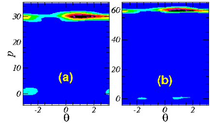
Figure 4: Contour plots at times $t=100$ (a) and $t=200$ (b) of the Husimi distribution of the wave packet of a $\beta$-rotor with $\beta=0.1672$, given by (37) with $j=1$ and $\nu=0$. The rotor is initially prepared in a coherent state centered in the $(r,s)=(1,1)$ fixed point of fig.3(a). The black spots in the centers of the contours are an ensemble of classical phase points, initially distributed in a circle of area $\sim\epsilon$ centered at the mode. They evolve according to the $\epsilon$-classical dynamics (36) with $\varrho=-0.5709$. The other parameter values are $k=1,\tau=1.455*2\pi(\epsilon=-0.2827)$ and $g=0.0386$.

Going back to the time-dependent form the maps are written as

$$\vartheta_{t+1}=\vartheta_{t}+4I_{t}+4\pi\Omega t+\varrho \quad\quad\quad{\rm mod}\;(2\pi),$$ (36)

$$I_{t+1}=I_{t}-(-1)^{j}{m_{p}}\frac{\tilde{k}}{2}\sin\left(\frac{\vartheta_{t+1}}{2}\right)\frac{\sin\left(k\cos\left(\frac{\vartheta_{t+1}}{2}\right)\right)}{\sqrt{1+\sin^{2}\left(k\cos\left(\frac{\vartheta_{t+1}}{2}\right)\right)}} \quad\quad\quad{\rm mod}\;(2\pi),$$

with $\varrho=2\left(\epsilon\delta_{j,1}+\pi\Omega+\tau\beta-\pi p\beta_{0}\right)$ and where we have used $\alpha_{j}=-\frac{1}{2}\delta_{j,1}$ (see appendix B.1).

We remark that in the case $q=2$, avoided crossing between the eigenvalues (34) are absent for an arbitrary value of $k$.

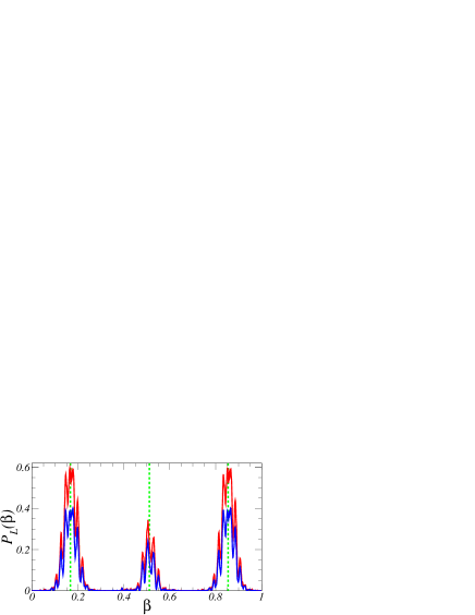
Figure 5: Probability inside a box of extension equal to $L=6\simeq\Delta Jq/|\epsilon|$ in momentum, moving according to (30) for $p=3,q=2,(r,s)=(1,1)$ and $\epsilon=-0.2828$, as a function of quasimomentum $\beta$ of the $\beta$-rotor. $\Delta J$ is the size of the island in $J$. Dashed vertical lines refer to special values of quasimomenta, given by formula (37) with ${\beta_{0}}=\nu/3$, $\nu=0,1,2$, $N_{0}=0,m=0$. The probability is shown at time $t=100$ (red) and $t=200$ (blue). The parameter values are the same as in fig.1.

We may also check the selection criterion for quasimomenta, that in the present case assumes the form:

$$\beta_{j,\nu}=-\frac{\epsilon}{\tau}(N_{0}+{\beta_{0}})+\frac{J_{0}+2\pi n}{q\tau}-\frac{\eta}{2}+{\beta_{0}}\qquad{\rm mod}\;(1),$$ (37)

with $\beta_{0}$ given by $(iii)$ in sect. II and $\nu=0,...,p-1$. A scan over possible $\beta$ values reveals that indeed QAMs are greatly enhanced around the values predicted by (32): this is confirmed by fig.5, in which the momentum probability transferred to the mode is shown as a function of $\beta$.

V Mode spectroscopy and connections with cold atom experiments.

V.1 Farey ordering of QAMs near a fixed resonance.

We now elucidate how our findings apply to inspection of density plots like the one illustrated in fig.1. We point out that such a picture is of direct physical significance, since typical experimental protocols maintain $k$ and $g$ fixed, while performing a scan on the pulse period $\tau$. Such a scan, in the present context, has to be carried out around a resonant value, namely $\tau(\epsilon)=2\pi p/q+\epsilon$. Density plots of momentum distribution disclose the presence of QAMs, since after a fixed number of kicks their momentum is linearly related to the acceleration (30): $a$ depends on $\epsilon$, through the “bare” winding number $q\Omega$

$$q\Omega(\epsilon)=\frac{q}{2\pi}g\left(2\pi\frac{p}{q}+\epsilon\right)^{2}$$ (38)

and on the “dressed” winding number of the pseudo classical map $r/s$, which individuates the mode. We denote by $\Omega^{*}$ the resonant ($\epsilon=0$) value of the “bare” winding number (notice that for $\epsilon=0$ the maps correspond to pure rotation in $J$):

$$\Omega^{*}\equiv q\Omega(0)=2\pi\frac{p^{2}}{q}g,$$ (39)

which is independent of the mapping index $j$. Formula (39) is a generalization of the analogous result found for $q=1$ GRF05 ; all05 .

As analyzed in GRF05 ; all05 for principal resonances, the parameter space of map (28) is characterized by the presence of regions (Arnol’d tongues), in which stable periodic orbits exist. Close to resonances we expect that mode-locking structure of the pseudo classical maps singles out modes whose winding number provide rational approximants to $\Omega^{*}$: at the same time fat tongues are associated to small $s$ values, so the corresponding modes should be more clearly detectable. This is the physical motivation underlying Farey organization of observed modes: whenever we observe two modes labelled by winding numbers $r_{1}/s_{1}$ and $r_{2}/s_{2}$ ($r_{1}/s_{1}<\Omega^{*}<r_{2}/s_{2}$), the fraction with smallest denominator bracketed by the winding pair is the Farey mediant $(r_{1}+r_{2})/(s_{1}+s_{2})$.

We can now analyze in more detail fig.1, which represents a numerical simulation of experimental momentum distribution after $t=100$ vs $\tau$, which assumes values around a second order resonance, namely $\tau^{\rm res}/2\pi=p/q=3/2$. All parameters are chosen to be accessible to experiments and the initial atomic distribution reproduces that employed in Ox991 ; Ox992 ; Ox995 ; Ox994 : $g=0.0386$, $k=1$ and the initial state is a mixture of 100 plane waves sampled from a gaussian distribution of momenta with FWHM $\sim 9$.

Full lines in the figure delineate momentum profiles consistent with the acceleration (30), with $(r,s)$ given by winding number $r/s$ of corresponding stable periodic orbits of maps (28).

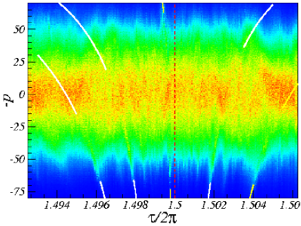
Figure 6: Enlargement of fig.1 in the region $1.49\leq\tau/2\pi\leq 1.50625$, around the resonance $\tau_{res}=3\pi$ $(p/q=3/2)$. Momentum distributions is calculated after $t=200$ kicks. Full lines show the theoretical curves (30): the yellow ones refer to principal convergents of $\Omega^{*}$. Starting from the left, the modes correspond to the stable periodic orbits of maps (35) with: $(r,s)=(14,13),(25,23),(12,11),(23,21)$ and $(11,10)$.

The value of $\Omega^{*}$ and the first few rational approximants (obtained upon successive truncation of the continued fraction expansion), corresponding to detectable modes, are:

$$\Omega^{*}\simeq 1.0913893=1+[10,1,16,3,3,...]$$

$$\frac{r}{s}=1;\;\frac{11}{10};\;\frac{12}{11};...$$ (40)

The first one $(r,s)=(1,1)$ is shown with yellow full line on the left of fig.1 and the stability island of the corresponding fixed point is shown in fig.3 (a). The second and third are marked by full yellow lines in fig.6, which is an enlargement of fig.1 in the region $1.49\leq\tau/2\pi\leq 1.50625$, calculated for time $t=200$. Farey organization is exemplified by the appearance of the $(23,21)$ QAM, whose winding number is the Farey composition of the $(11,10)$ and the $(12,11)$ modes; the correspondent stable periodic orbit is plotted in fig.3(b). Through Farey composition law we may also identify observed modes to the right of $\tau_{res}$, as shown in fig.6.

V.2 Visibility of resonances of different order.

The complexity of mode spectroscopy is further enhanced by the fact that, within some interval in $\tau$, arbitrarily many different resonant values occur. As a matter of fact it is possible to recognize in fig.1 modes coming from a wide set of resonances: besides $q=2$ also $q=7,\,15,\,17,\,21,\,36,\,40$ contribute QAMs in the selected range; this is shown in fig.1 for $q=7$ and in fig.7 for the other resonances. No QAM with $q=13$ could be resolved in the range of fig.1.

Farey composition is still of some use in the identification of the resonances to which modes belong: for instance, the very large mode on the right of the figure belongs to a QR between $p/q=3/2$ and $p/q=2/1$; applying Farey composition successively, we get the sequence $p/q=5/3,8/5$ (outside the plotted range in $\tau$) and then $11/7$, to which the mode belongs. The accumulation point of the resonance $p/q=11/7$ is $\Omega^{*}\simeq 4.1923207=4+[5,...]$. The mode shown in fig.1 corresponds to the first principal convergent of $\Omega^{*}$, i.e. to the fixed point $(r,s)=(4,1)$, shown in fig.3(c). The same occurs for the modes near resonances of higher $q$, shown in fig.6.

We remark that a hierarchy in resonant fractions looks more cumbersome than the one considered for winding numbers, as for instance there does not seem to be any straightforward dependence on the size of $q$. Numerical data however suggest that detectable modes appears in the vicinity of resonances leading to almost integer $\Omega^{*}$, i.e. when the fractional part of $\Omega^{*}$ is closer to the integers 0 or 1 than to their Farey mediant 1/2. In these cases, the resonance may display a mode corresponding to a periodic orbit of period 1. As shown in fig.7, this condition may be fulfilled for different $p/q$ values. Moreover, the absence of observable QAMs with $q=13$ in the range of fig.1, even if $p/q=20/13$ resonance belongs to the plotted $\tau$ range, is consistent with this rough “thumb” rule. Indeed $\Omega^{*}\simeq 7.4624908=7+[2,6,6,..]$, thus its fractional part is closer to 1/2 than to 0.

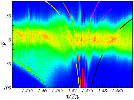
Figure 7: Enlargement of fig.1 in the region $1.45\leq\tau/2\pi\leq 1.49$. The momentum distributions is calculated after $t=200$ kicks. Full lines show the theoretical curves (30); each color refer to a different quantum resonance, namely different values of $p/q$. Starting from the left the modes correspond to: $p/q=3/2$ (theoretical curve not shown), $31/21,59/40,28/19,53/36,25/17$ and $22/15$. These resonances $p_{n}/q_{n}$ lead to almost integer $\Omega^{*}$ and they are exacted from the sequence of Farey fractions obtained starting from $p_{0}/q_{0}=1/1$ and $p_{1}/q_{1}=3/2$: $p_{8}/q_{8}=22/15,\;\Omega^{*}_{8}\simeq 7.82566=8-[5,1,2,1,...],\;(r,s)=(8,1)$ (shown in black); $p_{9}/q_{9}=25/17,\;\Omega^{*}_{9}\simeq 8.9165791=9-[11,1,78,...],\;(r,s)=(9,1)$ (in purple); $p_{10}/q_{10}=28/19;\;\Omega^{*}_{10}\simeq 10.0075=10+[131,...],\;(r,s)=(10,1)$ (in red); $p_{11}/q_{11}=31/21,\;\Omega^{*}_{11}\simeq 11.098678=11+[10,7,2,6,1,...],\;(r,s)=(11,1)$ (in yellow). Further modes are shown in between the mentioned ones: $p/q=53/36=25/17\oplus 28/19$ with $\Omega^{*}\simeq 18.924152=19-[13,5,2,...]$ (shown in pink) and $p/q=59/40=28/19\oplus 31/21$ with $\Omega^{*}\simeq 21.106256=21+[9,2,2,3,...]$ (shown in orange). The $(8,1)$-periodic orbit of the resonance $p_{8}/q_{8}=22/15$ is plotted in fig.3(d).

VI Summary.

The quantum dynamics of quantum accelerator modes, experimentally observed by exposing cold atoms to periodic kicks in the direction of the gravitational field, is theoretically described in terms of spinors, when the pulse period is close to a rational multiple of a characteristic time of the atoms (Talbot time). The reference model is a non-trivial variant of the well-known Kicked Rotator in an almost-resonant regime. If the detuning of the kicking period to the resonant value is assigned the role of the Planck constant, the problem is shown to share similarities with the semiclassical limit of the particle dynamics in presence of spin-orbital coupling. The separation of the spinor and orbital degrees of freedom, is based on an “adiabatic” assumption of Born-Oppenheimer type, valid for small detunings and for values of the parameters in which the QAMs manifest. In these parameter regimes, a description of some properties of the “slow” orbital motion, by means of formally classical equations, is finally achieved. Some results of a previously formulated “pseudo-classical” theory FGR021 , restricted to QAMs near principal resonances, are extended to arbitrary higher order resonances. Potential applications to current experiments on cold atomic gases are proposed.

L.R. acknowledges useful discussions with Shmuel Fishman.

Appendix A Spinor dynamics at exact resonance and without gravity.

The Floquet operator at exact resonance in absence of gravity $\eta=0$ is given by (cp. (3)) :

$$\hat{U}_{\rm res}=e^{-ikV(\hat{\theta})}\cdot e^{-i\pi\frac{p}{q}(\hat{N}+{\beta_{0}})^{2}},$$ (41)

where ${\beta_{0}}=\nu/rp+rq/2$ with $\nu\in{\mathbb{Z}}$. The evolution of spinor components $\phi_{j}{(\vartheta)}$ under $\hat{U}_{\rm res}$ is given by cs :

$$\bar{\phi}_{j}(\vartheta)=\sum_{l=0}^{q-1}(e^{-ik\hat{V}})_{j-l}\;e^{-i\pi\frac{p}{q}(l+{\beta_{0}})^{2}}{\phi}_{l}(\vartheta)$$ (42)

$$(e^{-ik\hat{V}})_{j-l}=\langle j|e^{-i\frac{\vartheta}{q}\hat{\bf S}}{\bf\hat{F}}e^{-ik\hat{V}(\theta)}{\bf\hat{F}}^{\dagger}e^{i\frac{\vartheta}{q}\hat{\bf S}}|l\rangle=\frac{e^{-i(j-l)\frac{\vartheta}{q}}}{q}\sum_{m=0}^{q-1}e^{-i\frac{2\pi}{q}m(j-l)}e^{-ik{\hat{V}}\left(\frac{\vartheta}{q}+\frac{2\pi}{q}m\right)}.$$ (43)

${\bf\hat{F}}$ is the Fourier transform in ${\mathbb{C}}^{q}$: $\langle j|{\bf\hat{F}}|l\rangle=e^{-i\frac{2\pi}{q}jl}/\sqrt{q}$ and $\hat{\bf S}$ is the spin operator (6). Hence from (42), the resonant Floquet operator is decomposable in spin propagators ${\bf\hat{A}}{(\vartheta)}$, given by unitary matrices of rank $q$; namely it acts as $(\hat{U}_{\rm res}{\phi}){(\vartheta)}={{\bf\hat{A}}}{(\vartheta)}\boldsymbol{\phi}{(\vartheta)}$.

Appendix B Case $q=2$: resonant eigenvalues and eigenvectors.

At primary 2nd order ($q=2$) resonances, the resonant values of quasimomentum are $\beta_{0}=\nu/p$ with $\nu=0,1,..,p-1$. We choose $\beta_{0}=0$. From (9) and (9), denoting $v(\vartheta;k)=k\cos(\vartheta/2)$ and ${m_{p}}=(-1)^{\frac{p+1}{2}}$, we find

$${\bf\hat{A}}_{k,p,2,0}=\left(\begin{array}[]{cc}\cos(v(\vartheta;k))&{m_{p}}e^{i\frac{\vartheta}{2}}\sin(v(\vartheta;k))\\ -ie^{-i\frac{\vartheta}{2}}\sin(v(\vartheta;k))&i{m_{p}}\cos(v(\vartheta;k))\end{array}\right).$$ (44)

Matrix (44) can be written in terms of Pauli matrices as follows:

$${\bf\hat{A}}_{k,p,2,0} = e^{i{m_{p}}\frac{\pi}{4}}\left(\cos(\bar{\omega}(\vartheta;k))+i\;\vec{\boldsymbol{x}}(\vartheta;k)\cdot\vec{\boldsymbol{\sigma}}\right),$$ (45)

$$= e^{i{m_{p}}\frac{\pi}{4}}\left(\cos(\bar{\omega}(\vartheta;k))+i\sin(\bar{\omega}(\vartheta;k))\;(\vec{\boldsymbol{n}}(\vartheta;k)\cdot\vec{\boldsymbol{\sigma})}\right),$$ (47)

$$\bar{\omega}(\vartheta;k)=\arccos\left(\frac{\cos(k\cos(\vartheta/2))}{\sqrt{2}}\right),$$

where the vector ${\boldsymbol{x}}(\vartheta;k)\in{\mathbb{R}}^{3}$ has components:

$$x_{1}(\vartheta;k)={m_{p}}\sin\left(\frac{\vartheta}{2}-{m_{p}}\frac{\pi}{4}\right)\sin(v(\vartheta;k)),$$

$$x_{2}(\vartheta;k)=\sin\left(\frac{\vartheta}{2}+{m_{p}}\frac{\pi}{4}\right)\sin(v(\vartheta;k)),$$

$$x_{3}(\vartheta;k)=-\frac{{m_{p}}}{\sqrt{2}}\cos(v(\vartheta;k));$$ (48)

$\vec{\boldsymbol{n}}=\vec{\boldsymbol{x}}/x$ is a unit vector in ${\mathbb{R}}^{3}$, and $x(\vartheta;k)=||{\boldsymbol{x}}(\vartheta;k)||$.

Using a well-known formula, equation (45) may be written:

$${\bf\hat{A}}_{k,p,2,0}=e^{i{m_{p}}\frac{\pi}{4}}e^{i\bar{\omega}(\vartheta;k)\;\vec{\boldsymbol{n}}(\vartheta;k)\cdot\vec{\boldsymbol{\sigma}}},$$ (49)

which directly yields to the Resonant Hamitonian for this case:

$${\bf\hat{H}}^{\rm res}_{k,p,2,0}=-\left[{m_{p}}\frac{\pi}{4}+\bar{\omega}(\vartheta;k)\;\vec{\boldsymbol{n}}(\vartheta;k)\cdot\vec{\boldsymbol{\sigma}}\right].$$ (50)

As matrix $\vec{\boldsymbol{n}}\cdot\vec{\boldsymbol{\sigma}}$ has eigenvalues $\pm 1$, the eigenvalues of the resonant fiber are:

$$\lambda^{(j)}(\vartheta,k)=e^{i{m_{p}}\left[\frac{\pi}{4}+(-1)^{j}\bar{\omega}(\vartheta;k)\right]}=e^{-i\omega_{j}(\vartheta;k)}$$ (51)

$$\omega_{j}(\vartheta;k)=-{m_{p}}\left[\frac{\pi}{4}+(-1)^{j}\bar{\omega}(\vartheta;k)\right]\qquad\qquad j=0,1.$$ (52)

Normalized eigenvectors are:

$${\boldsymbol{\varphi}}_{j}(0,\vartheta)=e^{i\gamma_{j}(\vartheta)}\frac{\sin(v(\vartheta;k))}{\sqrt{a_{j}(\vartheta;k)}};$$ (53)

$${\boldsymbol{\varphi}}_{j}(1,\vartheta)=e^{i\gamma_{j}(\vartheta)}e^{-i\frac{\vartheta}{2}}\frac{i-{m_{p}}}{2}\frac{b_{j}(\vartheta;k)}{\sqrt{a_{j}(\vartheta;k)}};$$ (54)

$$a_{j}(\vartheta;k)=1+\sin^{2}(v(\vartheta;k))+(-1)^{j}\cos(v(\vartheta;k))\sqrt{1+\sin^{2}(v(\vartheta;k))},$$ (55)

$$b_{j}(\vartheta;k)=\cos(v(\vartheta;k))+(-1)^{j}\sqrt{1+\sin^{2}(v(\vartheta;k))}.$$ (56)

The $\gamma_{j}(\vartheta)$ are arbitrary phases. For $n_{0}\pi\leq k<(n_{0}+1)\pi$ ($n_{0}\in{\mathbb{N}}$), $a_{1}(\vartheta;k)$ has a finite set of zeros in $\{\vartheta_{n}=\pm 2\arccos(\pi n/k),0\leq n\leq n_{0}\}$. Discontinuities in the zeros of $a_{1}(\vartheta;k)$ may be removed by appropriate choices of $\gamma_{1}$. For $k<\pi$ and $-\pi<\vartheta\leq\pi$, one may choose, e.g. $\gamma_{j}(\vartheta)=\frac{\vartheta}{2}\delta_{j,1}$.

For increasing values of the kicking strength $k$, eigenvalues (52) display thicker and thicker oscillations. An example is shown in fig.2 (a), for $k=1,3,5$. Nevertheless, contrary to higher values of $q$, in case $q=2$, the two eigenvalues (52) neither cross nor become closer that a minimal gap, equal to $\pi/2$, for arbitrary high values of $k$. As a matter of fact, the band width of each eigenvalue, defined as $B_{j}(k)=|\bar{\omega}(\vartheta_{max};k)-\bar{\omega}(\vartheta_{min};k)|$, with $\vartheta_{max}$ and $\vartheta_{min}$ absolute maximum and minimum points in $[0,2\pi[$, does not exceed $\pi/2$. For $k<\pi$, $B_{j}(k)$ is an increasing function of $k$ equal to $B_{j}(k)=|\bar{\omega}(0;k)-\bar{\omega}(\pi;k)|=|\arccos(\cos(k\cos(\vartheta/2)/\sqrt{2}))-\pi/4|$; for $k>\pi$, $B_{j}(k)=|\bar{\omega}(\vartheta_{1};k)-\bar{\omega}(\pi;k)|=\pi/2$.

For $\beta_{0}=\nu/p$, the same results hold, apart for a constant phase factor in (44) and $m_{p}$ replaced by $-m_{p}$ for $\nu$ odd.

B.1 Vector and Scalar potential.

The vector and scalar potentials can be explicitly computed, using analytical expressions of the eigenvectors of resonant fiber (and choosing phases $\gamma_{j}(\vartheta)=\frac{\vartheta}{2}\delta_{j,1}$). First one computes:

$$S_{jj}{(\vartheta)}=\sum_{l=0}^{1}l|\langle l|\boldsymbol{\varphi}_{j}{(\vartheta)}\rangle|^{2}=\frac{1}{2}\frac{(b_{j})^{2}}{a_{j}},$$

$$S^{{}^{\prime\prime}}_{jj}{(\vartheta)}=\sum_{l=0}^{1}l^{2}|\langle l|\boldsymbol{\varphi}_{j}{(\vartheta)}\rangle|^{2}=S_{jj},$$

$$S^{{}^{\prime}}_{jj}{(\vartheta)}=\sum_{l=0}^{1}l\langle\boldsymbol{\varphi}_{j}{(\vartheta)}|l\rangle\langle l|\boldsymbol{\dot{\varphi}}_{j}{(\vartheta)}\rangle=\frac{1}{2a_{j}}\left(b_{j}\dot{b}_{j}-\frac{1}{2a_{j}}\dot{a_{j}}(b_{j})^{2}+\frac{i}{2}(b_{j})^{2}(\delta_{j,1}-1)\right),$$

$$i\langle\boldsymbol{\varphi}_{j}{(\vartheta)}|\boldsymbol{\dot{\varphi}}_{j}{(\vartheta)}\rangle=-\dot{\gamma}_{j}{(\vartheta)}+\frac{1}{4}\frac{(b_{j})^{2}}{a_{j}},$$

$$\langle\boldsymbol{\dot{\varphi}}_{j}{(\vartheta)}|\boldsymbol{\dot{\varphi}}_{j}{(\vartheta)}\rangle=\frac{1}{a_{j}}\left((\dot{v})^{2}\cos^{2}v+\frac{1}{2}(\dot{b}_{j})^{2}+\frac{1}{8}({b}_{j})^{2}-\frac{1}{4}\frac{(\dot{a}_{j})^{2}}{{a}_{j}}\right)+\frac{1}{4}\delta_{j,1}\left(1-\frac{({b}_{j})^{2}}{{a}_{j}}\right),$$

and then the vector and scalar potentials are given by:

$${\mathcal{A}}_{j}{(\vartheta)}\equiv\alpha_{j}=-\frac{1}{2}\delta_{j,1},$$ (57)

$${\mathcal{B}}_{j}{(\vartheta)}=\frac{4}{a_{j}}\left((\dot{v})^{2}\cos^{2}v+\frac{1}{2}(\dot{b}_{j})^{2}-\frac{1}{4}\frac{(\dot{a}_{j})^{2}}{{a}_{j}}\right)=\frac{2(\dot{v})^{2}}{(1+\sin^{2}v)^{2}},$$ (58)

with $v\equiv v(\vartheta,k)=k\cos(\vartheta/2)$.

For $q=1$ the resonant fiber is a matrix with a single element $\exp(-iv(\vartheta,k))$, with eigenfunction $\varphi_{0}{(\vartheta)}=\exp(in\vartheta)/\sqrt{2\pi}$ ($n\in{\mathbb{Z}}$); $S_{00}=0$ and therefore (21) it yields ${\mathcal{A}}_{0}{(\vartheta)}\equiv\alpha_{0}=-n$ with $n\in{\mathbb{Z}}$ and ${\mathcal{B}}_{0}{(\vartheta)}=0$.

References

- (1) G. Casati, B. V. Chirikov, F. M. Izrailev, and J. Ford, in Lectures Notes in Physics , edited by G. Casati and J. Ford (Springer, Berlin, 1979), Vol. 93.
- (2) F.M.Izrailev, Phys. Rep. 196, 299, (1990); S. Fishman, in Proceedings of the International School of Physics Enrico Fermi; Varenna Course CXIX, G.Casati, I.Guarneri and U. Smilansky eds. (North-Holland 1993).
- (3) R. Lima and D. Shepelyansky, Phys. Rev. Lett. 67, 1377, (1991).
- (4) T. Geisel, R. Ketzmerick, and G. Petschel, Phys. Rev. Lett. 67, 3635, (1991).
- (5) R. Artuso, F. Borgonovi, I. Guarneri, L. Rebuzzini and G. Casati, Phys. Rev. Lett. 69, 3302, (1992).
- (6) I. Guarneri and F. Borgonovi, J.Phys. A Math. Gen. 26, 119, (1993).
- (7) A. Backer, R.Ketzmerick, and A. Monastra, Phys. Rev. Lett. 94, 054102, (2005).
- (8) A. Backer, R.Ketzmerick, S. Lock and L.Schilling, Phys. Rev. Lett. 100, 104101, (2008).
- (9) M. Sheinman, S. Fishman, I. Guarneri, L. Rebuzzini, Phys. Rev. A 73, 052110, (2006).
- (10) J. Feist, A. Bäcker, R. Ketzmerick, S. Rotter, B. Huckestein, and J. Burgdo, Phys. Rev. Lett. 97, 116804, (2006).
- (11) A. Ossipov, T. Kottos, and T. Geisel, Europhys. Lett. 62 (5), 719, (2003).
- (12) F. Borgonovi, I. Guarneri, and L. Rebuzzini, Phys. Rev. Lett. 72, 1463, (1994).
- (13) F.B. Dunning, J. C. Lancaster, C. O. Reinhold, S. Yoshida and J. Burgdorfer, Adv. At. Mol. Opt. Phys 52, 49, (2005).
- (14) G.G. Carlo, G. Benenti and D.L. Shepelyansky, Phys. Rev. Lett. 95, 164101, (2005).
- (15) H. Schanz, M.F. Otto, R. Ketzmerick, and T. Dittrich, Phys. Rev. Lett. 87, 070601, (2001).
- (16) C. E. Creffield, G. Hur, and T. S. Monteiro, Phys. Rev. Lett. 96, 024103, (2006).
- (17) I. Dana, V. Ramareddy, I. Talukdar,and G. S. Summy, Phys. Rev. Lett. 100, 024103, (2008).
- (18) F.L. Moore, J.C. Robinson, C.F. Bharucha, B. Sundaram, and M.G. Raizen, Phys.Rev.Lett. 75, 4598, (1995).
- (19) H. Amman, R. Gray, I. Shvarchuck, N. Christensen, Phys. Rev. Lett. 80, 4111, (1998),
- (20) P. Szriftgiser, J. Ringot, D. Delande, J.C. Garreau, Phys. Rev. Lett. 89, 224101, (2002).
- (21) C. Ryu, M.F. Andersen, A. Vaziri, M.B. d’Arcy, J.M. Grossmann, K. Helmerson, W.D. Phillips, Phys. Rev. Lett. 96, 1604031, (2006).
- (22) M.K. Oberthaler, R.M. Godun, M.B. d’Arcy, G.S. Summy and K. Burnett, Phys.Rev.Lett. 83, 4447, (1999).
- (23) R.M. Godun, M.B. d’Arcy, M.K. Oberthaler, G.S. Summy, and K. Burnett, Phys. Rev. A 62, 013411, (2000).
- (24) S. Schlunk, M.B. d’Arcy, S.A. Gardiner, G.S. Summy, Phys. Rev. Lett. 90, 124102, (2003).
- (25) M. B. d’Arcy, R.M. Godun, D. Cassettari, and G. S. Summy, Phys. Rev. A 67, 023605, (2003).
- (26) M.V.Berry and E.Bodenschatz, J. Mod. Opt. 46, 349, (1999).
- (27) S. Fishman, I. Guarneri, and L.Rebuzzini, Phys. Rev. Lett. 89, 084101, (2002).
- (28) S. Fishman, I. Guarneri, and L.Rebuzzini, J. Stat. Phys. 110, 911, (2003).
- (29) I. Guarneri, S. Fishman, and L. Rebuzzini, Nonlinearity 19, 1141, (2006).
- (30) R. Hihinashvili, T. Oliker, Y.S. Avizrats, A. Jomin, S. Fishman, and I. Guarneri , Physica D 226, 1, (2007).
- (31) G. Behinaein, V. Ramareddy, P. Ahmadi, and G. S. Summy, Phys. Rev. Lett 97, 244101, (2006).
- (32) L. Rebuzzini, R. Artuso, S. Fishman, and Italo Guarneri, Phys. Rev. A 76, 031603(R), (2007).
- (33) P. L. Halkyard, M. Saunders, S. A. Gardiner, and K. J. Challis, arXiv:0807.2587, (2008).
- (34) G. Lemarie and K. Burnett, arXiv:quant-ph/0602204, (2006).
- (35) M. Saunders, P. L. Halkyard, S. A. Gardiner and K. J. Challis, arXiv:0806.3894, (2008).
- (36) I.Guarneri and L. Rebuzzini, Phys. Rev. Lett. 100, 234103, (2008).
- (37) G. Summy, private communication.
- (38) F.M. Izrailev and D.L. Shepelyansky, Theor. Mat. Phys. 43, 353, (1980).
- (39) R.G. Littlejohn and W.G. Flynn, Phys. Rev. A 44, 5239, (1991).
- (40) R.G. Littlejohn and W.G. Flynn, Phys. Rev. A 45, 7697, (1992).
- (41) G. Casati and I. Guarneri, Comm. Math. Phys. 95 , 121, (1984).
- (42) V.V. Sokolov, O.V. Zhirov, D. Alonso, and G. Casati, Phys. Rev. Lett. 84, 3566, (2000).
- (43) V.V. Sokolov, O.V. Zhirov, D. Alonso, and G. Casati, Phys. Rev. E 61, 5057, (2000).
- (44) J. Farey, Philos. Mag. 47, 385, (1816).
- (45) G.H. Hardy and E. M. Wright, An Introduction to the Theory of Numbers, (Clarendon, Oxford, 1979).
- (46) I. Dana and D.L. Dorofeev, Phys. Rev. E, 73, 026206, (2006).
- (47) S.J. Chang and K.J Shi, Phys. Rev. A 34, 7, (1986).
- (48) S. Teufel, Adiabatic Perturbation Theory in Quantum Dynamics, Lecture Notes in Mathematics 1821, Springer Berlin/Heidelberg, (2003).
- (49) I. Dana, E. Eisenberg, and H. Shnerb, Phys. Rev. Lett. 74, 686, (1995).
- (50) M.V. Berry, Proc. R. Soc. A 392, 45, (1984).
- (51) B. Simon, Phys. Rev. Lett. 51, 2167, (1983).
- (52) A. Buchleitner, M.B. d’Arcy, S. Fishman, S.A. Gardiner, I. Guarneri, Z.Y. Ma, L. Rebuzzini, G.S. Summy, Phys. Rev. Lett. 96, 164101, (2006).