Manifestation of three-body forces in three-body Bethe–Salpeter and light-front equations

Abstract

Bethe–Salpeter and light-front bound state equations for three scalar particles interacting by scalar exchange-bosons are solved in ladder truncation. In contrast to two-body systems, the three-body binding energies obtained in these two approaches differ significantly from each other: the ladder kernel in light-front dynamics underbinds by approximately a factor of two compared to the ladder Bethe–Salpeter equation. By taking into account three-body forces in the light-front approach, generated by two exchange-bosons in flight, we find that most of this difference disappears; for small exchange masses, the obtained binding energies coincide with each other.

1 Introduction

Relativistic two-body systems are often treated using the ladder truncation in the Bethe–Salpeter (BS) framework [1] or in light-front dynamics (LFD) [2, 3]. These two approaches give results very close to each other for the binding energy [4] and also for electromagnetic form factors [5] in the spinless case. Binding energies of a two-fermion system were calculated both in the BS approach in [6] and in LFD [7] and again the results turned out to be rather close to each other.

In these cases, the relativistic calculations using either the BS approach or LFD lead to binding energies that are quite different from the non-relativistic binding energy, obtained by solving the Schrödinger equation. The relativistic effects are more important for larger binding energy. In addition, they are also important for small binding energy, if the mass of the exchange particle is large enough, that is, of the order of the constituent mass [4].

Here we extend the same methods, the BS approach and LFD, to scalar three-body bound states, using a one-boson exchange kernel. Eventually, the goal is to extend these methods to bound states of fermions: e.g. using a meson-exchange model in the case of 3-nucleon bound states (triton, ³He), and baryons as bound states of three (non-perturbatively dressed) quarks interacting via gluons. For simplicity however, and as a first step, we restrict ourselves here to spinless systems. Preliminary results for the three-body BS equation with a one-boson exchange kernel have been presented in [8]. As far as we know, the LFD three-body bound state equations with one-boson exchange kernel has never been solved for such systems. Previously, the LFD equation was solved in [9, 10] for zero-range interaction. Its solution was also found in the relativistic quantum-mechanical approach for scattering states [11], with a phenomenological mass operator.

It is important to note that the actual ladder kernels in the BS approach and in LFD are not identical, nor are they given by the same graphs. In the BS ladder kernel, there is no notion of time-ordering in the diagrams. On the other hand, the kernel for the LFD equation is given by the time-ordered graphs in the light-front (LF) time.

Figure 1: (a) Top: Feynman ladder graph with two exchanges. (b) Bottom: One of six time-ordered graphs, generated by the ladder Feynman graph (a).

Thus, the second iteration in the two-body ladder BS equation (the second-order Feynman box graph, Fig. 1(a)), when represented as a set of time-ordered graphs, turns into six LF time-ordered graphs, including two so-called “stretched boxes” with two exchange particles in the intermediate state. One of such stretched boxes is shown in Fig. 1(b). These stretched boxes with two (and more) exchange particles in the intermediate state are implicitly included in the BS equation, but they are not generated by iteration of the LF ladder kernel; therefore, they are omitted in the corresponding LFD bound state equation. In principle, this will cause a difference between the BS and LFD results. However, direct examination of the stretched boxes [12] shows that they are small. Being explicitly included in the LF kernel, they result in a small correction to the binding energy [13]. This explains, why the BS and LFD two-body binding energies are very close to each other, despite the fact that the kernels are not identical.

In the three-body problem, the situation is quite different: even with a simple one-boson exchange kernel, new interesting and important features emerge, highlighting differences between the BS approach and LFD. To be specific, in a three-body problem the difference between LFD and time-ordered iterated BS kernels cannot be reduced to stretched boxes: new LFD diagrams appear, which are shown in Fig. 2.

     

     

     

     

Figure 2: Contribution in three-body forces from the two exchange-bosons in flight ($K^{(1-8)}_{123}$) and from pair-creation ($K^{(9)}_{123}$).

Like stretched boxes, these diagrams cannot be constructed by iterations of the two-body LF kernel. In contrast to the stretched boxes, they do not contain any loops. These graphs generate three-body forces which are not taken into account in the three-body LFD equation with ladder kernel. On the other hand, they are implicitly included in the three-body BS equation.

Three-body nucleon forces have been discussed for several decades. In recent years, there has been an increased interest in 3-nucleon forces due to high precision few-body calculations. The need for three-body forces results from nuclear phenomenology (see for review Ref. [14]). In particular, three-body forces remove the underbinding of light nuclei found with local two-body forces. With nonlocal two-body potentials there seems to be less of a need for three-body forces from a phenomenological point of view [15]. The diagrams depicted in Fig. 2 represent a part of three-body forces for nucleons. Another part arises due to excitation of intermediate isobars (most notably $\Delta$-excitations). The first-order relativistic corrections due to the first eight graphs of Fig. 2, was first found in Ref. [16]. Its contribution to the triton binding energy was calculated in Ref. [17]. In Ref. [18] it was shown that this relativistic correction cancels with the corresponding relativistic correction to the second iteration of the one-boson exchange. Due to this cancellation, the sum of these two corrections does not contribute in the Schrödinger equation. However, in a truly relativistic framework, the full graphs Fig. 2 (not a first-order relativistic correction) should be taken into account.

Both the BS approach and LFD provide us with a relativistic framework to study relativistic three-body bound states. With modern computer resources, we can now solve these bound state equations in ladder truncation without further approximations (at least for spinless systems). These calculations serve as a theoretical laboratory where we can study the importance of three-body forces of relativistic origin, like the ones generated by the diagrams in Fig. 2. By contrasting results from the BS approach and LFD we can elucidate their contribution (if any) to the binding energy. Note that in the scalar model under consideration here, we have no analog of the three-body forces originating from isobar excitations, so we cannot asses the relative importance of three-body forces due to isobar excitations; nor do we have any means to asses the role of intrinsic three-body forces such as $NNN\to NNN$ point interactions, or, in QCD, three-body forces due to the triple gluon vertex.

The aim of this paper is two-fold: (i) First of all, we will solve, for the first time, the three-body bound state BS and LFD equations with a one-boson exchange kernel and compare the corresponding binding energies. We shall see that, in contrast to the two-body case, the binding energies found in these two approaches do not coincide with each. The LFD binding energy is significantly smaller than the BS binding energy (i.e. the LF ladder kernel underbinds compared to the BS ladder kernel). (ii) Then, in order to identify explicitly the origin of this difference, we calculate perturbatively the contribution to the LFD binding energy from the three-body forces depicted in Fig. 2. It turns out that this correction eliminates most of the difference. In this way, we see a clear and undoubted manifestation of the three-body forces and establish that they are responsible for the underbinding of the LF ladder kernel.

The plan of the paper is the following: In Sec. 2 we present the three-body BS equation, and we give a brief outline of our numerical procedure. The corresponding equation in LFD is derived in Sec. 3; the three-body kernel determined by the graphs Fig. 2 and its perturbative contribution to the binding energy are also given in this section. Next, we present our numerical calculations in Sec. 4, where we contrast the results in LFD with those obtained from the BS equation. Finally, Sec. 5 contains concluding remarks. Additional details regarding the relativistic LF Jacobi variables, used in our calculations, can be found in Appendix A.

2 Three-body Bethe–Salpeter equation

A three-body bound state with total four-momentum $P$ can be described by solution of the three-body bound state equation

$$\Gamma(p_{1},p_{2},p_{3};P) = \int\frac{d^{4}k_{1}}{(2\pi)^{4}}\int\frac{d^{4}k_{2}}{(2\pi)^{4}}\int\frac{d^{4}k_{3}}{(2\pi)^{4}}\;\delta^{4}(P-\sum k_{i})$$

$$\times \!\!K(p_{1},p_{2},p_{3};k_{1},k_{2},k_{3};P)\;\Delta(k_{1})\;\Delta(k_{2})\;\Delta(k_{3})\;\Gamma(k_{1},k_{2},k_{3};P)$$

at $P^{2}=-M^{2}$, where $M$ is the three-body bound state mass. Here, $K$ is the three-body scattering kernel, which can be decomposed into three 2-body kernels $K_{ij}$ and an intrinsic 3-body kernel $K_{123}$, see Fig. 3; $\Delta$ are the (dressed) propagators for the constituent particles.

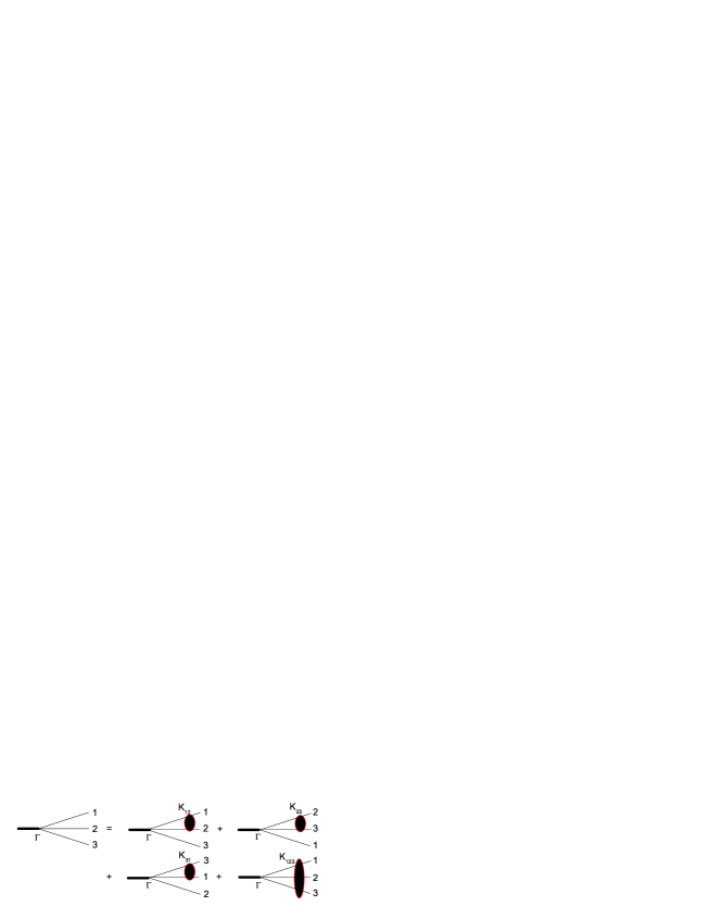
Figure 3: Three-body bound state equation with two-body and three-body forces.

Momentum conservation dictates $p_{1}+p_{2}+p_{3}=k_{1}+k_{2}+k_{3}=P$, which is enforced (on the right-hand-side) by the $\delta$-function. In the absence of intrinsic three-body kernels ($K_{123}$ in Fig. 3), the three-body bound state equation reduces to

$$\Gamma(p_{1},p_{2},p_{3};P) = \int\frac{d^{4}k}{(2\pi)^{4}}K_{12}(p_{1},p_{2};k_{1},\tilde{k}_{2};P)\;\Delta(k_{1})\;\Delta(\tilde{k}_{2})\;\Gamma(k_{1},\tilde{k}_{2},p_{3};P)$$

$$+ \int\frac{d^{4}k}{(2\pi)^{4}}K_{23}(p_{2},p_{3};k_{2},\tilde{k}_{3};P)\;\Delta(k_{2})\;\Delta(\tilde{k}_{3})\;\Gamma(p_{1},k_{2},\tilde{k}_{3};P)$$

$$+ \int\frac{d^{4}k}{(2\pi)^{4}}K_{31}(p_{3},p_{1};k_{3},\tilde{k}_{1};P)\;\Delta(k_{3})\;\Delta(\tilde{k}_{1})\;\Gamma(\tilde{k}_{1},p_{2},k_{3};P),$$

where $k_{i}=p_{i}+k$ and $\tilde{k}_{j}=p_{j}-k$ and with $K_{ij}$ the same two-body kernels as in the two-body BS equation.

2.1 Scalar three-body BS equation

For simplicity, we consider a scalar field theory, with interaction $-g\phi^{2}\varphi$, and a three-body bound state consisting of three particles $\phi$, interacting via the exchange of a $\varphi$ boson. We take equal mass $m$ for the constituents, and assume that they are all distinguishable; the mass of the exchange boson is $\mu$. In the limit $\mu=0$ this becomes the well-known Wick–Cutkosky model [19].

We use the ladder truncation for the three-body bound state equation. Furthermore, we do not take into account any self-energies (i.e. we use bare propagators). With these truncations, the three-body BS equation reduces to (see also Fig. 3)

$$\Gamma(p_{1},p_{2},p_{3};P)\;=\;g^{2}\sum\int\frac{d^{4}k}{(2\pi)^{4}}\;D(k)\;\Delta(k_{1})\;\Delta(\tilde{k}_{2})\;\Gamma(k_{1},\tilde{k}_{2},p_{3};P),$$ (3)

where $k_{i}=p_{i}+k$, $\tilde{k}_{j}=p_{j}-k$, and the sum runs (cyclic) over $i,j=1,2,3$, $i\neq j$. The propagators are: scalar constituent propagator

$$\Delta(p) = \frac{1}{p^{2}+m^{2}}\,,$$

and scalar exchange propagator

$$D(k) = \frac{1}{k^{2}+\mu^{2}}\,.$$

The momenta satisfy momentum conservation, so the three momenta $p_{i}$ are not independent. The bound state amplitude $\Gamma$ is actually function of only two (relative) independent momenta, and one can write it as a function of only two independent 4-vectors

$$\Gamma(p_{1},p_{2},p_{3};P) = \Gamma(p,q;P).$$

One can make different choices for these two relative momenta $p$ and $q$; the physics should be independent of these choices. The most natural choice are the Jacobi variables in momentum space

$$p_{1} = \mbox{$\frac{1}{3}$}P+q+p,$$

$$p_{2} = \mbox{$\frac{1}{3}$}P+q-p,$$

$$p_{3} = \mbox{$\frac{1}{3}$}P-2\,q.$$

However, this choice is not unique, and we have used other choices as well; within the estimated numerical errors, our results are independent of this choice (as it should be).

In this notation, the ladder BS equation for $\Gamma(p,q;P)$ becomes

$$\Gamma(p,q;P) = g^{2}\int\frac{d^{4}k}{(2\pi)^{4}}\;D(k)$$

$$\times \Big{[}\Delta\left(\mbox{$\frac{1}{3}$}P+q+p+k\right)\;\Delta\left(\mbox{$\frac{1}{3}$}P+q-p-k\right)\;\Gamma(p+k,q;P)$$

$$+ \phantom{\Big{[}}\Delta\left(\mbox{$\frac{1}{3}$}P+q-p+k\right)\;\Delta\left(\mbox{$\frac{1}{3}$}P-2q-k\right)\;\Gamma(p-\mbox{$\frac{1}{2}$}k,q+\mbox{$\frac{1}{2}$}k;P)$$

$$+ \phantom{\Big{[}}\Delta\left(\mbox{$\frac{1}{3}$}P-2q+k\right)\;\Delta\left(\mbox{$\frac{1}{3}$}P+q+p-k\right)\;\Gamma(p-\mbox{$\frac{1}{2}$}k,q-\mbox{$\frac{1}{2}$}k;P)\Big{]}.$$

The momentum of the exchanged particle, namely the integration variable $k$, is the same in all three terms.

2.2 Numerical implementation

As mentioned, the bound state amplitude $\Gamma$ is a function of two independent four-vectors $p$ and $q$, but the actual independent variables are: two radial variables, $p^{2}$ and $q^{2}$, and three angles, $\theta_{p}$, $\theta_{q}$, and $\phi_{pq}$. In the rest-frame of the bound state, $P_{\mu}=[i\,M,0,0,0]$, we use the notation

$$\begin{array}[]{l}p_{\mu}\;=\;p\,[\cos(\theta_{p}),\sin(\theta_{p}),0,0]\\ q_{\mu}\;=\;q\,[\cos(\theta_{q}),\sin(\theta_{q})\cos(\phi_{pq}),\sin(\theta_{q})\sin(\phi_{pq}),0]\end{array}$$

and we have the 4-dimensional integration measure

$$\int d^{4}k=\int_{0}^{\infty}k^{3}\;dk\int_{0}^{\pi}\sin^{2}(\theta)\;d\theta\int_{0}^{\pi}\sin(\phi)\;d\phi\int_{0}^{2\pi}d\gamma\,.$$

All three angular integrations have to be done numerically, in addition to the radial integration. Furthermore, we need to do some interpolation on the function $\Gamma(p,q;P)$ we are solving for, because we have expressions like $\Gamma(p-\mbox{$\frac{1}{2}$}k,q\pm\mbox{$\frac{1}{2}$}k;P)$ under the integral. Thus we have a four-dimensional integral equation for the bound state amplitude which is a function of five independent variables, given a fixed (external) $P^{2}=-M^{2}$, with a nine-dimensional kernel. For a given choice of $P^{2}=-M^{2}$ (or of the binding energy $E_{b}=3\,m-M$), we can solve this (four-dimensional) eigenvalue equation for the corresponding coupling constant $g$, or rather, for the dimensionless constant $\alpha=g^{2}/(16\pi m^{2})$; the (five-dimensional) eigenvector is the BS amplitude, $\Gamma(p^{2},q^{2},\theta_{p},\theta_{q},\phi_{pq};P^{2})$.

We solve this numerically by straightforward discretization of the internal and external variables; we do not make use of any expansion of $\Gamma$ in partial waves, nor any other set of basis functions. No matter how we re-arrange the internal and external variables, we have to do some interpolation on the function $\Gamma$ we want to solve for; that means that there is nothing to be gained by taking the internal and external grids to be the same. After a suitable transformation $q^{2}\to x$, with $0<q^{2}<\infty$, and $0<x<1$, we split the radial interval into $N$ sub-intervals, and use 2-point Gaussian integration inside each sub-interval; for the external radial grid we use the $N$ break-points (with the boundary condition that for $x=1$, i.e. $q^{2}\to\infty$ the BS amplitude vanishes). For the angular integrations we use suitable Gaussian integration measures: Gauss–Chebyshev for $\cos\theta$, Gauss–Legendre for $\cos\phi$ and $\gamma$. For the external angular variables $0<\theta_{p}<\pi$, $0<\theta_{q}<\pi$, and $0<\phi_{pq}<\pi$ and we use equidistant grids in $\cos\theta_{p,q}$ and $\cos\phi_{pq}$.

The ground state solution (that is all we are interested in right now) is symmetric under exchange of any of the three constituents. That means that $\Gamma(p,q;P)=\Gamma(-p,q;P)$, i.e. the solution we are looking for is symmetric under the combined transformation

$$\cos(\theta_{p})\;\rightarrow\;-\cos(\theta_{p}),\quad\cos(\phi_{pq})\;\rightarrow\;-\cos(\phi_{pq}).$$

Using this symmetry property saves a factor of two in the computational effort.

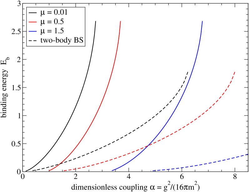
Figure 4: (Color online) Binding energies obtained by solution of the BS equation in ladder truncation for three different values of the exchange-boson mass: $\mu=0.01$, $\mu=0.5$, and $\mu=1.5$ (units set by $m=1$). Solid curves are the three-body BS result; dashed curves are the two-body BS results.

Since we are only interested in the largest eigenvalue, and its corresponding eigenvector (i.e. in the ground state), we can solve the eigenvalue equation by iteration (also called power method). Typically, we need of the order of 25 to 40 iterations in order to obtain a stable solution. Our results are shown in Fig. 4 for three different values of the mass of the exchange boson. The mass $m$ of the constituents is set to unity, so the maximal binding energy for a three-body system is three. For comparison, we also show the binding energy of the two-body system (also in ladder truncation), which clearly shows that the three-body system is stronger bound than the corresponding two-body system; i.e. the solutions we find are indeed three-body bound states.

3 Three-body bound state equation in LFD

The most simple way to derive the LF equation for spinless particles and calculate the kernel is to use the Weinberg rules [20], which are equivalent to the graph techniques in LFD [2, 3]. To calculate the amplitude $-{\cal M}$, one should put in correspondence:

• to every vertex – the factor $g$,

• to every intermediate state – the factor

  $$\frac{2}{s_{0}-s_{int}+i0},\quad\mbox{where}\quad s_{int}=\sum_{i}\frac{\vec{k}^{2}_{i\perp}+m_{i}^{2}}{x_{i}},$$

  and $s_{0}$ is the initial (=final) state energy.

In our case (three-body bound state): $s_{0}=M_{3}^{2}$, where $M_{3}$ is mass of the bound state three-body system. To every internal line one should put in correspondence the factor $\frac{\theta(x_{i})}{2x_{i}}$. One should take into account the conservation laws for $\vec{k}_{i\perp}$ and $x_{i}$ in any vertex and integrate over all independent variables with the measure $\frac{d^{2}k_{i\perp}dx_{i}}{(2\pi)^{3}}$.

Applying these rules to the graph shown in Fig. 3, we find

$$\Gamma = \int\frac{2\;\Gamma\,K_{12}}{s^{\prime}_{123}-M_{3}^{2}}\,\frac{\theta(x^{\prime}_{1})}{2x^{\prime}_{1}}\frac{\theta(x^{\prime}_{2})}{2x^{\prime}_{2}}\,\frac{d^{2}{k^{\prime}}_{1\perp}dx^{\prime}_{1}}{(2\pi)^{3}}+(231)+(312)$$

$$+ \sum\int\!\!\frac{2\,\Gamma\,K_{123}}{s^{\prime\prime}_{123}-M_{3}^{2}}\frac{\theta(x^{\prime}_{1})}{2x^{\prime}_{1}}\frac{\theta(x^{\prime}_{2})}{2x^{\prime}_{2}}\frac{\theta(x^{\prime}_{3})}{2x^{\prime}_{3}}\frac{d^{2}{k^{\prime}}_{1\perp}dx^{\prime}_{1}}{(2\pi)^{3}}\frac{d^{2}{k^{\prime}}_{3\perp}dx^{\prime}_{3}}{(2\pi)^{3}}\,.$$

Here $x^{\prime}_{1}+x^{\prime}_{2}+x_{3}=1$ in the first term, and $x^{\prime}_{1}+x^{\prime}_{2}+x^{\prime}_{3}=1$ in the last term, $s^{\prime}_{123}$ is the three-body energy in the intermediate state, with two interacting particles 12, whereas the particle 3 is free (first graph in r.h.s. of Fig. 3); $s^{\prime\prime}_{123}$ is the three-body energy in the intermediate state with all three interacting particles (last graph in r.h.s. of Fig. 3), and $\Gamma$ is the LF vertex function. The corresponding LF wave function reads

$$\psi(1,2,3)=\frac{\Gamma(1,2,3)}{s_{123}-M_{3}^{2}},$$

where

$$s_{123}=\frac{k_{1\perp}^{2}+m^{2}}{x_{1}}+\frac{k_{2\perp}^{2}+m^{2}}{x_{2}}+\frac{k_{3\perp}^{2}+m^{2}}{x_{3}}$$ (5)

with $\vec{k}_{1\perp}+\vec{k}_{2\perp}+\vec{k}_{3\perp}=0$ and sum of all $x$’s is 1, as always. $\Gamma(1,2,3)$ means: $\Gamma(1,2,3)=\Gamma(\vec{k}_{1\perp},x_{1};\vec{k}_{2\perp},x_{2};\vec{k}_{3\perp},x_{3})$ and similarly for $\psi(1,2,3)$.

Now we will use the LF Jacobi momenta $\vec{k}_{\perp}\equiv\vec{k}_{12\perp},x\equiv x_{12}$ constructed in Appendix A. I.e., we make the substitution:

$$\begin{array}[]{ll}\vec{k}_{1\perp}=\vec{k}_{\perp}-x\vec{k}_{3\perp},&x_{1}=x(1-x_{3}),\\ \vec{k}_{2\perp}=-\vec{k}_{\perp}-(1-x)\vec{k}_{3\perp},&x_{2}=(1-x)(1-x_{3}),\\ \vec{k^{\prime}}_{1\perp}=\vec{k^{\prime}}_{\perp}-x^{\prime}\vec{k^{\prime}}_{3\perp},&x^{\prime}_{1}=x^{\prime}(1-x^{\prime}_{3}),\\ \vec{k^{\prime}}_{2\perp}=-\vec{k^{\prime}}_{\perp}-(1-x^{\prime})\vec{k^{\prime}}_{3\perp},&x^{\prime}_{2}=(1-x^{\prime})(1-x^{\prime}_{3}).\end{array}$$ (6)

For $\psi$ (and $\Gamma$) we get $\psi(1,2,3)=\psi(\vec{k}_{\perp},x;\vec{k}_{3\perp},x_{3})$. Now the variables $\vec{k}_{\perp},x;\vec{k}_{3\perp},x_{3}$ are independent and they are not constrained by any relations. For both $x$’s we have: $0\leq x\leq 1$, $0\leq x_{3}\leq 1$. Then $s_{123}$, Eq. (5), becomes

$$s_{123}=\frac{k_{3\perp}^{2}+s_{12}}{1-x_{3}}+\frac{k_{3\perp}^{2}+m^{2}}{x_{3}}\ ,$$ (7)

where

$$s_{12}=\frac{k_{\perp}^{2}+m^{2}}{x(1-x)}$$

is the effective mass squared of two-body subsystem. The effective three-body mass squared $s_{123}$ has now the form of an effective mass of a two-body system, consisting of masses $\sqrt{s_{12}}$ and $m$.

In terms of Jacobi momenta, the equation for $\psi$ becomes

$$(s_{123}-M_{3}^{2})\;\psi = \int\psi\,K_{123}\;\frac{d^{2}{k^{\prime}}_{\perp}dx^{\prime}}{(2\pi)^{3}2x^{\prime}(1-x^{\prime})}\;\frac{d^{2}{k^{\prime}}_{3\perp}dx^{\prime}_{3}}{(2\pi)^{3}2x^{\prime}_{3}(1-x^{\prime}_{3})}$$ (8)

$$- \frac{m^{2}}{2\pi^{3}}\int\psi\,V_{12}\;\frac{d^{2}{k^{\prime}}_{\perp}dx^{\prime}}{(2\pi)^{3}2x^{\prime}(1-x^{\prime})(1-x_{3})}$$

$$- (231)-(312)\ .$$

Here, instead of $K_{12}$, given by the Weinberg rules, we have introduced the two-body kernel $V_{12}=-\frac{1}{4m^{2}}K_{12}=V(\vec{k^{\prime}}_{\perp},x^{\prime};\vec{k}_{\perp},x;M^{2})$, which in the non-relativistic limit turns into the potential in the Shrödinger equation. The kernel $V(\vec{k^{\prime}}_{\perp},x^{\prime};\vec{k}_{\perp},x;M^{2})$ has exactly the two-body form, i.e. the form which enters the two-body LF equation. For one-boson exchange it is given in the next section.

3.1 Scalar LF bound state equation

In ladder truncation, there is no intrinsic three-body kernel, so we omit the first term in Eq. (8) for now. However, we will find the three-body kernel $K_{123}$ due to the diagrams of Fig. 2 in Sec. 3.2 below, and calculate its contribution to the binding energy perturbatively in the next section. After omitting $K_{123}$, the LF bound state equation, Eq. (8), contains three interaction kernels $V_{12},V_{23},V_{31}$.

For the one-boson exchange model with mass $\mu$ the two-body potential reads (see e.g. [2]):

$$V(\vec{k^{\prime}}_{\perp},x^{\prime};\vec{k}_{\perp},x;M^{2})=$$ (9)

$$-\frac{4\pi\alpha}{\mu^{2}+\frac{x^{\prime}}{x}\left(1-\frac{x}{x^{\prime}}\right)^{2}m^{2}+\frac{x^{\prime}}{x}\left(\vec{k}_{\perp}-\frac{x}{x^{\prime}}\vec{k^{\prime}}_{\perp}\right)^{2}+(x^{\prime}-x)\left(\frac{m^{2}+{\vec{k^{\prime}}_{\perp}}^{2}}{x^{\prime}(1-x^{\prime})}-M^{2}\right)}\ .$$

This expression is valid for $x\leq x^{\prime}$. If $x\geq x^{\prime}$, the kernel is obtained from (9) by the permutation $x\leftrightarrow x^{\prime}$, $\vec{k}_{\perp}\leftrightarrow\vec{k^{\prime}}_{\perp}$. Here $\alpha$ is the same dimensionless coupling constant as introduced in the previous section, $\alpha={g^{2}}/{(16\pi m^{2})}$, with $g$ the coupling constant in the Hamiltonian $H=-g\phi^{2}\varphi$. In the non-relativistic limit the kernel, Eq. (9), turns into the well-known Yukawa potential

$$V(\vec{k}-\vec{k^{\prime}})=\frac{-4\pi\alpha}{\mu^{2}+(\vec{k}-\vec{k^{\prime}})^{2}}$$ (10)

which in the coordinate space is simply

$$V(r)=-\frac{\alpha e^{-\mu r}}{r}\;.$$

Now we introduce the Faddeev components

$$\psi(1,2,3) = \psi_{12}(1,2,3)+\psi_{23}(1,2,3)+\psi_{31}(1,2,3)$$ (11)

$$= \psi_{12}(1,2,3)+\psi_{12}(2,3,1)+\psi_{12}(3,1,2)\,,$$

such that the component, for instance, $\psi_{12}(1,2,3)$ satisfies an equation containing $V_{12}$ only. This procedure is standard. In this way we obtain the equation for the component $\psi_{12}$

$$(s_{123}-M_{3}^{2})\,\psi_{12}(\vec{k}_{\perp},x;\vec{k}_{3\perp},x_{3})\;=\;$$

$$\phantom{(s_{123}-M_{3}^{2})\,}-\frac{\displaystyle{m^{2}}}{\displaystyle{2\pi^{3}}}\,\displaystyle{\int}\frac{\displaystyle{d^{2}k^{\prime}_{\perp}dx^{\prime}}}{\displaystyle{2x^{\prime}(1-x^{\prime})}}\;\;\frac{\displaystyle{1}}{\displaystyle{(1-x_{3})}}\;\;V(\vec{k}_{\perp},x;\vec{k^{\prime}}_{\perp},x^{\prime};M^{2}_{12})$$

$$\times \Big{[}\psi_{12}\left(\vec{k^{\prime}}_{\perp},x^{\prime};\vec{k}_{3\perp},x_{3}\right)+\psi_{12}\left(\vec{k^{\prime}}_{23\perp},x^{\prime}_{23};\vec{k^{\prime}}_{1\perp},x^{\prime}_{1}\right)+\psi_{12}\left(\vec{k^{\prime}}_{31\perp},x^{\prime}_{31};\vec{k^{\prime}}_{2\perp},x^{\prime}_{2}\right)\Big{]}\ ,$$

where $s_{123}$ is defined by Eq. (7) and

$${M}^{2}_{12}=(1-x_{3})M_{3}^{2}-\displaystyle{\frac{k_{3\perp}^{2}+(1-x_{3})m^{2}}{x_{3}}}\ .$$ (14)

The three-body mass $M_{3}^{2}$ (which we are solving for) enters this equation through the factor $(s_{123}-M_{3}^{2})$ in l.h.s. and through the value of $M_{12}^{2}$, Eq. (14), in an argument of $V$. (An equation similar to Eq. (3.1), but for zero range interaction, was firstly derived and solved numerically in Refs. [9, 10].)

The second and third terms in Eq. (3.1), namely $\psi_{12}\left(\vec{k^{\prime}}_{23\perp},x^{\prime}_{23};\vec{k^{\prime}}_{1\perp},x^{\prime}_{1}\right)$ and $\psi_{12}\left(\vec{k^{\prime}}_{31\perp},x^{\prime}_{31};\vec{k^{\prime}}_{2\perp},x^{\prime}_{2}\right)$ depend on the LF Jacobi variables (23,1) and (31,2) respectively, whereas the equation is written in terms of the variables (12,3). The variables (23,1) and (31,2) should be expressed though (12,3). These expressions are derived in Appendix A.4. In particular, the variables $\vec{k^{\prime}}_{23\perp},x^{\prime}_{23},\vec{k^{\prime}}_{1\perp},x^{\prime}_{1}$ and $\vec{k^{\prime}}_{31\perp},x^{\prime}_{31},\vec{k^{\prime}}_{2\perp},x^{\prime}_{2}$ are obtained from Eqs. (33) and (34) of Appendix A.4 by the replacement: $\vec{k}_{\perp}\to\vec{k^{\prime}}_{\perp}$, $x\to x^{\prime}$. To be specific:

$$\begin{array}[]{ll}\vec{k}^{\prime}_{23\perp}=\displaystyle{-\frac{x_{3}\vec{k}^{\prime}_{\perp}+(1-x^{\prime})\vec{k}_{3\perp}}{1-x^{\prime}+x^{\prime}x_{3}}},&x^{\prime}_{23}=\displaystyle{\frac{(1-x^{\prime})(1-x_{3})}{1-x^{\prime}+x^{\prime}x_{3}}},\\ &\\ \vec{k^{\prime}}_{1\perp}=\vec{k^{\prime}}_{\perp}-x^{\prime}\vec{k}_{3\perp},&x^{\prime}_{1}=x^{\prime}(1-x_{3}),\end{array}$$ (15)

and

$$\begin{array}[]{ll}\vec{k^{\prime}}_{31\perp}=\displaystyle{-\frac{x_{3}\vec{k^{\prime}}_{\perp}-x^{\prime}\vec{k}_{3\perp}}{x^{\prime}+x_{3}-x^{\prime}x_{3}}},&x^{\prime}_{31}=\displaystyle{\frac{x_{3}}{x^{\prime}+x_{3}-x^{\prime}x_{3}}},\\ &\\ \vec{k^{\prime}}_{2\perp}=-\vec{k^{\prime}}_{\perp}-(1-x^{\prime})\vec{k}_{3\perp},&x^{\prime}_{2}=(1-x^{\prime})(1-x_{3}).\end{array}$$ (16)

With this notation (and omitting prime), the full wave function obtains the form:

$$\psi(\vec{k}_{\perp},x;\;\vec{k}_{3\perp},x_{3}) = \psi_{12}(\vec{k}_{\perp},x;\;\vec{k}_{3\perp},x_{3})$$

$$+ \psi_{12}(\vec{k}_{23\perp},x_{23};\;\vec{k}_{1\perp},x_{1})+\psi_{12}(\vec{k}_{31\perp},x_{31};\;\vec{k}_{2\perp},x_{2})\ .$$

It is normalized as

$$\int\big{|}\psi(\vec{k}_{\perp},x;\vec{k}_{3\perp},x_{3})\big{|}^{2}\;\frac{d^{2}k_{\perp}dx}{(2\pi)^{3}2x(1-x)}\;\frac{d^{2}k_{3\perp}dx_{3}}{(2\pi)^{3}2x_{3}(1-x_{3})}\;=\;1\ .$$ (18)

3.2 Contribution from three-body kernel

Naively, one might not expect any three-body kernels in the ladder truncation. However, in LFD, there are three-body kernels, as already mentioned in the introduction, due to the (LF) time-ordering of the diagrams. To find the correction to the binding energy from the kernel $K_{123}$, we represent equation for the full wave function symbolically in the form

$$(s_{123}-M_{3}^{2})\psi = (\hat{K}_{12}+\hat{K}_{23}+\hat{K}_{31})\psi+\hat{K}_{123}\psi\,.$$

Substituting $M_{3}^{2}\to M_{3}^{2}+\Delta M_{3}^{2}$, we find

$$\Delta M_{3}^{2} = -(\psi\hat{K}_{123}\psi),$$

or, explicitly

$$\Delta M^{2}_{3}=\;-\int\frac{d^{2}k_{3\perp}}{(2\pi)^{3}}\;\frac{d^{2}k_{\perp}}{(2\pi)^{3}}\;\frac{d^{2}k^{\prime}_{3\perp}}{(2\pi)^{3}}\;\frac{d^{2}k^{\prime}_{\perp}}{(2\pi)^{3}}$$

$$\times\int_{0}^{1}\frac{dx_{3}}{2x_{3}(1-x_{3})}\;\frac{dx}{2x(1-x)}\;\frac{dx^{\prime}_{3}}{2x^{\prime}_{3}(1-x^{\prime}_{3})}\;\frac{dx^{\prime}}{2x^{\prime}(1-x^{\prime})}$$

$$\times\psi(\vec{k}_{\perp},x;\vec{k}_{3\perp},x_{3})\,K_{123}(\vec{k}_{\perp},x;\vec{k}_{3\perp},x_{3};\vec{k^{\prime}}_{\perp},x^{\prime};\vec{k^{\prime}}_{3\perp},x^{\prime}_{3})\,\psi(\vec{k^{\prime}}_{\perp},x^{\prime};\vec{k^{\prime}}_{3\perp},x^{\prime}_{3})\,.$$

The integrand depends on four 2-dimensional vectors $\vec{k}_{\perp}$, $\vec{k}_{3\perp}$, $\vec{k^{\prime}}_{\perp}$, $\vec{k^{\prime}}_{3\perp}$ and, hence, on three relative angles between them. Therefore Eq. (3.2) is an 11-dimensional integral (the last, fourth angle integration, is reduced to a factor $2\pi$).

The kernel $K_{123}$ is determined by 54 graphs: 48 of them contain two exchange-bosons in flight, whereas another 6 correspond to the intermediate production of a pair of constituent particle-antiparticles. It is sufficient to calculate only the nine graphs shown in Fig. 2. The other contributions are obtained by permutations and can be taken into account by multiplying the results of these nine graphs by a factor 3!=6.

Here we show explicitly how to calculate the contribution of the first graph Fig. 2 only. All other contributions are calculated in a similar fashion. Following the Weinberg rules [20], we get

$$K^{(1)}_{123}=\frac{2^{8}\pi^{2}m^{4}\alpha^{2}}{(s_{1}-M_{3}^{2})\,(s_{2}-M_{3}^{2})\,(s_{3}-M_{3}^{2})}\frac{\theta(x_{1}-x^{\prime}_{1})}{(x_{1}-x^{\prime}_{1})}\,\frac{\theta(x^{\prime}_{1}+x^{\prime}_{2}-x_{1})}{(x^{\prime}_{1}+x^{\prime}_{2}-x_{1})}\,\frac{\theta(x_{3}-x^{\prime}_{3})}{(x_{3}-x^{\prime}_{3})}\,,$$ (20)

where $s_{i}$ are the energies in intermediate states shown in Fig. 2. The line 1, for instance, is associated with the momenta $\vec{k}_{1\perp},x_{1}$ and contributes in $s_{1}$ the term $\frac{k_{1\perp}^{2}+m^{2}}{x_{1}}$, and analogously for other lines. We sum over all the lines in given intermediate state. In this way we find for $s_{1}$:

$$s_{1}=\frac{k_{1\perp}^{2}+m^{2}}{x_{1}}+\frac{k_{2\perp}^{2}+m^{2}}{x_{2}}+\frac{(\vec{k}_{3\perp}-\vec{k^{\prime}}_{3\perp})^{2}+\mu^{2}}{x_{3}-x^{\prime}_{3}}+\frac{{k^{\prime}}^{2}_{3\perp}+m^{2}}{x^{\prime}_{3}}\,.$$

Other intermediate state energies can be found similarly. Transforming this expression to the LF Jacobi variables by the substitution (6), we find:

$$s_{1}=\frac{(\vec{k}_{3\perp}-\vec{k^{\prime}}_{3\perp})^{2}+\mu^{2}}{x_{3}-x^{\prime}_{3}}+\frac{\vec{k}\,^{2}_{\perp}+x(1-x)\vec{k}\,^{2}_{3\perp}+m^{2}}{x(1-x)(1-x_{3})}+\frac{\vec{k^{\prime}}\,^{2}_{3\perp}+m^{2}}{x^{\prime}_{3}}\,.$$

The final expression for the kernel $K^{(1)}_{123}$ is obtained by substitution of this expression for $s_{1}$ (and analogously, for $s_{2},s_{3}$) in Eq. (20) and replacing also the variables $x$’s in Eq. (20) by the Jacobi ones according to Eqs. (6). The $\theta$-functions impose the following constrains on the Jacobi’s $x$’s:

$$0\leq x_{3}\leq 1,\qquad 0\leq x\leq 1,\qquad 0\leq x^{\prime}_{3}\leq x_{3},$$

and

$$0\leq x^{\prime}\leq\frac{x(1-x_{3})}{1-x^{\prime}_{3}}\,.$$

Other contributions are found similarly. All of them have the form (20) with the replacement of $s_{1},s_{2},s_{3}$ by the corresponding twelve intermediate energies $s_{1}-s_{12}$, as shown in the various graphs in Fig. 2, and also $x$’s in the $\theta$-functions and in denominator. Taking the sum of all the contributions and substituting it in Eq. (3.2), we find the perturbative correction to the binding energy resulting from the three-body forces:

$$\Delta M_{3}^{2} = -6\int\frac{d^{2}k_{3\perp}}{(2\pi)^{3}}\;\frac{d^{2}k_{\perp}}{(2\pi)^{3}}\;\frac{d^{2}k^{\prime}_{3\perp}}{(2\pi)^{3}}\;\frac{d^{2}k^{\prime}_{\perp}}{(2\pi)^{3}}\int_{0}^{1}\frac{dx_{3}}{2x_{3}(1-x_{3})}\int_{0}^{1}\frac{dx}{2x(1-x)}$$ (21)

$$\times \Bigg{\{}\int_{0}^{x_{3}}\frac{dx^{\prime}_{3}}{2x^{\prime}_{3}(1-x^{\prime}_{3})}$$

$$\times \Bigg{[}\int_{0}^{\frac{x(1-x_{3})}{1-x^{\prime}_{3}}}\frac{\psi(K^{(1)}_{123}+K^{(2)}_{123})\psi^{\prime}\;dx^{\prime}}{2x^{\prime}(1-x^{\prime})}+\int_{\frac{x(1-x_{3})}{1-x^{\prime}_{3}}}^{\frac{1-x_{3}}{1-x^{\prime}_{3}}}\frac{\psi(K^{(3)}_{123}+K^{(4)}_{123})\psi^{\prime}\;dx^{\prime}}{2x^{\prime}(1-x^{\prime})}\Bigg{]}$$

$$+ \phantom{\Bigg{\{}}\int_{x_{3}}^{1-x(1-x_{3})}\!\!\!\!\!\!\frac{dx^{\prime}_{3}}{2x^{\prime}_{3}(1-x^{\prime}_{3})}$$

$$\times \Bigg{[}\int_{0}^{\frac{x(1-x_{3})}{1-x^{\prime}_{3}}}\frac{\psi(K^{(5)}_{123}+K^{(6)}_{123})\psi^{\prime}\;dx^{\prime}}{2x^{\prime}(1-x^{\prime})}+\int_{\frac{x(1-x_{3})}{1-x^{\prime}_{3}}}^{1}\frac{\psi(K^{(7)}_{123}+K^{(8)}_{123})\psi^{\prime}\;dx^{\prime}}{2x^{\prime}(1-x^{\prime})}\Bigg{]}$$

$$+ \int_{0}^{x_{3}}\frac{dx^{\prime}_{3}}{2x^{\prime}_{3}(1-x^{\prime}_{3})}\int_{\frac{1-x_{3}}{1-x^{\prime}_{3}}}^{1}\frac{\psi K^{(9)}_{123}\psi^{\prime}\;dx^{\prime}}{2x^{\prime}(1-x^{\prime})}\Bigg{\}}\ .$$

The three-body wave function $\psi$ is expressed through the Faddeev component $\psi_{12}$ by Eq. (3.1), whereas $\psi_{12}$ is found from Eq. (3.1); $\psi$ and $\psi^{\prime}$ depend on the variables $\vec{k}_{\perp},x;\;\vec{k}_{3\perp},x_{3}$ and $\vec{k^{\prime}}_{\perp},x^{\prime};\;\vec{k^{\prime}}_{3\perp},x^{\prime}_{3}$ respectively.

4 Numerical results

The LF wave functions in Eq. (3.1) depend on five independent scalar variables. The wavefunction $\psi_{12}(\vec{k}_{\perp},x;\vec{k}_{3\perp},x_{3})$ on the l.h.s. of Eq. (3.1) depends on the external variables $k_{\perp}$, $k_{3\perp}$, $x$, $x_{3}$, and $z=\cos\beta=\vec{k}_{\perp}\cdot\vec{k}_{3\perp}/(k_{\perp}k_{3\perp})$. The arguments of the wave functions $\psi$’s in the integrand on the r.h.s. of Eq. (3.1) can be expressed through a combination of these five external variables and the three integration variables $k^{\prime}_{\perp}$, $x^{\prime}$, and $\cos\beta^{\prime}=\vec{k}_{\perp}\cdot\vec{k^{\prime}}_{\perp}/(k_{\perp}k^{\prime}_{\perp})$. Thus the structure of the LF bound state equation, Eq. (3.1), is very similar to that of the BS equation, Eq. (2.1), and we can solve it in a similar fashion. That is, we use a transformation to map the radial variable onto a finite interval, discretize all five variables, and perform all integrations numerically (three in the case of LFD, four in the case of the BS equation).

4.1 Difference between BS approach and LFD

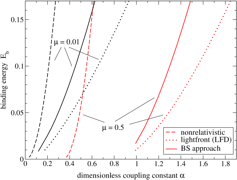
Figure 5: (Color online) Three-body binding energy in the limit when it tends to zero, for $\mu=0.01$ and $\mu=0.5$ (units set by the constituent mass: $m=1$). Solid curves are the BS result; dotted curves are the LFD results; dashed curves are the solution of the non-relativistic Schrödinger equation.

For small binding energies, our results for the three-body binding energies $E_{b}=3m-M_{3}$ are shown in Fig. 5 (the units are set by $m=1$). For comparison, we also include the non-relativistic result obtained by solving the non-relativistic Schödinger equation (solved via corresponding non-relativistic Faddeev equation in the momentum space with the kernel Eq. (10)). Clearly, all three calculations give different results.

However, the relativistic binding energies, calculated using the BS equation and in LFD, are approaching to each other as the binding energy goes to zero. Unfortunately, the numerics become less accurate in that limit, because both the interaction kernels and the wave functions we are solving for become more peaked. Nevertheless, for $\mu=0.5$, within numerical accuracy, they appear to have the same critical coupling, defined as the coupling constant $\alpha$ at which the binding energy becomes zero. In contrast, the non-relativistic binding energy behaves quite differently, and vanishes at a much smaller value of $\alpha$.

This behavior is similar to that which was found in the two-body system [4]. In the latter case, the decreasingly small binding energies, calculated via relativistic (both BS equation and LFD) and non-relativistic equations, become close to each other only in the limit $\mu\to 0$.

Indeed, for the value $\mu=0.01$ in Fig. 5, the relativistic and non-relativistic results approach each other as all the binding energies decrease down to $E_{b}\approx 0.01$, and they seem to extrapolate to $\alpha\approx 0$ as the point at which the binding energy becomes zero. We did not calculate for smaller $E_{b}$ and $\mu$ because of increasing numerical errors.

More intriguing is the rather large difference we see in this figure between the results from the BS equation and those from LFD for nonzero binding energy $E_{b}$. The LF equation in ladder truncation significantly underbinds the three-body system relative to the ladder BS equation. Though at small binding, both BS and LFD binding energies tend to each other and to zero, the relative difference between them remains significant, and is roughly a factor of two. We remind the reader that for two-body system these binding energies approximately coincide with each other [4].

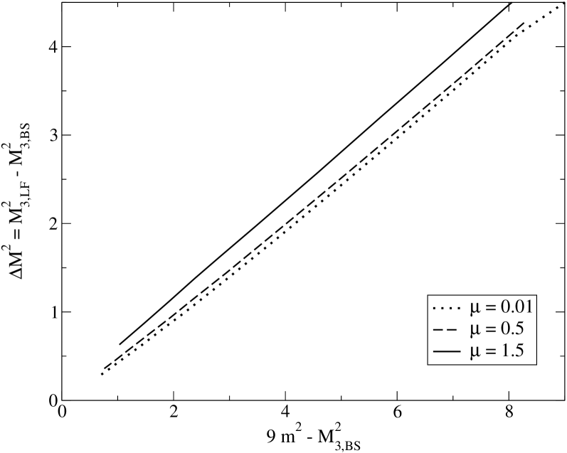
Figure 6: (Color online) The difference $M_{3,LF}^{2}-M_{3,BS}^{2}$ vs. the deviation of $M_{3,BS}^{2}$ from the free value: $9m^{2}-M_{3,BS}^{2}$, for different values of the exchange mass $\mu$.

A closer look at our results reveals that the difference between the three-body masses squared in the BS approach and in LFD, $M_{3,LF}^{2}-M_{3,BS}^{2}$, is approximately proportional to $M_{3,BS}^{2}$ itself. In Fig 6, we show the difference

$$\Delta M^{2}=M_{3,LF}^{2}-M_{3,BS}^{2}$$

as function of $9m^{2}-M_{3,BS}^{2}$. It is a remarkably linear function over the entire accessible interval of $M_{3,BS}^{2}$ (remember: $9m^{2}-M_{3}^{2}=0$ means zero binding energy, and $M_{3}^{2}=0$ is the maximal binding energy); furthermore, it depends only weakly on $\mu$, the mass of the exchange boson.

4.2 Differences largely explained by 3-body force

The next question is: Can this difference between the BS approach and LFD be explained by the diagrams of Fig. 2? In order to answer this question, we performed a perturbative calculation of the correction to $M_{3,LF}^{2}$ due to these three-body forces, using Eq. (21). In Fig. 7 we show our results for the contributions both from the diagrams with two exchange-bosons in flight (first eight graphs in Fig. 2) and from the diagrams with creation and annihilation of an intermediate particle-antiparticle pair (ninth graph in in Fig. 2). Since this calculation involves the numerical evaluation of an 11-dimensional integral, see Eq. (3.2), the results are not highly accurate; nevertheless, they are quite illustrative.

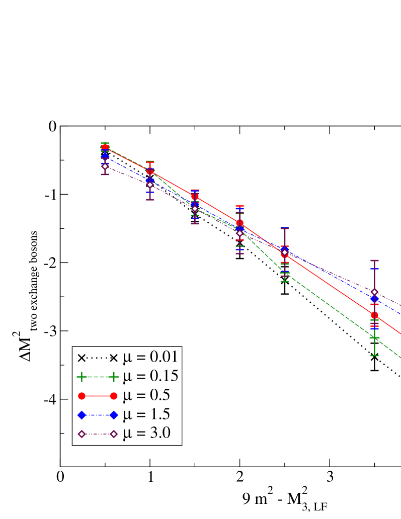
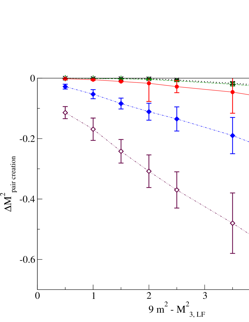
Figure 7: (Color online) Correction $\Delta M_{3}^{2}$, Eq. (21), vs. the difference $9m^{2}-M^{2}_{3,LFD}$ for different values of the exchange mass $\mu$. Top: Contributions from the first eight graphs in Fig. 2 (without pair-creation); Bottom: Contributions from pair-creation only, the last diagram in Fig. 2. Notice the difference in the vertical scale.

As we can see in the top panel of Fig. 7, the contribution of two exchange-bosons in flight to $\Delta M_{3}^{2}$ is an almost linear function of $M_{3}^{2}$. Furthermore, it depends only very weakly on the value of $\mu$ in the wide interval $0.01\leq\mu\leq 3.0$.

The contribution of the pair creation term only (ninth graph in Fig. 2) is shown in the bottom panel of Fig. 7. Again, it is almost linear in $M_{3}^{2}$, but, in contrast to two exchange-bosons in flight, it strongly depends on $\mu$. At $\mu=3.0$ this contribution is about 20% relative to two exchange-bosons in flight but it becomes negligible for $\mu\leq 0.15$.

The behavior of these both contributions is consistent with the behavior of the difference of the masses squared in the BS and LFD approaches, Fig. 6. This linearly increasing (in absolute value) negative correction from effective three-body forces in LFD eliminates most, if not all, of the linearly increasing positive difference between BS and LFD results.

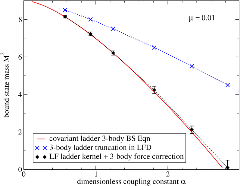
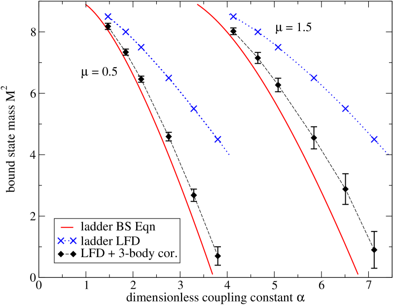
Figure 8: (Color online) Three-body bound state mass squared $M_{3}^{2}$ vs. coupling constant $\alpha$ for exchange masses $\mu=0.01$ (top), $0.5$ and $1.5$ (bottom). The units are set by the constituent mass: $m=1$.

The three-body bound state mass squared $M_{3}^{2}$ for the exchange masses $\mu=0.01$, $0.5$ and $1.5$ are shown in Fig. 8. Like in Fig. 5, the solid and dotted curves are our results from the three-body BS equation in ladder truncation, Eq. (2.1), and our results from the LF 3-body bound state equation with the two-body one-boson exchange kernel, Eq. (9), respectively. As in Fig. 5, the BS and LFD results differ significantly from each other and the difference increases with increase of the binding energy (and, hence, with the coupling constant).

The crosses on the dotted curves indicate the points where we evaluated the perturbative correction due the 3-body forces depicted in Fig. 2. The diamonds with error bars in Fig. 8 indicate the sum $M_{3,LF}^{2}+\Delta M_{3}^{2}$, where $\Delta M_{3}^{2}$ is the correction due from the diagrams of Fig. 2, calculated perturbatively by Eq. (21), and displayed in Fig. 7. The errors indicate the numerical uncertainty, mainly due to the numerical evaluation of an 11-dimensional integral. This correction does indeed shift the LFD three-body mass squared so that it comes in reasonably good agreement with the BS results. This is the effect of relativistic three-body forces, dominated here by two exchange-bosons in flight, with a small contribution from the creation (and annihilation) of a pair of constituent particle-antiparticles.

One should of course keep in mind that here we only present a perturbative estimate of the correction due to these effective 3-body forces in LFD. Note that the perturbative calculation is unexpectedly good even for large correction compared to the value of $M^{2}$ itself, especially for small values $\mu$ of the mass of the exchange particle. The agreement becomes less pronounced as the exchange mass increases, once the exchange mass becomes larger than the constituent mass. E.g. if the exchange mass is three times the constituent mass, the perturbative correction explains about 70% of the difference in $M_{3}^{2}$ between the BS approach and LFD.

Since the corrections are substantial, one could raise the question: How is a perturbative calculation reliable in this context? To answer this question, one should solve equation (8) beyond the perturbative framework, which is numerically much more demanding and requires significantly more work. Nevertheless, we have ample evidence that the contributions of effective 3-body forces in LFD are substantial in the three-body systems, and can explain most of the difference between the results found in the BS approach and in LFD.

5 Conclusion

We have solved, for the first time, the three-body BS and LFD bound state equations with a one-boson exchange kernel and found a difference in the corresponding binding energies. This difference is absent in the two-body BS and LFD equations [4].

When the binding energies tend to zero, the absolute difference between BS and LFD results decreases too. However, the difference of the binding energies relative to the binding energy itself remains roughly constant: LFD in ladder truncation underbinds approximately by a factor of two, compared to the ladder BS equation. The relative difference depends only weakly on the exchange-boson mass $\mu$. At the same time, the difference between the relativistic BS (or LFD) binding energies on one hand, and the binding energy found from a purely non-relativistic approach on the other hand, is much larger than the difference between the BS approach and LFD. In particular the critical coupling for the onset of bound states in a three-body system appears to be the same in the BS approach and in LFD, but in a non-relativistic calculation this critical coupling is significantly smaller. This difference decreases with the decrease of the exchange-boson mass; in the limit of a massless exchange boson, this critical coupling tends to zero for all three approaches. The latter is quite similar to two-body calculations, where one also finds a significant difference between a purely non-relativistic calculation on the one hand, and the BS equation or LFD on the other hand.

Most of the difference between BS and LFD three-body binding energies can be attributed to effective 3-body forces. Despite the fact that both in the BS approach and in LFD we use an one-boson exchange kernel, the actual kernels in the three-body BS and LFD bound state equations differ from each other by contributions of irreducible LFD graphs with two exchange-bosons in flight and by pair creation. Both types of graphs are implicitly included in the ladder kernel of the BS equation (this becomes obvious if its iterations are transformed in a set of the time-ordered diagrams), but they are not included in the one-boson exchange kernel in LFD. In the latter case they should be taken into account separately, as an extra contribution from a 3-body force. After taking them into account perturbatively, the LFD binding energy becomes approximately equal to the BS results, at least for exchange masses smaller than the constituent mass ($\mu<m$). This is a clear manifestation of three-body forces, which in our model are unambiguously given by the set of graphs Fig. 2 and explicitly calculated.

Three-body forces of this origin contribute only to the kernel of 3-dimensional bound state equations, like the LFD one. They can also be taken into account as a relativistic correction in the framework of the Schrödinger three-body equation (together with other relativistic corrections). They are true three-body forces in a 3-dimensional framework. However, in the framework of the BS equation, using 4-dimensional integral equations and explicitly covariant variables without any 3-dimensional reduction, these effects are automatically incorporated via iterations of the two-body ladder kernel. They do not manifest themselves as three-body forces in the BS approach. Therefore, the interpretation of forces as two- or three-body forces, depends on the framework with which these forces are associated.

Note that three-body forces, resulting from excitations of intermediate isobar states, do not depend on the type of equation: BS, LFD or Schrödinger equation. They remain three-body forces in any of these equations. However, they may turn into two-body forces if one considers the intermediate isobars in the framework of a system of coupled channel equations, including transitions $N\leftrightarrow\Delta$. Both types of these three-body forces could be taken into account as a correction to a non-relativistic treatment of nuclei.

In addition, there can be intrinsic three-body forces, such as the six-nucleon contact term $NNN\to NNN$, generated by chiral perturbation theory for the effective nucleon interaction at the N2LO level [21], or, in QCD, three-body forces due to the triple gluon vertex. However, these intrinsic three-body forces are beyond the skope of the present paper.

We would like to emphasize that although we find a correction to the LFD kernel (three-body forces) which explains most of the difference between the LFD binding energy and the BS binding energy, this does not mean that LFD is considered as an approximate method to solve the BS equation. Both the BS approach and LFD have their advantages and disadvantages. Without truncations, they should give the same results for physical quantities such as the bound state mass. However, truncations can lead to differences between LFD and the BS approach. A detailed comparison between results obtained in LFD and in the BS approach, such as the work presented here, provides deeper insight in the limitations and deficiencies of the truncation. Here, it revealed that for three-body bound states in the ladder truncation in LFD there are significant contributions to the binding energy coming from effective three-body forces related to higher Fock sectors.

Finally, the calculations presented here have been done for spinless systems: a scalar bound state, composed of three scalar constituents, interacting via exchange of a scalar boson. Physical systems such as the triton and ³He nuclei, or baryons as bound states of three quarks, consist of fermions, interacting via (pseudo-)scalar and/or vector bosons. We expect that at least qualitatively our conclusions hold for those systems as well: For three-body systems, the ladder truncation of the Bethe–Salpeter equation and the ladder truncation in light-front dynamics are not equivalent, and are likely to give significantly different results, due to the absence of diagrams like those in Fig. 2 in the light-front ladder truncation.

Appendix A LF Jacobi variables

The three-body LF wave function depends on the variables $\vec{k}_{1\perp},\vec{k}_{2\perp},\vec{k}_{3\perp}$ and $x_{1},x_{2},x_{3}$. Because of conservation of momenta, they are not independent, but satisfy the relations: $\vec{k}_{1\perp}+\vec{k}_{2\perp}+\vec{k}_{3\perp}=0$, $x_{1}+x_{2}+x_{3}=1$.

For any sub-system ($\alpha\beta$) we define corresponding LF Jacobi variables, which are independent from each other.

A.1 Sub-system 12

For subsystem 12 we introduce the Jacobi momenta as follows:

$$\begin{array}[]{lcl}x_{12}&=&\frac{x_{1}}{x_{1}+x_{2}}\ ,\cr\vec{k}_{12\perp}&=&\vec{k}_{1\perp}-x_{12}(\vec{k}_{1\perp}+\vec{k}_{2\perp})\ .\end{array}$$ (22)

The construction of $x_{12}$ agrees with general definition of variable $x$: for subsystem 12 it is the ratio $x_{12}=\frac{p_{1+}}{p_{12+}}$, where $p_{12+}=p_{1+}+p_{2+}$ is the plus-component of the four-momentum of the subsystem 12. Dividing numerator and denominator by the plus-component of the total three-body momentum $p_{+}\equiv p_{0}+p_{z}=p_{1+}+p_{2+}+p_{3+}$, we find for $x_{12}$ expression (22) in terms of the variables $x_{1},x_{2}$ defined for three-body system.

One can express them as follows

$$\begin{array}[]{lcl}x_{12}&=&\frac{x_{1}}{1-x_{3}}\ ,\cr\vec{k}_{12\perp}&=&\vec{k}_{1\perp}+\frac{x_{1}}{1-x_{3}}\vec{k}_{3\perp}\end{array}$$ (23)

and vice versa:

$$x_{1}=x_{12}(1-x_{3}),\quad\vec{k}_{1\perp}=\vec{k}_{12\perp}-x_{12}\vec{k}_{3\perp}.$$

The Faddeev component $\psi_{12}$ becomes a function of

$$\psi_{12}=\psi_{12}(\vec{k}_{12\perp},x_{12};\vec{k}_{3\perp},x_{3}).$$

In contrast to the variables $x_{1},x_{2},x_{3}$, constrained by $x_{1}+x_{2}+x_{3}=1$, both variables $x_{12},x_{3}$ vary independently in the interval from 0 to 1.

The three-body integration measure, with integration over two-body subsystem, is transformed as:

$$\delta^{(2)}(\vec{k^{\prime}}_{1\perp}+\vec{k^{\prime}}_{2\perp}+\vec{k}_{3\perp})\delta(x^{\prime}_{1}+x^{\prime}_{2}+x_{3}-1)\frac{d^{2}k^{\prime}_{1\perp}dx^{\prime}_{1}d^{2}k^{\prime}_{2\perp}dx^{\prime}_{2}}{2x^{\prime}_{1}x^{\prime}_{2}}$$

$$= \delta^{(2)}(\vec{k^{\prime}}_{12\perp}+\vec{k^{\prime}}_{21\perp})\delta(x^{\prime}_{12}+x^{\prime}_{21}-1)\frac{1}{(1-x_{3})}\frac{d^{2}k^{\prime}_{12\perp}dx^{\prime}_{12}d^{2}k^{\prime}_{21\perp}dx^{\prime}_{21}}{2x^{\prime}_{12}x^{\prime}_{21}}$$

$$\Rightarrow \frac{1}{(1-x_{3})}\,\frac{d^{2}k^{\prime}_{12\perp}dx^{\prime}_{12}}{2x^{\prime}_{12}(1-x^{\prime}_{12})}\ .$$

In the non-relativistic limit $x_{12}\approx 1/2$, $x_{3}\approx 1/3$, and we obtain usual Jacobi coordinates:

$$\vec{k}_{12\perp} \approx \vec{k}_{1\perp}-\frac{1}{2}(\vec{k}_{1\perp}+\vec{k}_{2\perp})=\frac{1}{2}(\vec{k}_{1\perp}-\vec{k}_{2\perp}),$$

$$\vec{k}_{3\perp} \approx \vec{k}_{1\perp}-\frac{1}{3}(\vec{k}_{1\perp}+\vec{k}_{2\perp}+\vec{k}_{3\perp})=\frac{2}{3}\left[\vec{k}_{1\perp}-\frac{1}{2}(\vec{k}_{2\perp}+\vec{k}_{3\perp})\right].$$ (25)

A.2 Sub-system 23

Corresponding formulas are obtained from the relations for the 12-subsystem by the cyclic permutation $123\to 231$. Then the Jacobi variables are defined as follows:

$$\begin{array}[]{lcl}x_{23}&=&\frac{x_{2}}{x_{2}+x_{3}}\ ,\cr\vec{k}_{23\perp}&=&\vec{k}_{2\perp}-x_{23}(\vec{k}_{2\perp}+\vec{k}_{3\perp})\ .\end{array}$$ (26)

One can express them as functions of the three-body variables

$$\begin{array}[]{lcl}x_{23}&=&\frac{x_{2}}{1-x_{1}}\ ,\cr\vec{k}_{23\perp}&=&\vec{k}_{2\perp}+\frac{x_{2}}{1-x_{1}}\vec{k}_{1\perp}\end{array}$$ (27)

and vice versa:

$$x_{2}=x_{23}(1-x_{1}),\quad\vec{k}_{2\perp}=\vec{k}_{23\perp}-x_{23}\vec{k}_{1\perp}.$$ (28)

The Faddeev component $\psi_{23}$ becomes a function of

$$\psi_{23}=\psi_{23}(\vec{k}_{23\perp},x_{23};\vec{k}_{1\perp},x_{1}).$$

A.3 Sub-system 31

Corresponding formulas are obtained from the relations for the 23-subsystem by the cyclic permutation $123\to 231$ or from the relations for the 12-subsystem by the cyclic permutation $123\to 312$. Then the Jacobi variables are defined as follows:

$$\begin{array}[]{lcl}x_{31}&=&\frac{x_{3}}{x_{3}+x_{1}}\ ,\cr\vec{k}_{31\perp}&=&\vec{k}_{3\perp}-x_{31}(\vec{k}_{3\perp}+\vec{k}_{1\perp})\ .\end{array}$$ (29)

One can also introduce $x_{13}=1-x_{31},\vec{k}_{13\perp}=-\vec{k}_{31\perp}$.

One can express them as functions of the three-body variables

$$\begin{array}[]{lcl}x_{31}&=&\frac{x_{3}}{1-x_{2}}\ ,\cr\vec{k}_{31\perp}&=&\vec{k}_{3\perp}+\frac{x_{3}}{1-x_{2}}\vec{k}_{2\perp}\end{array}$$ (30)

and vice versa:

$$x_{3}=x_{31}(1-x_{2}),\quad\vec{k}_{3\perp}=\vec{k}_{31\perp}-x_{31}\vec{k}_{2\perp}.$$ (31)

The Faddeev component $\psi_{31}$ becomes a function of

$$\psi_{31}=\psi_{31}(\vec{k}_{31\perp},x_{31};\vec{k}_{2\perp},x_{2}).$$

A.4 Relation between different Jacobi coordinates and cyclic permutations

We express the coordinates for the subsystems 23 and 31 in terms of 12: $x_{12},\vec{k}_{12\perp},x_{3},\vec{k}_{3\perp}$. For that we substitute in the above formulas the Eqs. (A.1) and use the relations:

$$\begin{array}[]{ll}x_{1}=\displaystyle{x_{12}(1-x_{3})},&\vec{k}_{1\perp}=\vec{k}_{12\perp}-x_{12}\vec{k}_{3\perp},\\ &\\ x_{2}=1-x_{12}(1-x_{3})-x_{3},&\vec{k}_{2\perp}=-(\vec{k}_{12\perp}-x_{12}\vec{k}_{3\perp})-\vec{k}_{3\perp}.\end{array}$$ (32)

Then we find:

$$\begin{array}[]{ll}x_{23}=\displaystyle{\frac{(1-x_{12})(1-x_{3})}{1-x_{12}+x_{12}x_{3}}},&\vec{k}_{23\perp}=\displaystyle{-\frac{x_{3}\vec{k}_{12\perp}+(1-x_{12})\vec{k}_{3\perp}}{1-x_{12}+x_{12}x_{3}}},\\ &\\ x_{1}=x_{12}(1-x_{3}),&\vec{k}_{1\perp}=\vec{k}_{12\perp}-x_{12}\vec{k}_{3\perp}.\end{array}$$ (33)

and

$$\begin{array}[]{ll}x_{31}=\displaystyle{\frac{x_{3}}{x_{12}+x_{3}-x_{12}x_{3}}},&\vec{k}_{31\perp}=\displaystyle{-\frac{x_{3}\vec{k}_{12\perp}-x_{12}\vec{k}_{3\perp}}{x_{12}+x_{3}-x_{12}x_{3}}}\ ,\\ &\\ x_{2}=(1-x_{12})(1-x_{3}),&\vec{k}_{2\perp}=-\vec{k}_{12\perp}-(1-x_{12})\vec{k}_{3\perp}\ .\end{array}$$ (34)

After cyclic permutation $123\to 231$ the variables $\vec{k}_{12\perp},x_{12}$ turn into $\vec{k}_{23\perp},x_{23}$ defined by Eqs. (33), and similarly for other variables and permutations. In this way one obtains Eq. (3.1) for total wave function. Note that the transformations of the $x$-variables are non-linear, since they are defined through $x_{1},x_{2},x_{3}$ by the non-linear formulas (22), (26), (29).

References

• [1] Maris, P., Roberts, C.D.: Int. J. Mod. Phys. E12, 297 (2003) [arXiv:nucl-th/0301049].
• [2] Carbonell, J., Desplanques, B., Karmanov, V.A., Mathiot, J.-F.: Phys. Reports, 300, 215 (1998) [arXiv:nucl-th/9804029]
• [3] Brodsky, S., Pauli, H-C., Pinsky, S.: Phys. Reports, 301, 299 (1998) [arXiv:hep-ph/9705477]
• [4] Mangin-Brinet, M., Carbonell, J.: Phys. Lett., B474, 237 (2000) [arXiv:nucl-th/9912050]
• [5] Karmanov, V.A., Carbonell, J., Mangin-Brinet, M.: Nucl. Phys. A790, 598c, (2007) [arXiv:hep-th/0610158]; Few-Body Systems (to be published) [arXiv:0712.0971 (hep-ph)]
• [6] Dorkin, S.M., Beyer, M., Semikh, S.S., Kaptari, L.P.: Few-Body Systems 42, 1 (2008) [arXiv:0708.2146v1 (nucl-th)]
• [7] Mangin-Brinet, M., Carbonell, J., Karmanov, V.A.: Phys. Rev. C68, 055203 (2003) [arXiv:hep-th/0308179]
• [8] Maris, P.: Two and three-body bound states in an explicitly covariant framework, presented at the international workshop LC2006: Light Cone QCD and nonperturbative hadron physics, Minneapolis, USA, May 15-19, 2006
• [9] Frederico, T.: Phys. Lett. B282, 409 (1992)
• [10] Carbonell, J., Karmanov, V.A.: Phys.Rev. C67, 037001 (2003) [arXiv:nucl-th/0207073]
• [11] Lin, T., Elster, Ch., Polyzou, W.N., Witala, H., Gloeckle, W.: [arXiv:0801.3210 (nucl-th)]; Lin, T., Elster, Ch., Polyzou, W.N., Gloeckle, W.: Phys. Rev. C76, 014010 (2007) [arXiv:nucl-th/0702005]; Witala, H., Golak, J., Skibinski, R., Glockle, W., Polyzou, W.N., Kamada, H.: Phys. Rev. C77, 034004 (2008) [arXiv:0801.0367 (nucl-th)]
• [12] Schoonderwoerd, N.C.J., Bakker, B.L.G., Karmanov, V.A.: Phys. Rev. C58, 3093 (1998) [arXiv:nucl-th/9806365]
• [13] Carbonell, J., Karmanov, V.A.: Eur. Phys. J. A27, 11 (2006); [arXiv:hep-th/0505262]
• [14] Friar, J.L.: Nucl. Phys. A684, 200 (2001) [arXiv:nucl-th/9911075]
• [15] Shirokov, A.M., Vary, J.P., Mazur, A.I., Weber, T.A.: Phys. Letts. B644, 33 (2007) [arXiv:nucl-th/0512105]
• [16] Brueckner, K.A., Levinson, C.A., Mahmoud, H.M.: Phys. Rev. 95, 217 (1954)
• [17] Shin-Nan Yang; Phys. Rev. C10, 2067 (1974)
• [18] Shin-Nan Yang, Glöckle, W.: Phys. Rev. C33, 1774 (1986)
• [19] Wick, G.C.: Phys. Rev. 96, 1124 (1954)
Cutkosky, R.E.: Phys. Rev. 96, 1135 (1954)
• [20] Weinberg, S.: Phys. Rev. 150, 1313 (1966)
• [21] Entem, D.R., Machleidt, R.: Phys. Rev. C68, 041001 (2003) [arXiv:nucl-th/0304018]