Ground-state properties of interacting two-component Bose gases in a hard-wall trap

Abstract

We investigate ground-state properties of interacting two-component Bose gases in a hard-wall trap using both the Bethe ansatz and exact numerical diagonalization method. For equal intra- and inter-atomic interaction, the system is exactly solvable. Thus the exact ground state wavefunction and density distributions for the whole interacting regime can be obtained from the Bethe ansatz solutions. Since the ground state is a degenerate state with total spin $S=N/2$, the total density distribution are same for each degenerate state. The total density distribution evolves from a Gauss-like Bose distribution to a Fermi-like one as the repulsive interaction increases. The distribution of each component is $N_{\alpha}/N$ of the total density distribution. This is approximately true even in the experimental situation. In addition the numerical results show that with the increase of interspecies interaction the distributions of two Tonks-Girardeau gases exhibit composite fermionization crossover with each component developing N peaks in the strongly interacting regime.

I Introduction

Since two-component Bose-Einstein condensates (BECs) of trapped alkali atomic clouds were realized experimentally Myatt ; Erhard , low-dimensional multi-component Bose gases have attracted much attention from theory and experiment due to their connection to many areas of physics. Theoretical investigation mainly focuses on the stability, phase separation, collective excitation, Josephson-type oscillations and other macroscopic quantum many-body phenomena Ho96 ; Ao ; Pu ; Cazalilla ; Williams in the frame work of mean field theory. Other fundamental problems such as topological defects, symmetry breaking effects also attract growing interest symmetry ; Timmermans .

Advances in experiment with ultracold atoms provide exciting opportunities to control and manipulate ultracold atom gases in one-dimensional (1D) waveguides by tightly confining the atomic cloud in two radial directions and weakly confining it along the axial direction Stoeferle ; Paredes ; Toshiya . Successful realization of 1D interacting quantum degenerate gases enables us to study novel many-body effect in various of interacting regimes, for example, in the strongly interacting limit, i.e. the Tonks-Girardeau (TG) gases Girardeau . Tunability of the scattering length cross Feshbach resonance allows experimentalists access to whole interaction regime from a weakly interacting limit to a strongly interacting limit. Strong correlation effect in 1D quantum degenerate gases Olshanii have been extensively studied in recent years Olshanii2 ; Petrov ; Dunjko ; Chen ; delcampo . It is shown that 1D quantum systems exhibit particular features which are significantly different from its three dimensional counterpart.

The exact results for single component bosons with a repulsive $\delta$-function interaction show that the density profiles evolve from Gaussian-like distribution of Bosons to shell-structured distribution of Fermions when interaction strength increases Hao06 ; Hao07 ; Deuretzbacher ; Zoellner ; Cederbaum ; Yin . In order to study the system in the strong interacting regime, non-perturbation method is highly desirable and reliable because the mean field theory is proven to be insufficient. For the multi-component quantum gases, studies were carried out by means of various schemes such as mean field theory Ho96 ; Ao ; Pu ; Cazalilla , extended Bose-Fermi mapping in the infinitely repulsive limit Girardeau07 ; DeuretzbacherPRL ; Guan ; Hao08 ; Zoellner08 and exact Bethe ansatz LiYQ ; Gusj ; Guan07 ; Fuchs . The 1D homogeneous two-component Bose gas with spin-independent $s$-wave scattering (equal inter- and intra-species interacting strengthes) is exactly solvable by the Bethe ansatz method in a whole physical regime LiYQ ; Gusj . The ferromagnetic ordering in spinor Bose gases was predicted some years ago Eisenberg ; Yang . However, the system is no longer integrable if the atomic gas no longer has the $SU(2)$ symmetry or it is trapped in an inhomogeneous potential. In this situation numerical methods have to be exerted and rich phenomena are shown for various parameters Zoellner08 ; Hao08 .

Previous study on the integrable two-component Bose gas mainly focuses on the energy spectrum and excitation properties LiYQ ; Guan07 ; Gusj ; Fuchs . However, important quantities, which are related to the wave function of the system and are accessible experimentally, such as the density distribution and momentum distribution, are rarely addressed except in the limit of infinitely repulsive interaction Girardeau07 . In this paper, we are aimed to study the two-component bosonic systems with $SU(2)$ symmetry in the whole interacting regime by means of the Bethe ansatz. In the case of broken $SU(2)$ symmetry, we resort to exact diagonalization method. The total density distribution and the density distribution for each component can be derived from exact ground state wave function. In addition, numerical method will be used to evaluate the reduced one-body density matrix and momentum distribution of each component as well as inter- and intra-species density-density correlations.

The present paper is organized as follows. Section II introduces the model and gives the exact solutions by means of the Bethe ansatz for the integrable point. In Section III the numerical diagonalization method is introduced and we investigate the system for accessible experimental parameters after checking the accuracy of the numerical result. Section IV is devoted to the interaction of two TG gases. A summary is given in the last section.

II Exact solution of two-component Bose gas

We consider two-component Bose gas confined in a 1D hard wall trap of length $L$, which is composed of two internal states (pseudospin $\left|\uparrow\right\rangle$ and $\left|\downarrow\right\rangle$ denote state 1 and 2, respectively) of the same kind of Bose atoms with equal mass $m_{1}=m_{2}=m$. The atom numbers in each component are $N_{1}$ and $N_{2}$ and $N=N_{1}+N_{2}$ the total number. The many body system can be described by the second quantized Hamiltonian

$$\mathcal{H} = \int dx\sum_{\alpha=1,2}\left\{\frac{\hbar^{2}}{2m_{\alpha}}\frac{\partial\hat{\Psi}_{\alpha}^{\dagger}(x)}{\partial x}\frac{\partial\hat{\Psi}_{\alpha}(x)}{\partial x}\right.$$

$$\left.+\frac{g_{\alpha}}{2}\hat{\Psi}_{\alpha}^{\dagger}(x)\hat{\Psi}_{\alpha}^{\dagger}(x)\hat{\Psi}_{\alpha}(x)\hat{\Psi}_{\alpha}(x)\right\}$$

$$+g_{12}\int dx\hat{\Psi}_{1}^{\dagger}(x)\hat{\Psi}_{2}^{\dagger}(x)\hat{\Psi}_{2}(x)\hat{\Psi}_{1}(x),$$

where $g_{\alpha}$ ($\alpha=1,2$) and $g_{12}$ denote the effective intra- and inter-species interaction which can be controlled experimentally by tuning the corresponding scattering lengthes $a_{1}$, $a_{2}$ and $a_{12}$, respectively. The field operator $\Psi_{\alpha}^{\dagger}(x)$ ($\Psi_{\alpha}(x)$) creates (annihilates) an $\alpha$-component boson at the position $x$. A standard rescaling procedure brings the Hamiltonian into a dimensionless one

$$\mathcal{H} = \int dx\sum_{\alpha}\left\{\hat{\Psi}_{\alpha}^{\dagger}(x)\left[-\frac{\partial^{2}}{\partial x^{2}}+U_{\alpha}\hat{\Psi}_{\alpha}^{\dagger}\hat{\Psi}_{\alpha}\right]\hat{\Psi}_{\alpha}(x)\right\}$$ (1)

$$+2U_{12}\int dx\hat{\Psi}_{1}^{\dagger}(x)\hat{\Psi}_{2}^{\dagger}(x)\hat{\Psi}_{2}(x)\hat{\Psi}_{1}(x)$$

with $U_{\alpha}=mg_{\alpha}/\hbar^{2}$ ($\alpha=1,2,12$). Here we have rescaled the energy and length in units of $\hbar^{2}/2mL^{2}$ and $L$. The system with equal interaction constants $U_{1}=U_{2}=U_{12}=c$ is integrable in both the periodic boundary LiYQ and open boundary conditions Gusj ; Guan07 and the eigen problem for the original Hamiltonian is reduced to solving the coordinate nonlinear Schrödinger equation

$$H\Psi\left(x_{1},\cdots,x_{N}\right)=E\Psi\left(x_{1},\cdots,x_{N}\right)$$ (2)

with

$$H=-\sum_{j=1}^{N}\frac{\partial^{2}}{\partial x_{j}^{2}}+2c\sum_{j<l}\delta(x_{j}-x_{l}).$$ (3)

The Hamiltonian $H$ commutes with the total spin operator $\hat{S}$, i.e., commutes with all the three components of the total spin operator, so that they share a common set of eigenstates and the system possesses a global SU(2) symmetry. Explicitly, the three components of total spin operator are defined as

$$\hat{S}^{\alpha}=\frac{1}{2}\int dx\sum_{\mu,\nu}\hat{\Psi}_{\mu}^{\dagger}(x)\sigma^{\alpha}_{\mu,\nu}\hat{\Psi}_{\nu}(x),$$

where $\mu,\nu\in\{\uparrow,\downarrow\}$ with $\uparrow$ ($\downarrow$) corresponding to the $1$th component ($2$th component) and $\sigma^{\alpha}$ ($\alpha=x,y,z$) denotes the Pauli matrices.

The coordinate wave function can be determined by means of Bethe ansatz method and takes the following general form

$$\Psi\left(x_{1},\cdots,x_{N}\right)$$ (4)

$$= \sum_{P,Q}\theta\left(x_{q_{N}}-x_{q_{N-1}}\right)\cdots\theta\left(x_{q_{2}}-x_{q_{1}}\right)\times$$

$$\sum_{r_{1},\ldots,r_{N}}\left[A\left(Q,rP\right)\exp\left(i\sum_{j}r_{p_{j}}k_{p_{j}}x_{q_{j}}\right)\right],$$

where $Q=(q_{1},q_{2},\cdots,q_{N})$ and $P=(p_{1},p_{2},\cdots,p_{N})$ are one of the permutations of $1,\cdots,N$, respectively, $A\left(Q,rP\right)$ is the abbreviation of the coefficient $A\left(q_{1},q_{2},\cdots,q_{N};r_{p_{1}}p_{1},r_{p_{2}}p_{2},\cdots,r_{p_{N}}p_{N}\right)$ to be determined self-consistently, and the summation $\sum_{P}$ ($\sum_{Q}$) is done for all of them. Here $r_{j}=\pm$ indicates that the particles move toward the right or the left, $\theta(x-y)$ is the step function and the parameters $\left\{k_{j}\right\}$ are known as quasi-momenta. Moreover the wavefunction Eq. (4) should fulfill the the open boundary condition Gaudin for hard wall trap

$$\Psi\left(\cdots,x_{j}=0,\cdots\right)=\Psi\left(\cdots,x_{j}=L,\cdots\right)=0,$$

which enforces the relations

$$A\left(Q;\cdots,-p_{i},\cdots,r_{p_{N}}p_{N}\right)=-A\left(Q;\cdots,p_{i},\cdots,r_{p_{N}}p_{N}\right).$$

Furthermore, the coefficients fulfill the general relations

$$A(Q;\cdots i,j\cdots)=Y_{ji}^{ab}A(Q;\cdots j,i\cdots)$$

with $Y_{ji}^{ab}$ given by

$$Y_{ji}^{ab}=\frac{(k_{j}-k_{i})P_{q_{a}q_{b}}-ic}{k_{j}-k_{i}+ic},$$

where $P_{q_{a}q_{b}}$ is the permutation operator on $A(\cdots q_{a},q_{b},\cdots;P)$ so that it interchanges $q_{a}$ and $q_{b}$ Gusj ; LiYQ ; Guan07 ; YangCN . For the eigenstate with total spin $S=N/2-M$ ($0\leq M\leq N/2$), the Bethe ansatz equations Gusj ; Guan07 satisfied by the quasi-momentum {$k_{j}$} and spin rapidity {$\Lambda_{\alpha}$} are given by

$$\exp(2ik_{j}L) = \prod_{l=1\neq j}^{N}\left(\frac{k_{j}-k_{l}+ic}{k_{j}-k_{l}-ic}\frac{k_{j}+k_{l}+ic}{k_{j}+k_{l}-ic}\right)\times$$

$$\prod_{\alpha=1}^{M}\left(\frac{k_{j}-\Lambda_{\alpha}-ic^{\prime}}{k_{j}-\Lambda_{\alpha}+ic^{\prime}}\frac{k_{j}+\Lambda_{\alpha}-ic^{\prime}}{k_{j}+\Lambda_{\alpha}+ic^{\prime}}\right),$$

$$\prod_{l=1}^{N}\left(\frac{\Lambda_{\alpha}-k_{l}-ic^{\prime}}{\Lambda_{\alpha}-k_{l}+ic^{\prime}}\frac{\Lambda_{\alpha}+k_{l}-ic^{\prime}}{\Lambda_{\alpha}+k_{l}+ic^{\prime}}\right)$$

$$= \prod_{\beta\neq\alpha}^{M}\left(\frac{\Lambda_{\alpha}-\Lambda_{\beta}-ic}{\Lambda_{\alpha}-\Lambda_{\beta}+ic}\frac{\Lambda_{\alpha}+\Lambda_{\beta}-ic}{\Lambda_{\alpha}+\Lambda_{\beta}+ic}\right),$$

with $c^{\prime}=c/2$. The energy eigenvalue is $E=\sum_{j=1}^{N}k_{j}^{2}$. Taking the logarithm of Bethe ansatz equations, we have

$$k_{j}L = \pi I_{j}-\sum_{l=1}^{N}\left(\tan^{-1}\frac{k_{j}-k_{l}}{c}+\tan^{-1}\frac{k_{j}+k_{l}}{c}\right)$$ (5)

$$+\sum_{\alpha=1}^{M}\left(\tan^{-1}\frac{k_{j}-\Lambda_{\alpha}}{c^{\prime}}+\tan^{-1}\frac{k_{j}+\Lambda_{\alpha}}{c^{\prime}}\right),$$

$$\sum_{j=1}^{N}\left(\tan^{-1}\frac{\Lambda_{\alpha}-k_{j}}{c^{\prime}}+\tan^{-1}\frac{\Lambda_{\alpha}+k_{j}}{c^{\prime}}\right)$$

$$= \pi J_{\alpha}+\sum_{\beta\neq\alpha}^{M}\left(\tan^{-1}\frac{\Lambda_{\alpha}-\Lambda_{\beta}}{c}+\tan^{-1}\frac{\Lambda_{\alpha}+\Lambda_{\beta}}{c}\right).$$

Here the quantum numbers $I_{j}$ and $J_{\alpha}$ take integer or half-integer values, depending on whether $N-M$ is odd or even. The ground state corresponds to the case with $M=0$ LiYQ ; Gusj ; Guan07 ; Fuchs . For the ground state $I_{j}=\left(N+1\right)/2-j$ and $J_{\alpha}$ is an empty set, and the Bethe ansatz equations reduce to the situation of Lieb-Liniger Bose gas. In this case, the coefficient $A(Q;p_{1},p_{2},\cdots,p_{N})$ can be explicitly expressed as

$$A(Q;p_{1},p_{2},\cdots,p_{N})$$

$$= (-1)^{P}\prod_{j<l}^{N}(ik_{p_{l}}-ik_{p_{j}}+c)(ik_{p_{l}}+ik_{p_{j}}+c),$$

with $(-1)^{P}=\pm 1$ denoting sign factors associated with even or odd permutations of $P=(p_{1},p_{2},\cdots,p_{N})$. By numerically solving the sets of transcendental equations eq.(5), the quasimomentum $\left\{k_{j}\right\}$ and thus the ground state wavefunction can be determined exactly.

For the two-component Bose gas with SU(2) symmetry, it has been proven that the ground states are $\left(N+1\right)$-fold degenerate isospin ‘ferromagnetic’ states LiYQ ; Gusj ; Eisenberg ; Yang , which are symmetrical under permutation of any two spins. Among the degenerate ground states, the fully polarized state can be represented as

$$\left|\Psi^{N}\left(\frac{N}{2},\frac{N}{2}\right)\right\rangle = \int d^{N}\mathbf{x}~{}\Psi\left(x_{1},\cdots x_{N}\right)\times$$ (6)

$$\hat{\Psi}_{\uparrow}^{\dagger}(x_{1})\hat{\Psi}_{\uparrow}^{\dagger}(x_{2})\cdots\hat{\Psi}_{\uparrow}^{\dagger}(x_{N})\left|0\right\rangle,$$

where $\Psi\left(x_{1},\cdots x_{N}\right)$ is given by the Bethe ansatz ground-state wave function (4). Other degenerate states can be generated by applying the total lowering operator $\hat{S}^{-}$ to the polarized state. For example, the total ground state wave function for the degenerate ground state with $N_{2}$ spin-down particles (the state with $S=N/2$ and $S_{z}=(N_{1}-N_{2})/2$) can be expressed as

$$\left|\Psi^{N}\left(\frac{N}{2},\frac{N_{1}-N_{2}}{2}\right)\right\rangle=\left(\hat{S}^{-}\right)^{N_{2}}\left|\Psi^{N}\left(\frac{N}{2},\frac{N}{2}\right)\right\rangle,$$ (7)

where the total lowering spin operator $\hat{S}^{-}$ is defined as $\hat{S}^{-}=\frac{1}{2}\int dx\hat{\Psi}_{\downarrow}^{\dagger}(x)\hat{\Psi}_{\uparrow}(x)$ .

Figure 1: (color online) The ground-state density distribution of the first component for (a) $N_{1}=4,N_{2}=0$, (b)$N_{1}=3,N_{2}=1$, (c)$N_{1}=2,N_{2}=2$, (d)$N_{1}=1,N_{2}=3$, and $c=0,5,15,50$.

In terms of the ground state wave function $\Psi\left(x_{1},\cdots,x_{N}\right)$ the total density distribution $\rho_{\text{tot}}(x)=\sum_{\alpha=1,2}\rho_{\alpha}(x)$ can be expressed as

$$\rho_{\text{tot}}(x)=\frac{N\int_{0}^{L}dx_{2}\cdots dx_{N}\left|\Psi\left(x,x_{2},\cdots,x_{N}\right)\right|^{2}}{\int_{0}^{L}dx_{1}\cdots dx_{N}\left|\Psi\left(x_{1},x_{2},\cdots,x_{N}\right)\right|^{2}}.$$

Here the ground-state density distribution of the $\alpha$-component is given by

$$\rho_{\alpha}(x)=\left\langle\Psi^{N}\left(S,S_{z}\right)\right|\hat{\Psi}_{\alpha}^{\dagger}(x)\hat{\Psi}_{\alpha}(x)\left|\Psi^{N}\left(S,S_{z}\right)\right\rangle.$$

From the explicit form of the many body wavefunction, it is straightforward to get the ground-state density distribution of the $\alpha$-component which is found to fulfill a simple relation with the total density distribution (see Appendix)

$$\rho_{\alpha}(x)=\frac{N_{\alpha}}{N}\rho_{\text{tot}}(x).$$ (8)

We obtain unique total density profiles for all configurations with the same total atom number $N$: $\left[N_{1},N_{2}\right]=\left[N,0\right],\left[N-1,1\right],\ldots\left[0,N\right]$, which is also confirmed by the numerical exact diagonalization method in the later evaluation. The conclusion (8) is valid for the integrable two-component boson system in the whole regime of repulsive interaction. Moreover, we would like to indicate that the conclusion (8) is valid even in the presence of an external confinement if the system has the total SU(2) symmetry, i.e., the case with $U_{1}=U_{2}=U_{12}$ note . We thus recover the result in Ref. Girardeau07 where only infinitely repulsive limit was considered by a generalized Bose-Fermi mapping method.

In the following calculation, $L=1$ will be used through the paper. In Fig. 1 we display the the ground-state density distributions of the first component for $N=4$ and $N_{2}=0,1,2,3$ for different interacting constants, where we find similar crossover behavior as those of a single component Bose gas. When the interaction is weak the density profiles show Gaussian-like distribution and in the strongly interacting regime the density profiles exhibit a shell structure with $N$ peaks for each component. In the intermediate interacting regime the distribution show obvious evolution from Bose distribution to Fermi distribution. According to eq.(8), each component takes the same density profiles and is normalized to the atom number in the component. Therefore, all configurations with the same total atom number share the same total density distribution. It is worth to note the absence of the demixing in the integrable system, which is contrary to prediction of a mean field approximation.

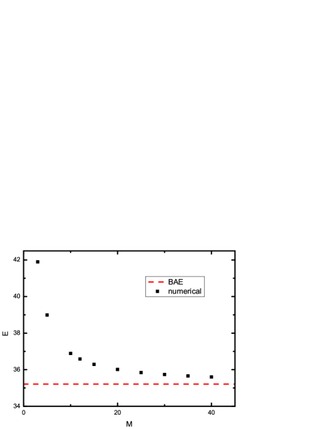
Figure 2: (color online) The ground state energy for $c=10$ and $N=4$ vs utilized orbital number. Dashed line: The exact result of Bethe ansatz method; Scatters: Numerical diagonalization results. Units of energy: $\hbar^{2}/2mL^{2}$.

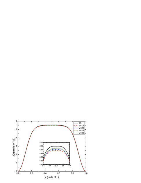
Figure 3: (color online) Density distribution of the ground state for $c=10$ and $N=4$. Inset: enlarged profiles in $x\in[0.3,0.7]$.

III Numerical Diagonalization Method

Although the system is integrable for the situation of equal intra- and inter-atomic interactions and some exact results can be obtained in this case, we have to turn to the numerical method when the system deviates from the integrable point. In fact it is very difficult to adjust the intra- and inter-atomic interactions to be exactly the same in the realization of experiment. For instance the scattering lengths and thus the effective 1D interaction constants are known to be in the proportion $U_{1}:U_{12}:U_{2}=1.03:1:0.97$ in the two components of Bose gas composed of internal states $\left|F=1,m_{f}=-1\right\rangle$ and $\left|F=2,m_{f}=1\right\rangle$ in ⁸⁷Rb atoms scaleg . In this situation Bethe ansatz method is not applicable and we resort to the numerical exact diagonalization method.

Let us first briefly review the numerical diagonalization method and then investigate the ground state properties of the Bose-Bose mixture. The normalized eigen wavefunction (orbital) of one particle in a hard wall takes the form $\phi_{i}(x)=\sqrt{\frac{2}{L}}\sin\left(\frac{i\pi}{L}x\right)$, upon which the field operator $\Psi_{\alpha}(x)$ can be expanded as

$$\Psi_{\alpha}(x)=\sum_{i=0}^{\infty}\phi_{i}(x)\hat{b}_{i\alpha}.$$

The operator $\hat{b}_{i\alpha}^{\dagger}$ ($\hat{b}_{i\alpha}$) creates (annihilates) one $\alpha$-component atom in the $i-$th orbital. As a result the Hamiltonian (1) is discretized as

$$H = \sum_{\alpha=1,2}\left[\sum_{i}\mu_{i}\hat{b}_{i\alpha}^{\dagger}\hat{b}_{i\alpha}+{U_{\alpha}}\sum_{i,j,k,l}I_{i,j,k,l}\hat{b}_{i\alpha}^{\dagger}\hat{b}_{j\alpha}^{\dagger}\hat{b}_{k\alpha}\hat{b}_{l\alpha}\right]$$ (9)

$$+2U_{12}\sum_{i,j,k,l}I_{i,j,k,l}\hat{b}_{i1}^{\dagger}\hat{b}_{j2}^{\dagger}\hat{b}_{k2}\hat{b}_{l1}$$

with $\mu_{i}=\left(i\pi\right)^{2}$ ($i=1,2,3,...$) and the dimensionless integrals $I_{ijkl}=\int_{0}^{L}dx\phi_{i}(x)\phi_{j}(x)\phi_{k}(x)\phi_{l}(x)$. The dimension of the Hilbert space is now $C_{N_{1}+M-1}^{N_{1}}\times C_{N_{2}+M-1}^{N_{2}}$ if $N_{1}$ 1-component atoms and $N_{2}$ 2-component atoms are populated on $M$ orbitals. Then the ground state $\left|\text{GS}\right\rangle$ can be obtained after diagonalizing the Hamiltonian in the Hilbert space spanned by the one-particle eigenstates. In order to assure the precision of evaluation sufficient orbitals should be considered particularly for the systems in strongly interacting regime. The total density distribution is given by

$$\rho_{\text{tot}}(x)=\sum_{\alpha=1}^{2}\rho_{\alpha}(x)$$

with the density distribution of $\alpha$-component

$$\rho_{\alpha}(x) = \left\langle\text{GS}\right|{\Psi}_{\alpha}^{\dagger}(x){\ \Psi}_{\alpha}(x)\left|\text{GS}\right\rangle$$ (10)

$$= \sum_{i,j}\phi_{i}^{*}(x)\phi_{j}(x)\left\langle\text{GS}\right|\hat{b}_{i\alpha}^{\dagger}\hat{b}_{j\alpha}\left|\text{GS}\right\rangle.$$

In terms of the ground state wave function the reduced one-body density matrix for each component and the two body correlation of intra- and inter-species atom can be formulated as

$$\rho_{\alpha}(x,x^{\prime}) = \left\langle\text{GS}\right|{\Psi}_{\alpha}^{\dagger}(x){\ \Psi}_{\alpha}(x^{\prime})\left|\text{GS}\right\rangle$$ (11)

$$= \sum_{i,j}\phi_{i}^{*}(x)\phi_{j}(x^{\prime})\left\langle\text{GS}\right|\hat{b}_{i\alpha}^{\dagger}\hat{b}_{j\alpha}\left|\text{GS}\right\rangle$$

and

$$\rho_{\alpha\beta}(x,x^{\prime})$$

$$= \left\langle\text{GS}\right|{\Psi}_{\alpha}^{\dagger}(x){\ \Psi}_{\alpha}(x){\Psi}_{\beta}^{\dagger}(x^{\prime}){\ \Psi}_{\beta}(x^{\prime})\left|\text{GS}\right\rangle$$

$$= \sum_{i,j,k,l}\phi_{i}^{*}(x)\phi_{j}(x)\phi_{k}^{*}(x^{\prime})\phi_{l}(x^{\prime})\left\langle\text{GS}\right|\hat{b}_{i\alpha}^{\dagger}\hat{b}_{j\alpha}\hat{b}_{k\beta}^{\dagger}\hat{b}_{l\beta}\left|\text{GS}\right\rangle.$$

The momentum distribution is simply the Fourier transformation of $\rho_{\alpha}(x,x^{\prime})$,

$$n_{\alpha}\left(k\right)=\frac{1}{2\pi}\int_{0}^{L}dx\int_{0}^{L}dx^{\prime}\rho_{\alpha}(x,x^{\prime})e^{-ik\left(x-x^{\prime}\right)}.$$ (13)

In order to test the accuracy of our numerical code, we compare the numerical result with that from Bethe ansatz method on calculating the ground state energy and total density profiles of two components Bose gas with $N=4$. The results are shown in Fig. 2 and Fig. 3 for an intermediate interaction constant $c=10$. The ground state energy is shown to asymptotically approach the BA result $E/N=35.22$ if sufficient orbitals are taken into account. For instance, we have the ground state energy $E/N=35.60$ for $M=40$, the deviation of which is already within $1\%$. The density profiles calculated for $M=15$ can match the BA result very well. In the following calculation, the orbital number is taken as $M=20$ ($M=15$) for $N=4$ $(N=5)$ and the reduced Hilbert space is typically composed of $10^{4}$ basis states with a corresponding energy cutoff $(M\pi)^{2}=3947.84$ $(2220.66)$.

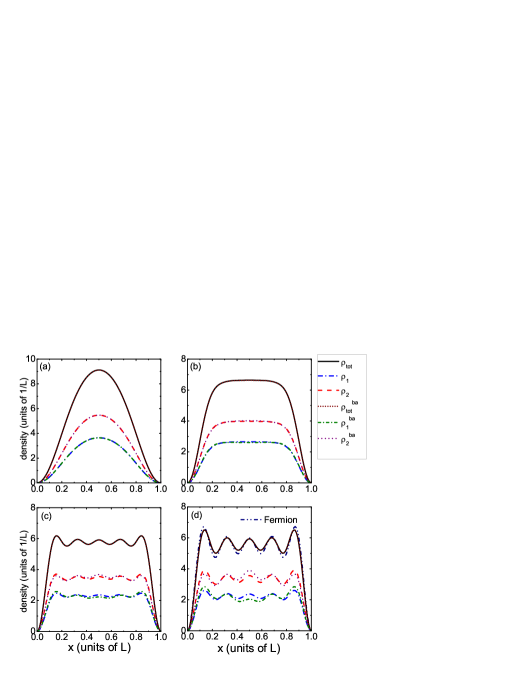
Figure 4: (color online) Density distribution of the ground state for $N_{1}=2,N_{2}=3$ and $U=1.0(a),10.0(b),40.0(c),80.0(d)$. $\rho_{\alpha}^{\text{BA}}(\alpha=1,2,\text{tot})$: Bethe-Ansatz result for equal intra- and inter-atomic interactions ($U_{1}=U_{2}=U_{12}=U$); $\rho_{\alpha}(\alpha=1,2,\text{tot})$: Numerical result for unequal intra- and inter-atomic interactions ($U_{1}:U_{12}:U_{2}=1.03:1:0.97$).

Using the numerical method the density profiles of each component can be obtained even for unequal atom numbers and $SU(2)$ symmetry broken atomic interaction constants, i.e. $U_{1}\neq U_{2}\neq U_{12}$. In Fig 4. we display both the total density distribution and the that of each component in the full interacting regime for equal and unequal intra- and inter-atomic interactions in the case of $N_{1}=2,N_{2}=3$. In the situation of unique interaction constant, two components display the same density distribution in the full interacting regime, i.e., $\rho_{\alpha}(x)=\frac{N_{\alpha}}{N}\rho_{\text{tot}}(x)$. The density profiles show evolution from Bose to Fermi distribution with the increase of atomic interaction. In Fig. 4d we compare the distribution of the system of finite strong interaction with the distribution of TG gas, which is obtained using the Bose-Fermi mapping. It turns out that even if the interaction is finite the result from Bose-Fermi mapping can describe the system very well. Generally the ground state energy and the density profiles of two-component Bose gas do not show distinct difference from its single component counterpart. For unequal intra- and inter-atomic interacting constants as in the experiment ($U_{1}:U_{12}:U_{2}=1.03:1:0.97$), the density profiles do not change drastically comparing with those of integrable system even in the strongly interacting regime. Particularly in the weakly interacting regime, the exact solution of integrable system provides a trustable description of the real experimental system because of the relatively small asymmetry of the intra- and inter-species interacting constants .

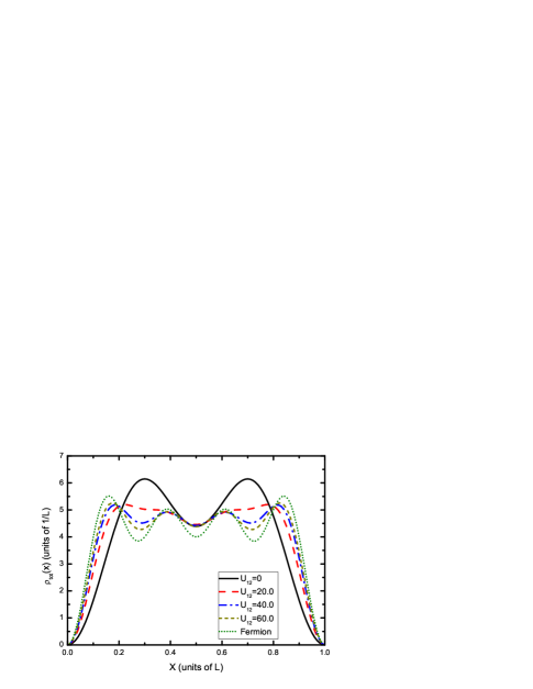
Figure 5: (color online) Density distribution of the ground state for $N_{1}=N_{2}=2$ and $U_{1}=U_{2}=60$.

IV Interaction between two TG gases

We have shown that how the fermionization crossover for the one-component Bose gas extends to a two-component mixture in the whole repulsive regime with almost equal intra- and inter-atomic interactions. The numerical diagonalization method can be used to investigate two components of Bose gases even when there are great difference between the intra- and inter-atomic interactions. Now we focus on the crossover induced by the inter-atomic interaction constants. We start with the case with $U_{12}=0$ and $U_{1}=U_{2}=60$, where each component is an independent TG gas, and increase the inter-atomic interaction $U_{12}$ to see how the composite fermionization crossover happens for two initially fermionized components. In Fig. 5 the total density profiles are given for $N_{1}=N_{2}=2$ and $U_{1}=U_{2}=60$. In this situation the distributions of each component match each other and they are one half of the total distribution because of equal atom numbers in two components. When the inter-atomic interaction disappear the system is composed of two isolated TG gases that display $N_{\alpha}$ peaks. With the increase of inter-atomic interaction the density profiles become flatter with more peaks appearing. In the strongly interacting limit the shell structure with $N$ peaks display, which is the same as the density profiles of single component of TG gas of $N$ atoms. For the 1D Bose-Bose mixtures under harmonic confinement, such a composite-fermionization crossover has been observed as the interspecies coupling strength is varied to the limit of infinite repulsion Zoellner08 ; Hao08 .

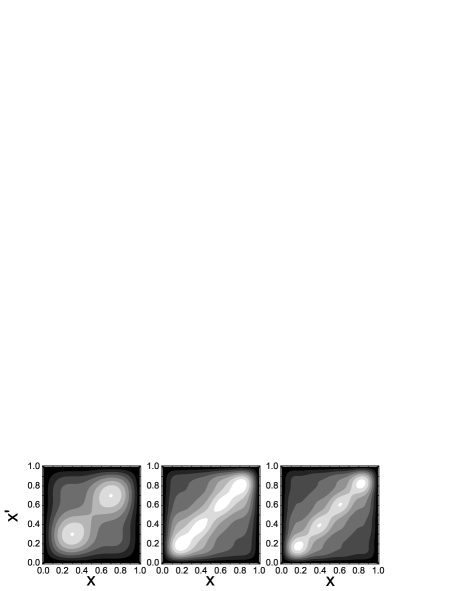
Figure 6: The reduced one body density matrix for each component of the ground state for $N_{1}=N_{2}=2$ and $U_{1}=U_{2}=60.0$. $U_{12}=0.0,30.0,60.0$ (from left to right.) Units of length: $L$.

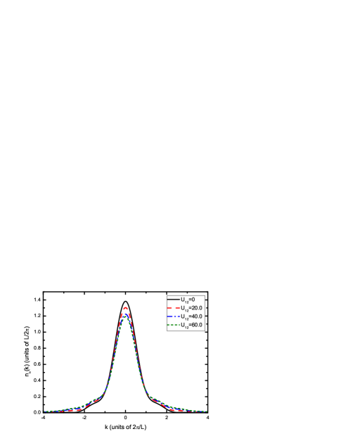
Figure 7: (color online) Momentum distribution of the ground state for $N_{1}=N_{2}=2$, $U_{1}=U_{2}=60.0.$

In Fig. 6 we show the reduced one body density matrix for each component, which means the probability that two successive measurements, one immediately following the other, will find the same component particle at the point $x$ and $x^{\prime}$, respectively. We notice that for all interacting strengthes there exists a strong enhancement of the diagonal contribution $\rho_{\alpha}(x,x^{\prime})$ along the line $x=x^{\prime}$. The identical momentum distributions for the two components are shown in Fig. 7. For all inter-atomic interaction strengths, Bose atoms accumulate in the central regime close to zero momentum and the distributions decrease rapidly for large momentum. For strong inter-component interaction, the momentum distribution becomes broader and broader with the $k=0$ peak diminishing.

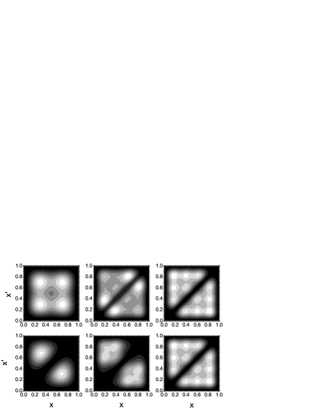
Figure 8: Two-body correlation of intra- and inter-component of the ground state for $N_{1}=N_{2}=2$ and $U_{1}=U_{2}=60.0$. Top: correlation between two atoms in different components; bottom: correlation between two atoms in the same component. $U_{12}=0.0,30.0,60.0$ (from left to right.) Units of length: $L$.

It is also interesting to study the density-density correlation functions, which denote the probability that one measurement will find a atom at the point $x$ and the other one at the point $x^{\prime}$. In Fig. 8 we display the intra- and inter-species correlations between two atoms. At $U_{12}=0.0$ we have two uncorrelated TG gases and thus $\left\langle\hat{\rho}_{1}(x)\hat{\rho}_{2}(x^{\prime})\right\rangle=\left\langle\hat{\rho}_{1}(x)\right\rangle\left\langle\hat{\rho}_{2}(x^{\prime})\right\rangle$. With the increase of the inter-atomic interaction two components will try to avoid each other and it becomes more unlikely that one will find two atoms in different components at the same position. The intra-species correlation is always small in all cases because of the strong intra-atomic interactions in TG limit.

V Summary

In conclusion we have investigated the ground state of two-component Bose gas with Bethe ansatz method and numerical diagonalization method. It turns out that the numerical result describe the ground state of the system quantitatively well. When intra- and inter-atomic interaction are same ($U_{1}=U_{2}=U_{12}$), the two-components Bose gas is integrable and the ground state wavefunction can be obtained exactly. The ground state energy and total density distribution are same for all configurations with same total atom number. With the increase of the interaction the total density distribution show evolution from a Gauss-like Bose distribution (one peak) to a shell structure of nointeracting spinless Fermions ($N$ peaks). The distribution of each component is $N_{\alpha}/N$ of the total density distribution. If the interaction constants deviate the integrable point a little, which is the real situation in experimental, the Bose mixture shows almost same behaviors as the integrable system. In addition we investigate the effect induced by the inter-atomic interaction constants for two TG gases with the numerical diagonalization method. It turns out that with the increase of interspecies interaction the system shows composite fermionization crossover.

Appendix A

The total ground state wave function with $N_{2}$ spin-down particles (the state with $S=N/2$ and $S_{z}=(N_{1}-N_{2})/2$) can be generated by applying the total lowering operator $\hat{S}^{-}=\frac{1}{2}\int dx\hat{\Psi}_{\downarrow}^{\dagger}(x)\hat{\Psi}_{\uparrow}(x)$ to the polarized state according to eq.(7) and its normalized formula shall be expressed as

$$\left|\Psi^{N}\left(\frac{N}{2},\frac{N_{1}-N_{2}}{2}\right)\right\rangle$$

$$= \frac{1}{\sqrt{c}}\int d^{N}\mathbf{x}\Psi\left(x_{1},x_{2},\cdots,x_{N}\right)$$

$$\times\hat{\Psi}_{\downarrow}^{\dagger}(x_{1})\cdots\hat{\Psi}_{\downarrow}^{\dagger}(x_{N_{2}})\hat{\Psi}_{\uparrow}^{\dagger}(x_{N_{2}+1})\cdots\hat{\Psi}_{\uparrow}^{\dagger}(x_{N})\left|0\right\rangle$$

with the normalized constant

$$c = N_{1}!N_{2}!\int dx_{1}\cdots dx_{N}$$

$$\times\Psi\left(x_{1},x_{2},\cdots,x_{N}\right)^{*}\Psi\left(x_{1},x_{2},\cdots,x_{N}\right).$$

The density distribution of $\alpha$th component can be expressed as

$$\rho_{\alpha}(x)=\left\langle\Psi^{N}\left(S,S_{z}\right)\right|\hat{\Psi}_{\alpha}^{\dagger}(x)\hat{\Psi}_{\alpha}(x)\left|\Psi^{N}\left(S,S_{z}\right)\right\rangle$$

$$= \frac{1}{c}\int d^{N}\mathbf{y}d^{N}\mathbf{x}\Psi\left(y_{1},\cdots y_{N}\right)^{*}\Psi\left(x_{1},\cdots x_{N}\right)$$

$$\times\left\langle 0\right|\hat{\Psi}_{\uparrow}(y_{N})\cdots\hat{\Psi}_{\uparrow}(y_{N_{2}+1})\hat{\Psi}_{\downarrow}(y_{N_{2}})\cdots\hat{\Psi}_{\downarrow}(y_{1})\hat{\Psi}_{\alpha}^{\dagger}(x)$$

$$\times\hat{\Psi}_{\alpha}(x)\hat{\Psi}_{\downarrow}^{\dagger}(x_{1})\cdots\hat{\Psi}_{\downarrow}^{\dagger}(x_{N_{2}})\hat{\Psi}_{\uparrow}^{\dagger}(x_{N_{2}+1})\cdots\hat{\Psi}_{\uparrow}^{\dagger}(x_{N})\left|0\right\rangle$$

For the first component the above formulation can be evaluated as follows

$$\rho_{1}(x)=\left\langle\Psi^{N}\left(S,S_{z}\right)\right|\hat{\Psi}_{\uparrow}^{\dagger}(x)\hat{\Psi}_{\uparrow}(x)\left|\Psi^{N}\left(S,S_{z}\right)\right\rangle$$

$$= \frac{1}{c}\int d^{N}\mathbf{y}d^{N}\mathbf{x}\Psi\left(y_{1},\cdots y_{N}\right)^{*}\Psi\left(x_{1},\cdots x_{N}\right)$$

$$\times\left\langle 0\right|\hat{\Psi}_{\uparrow}(y_{N})\cdots\hat{\Psi}_{\uparrow}(y_{N_{2}+1})\hat{\Psi}_{\uparrow}^{\dagger}(x)$$

$$\times\hat{\Psi}_{\uparrow}(x)\hat{\Psi}_{\uparrow}^{\dagger}(x_{N_{2}+1})\cdots\hat{\Psi}_{\uparrow}^{\dagger}(x_{N})$$

$$\times\hat{\Psi}_{\downarrow}(y_{N_{2}})\cdots\hat{\Psi}_{\downarrow}(y_{1})\hat{\Psi}_{\downarrow}^{\dagger}(x_{1})\cdots\hat{\Psi}_{\downarrow}^{\dagger}(x_{N_{2}})\left|0\right\rangle$$

$$= \frac{1}{c}N_{1}N_{1}!N_{2}!\int dx_{2}\cdots dx_{N}$$

$$\times\Psi\left(x,x_{2},\cdots,x_{N}\right)^{*}\Psi\left(x,x_{2},\cdots,x_{N}\right).$$

Similarly, for the second component we have

$$\rho_{2}(x)=\left\langle\Psi^{N}\left(S,S_{z}\right)\right|\hat{\Psi}_{\downarrow}^{\dagger}(x)\hat{\Psi}_{\downarrow}(x)\left|\Psi^{N}\left(S,S_{z}\right)\right\rangle$$

$$= \frac{1}{c}\int d^{N}\mathbf{y}d^{N}\mathbf{x}\Psi\left(y_{1},\cdots y_{N}\right)^{*}\Psi\left(x_{1},\cdots x_{N}\right)$$

$$\times\left\langle 0\right|\hat{\Psi}_{\uparrow}(y_{N})\cdots\hat{\Psi}_{\uparrow}(y_{N_{2}+1})\hat{\Psi}_{\uparrow}^{\dagger}(x_{N_{2}+1})\cdots\hat{\Psi}_{\uparrow}^{\dagger}(x_{N})$$

$$\times\hat{\Psi}_{\downarrow}(y_{N_{2}})\cdots\hat{\Psi}_{\downarrow}(y_{1})\hat{\Psi}_{\downarrow}^{\dagger}(x)\hat{\Psi}_{\downarrow}(x)\hat{\Psi}_{\downarrow}^{\dagger}(x_{1})\cdots\hat{\Psi}_{\downarrow}^{\dagger}(x_{N_{2}})\left|0\right\rangle$$

$$= \frac{1}{c}N_{2}N_{1}!N_{2}!\int dx_{2}\cdots dx_{N}$$

$$\times\Psi\left(x,x_{2},\cdots,x_{N}\right)^{*}\Psi\left(x,x_{2},\cdots,x_{N}\right).$$

Thus the total ground-state density distribution is given by

$$\rho_{\text{tot}}(x)=\rho_{1}(x)+\rho_{2}(x)$$

$$= \frac{N\int dx_{2}\cdots dx_{N}\Psi\left(x,x_{2},\cdots,x_{N}\right)^{*}\Psi\left(x,x_{2},\cdots,x_{N}\right)}{\int dx_{1}\cdots dx_{N}\Psi\left(x_{1},x_{2},\cdots,x_{N}\right)^{*}\Psi\left(x_{1},x_{2},\cdots,x_{N}\right)}$$

with the density distribution of $\alpha$-component

$$\rho_{\alpha}(x)=\frac{N_{\alpha}}{N}\rho_{\text{tot}}(x).$$

References

• (1) C. J. Myatt et al., Phys. Rev. Lett. 78, 586 (1997).
• (2) M. Erhard, H. Schmaljohann, J. Kronjäger, K. Bongs, and K. Sengstock, Phys. Rev. A 69, 032705 (2004); A. Widera, O. Mandel, M. Greiner, S. Kreim, T. W. Hänsch, and I. Bloch, Phys. Rev. Lett. 92, 160406 (2004).
• (3) T.-L. Ho and V. B. Shenoy, Phys. Rev. Lett. 77, 3276 (1996).
• (4) P. Ao and S. T. Chui, Phys. Rev. A 58, 4836 (1998).
• (5) H. Pu and N. P. Bigelow, Phys. Rev. Lett. 80, 1130 (1998).
• (6) M. A. Cazalilla and A. F. Ho, Phys. Rev. Lett. 91, 150403 (2003).
• (7) J. Williams, R. Walser, J. Cooper, E. Cornell and M. Holland, Phys. Rev. A 59, R31 (1999).
• (8) B. D. Esry, Phys. Rev. A 58, R3399 (1998); B. D. Esry and C. H. Greene, Phys. Rev. A 59, 1457 (1999); B. D. Esry, C. H. Greene, J. P. Burke, Jr., and J. L. Bohn, Phys. Rev. Lett. 78, 3594 (1997).
• (9) E. Timmermans, Phys. Rev. Lett. 81, 5718 (1998); S. T. Chui and P. Ao, Phys. Rev. A 59, 1473 (1999).
• (10) T. Stöferle et al., Phys. Rev. Lett. 92, 130403 (2004).
• (11) B. Paredes, A. Widera, V. Murg, O. Mandel, S. Fölling, I. Cirac, G. V. Shlyapnikov, T. W. Hänsch, and I. Bloch, Nature 429, 277 (2004).
• (12) T. Kinoshita, T. Wenger and D. S. Weiss, Science   305, 1125 (2004).
• (13) M. D. Girardeau, J. Math. Phys. (N.Y.) 1, 516 (1960); Phys. Rev. 139, B500 (1965), Secs. 2, 3, and 6.
• (14) M. Olshanii, Phys. Rev. Lett. 81, 938 (1998).
• (15) T. Bergeman, M. G. Moore, and M. Olshanii, Phys. Rev. Lett. 91, 163201 (2003).
• (16) D. S. Petrov, G. V. Shlyapnikov, and J. T. M. Walraven, Phys. Rev. Lett. 85, 3745 (2000).
• (17) V. Dunjko, V. Lorent and M. Olshanii, Phys. Rev. Lett. 86, 5413 (2001).
• (18) S. Chen and R. Egger, Phys. Rev. A. 68, 063605 (2003).
• (19) A. del Campo and J. G. Muga, Europhys. Lett. 74, 965 (2006).
• (20) Y. Hao, Y. Zhang, J. Q. Liang and S. Chen, Phys. Rev. A. 73, 063617 (2006).
• (21) Y. Hao, Y. Zhang, and S. Chen, Phys. Rev. A. 76, 063601 (2007); ibid, 78, 023631 (2008).
• (22) F. Deuretzbacher, K. Bongs, K. Sengstock, and D. Pfannkuche, Phys. Rev. A 75, 013614 (2007).
• (23) S. Zöllner, H.-D. Meyer, and P. Schmelcher, Phys. Rev. A 74, 063611 (2006).
• (24) O. E. Alon, and L. S. Cederbaum, Phys. Rev. Lett. 95, 140402 (2005).
• (25) X. Yin, Y. Hao, S. Chen and Y. Zhang, Phys. Rev. A. 78, 013604 (2008).
• (26) M. D. Girardeau and A. Minguzzi, Phys. Rev. Lett. 99, 230402 (2007).
• (27) F. Deuretzbacher, K. Fredenhagen, D. Becker, K. Bongs, K. Sengstock, and D. Pfannkuche , Phys. Rev. Lett. 100, 160405 (2008).
• (28) L. Guan, S. Chen, Y. Wang and Z. Q. Ma, cond-mat/0806.1773.
• (29) S. Zöllner, H.-D. Meyer, and P. Schmelcher, Phys. Rev. A 78, 013629 (2008).
• (30) Y. J. Hao and S. Chen, Eur. Phys. J. D 51, 261 (2009).
• (31) Y. Q. Li, S. J. Gu, Z. J. Ying and U. Eckern, Europhys. Lett. 61, 368 (2003).
• (32) S. J. Gu, Y. Q. Li, and Z. J. Ying, J. Phys. A 34, 8995 (2001).
• (33) X.-W. Guan, M. T. Batchelor, and M. Takahashi, Phys. Rev. A 76, 043617 (2007); N. Oelkers, M. T. Batchelor, M. Bortz and X.-W. Guan, J. Phys. A 39, 1073 (2006); M. T. Batchelor, M. Bortz, X. W. Guan, and N. Oelkers, Phys. Rev. A 72, 061603 (2005).
• (34) J. N. Fuchs, D. M. Gangardt, T. Keilmann, and G. V. Shlyapnikov, Phys. Rev. Lett. 95, 150402 (2005); M. T. Batchelor, M. Bortz, X. W. Guan, and N. Oelkers, J. Stat. Mech. P03016 (2006).
• (35) E. Eisenberg and E. H. Lieb, Phys. Rev. Lett. 89 , 220403 (2002).
• (36) K. Yang and Y. Q. Li, Int. J. Mod. Phys. B 17, 1027 (2003).
• (37) M. Gaudin, Phys. Rev. A 4, 386 (1971).
• (38) C. N. Yang, Phys. Rev. Lett. 19, 1312 (1967).
• (39) This is true because the conclusion that the ground state for a 2-component boson system with the total SU(2) symmetry is $(N+1)$-foldly degenerate is indepedent of the external potential. Therefore, as long as the total SU(2) symmetry is not broken, one can construct the degenerate states according to Eq. (7). The derivation of Eq. (8) in the appendix does not depend on the concrete form of $\Psi(x_{1},\cdots,x_{N})$ except the property of its exchange symmetry. However when there exists an external potential, for example, a harmonic potential, one can not calculate the wavefunction exactly since the system is no longer integrable.
• (40) M. R. Matthews, D. S. Hall, D. S. Jin, J. R. Ensher, C. E. Wieman, and E. A. Cornell, Phys. Rev. Lett. 81, 243 (1998); J. M. Vogels, C. C. Tsai, R. S. Freeland, S. J. J. M. F. Kokkelmans, B. J. Verhaar, and D. J. Heinzen, Phys. Rev. A 56, R1067 (1997).