CDF Collaboration222With visitors from aUniversity of Massachusetts Amherst, Amherst, Massachusetts 01003,
bUniversiteit Antwerpen, B-2610 Antwerp, Belgium,
cUniversity of Bristol, Bristol BS8 1TL, United Kingdom,
dChinese Academy of Sciences, Beijing 100864, China,
eIstituto Nazionale di Fisica Nucleare, Sezione di Cagliari, 09042 Monserrato (Cagliari), Italy,
fUniversity of California Irvine, Irvine, CA 92697,
gUniversity of California Santa Cruz, Santa Cruz, CA 95064,
hCornell University, Ithaca, NY 14853,
iUniversity of Cyprus, Nicosia CY-1678, Cyprus,
jUniversity College Dublin, Dublin 4, Ireland,
kRoyal Society of Edinburgh/Scottish Executive Support Research Fellow,
lUniversity of Edinburgh, Edinburgh EH9 3JZ, United Kingdom,
mUniversidad Iberoamericana, Mexico D.F., Mexico,
nQueen Mary, University of London, London, E1 4NS, England,
oUniversity of Manchester, Manchester M13 9PL, England,
pNagasaki Institute of Applied Science, Nagasaki, Japan,
qUniversity of Notre Dame, Notre Dame, IN 46556,
rUniversity de Oviedo, E-33007 Oviedo, Spain,
sTexas Tech University, Lubbock, TX 79409,
tIFIC(CSIC-Universitat de Valencia), 46071 Valencia, Spain,
uUniversity of Virginia, Charlottesville, VA 22904,
ccOn leave from J. Stefan Institute, Ljubljana, Slovenia,
Top quark mass measurement in the all hadronic channel using a matrix element technique in collisions at TeV
T. Aaltonen
Division of High Energy Physics, Department of Physics, University of Helsinki and Helsinki Institute of Physics, FIN-00014, Helsinki, Finland
J. Adelman
Enrico Fermi Institute, University of Chicago, Chicago, Illinois 60637
T. Akimoto
University of Tsukuba, Tsukuba, Ibaraki 305, Japan
B. Álvarez González
Instituto de Fisica de Cantabria, CSIC-University of Cantabria, 39005 Santander, Spain
S. AmeriowIstituto Nazionale di Fisica Nucleare, Sezione di Padova-Trento, wUniversity of Padova, I-35131 Padova, Italy
D. Amidei
University of Michigan, Ann Arbor, Michigan 48109
A. Anastassov
Northwestern University, Evanston, Illinois 60208
A. Annovi
Laboratori Nazionali di Frascati, Istituto Nazionale di Fisica Nucleare, I-00044 Frascati, Italy
J. Antos
Comenius University, 842 48 Bratislava, Slovakia; Institute of Experimental Physics, 040 01 Kosice, Slovakia
G. Apollinari
Fermi National Accelerator Laboratory, Batavia, Illinois 60510
A. Apresyan
Purdue University, West Lafayette, Indiana 47907
T. Arisawa
Waseda University, Tokyo 169, Japan
A. Artikov
Joint Institute for Nuclear Research, RU-141980 Dubna, Russia
W. Ashmanskas
Fermi National Accelerator Laboratory, Batavia, Illinois 60510
A. Attal
Institut de Fisica d’Altes Energies, Universitat Autonoma de Barcelona, E-08193, Bellaterra (Barcelona), Spain
A. Aurisano
Texas A&M University, College Station, Texas 77843
F. Azfar
University of Oxford, Oxford OX1 3RH, United Kingdom
P. AzzurrizIstituto Nazionale di Fisica Nucleare Pisa, xUniversity of Pisa, yUniversity of Siena and zScuola Normale Superiore, I-56127 Pisa, Italy
W. Badgett
Fermi National Accelerator Laboratory, Batavia, Illinois 60510
A. Barbaro-Galtieri
Ernest Orlando Lawrence Berkeley National Laboratory, Berkeley, California 94720
V.E. Barnes
Purdue University, West Lafayette, Indiana 47907
B.A. Barnett
The Johns Hopkins University, Baltimore, Maryland 21218
V. Bartsch
University College London, London WC1E 6BT, United Kingdom
G. Bauer
Massachusetts Institute of Technology, Cambridge, Massachusetts 02139
P.-H. Beauchemin
Institute of Particle Physics: McGill University, Montréal, Québec, Canada H3A 2T8; Simon Fraser University, Burnaby, British Columbia, Canada V5A 1S6; University of Toronto, Toronto, Ontario, Canada M5S 1A7; and TRIUMF, Vancouver, British Columbia, Canada V6T 2A3
F. Bedeschi
Istituto Nazionale di Fisica Nucleare Pisa, xUniversity of Pisa, yUniversity of Siena and zScuola Normale Superiore, I-56127 Pisa, Italy
D. Beecher
University College London, London WC1E 6BT, United Kingdom
S. Behari
The Johns Hopkins University, Baltimore, Maryland 21218
G. BellettinixIstituto Nazionale di Fisica Nucleare Pisa, xUniversity of Pisa, yUniversity of Siena and zScuola Normale Superiore, I-56127 Pisa, Italy
J. Bellinger
University of Wisconsin, Madison, Wisconsin 53706
D. Benjamin
Duke University, Durham, North Carolina 27708
A. Beretvas
Fermi National Accelerator Laboratory, Batavia, Illinois 60510
J. Beringer
Ernest Orlando Lawrence Berkeley National Laboratory, Berkeley, California 94720
A. Bhatti
The Rockefeller University, New York, New York 10021
M. Binkley
Fermi National Accelerator Laboratory, Batavia, Illinois 60510
D. BisellowIstituto Nazionale di Fisica Nucleare, Sezione di Padova-Trento, wUniversity of Padova, I-35131 Padova, Italy
I. BizjakccUniversity College London, London WC1E 6BT, United Kingdom
R.E. Blair
Argonne National Laboratory, Argonne, Illinois 60439
C. Blocker
Brandeis University, Waltham, Massachusetts 02254
B. Blumenfeld
The Johns Hopkins University, Baltimore, Maryland 21218
A. Bocci
Duke University, Durham, North Carolina 27708
A. Bodek
University of Rochester, Rochester, New York 14627
V. Boisvert
University of Rochester, Rochester, New York 14627
G. Bolla
Purdue University, West Lafayette, Indiana 47907
D. Bortoletto
Purdue University, West Lafayette, Indiana 47907
J. Boudreau
University of Pittsburgh, Pittsburgh, Pennsylvania 15260
A. Boveia
University of California, Santa Barbara, Santa Barbara, California 93106
B. BrauaUniversity of California, Santa Barbara, Santa Barbara, California 93106
A. Bridgeman
University of Illinois, Urbana, Illinois 61801
L. Brigliadori
Istituto Nazionale di Fisica Nucleare, Sezione di Padova-Trento, wUniversity of Padova, I-35131 Padova, Italy
C. Bromberg
Michigan State University, East Lansing, Michigan 48824
E. Brubaker
Enrico Fermi Institute, University of Chicago, Chicago, Illinois 60637
J. Budagov
Joint Institute for Nuclear Research, RU-141980 Dubna, Russia
H.S. Budd
University of Rochester, Rochester, New York 14627
S. Budd
University of Illinois, Urbana, Illinois 61801
S. Burke
Fermi National Accelerator Laboratory, Batavia, Illinois 60510
K. Burkett
Fermi National Accelerator Laboratory, Batavia, Illinois 60510
G. BusettowIstituto Nazionale di Fisica Nucleare, Sezione di Padova-Trento, wUniversity of Padova, I-35131 Padova, Italy
P. BusseykGlasgow University, Glasgow G12 8QQ, United Kingdom
A. Buzatu
Institute of Particle Physics: McGill University, Montréal, Québec, Canada H3A 2T8; Simon Fraser
University, Burnaby, British Columbia, Canada V5A 1S6; University of Toronto, Toronto, Ontario, Canada M5S 1A7; and TRIUMF, Vancouver, British Columbia, Canada V6T 2A3
K. L. Byrum
Argonne National Laboratory, Argonne, Illinois 60439
S. CabrerauDuke University, Durham, North Carolina 27708
C. Calancha
Centro de Investigaciones Energeticas Medioambientales y Tecnologicas, E-28040 Madrid, Spain
M. Campanelli
Michigan State University, East Lansing, Michigan 48824
M. Campbell
University of Michigan, Ann Arbor, Michigan 48109
F. Canelli14Fermi National Accelerator Laboratory, Batavia, Illinois 60510
A. Canepa
University of Pennsylvania, Philadelphia, Pennsylvania 19104
B. Carls
University of Illinois, Urbana, Illinois 61801
D. Carlsmith
University of Wisconsin, Madison, Wisconsin 53706
R. Carosi
Istituto Nazionale di Fisica Nucleare Pisa, xUniversity of Pisa, yUniversity of Siena and zScuola Normale Superiore, I-56127 Pisa, Italy
S. CarrillomUniversity of Florida, Gainesville, Florida 32611
S. Carron
Institute of Particle Physics: McGill University, Montréal, Québec, Canada H3A 2T8; Simon Fraser University, Burnaby, British Columbia, Canada V5A 1S6; University of Toronto, Toronto, Ontario, Canada M5S 1A7; and TRIUMF, Vancouver, British Columbia, Canada V6T 2A3
B. Casal
Instituto de Fisica de Cantabria, CSIC-University of Cantabria, 39005 Santander, Spain
M. Casarsa
Fermi National Accelerator Laboratory, Batavia, Illinois 60510
A. CastrovIstituto Nazionale di Fisica Nucleare Bologna, vUniversity of Bologna, I-40127 Bologna, Italy
P. CatastiniyIstituto Nazionale di Fisica Nucleare Pisa, xUniversity of Pisa, yUniversity of Siena and zScuola Normale Superiore, I-56127 Pisa, Italy
D. CauzbbIstituto Nazionale di Fisica Nucleare Trieste/Udine, bbUniversity of Trieste/Udine, Italy
V. CavaliereyIstituto Nazionale di Fisica Nucleare Pisa, xUniversity of Pisa, yUniversity of Siena and zScuola Normale Superiore, I-56127 Pisa, Italy
M. Cavalli-Sforza
Institut de Fisica d’Altes Energies, Universitat Autonoma de Barcelona, E-08193, Bellaterra (Barcelona), Spain
A. Cerri
Ernest Orlando Lawrence Berkeley National Laboratory, Berkeley, California 94720
L. CerritonUniversity College London, London WC1E 6BT, United Kingdom
S.H. Chang
Center for High Energy Physics: Kyungpook National University, Daegu 702-701, Korea; Seoul National University, Seoul 151-742, Korea; Sungkyunkwan University, Suwon 440-746, Korea; Korea Institute of Science and Technology Information, Daejeon, 305-806, Korea; Chonnam National University, Gwangju, 500-757, Korea
Y.C. Chen
Institute of Physics, Academia Sinica, Taipei, Taiwan 11529, Republic of China
M. Chertok
University of California, Davis, Davis, California 95616
G. Chiarelli
Istituto Nazionale di Fisica Nucleare Pisa, xUniversity of Pisa, yUniversity of Siena and zScuola Normale Superiore, I-56127 Pisa, Italy
G. Chlachidze
Fermi National Accelerator Laboratory, Batavia, Illinois 60510
F. Chlebana
Fermi National Accelerator Laboratory, Batavia, Illinois 60510
K. Cho
Center for High Energy Physics: Kyungpook National University, Daegu 702-701, Korea; Seoul National University, Seoul 151-742, Korea; Sungkyunkwan University, Suwon 440-746, Korea; Korea Institute of Science and Technology Information, Daejeon, 305-806, Korea; Chonnam National University, Gwangju, 500-757, Korea
D. Chokheli
Joint Institute for Nuclear Research, RU-141980 Dubna, Russia
J.P. Chou
Harvard University, Cambridge, Massachusetts 02138
G. Choudalakis
Massachusetts Institute of Technology, Cambridge, Massachusetts 02139
S.H. Chuang
Rutgers University, Piscataway, New Jersey 08855
K. Chung
Carnegie Mellon University, Pittsburgh, PA 15213
W.H. Chung
University of Wisconsin, Madison, Wisconsin 53706
Y.S. Chung
University of Rochester, Rochester, New York 14627
T. Chwalek
Institut für Experimentelle Kernphysik, Universität Karlsruhe, 76128 Karlsruhe, Germany
C.I. Ciobanu
LPNHE, Universite Pierre et Marie Curie/IN2P3-CNRS, UMR7585, Paris, F-75252 France
M.A. CiocciyIstituto Nazionale di Fisica Nucleare Pisa, xUniversity of Pisa, yUniversity of Siena and zScuola Normale Superiore, I-56127 Pisa, Italy
A. Clark
University of Geneva, CH-1211 Geneva 4, Switzerland
D. Clark
Brandeis University, Waltham, Massachusetts 02254
G. Compostella
Istituto Nazionale di Fisica Nucleare, Sezione di Padova-Trento, wUniversity of Padova, I-35131 Padova, Italy
M.E. Convery
Fermi National Accelerator Laboratory, Batavia, Illinois 60510
J. Conway
University of California, Davis, Davis, California 95616
M. Cordelli
Laboratori Nazionali di Frascati, Istituto Nazionale di Fisica Nucleare, I-00044 Frascati, Italy
G. CortianawIstituto Nazionale di Fisica Nucleare, Sezione di Padova-Trento, wUniversity of Padova, I-35131 Padova, Italy
C.A. Cox
University of California, Davis, Davis, California 95616
D.J. Cox
University of California, Davis, Davis, California 95616
F. CresciolixIstituto Nazionale di Fisica Nucleare Pisa, xUniversity of Pisa, yUniversity of Siena and zScuola Normale Superiore, I-56127 Pisa, Italy
C. Cuenca AlmenaruUniversity of California, Davis, Davis, California 95616
J. CuevasrInstituto de Fisica de Cantabria, CSIC-University of Cantabria, 39005 Santander, Spain
R. Culbertson
Fermi National Accelerator Laboratory, Batavia, Illinois 60510
J.C. Cully
University of Michigan, Ann Arbor, Michigan 48109
D. Dagenhart
Fermi National Accelerator Laboratory, Batavia, Illinois 60510
M. Datta
Fermi National Accelerator Laboratory, Batavia, Illinois 60510
T. Davies
Glasgow University, Glasgow G12 8QQ, United Kingdom
P. de Barbaro
University of Rochester, Rochester, New York 14627
S. De Cecco
Istituto Nazionale di Fisica Nucleare, Sezione di Roma 1, aaSapienza Università di Roma, I-00185 Roma, Italy
A. Deisher
Ernest Orlando Lawrence Berkeley National Laboratory, Berkeley, California 94720
G. De Lorenzo
Institut de Fisica d’Altes Energies, Universitat Autonoma de Barcelona, E-08193, Bellaterra (Barcelona), Spain
M. Dell’OrsoxIstituto Nazionale di Fisica Nucleare Pisa, xUniversity of Pisa, yUniversity of Siena and zScuola Normale Superiore, I-56127 Pisa, Italy
C. Deluca
Institut de Fisica d’Altes Energies, Universitat Autonoma de Barcelona, E-08193, Bellaterra (Barcelona), Spain
L. Demortier
The Rockefeller University, New York, New York 10021
J. Deng
Duke University, Durham, North Carolina 27708
M. Deninno
Istituto Nazionale di Fisica Nucleare Bologna, vUniversity of Bologna, I-40127 Bologna, Italy
P.F. Derwent
Fermi National Accelerator Laboratory, Batavia, Illinois 60510
G.P. di Giovanni
LPNHE, Universite Pierre et Marie Curie/IN2P3-CNRS, UMR7585, Paris, F-75252 France
C. DionisiaaIstituto Nazionale di Fisica Nucleare, Sezione di Roma 1, aaSapienza Università di Roma, I-00185 Roma, Italy
B. Di RuzzabbIstituto Nazionale di Fisica Nucleare Trieste/Udine, bbUniversity of Trieste/Udine, Italy
J.R. Dittmann
Baylor University, Waco, Texas 76798
M. D’Onofrio
Institut de Fisica d’Altes Energies, Universitat Autonoma de Barcelona, E-08193, Bellaterra (Barcelona), Spain
S. DonatixIstituto Nazionale di Fisica Nucleare Pisa, xUniversity of Pisa, yUniversity of Siena and zScuola Normale Superiore, I-56127 Pisa, Italy
P. Dong
University of California, Los Angeles, Los Angeles, California 90024
J. Donini
Istituto Nazionale di Fisica Nucleare, Sezione di Padova-Trento, wUniversity of Padova, I-35131 Padova, Italy
T. Dorigo
Istituto Nazionale di Fisica Nucleare, Sezione di Padova-Trento, wUniversity of Padova, I-35131 Padova, Italy
S. Dube
Rutgers University, Piscataway, New Jersey 08855
J. Efron
The Ohio State University, Columbus, Ohio 43210
A. Elagin
Texas A&M University, College Station, Texas 77843
R. Erbacher
University of California, Davis, Davis, California 95616
D. Errede
University of Illinois, Urbana, Illinois 61801
S. Errede
University of Illinois, Urbana, Illinois 61801
R. Eusebi
Fermi National Accelerator Laboratory, Batavia, Illinois 60510
H.C. Fang
Ernest Orlando Lawrence Berkeley National Laboratory, Berkeley, California 94720
S. Farrington
University of Oxford, Oxford OX1 3RH, United Kingdom
W.T. Fedorko
Enrico Fermi Institute, University of Chicago, Chicago, Illinois 60637
R.G. Feild
Yale University, New Haven, Connecticut 06520
M. Feindt
Institut für Experimentelle Kernphysik, Universität Karlsruhe, 76128 Karlsruhe, Germany
J.P. Fernandez
Centro de Investigaciones Energeticas Medioambientales y Tecnologicas, E-28040 Madrid, Spain
C. FerrazzazIstituto Nazionale di Fisica Nucleare Pisa, xUniversity of Pisa, yUniversity of Siena and zScuola Normale Superiore, I-56127 Pisa, Italy
R. Field
University of Florida, Gainesville, Florida 32611
G. Flanagan
Purdue University, West Lafayette, Indiana 47907
R. Forrest
University of California, Davis, Davis, California 95616
M.J. Frank
Baylor University, Waco, Texas 76798
M. Franklin
Harvard University, Cambridge, Massachusetts 02138
J.C. Freeman
Fermi National Accelerator Laboratory, Batavia, Illinois 60510
I. Furic
University of Florida, Gainesville, Florida 32611
M. Gallinaro
Istituto Nazionale di Fisica Nucleare, Sezione di Roma 1, aaSapienza Università di Roma, I-00185 Roma, Italy
J. Galyardt
Carnegie Mellon University, Pittsburgh, PA 15213
F. Garberson
University of California, Santa Barbara, Santa Barbara, California 93106
J.E. Garcia
University of Geneva, CH-1211 Geneva 4, Switzerland
A.F. Garfinkel
Purdue University, West Lafayette, Indiana 47907
K. Genser
Fermi National Accelerator Laboratory, Batavia, Illinois 60510
H. Gerberich
University of Illinois, Urbana, Illinois 61801
D. Gerdes
University of Michigan, Ann Arbor, Michigan 48109
A. Gessler
Institut für Experimentelle Kernphysik, Universität Karlsruhe, 76128 Karlsruhe, Germany
S. GiaguaaIstituto Nazionale di Fisica Nucleare, Sezione di Roma 1, aaSapienza Università di Roma, I-00185 Roma, Italy
V. Giakoumopoulou
University of Athens, 157 71 Athens, Greece
P. Giannetti
Istituto Nazionale di Fisica Nucleare Pisa, xUniversity of Pisa, yUniversity of Siena and zScuola Normale Superiore, I-56127 Pisa, Italy
K. Gibson
University of Pittsburgh, Pittsburgh, Pennsylvania 15260
J.L. Gimmell
University of Rochester, Rochester, New York 14627
C.M. Ginsburg
Fermi National Accelerator Laboratory, Batavia, Illinois 60510
N. Giokaris
University of Athens, 157 71 Athens, Greece
M. GiordanibbIstituto Nazionale di Fisica Nucleare Trieste/Udine, bbUniversity of Trieste/Udine, Italy
P. Giromini
Laboratori Nazionali di Frascati, Istituto Nazionale di Fisica Nucleare, I-00044 Frascati, Italy
M. GiuntaxIstituto Nazionale di Fisica Nucleare Pisa, xUniversity of Pisa, yUniversity of Siena and zScuola Normale Superiore, I-56127 Pisa, Italy
G. Giurgiu
The Johns Hopkins University, Baltimore, Maryland 21218
V. Glagolev
Joint Institute for Nuclear Research, RU-141980 Dubna, Russia
D. Glenzinski
Fermi National Accelerator Laboratory, Batavia, Illinois 60510
M. Gold
University of New Mexico, Albuquerque, New Mexico 87131
N. Goldschmidt
University of Florida, Gainesville, Florida 32611
A. Golossanov
Fermi National Accelerator Laboratory, Batavia, Illinois 60510
G. Gomez
Instituto de Fisica de Cantabria, CSIC-University of Cantabria, 39005 Santander, Spain
G. Gomez-Ceballos
Massachusetts Institute of Technology, Cambridge, Massachusetts 02139
M. Goncharov
Massachusetts Institute of Technology, Cambridge, Massachusetts 02139
O. González
Centro de Investigaciones Energeticas Medioambientales y Tecnologicas, E-28040 Madrid, Spain
I. Gorelov
University of New Mexico, Albuquerque, New Mexico 87131
A.T. Goshaw
Duke University, Durham, North Carolina 27708
K. Goulianos
The Rockefeller University, New York, New York 10021
A. GreselewIstituto Nazionale di Fisica Nucleare, Sezione di Padova-Trento, wUniversity of Padova, I-35131 Padova, Italy
S. Grinstein
Harvard University, Cambridge, Massachusetts 02138
C. Grosso-Pilcher
Enrico Fermi Institute, University of Chicago, Chicago, Illinois 60637
R.C. Group
Fermi National Accelerator Laboratory, Batavia, Illinois 60510
U. Grundler
University of Illinois, Urbana, Illinois 61801
J. Guimaraes da Costa
Harvard University, Cambridge, Massachusetts 02138
Z. Gunay-Unalan
Michigan State University, East Lansing, Michigan 48824
C. Haber
Ernest Orlando Lawrence Berkeley National Laboratory, Berkeley, California 94720
K. Hahn
Massachusetts Institute of Technology, Cambridge, Massachusetts 02139
S.R. Hahn
Fermi National Accelerator Laboratory, Batavia, Illinois 60510
E. Halkiadakis
Rutgers University, Piscataway, New Jersey 08855
B.-Y. Han
University of Rochester, Rochester, New York 14627
J.Y. Han
University of Rochester, Rochester, New York 14627
F. Happacher
Laboratori Nazionali di Frascati, Istituto Nazionale di Fisica Nucleare, I-00044 Frascati, Italy
K. Hara
University of Tsukuba, Tsukuba, Ibaraki 305, Japan
D. Hare
Rutgers University, Piscataway, New Jersey 08855
M. Hare
Tufts University, Medford, Massachusetts 02155
S. Harper
University of Oxford, Oxford OX1 3RH, United Kingdom
R.F. Harr
Wayne State University, Detroit, Michigan 48201
R.M. Harris
Fermi National Accelerator Laboratory, Batavia, Illinois 60510
M. Hartz
University of Pittsburgh, Pittsburgh, Pennsylvania 15260
K. Hatakeyama
The Rockefeller University, New York, New York 10021
C. Hays
University of Oxford, Oxford OX1 3RH, United Kingdom
M. Heck
Institut für Experimentelle Kernphysik, Universität Karlsruhe, 76128 Karlsruhe, Germany
A. Heijboer
University of Pennsylvania, Philadelphia, Pennsylvania 19104
J. Heinrich
University of Pennsylvania, Philadelphia, Pennsylvania 19104
C. Henderson
Massachusetts Institute of Technology, Cambridge, Massachusetts 02139
M. Herndon
University of Wisconsin, Madison, Wisconsin 53706
J. Heuser
Institut für Experimentelle Kernphysik, Universität Karlsruhe, 76128 Karlsruhe, Germany
S. Hewamanage
Baylor University, Waco, Texas 76798
D. Hidas
Duke University, Durham, North Carolina 27708
C.S. HillcUniversity of California, Santa Barbara, Santa Barbara, California 93106
D. Hirschbuehl
Institut für Experimentelle Kernphysik, Universität Karlsruhe, 76128 Karlsruhe, Germany
A. Hocker
Fermi National Accelerator Laboratory, Batavia, Illinois 60510
S. Hou
Institute of Physics, Academia Sinica, Taipei, Taiwan 11529, Republic of China
M. Houlden
University of Liverpool, Liverpool L69 7ZE, United Kingdom
S.-C. Hsu
Ernest Orlando Lawrence Berkeley National Laboratory, Berkeley, California 94720
B.T. Huffman
University of Oxford, Oxford OX1 3RH, United Kingdom
R.E. Hughes
The Ohio State University, Columbus, Ohio 43210
U. Husemann
M. Hussein
Michigan State University, East Lansing, Michigan 48824
U. Husemann
Yale University, New Haven, Connecticut 06520
J. Huston
Michigan State University, East Lansing, Michigan 48824
J. Incandela
University of California, Santa Barbara, Santa Barbara, California 93106
G. Introzzi
Istituto Nazionale di Fisica Nucleare Pisa, xUniversity of Pisa, yUniversity of Siena and zScuola Normale Superiore, I-56127 Pisa, Italy
M. IoriaaIstituto Nazionale di Fisica Nucleare, Sezione di Roma 1, aaSapienza Università di Roma, I-00185 Roma, Italy
A. Ivanov
University of California, Davis, Davis, California 95616
E. James
Fermi National Accelerator Laboratory, Batavia, Illinois 60510
B. Jayatilaka
Duke University, Durham, North Carolina 27708
E.J. Jeon
Center for High Energy Physics: Kyungpook National University, Daegu 702-701, Korea; Seoul National University, Seoul 151-742, Korea; Sungkyunkwan University, Suwon 440-746, Korea; Korea Institute of Science and Technology Information, Daejeon, 305-806, Korea; Chonnam National University, Gwangju, 500-757, Korea
M.K. Jha
Istituto Nazionale di Fisica Nucleare Bologna, vUniversity of Bologna, I-40127 Bologna, Italy
S. Jindariani
Fermi National Accelerator Laboratory, Batavia, Illinois 60510
W. Johnson
University of California, Davis, Davis, California 95616
M. Jones
Purdue University, West Lafayette, Indiana 47907
K.K. Joo
Center for High Energy Physics: Kyungpook National University, Daegu 702-701, Korea; Seoul National University, Seoul 151-742, Korea; Sungkyunkwan University, Suwon 440-746, Korea; Korea Institute of Science and Technology Information, Daejeon, 305-806, Korea; Chonnam National University, Gwangju, 500-757, Korea
S.Y. Jun
Carnegie Mellon University, Pittsburgh, PA 15213
J.E. Jung
Center for High Energy Physics: Kyungpook National University, Daegu 702-701, Korea; Seoul National University, Seoul 151-742, Korea; Sungkyunkwan University, Suwon 440-746, Korea; Korea Institute of Science and Technology Information, Daejeon, 305-806, Korea; Chonnam National University, Gwangju, 500-757, Korea
T.R. Junk
Fermi National Accelerator Laboratory, Batavia, Illinois 60510
T. Kamon
Texas A&M University, College Station, Texas 77843
D. Kar
University of Florida, Gainesville, Florida 32611
P.E. Karchin
Wayne State University, Detroit, Michigan 48201
Y. Kato
Osaka City University, Osaka 588, Japan
R. Kephart
Fermi National Accelerator Laboratory, Batavia, Illinois 60510
J. Keung
University of Pennsylvania, Philadelphia, Pennsylvania 19104
V. Khotilovich
Texas A&M University, College Station, Texas 77843
B. Kilminster
Fermi National Accelerator Laboratory, Batavia, Illinois 60510
D.H. Kim
Center for High Energy Physics: Kyungpook National University, Daegu 702-701, Korea; Seoul National University, Seoul 151-742, Korea; Sungkyunkwan University, Suwon 440-746, Korea; Korea Institute of Science and Technology Information, Daejeon, 305-806, Korea; Chonnam National University, Gwangju, 500-757, Korea
H.S. Kim
Center for High Energy Physics: Kyungpook National University, Daegu 702-701, Korea; Seoul National University, Seoul 151-742, Korea; Sungkyunkwan University, Suwon 440-746, Korea; Korea Institute of Science and Technology Information, Daejeon, 305-806, Korea; Chonnam National University, Gwangju, 500-757, Korea
H.W. Kim
Center for High Energy Physics: Kyungpook National University, Daegu 702-701, Korea; Seoul National University, Seoul 151-742, Korea; Sungkyunkwan University, Suwon 440-746, Korea; Korea Institute of Science and Technology Information, Daejeon, 305-806, Korea; Chonnam National University, Gwangju, 500-757, Korea
J.E. Kim
Center for High Energy Physics: Kyungpook National University, Daegu 702-701, Korea; Seoul National University, Seoul 151-742, Korea; Sungkyunkwan University, Suwon 440-746, Korea; Korea Institute of Science and Technology Information, Daejeon, 305-806, Korea; Chonnam National University, Gwangju, 500-757, Korea
M.J. Kim
Laboratori Nazionali di Frascati, Istituto Nazionale di Fisica Nucleare, I-00044 Frascati, Italy
S.B. Kim
Center for High Energy Physics: Kyungpook National University, Daegu 702-701, Korea; Seoul National University, Seoul 151-742, Korea; Sungkyunkwan University, Suwon 440-746, Korea; Korea Institute of Science and Technology Information, Daejeon, 305-806, Korea; Chonnam National University, Gwangju, 500-757, Korea
S.H. Kim
University of Tsukuba, Tsukuba, Ibaraki 305, Japan
Y.K. Kim
Enrico Fermi Institute, University of Chicago, Chicago, Illinois 60637
N. Kimura
University of Tsukuba, Tsukuba, Ibaraki 305, Japan
L. Kirsch
Brandeis University, Waltham, Massachusetts 02254
S. Klimenko
University of Florida, Gainesville, Florida 32611
B. Knuteson
Massachusetts Institute of Technology, Cambridge, Massachusetts 02139
B.R. Ko
Duke University, Durham, North Carolina 27708
K. Kondo
Waseda University, Tokyo 169, Japan
D.J. Kong
Center for High Energy Physics: Kyungpook National University, Daegu 702-701, Korea; Seoul National University, Seoul 151-742, Korea; Sungkyunkwan University, Suwon 440-746, Korea; Korea Institute of Science and Technology Information, Daejeon, 305-806, Korea; Chonnam National University, Gwangju, 500-757, Korea
J. Konigsberg
University of Florida, Gainesville, Florida 32611
A. Korytov
University of Florida, Gainesville, Florida 32611
A.V. Kotwal
Duke University, Durham, North Carolina 27708
M. Kreps
Institut für Experimentelle Kernphysik, Universität Karlsruhe, 76128 Karlsruhe, Germany
J. Kroll
University of Pennsylvania, Philadelphia, Pennsylvania 19104
D. Krop
Enrico Fermi Institute, University of Chicago, Chicago, Illinois 60637
N. Krumnack
Baylor University, Waco, Texas 76798
M. Kruse
Duke University, Durham, North Carolina 27708
V. Krutelyov
University of California, Santa Barbara, Santa Barbara, California 93106
T. Kubo
University of Tsukuba, Tsukuba, Ibaraki 305, Japan
T. Kuhr
Institut für Experimentelle Kernphysik, Universität Karlsruhe, 76128 Karlsruhe, Germany
N.P. Kulkarni
Wayne State University, Detroit, Michigan 48201
M. Kurata
University of Tsukuba, Tsukuba, Ibaraki 305, Japan
S. Kwang
Enrico Fermi Institute, University of Chicago, Chicago, Illinois 60637
A.T. Laasanen
Purdue University, West Lafayette, Indiana 47907
S. Lami
Istituto Nazionale di Fisica Nucleare Pisa, xUniversity of Pisa, yUniversity of Siena and zScuola Normale Superiore, I-56127 Pisa, Italy
S. Lammel
Fermi National Accelerator Laboratory, Batavia, Illinois 60510
M. Lancaster
University College London, London WC1E 6BT, United Kingdom
R.L. Lander
University of California, Davis, Davis, California 95616
K. LannonqThe Ohio State University, Columbus, Ohio 43210
A. Lath
Rutgers University, Piscataway, New Jersey 08855
G. LatinoyIstituto Nazionale di Fisica Nucleare Pisa, xUniversity of Pisa, yUniversity of Siena and zScuola Normale Superiore, I-56127 Pisa, Italy
I. LazzizzerawIstituto Nazionale di Fisica Nucleare, Sezione di Padova-Trento, wUniversity of Padova, I-35131 Padova, Italy
T. LeCompte
Argonne National Laboratory, Argonne, Illinois 60439
E. Lee
Texas A&M University, College Station, Texas 77843
H.S. Lee
Enrico Fermi Institute, University of Chicago, Chicago, Illinois 60637
S.W. LeetTexas A&M University, College Station, Texas 77843
S. Leone
Istituto Nazionale di Fisica Nucleare Pisa, xUniversity of Pisa, yUniversity of Siena and zScuola Normale Superiore, I-56127 Pisa, Italy
J.D. Lewis
Fermi National Accelerator Laboratory, Batavia, Illinois 60510
C.-S. Lin
Ernest Orlando Lawrence Berkeley National Laboratory, Berkeley, California 94720
J. Linacre
University of Oxford, Oxford OX1 3RH, United Kingdom
M. Lindgren
Fermi National Accelerator Laboratory, Batavia, Illinois 60510
E. Lipeles
University of Pennsylvania, Philadelphia, Pennsylvania 19104
A. Lister
University of California, Davis, Davis, California 95616
D.O. Litvintsev
Fermi National Accelerator Laboratory, Batavia, Illinois 60510
C. Liu
University of Pittsburgh, Pittsburgh, Pennsylvania 15260
T. Liu
Fermi National Accelerator Laboratory, Batavia, Illinois 60510
N.S. Lockyer
University of Pennsylvania, Philadelphia, Pennsylvania 19104
A. Loginov
Yale University, New Haven, Connecticut 06520
M. LoretiwIstituto Nazionale di Fisica Nucleare, Sezione di Padova-Trento, wUniversity of Padova, I-35131 Padova, Italy
L. Lovas
Comenius University, 842 48 Bratislava, Slovakia; Institute of Experimental Physics, 040 01 Kosice, Slovakia
D. LucchesiwIstituto Nazionale di Fisica Nucleare, Sezione di Padova-Trento, wUniversity of Padova, I-35131 Padova, Italy
C. LuciaaIstituto Nazionale di Fisica Nucleare, Sezione di Roma 1, aaSapienza Università di Roma, I-00185 Roma, Italy
J. Lueck
Institut für Experimentelle Kernphysik, Universität Karlsruhe, 76128 Karlsruhe, Germany
P. Lujan
Ernest Orlando Lawrence Berkeley National Laboratory, Berkeley, California 94720
P. Lukens
Fermi National Accelerator Laboratory, Batavia, Illinois 60510
G. Lungu
The Rockefeller University, New York, New York 10021
L. Lyons
University of Oxford, Oxford OX1 3RH, United Kingdom
J. Lys
Ernest Orlando Lawrence Berkeley National Laboratory, Berkeley, California 94720
R. Lysak
Comenius University, 842 48 Bratislava, Slovakia; Institute of Experimental Physics, 040 01 Kosice, Slovakia
D. MacQueen
Institute of Particle Physics: McGill University, Montréal, Québec, Canada H3A 2T8; Simon
Fraser University, Burnaby, British Columbia, Canada V5A 1S6; University of Toronto, Toronto, Ontario, Canada M5S 1A7; and TRIUMF, Vancouver, British Columbia, Canada V6T 2A3
R. Madrak
Fermi National Accelerator Laboratory, Batavia, Illinois 60510
K. Maeshima
Fermi National Accelerator Laboratory, Batavia, Illinois 60510
K. Makhoul
Massachusetts Institute of Technology, Cambridge, Massachusetts 02139
T. Maki
Division of High Energy Physics, Department of Physics, University of Helsinki and Helsinki Institute of Physics, FIN-00014, Helsinki, Finland
P. Maksimovic
The Johns Hopkins University, Baltimore, Maryland 21218
S. Malde
University of Oxford, Oxford OX1 3RH, United Kingdom
S. Malik
University College London, London WC1E 6BT, United Kingdom
G. MancaeUniversity of Liverpool, Liverpool L69 7ZE, United Kingdom
A. Manousakis-Katsikakis
University of Athens, 157 71 Athens, Greece
F. Margaroli
Purdue University, West Lafayette, Indiana 47907
C. Marino
Institut für Experimentelle Kernphysik, Universität Karlsruhe, 76128 Karlsruhe, Germany
C.P. Marino
University of Illinois, Urbana, Illinois 61801
A. Martin
Yale University, New Haven, Connecticut 06520
V. MartinlGlasgow University, Glasgow G12 8QQ, United Kingdom
M. Martínez
Institut de Fisica d’Altes Energies, Universitat Autonoma de Barcelona, E-08193, Bellaterra (Barcelona), Spain
R. Martínez-Ballarín
Centro de Investigaciones Energeticas Medioambientales y Tecnologicas, E-28040 Madrid, Spain
T. Maruyama
University of Tsukuba, Tsukuba, Ibaraki 305, Japan
P. Mastrandrea
Istituto Nazionale di Fisica Nucleare, Sezione di Roma 1, aaSapienza Università di Roma, I-00185 Roma, Italy
T. Masubuchi
University of Tsukuba, Tsukuba, Ibaraki 305, Japan
M. Mathis
The Johns Hopkins University, Baltimore, Maryland 21218
M.E. Mattson
Wayne State University, Detroit, Michigan 48201
P. Mazzanti
Istituto Nazionale di Fisica Nucleare Bologna, vUniversity of Bologna, I-40127 Bologna, Italy
K.S. McFarland
University of Rochester, Rochester, New York 14627
P. McIntyre
Texas A&M University, College Station, Texas 77843
R. McNultyjUniversity of Liverpool, Liverpool L69 7ZE, United Kingdom
A. Mehta
University of Liverpool, Liverpool L69 7ZE, United Kingdom
P. Mehtala
Division of High Energy Physics, Department of Physics, University of Helsinki and Helsinki Institute of Physics, FIN-00014, Helsinki, Finland
A. Menzione
Istituto Nazionale di Fisica Nucleare Pisa, xUniversity of Pisa, yUniversity of Siena and zScuola Normale Superiore, I-56127 Pisa, Italy
P. Merkel
Purdue University, West Lafayette, Indiana 47907
C. Mesropian
The Rockefeller University, New York, New York 10021
T. Miao
Fermi National Accelerator Laboratory, Batavia, Illinois 60510
N. Miladinovic
Brandeis University, Waltham, Massachusetts 02254
R. Miller
Michigan State University, East Lansing, Michigan 48824
C. Mills
Harvard University, Cambridge, Massachusetts 02138
M. Milnik
Institut für Experimentelle Kernphysik, Universität Karlsruhe, 76128 Karlsruhe, Germany
A. Mitra
Institute of Physics, Academia Sinica, Taipei, Taiwan 11529, Republic of China
G. Mitselmakher
University of Florida, Gainesville, Florida 32611
H. Miyake
University of Tsukuba, Tsukuba, Ibaraki 305, Japan
N. Moggi
Istituto Nazionale di Fisica Nucleare Bologna, vUniversity of Bologna, I-40127 Bologna, Italy
C.S. Moon
Center for High Energy Physics: Kyungpook National University, Daegu 702-701, Korea; Seoul National University, Seoul 151-742, Korea; Sungkyunkwan University, Suwon 440-746, Korea; Korea Institute of Science and Technology Information, Daejeon, 305-806, Korea; Chonnam National University, Gwangju, 500-757, Korea
R. Moore
Fermi National Accelerator Laboratory, Batavia, Illinois 60510
M.J. MorelloxIstituto Nazionale di Fisica Nucleare Pisa, xUniversity of Pisa, yUniversity of Siena and zScuola Normale Superiore, I-56127 Pisa, Italy
J. Morlok
Institut für Experimentelle Kernphysik, Universität Karlsruhe, 76128 Karlsruhe, Germany
P. Movilla Fernandez
Fermi National Accelerator Laboratory, Batavia, Illinois 60510
J. Mülmenstädt
Ernest Orlando Lawrence Berkeley National Laboratory, Berkeley, California 94720
A. Mukherjee
Fermi National Accelerator Laboratory, Batavia, Illinois 60510
Th. Muller
Institut für Experimentelle Kernphysik, Universität Karlsruhe, 76128 Karlsruhe, Germany
R. Mumford
The Johns Hopkins University, Baltimore, Maryland 21218
P. Murat
Fermi National Accelerator Laboratory, Batavia, Illinois 60510
M. MussinivIstituto Nazionale di Fisica Nucleare Bologna, vUniversity of Bologna, I-40127 Bologna, Italy
J. Nachtman
Fermi National Accelerator Laboratory, Batavia, Illinois 60510
Y. Nagai
University of Tsukuba, Tsukuba, Ibaraki 305, Japan
A. Nagano
University of Tsukuba, Tsukuba, Ibaraki 305, Japan
J. Naganoma
University of Tsukuba, Tsukuba, Ibaraki 305, Japan
K. Nakamura
University of Tsukuba, Tsukuba, Ibaraki 305, Japan
I. Nakano
Okayama University, Okayama 700-8530, Japan
A. Napier
Tufts University, Medford, Massachusetts 02155
V. Necula
Duke University, Durham, North Carolina 27708
J. Nett
University of Wisconsin, Madison, Wisconsin 53706
C. NeuvUniversity of Pennsylvania, Philadelphia, Pennsylvania 19104
M.S. Neubauer
University of Illinois, Urbana, Illinois 61801
S. Neubauer
Institut für Experimentelle Kernphysik, Universität Karlsruhe, 76128 Karlsruhe, Germany
J. NielsengErnest Orlando Lawrence Berkeley National Laboratory, Berkeley, California 94720
L. Nodulman
Argonne National Laboratory, Argonne, Illinois 60439
M. Norman
University of California, San Diego, La Jolla, California 92093
O. Norniella
University of Illinois, Urbana, Illinois 61801
E. Nurse
University College London, London WC1E 6BT, United Kingdom
L. Oakes
University of Oxford, Oxford OX1 3RH, United Kingdom
S.H. Oh
Duke University, Durham, North Carolina 27708
Y.D. Oh
Center for High Energy Physics: Kyungpook National University, Daegu 702-701, Korea; Seoul National University, Seoul 151-742, Korea; Sungkyunkwan University, Suwon 440-746, Korea; Korea Institute of Science and Technology Information, Daejeon, 305-806, Korea; Chonnam National University, Gwangju, 500-757, Korea
I. Oksuzian
University of Florida, Gainesville, Florida 32611
T. Okusawa
Osaka City University, Osaka 588, Japan
R. Orava
Division of High Energy Physics, Department of Physics, University of Helsinki and Helsinki Institute of Physics, FIN-00014, Helsinki, Finland
S. Pagan GrisowIstituto Nazionale di Fisica Nucleare, Sezione di Padova-Trento, wUniversity of Padova, I-35131 Padova, Italy
E. Palencia
Fermi National Accelerator Laboratory, Batavia, Illinois 60510
V. Papadimitriou
Fermi National Accelerator Laboratory, Batavia, Illinois 60510
A. Papaikonomou
Institut für Experimentelle Kernphysik, Universität Karlsruhe, 76128 Karlsruhe, Germany
A.A. Paramonov
Enrico Fermi Institute, University of Chicago, Chicago, Illinois 60637
B. Parks
The Ohio State University, Columbus, Ohio 43210
S. Pashapour
Institute of Particle Physics: McGill University, Montréal, Québec, Canada H3A 2T8; Simon Fraser University, Burnaby, British Columbia, Canada V5A 1S6; University of Toronto, Toronto, Ontario, Canada M5S 1A7; and TRIUMF, Vancouver, British Columbia, Canada V6T 2A3
J. Patrick
Fermi National Accelerator Laboratory, Batavia, Illinois 60510
G. PaulettabbIstituto Nazionale di Fisica Nucleare Trieste/Udine, bbUniversity of Trieste/Udine, Italy
M. Paulini
Carnegie Mellon University, Pittsburgh, PA 15213
C. Paus
Massachusetts Institute of Technology, Cambridge, Massachusetts 02139
T. Peiffer
Institut für Experimentelle Kernphysik, Universität Karlsruhe, 76128 Karlsruhe, Germany
D.E. Pellett
University of California, Davis, Davis, California 95616
A. Penzo
Istituto Nazionale di Fisica Nucleare Trieste/Udine, bbUniversity of Trieste/Udine, Italy
T.J. Phillips
Duke University, Durham, North Carolina 27708
G. Piacentino
Istituto Nazionale di Fisica Nucleare Pisa, xUniversity of Pisa, yUniversity of Siena and zScuola Normale Superiore, I-56127 Pisa, Italy
E. Pianori
University of Pennsylvania, Philadelphia, Pennsylvania 19104
L. Pinera
University of Florida, Gainesville, Florida 32611
K. Pitts
University of Illinois, Urbana, Illinois 61801
C. Plager
University of California, Los Angeles, Los Angeles, California 90024
L. Pondrom
University of Wisconsin, Madison, Wisconsin 53706
O. Poukhov111DeceasedJoint Institute for Nuclear Research, RU-141980 Dubna, Russia
N. Pounder
University of Oxford, Oxford OX1 3RH, United Kingdom
F. Prakoshyn
Joint Institute for Nuclear Research, RU-141980 Dubna, Russia
A. Pronko
Fermi National Accelerator Laboratory, Batavia, Illinois 60510
J. Proudfoot
Argonne National Laboratory, Argonne, Illinois 60439
F. PtohosiFermi National Accelerator Laboratory, Batavia, Illinois 60510
E. Pueschel
Carnegie Mellon University, Pittsburgh, PA 15213
G. PunzixIstituto Nazionale di Fisica Nucleare Pisa, xUniversity of Pisa, yUniversity of Siena and zScuola Normale Superiore, I-56127 Pisa, Italy
J. Pursley
University of Wisconsin, Madison, Wisconsin 53706
J. RademackercUniversity of Oxford, Oxford OX1 3RH, United Kingdom
A. Rahaman
University of Pittsburgh, Pittsburgh, Pennsylvania 15260
V. Ramakrishnan
University of Wisconsin, Madison, Wisconsin 53706
N. Ranjan
Purdue University, West Lafayette, Indiana 47907
I. Redondo
Centro de Investigaciones Energeticas Medioambientales y Tecnologicas, E-28040 Madrid, Spain
P. Renton
University of Oxford, Oxford OX1 3RH, United Kingdom
M. Renz
Institut für Experimentelle Kernphysik, Universität Karlsruhe, 76128 Karlsruhe, Germany
M. Rescigno
Istituto Nazionale di Fisica Nucleare, Sezione di Roma 1, aaSapienza Università di Roma, I-00185 Roma, Italy
S. Richter
Institut für Experimentelle Kernphysik, Universität Karlsruhe, 76128 Karlsruhe, Germany
F. RimondivIstituto Nazionale di Fisica Nucleare Bologna, vUniversity of Bologna, I-40127 Bologna, Italy
L. Ristori
Istituto Nazionale di Fisica Nucleare Pisa, xUniversity of Pisa, yUniversity of Siena and zScuola Normale Superiore, I-56127 Pisa, Italy
A. Robson
Glasgow University, Glasgow G12 8QQ, United Kingdom
T. Rodrigo
Instituto de Fisica de Cantabria, CSIC-University of Cantabria, 39005 Santander, Spain
T. Rodriguez
University of Pennsylvania, Philadelphia, Pennsylvania 19104
E. Rogers
University of Illinois, Urbana, Illinois 61801
S. Rolli
Tufts University, Medford, Massachusetts 02155
R. Roser
Fermi National Accelerator Laboratory, Batavia, Illinois 60510
M. Rossi
Istituto Nazionale di Fisica Nucleare Trieste/Udine, bbUniversity of Trieste/Udine, Italy
R. Rossin
University of California, Santa Barbara, Santa Barbara, California 93106
P. Roy
Institute of Particle Physics: McGill University, Montréal, Québec, Canada H3A 2T8; Simon
Fraser University, Burnaby, British Columbia, Canada V5A 1S6; University of Toronto, Toronto, Ontario, Canada
M5S 1A7; and TRIUMF, Vancouver, British Columbia, Canada V6T 2A3
A. Ruiz
Instituto de Fisica de Cantabria, CSIC-University of Cantabria, 39005 Santander, Spain
J. Russ
Carnegie Mellon University, Pittsburgh, PA 15213
V. Rusu
Fermi National Accelerator Laboratory, Batavia, Illinois 60510
A. Safonov
Texas A&M University, College Station, Texas 77843
W.K. Sakumoto
University of Rochester, Rochester, New York 14627
O. Saltó
Institut de Fisica d’Altes Energies, Universitat Autonoma de Barcelona, E-08193, Bellaterra (Barcelona), Spain
L. SantibbIstituto Nazionale di Fisica Nucleare Trieste/Udine, bbUniversity of Trieste/Udine, Italy
S. SarkaraaIstituto Nazionale di Fisica Nucleare, Sezione di Roma 1, aaSapienza Università di Roma, I-00185 Roma, Italy
L. Sartori
Istituto Nazionale di Fisica Nucleare Pisa, xUniversity of Pisa, yUniversity of Siena and zScuola Normale Superiore, I-56127 Pisa, Italy
K. Sato
Fermi National Accelerator Laboratory, Batavia, Illinois 60510
A. Savoy-Navarro
LPNHE, Universite Pierre et Marie Curie/IN2P3-CNRS, UMR7585, Paris, F-75252 France
P. Schlabach
Fermi National Accelerator Laboratory, Batavia, Illinois 60510
A. Schmidt
Institut für Experimentelle Kernphysik, Universität Karlsruhe, 76128 Karlsruhe, Germany
E.E. Schmidt
Fermi National Accelerator Laboratory, Batavia, Illinois 60510
M.A. Schmidt
Enrico Fermi Institute, University of Chicago, Chicago, Illinois 60637
M.P. Schmidt††footnotemark: Yale University, New Haven, Connecticut 06520
M. Schmitt
Northwestern University, Evanston, Illinois 60208
T. Schwarz
University of California, Davis, Davis, California 95616
L. Scodellaro
Instituto de Fisica de Cantabria, CSIC-University of Cantabria, 39005 Santander, Spain
A. ScribanoyIstituto Nazionale di Fisica Nucleare Pisa, xUniversity of Pisa, yUniversity of Siena and zScuola Normale Superiore, I-56127 Pisa, Italy
F. Scuri
Istituto Nazionale di Fisica Nucleare Pisa, xUniversity of Pisa, yUniversity of Siena and zScuola Normale Superiore, I-56127 Pisa, Italy
A. Sedov
Purdue University, West Lafayette, Indiana 47907
S. Seidel
University of New Mexico, Albuquerque, New Mexico 87131
Y. Seiya
Osaka City University, Osaka 588, Japan
A. Semenov
Joint Institute for Nuclear Research, RU-141980 Dubna, Russia
L. Sexton-Kennedy
Fermi National Accelerator Laboratory, Batavia, Illinois 60510
F. Sforza
Istituto Nazionale di Fisica Nucleare Pisa, xUniversity of Pisa, yUniversity of Siena and zScuola Normale Superiore, I-56127 Pisa, Italy
A. Sfyrla
University of Illinois, Urbana, Illinois 61801
S.Z. Shalhout
Wayne State University, Detroit, Michigan 48201
T. Shears
University of Liverpool, Liverpool L69 7ZE, United Kingdom
P.F. Shepard
University of Pittsburgh, Pittsburgh, Pennsylvania 15260
M. ShimojimapUniversity of Tsukuba, Tsukuba, Ibaraki 305, Japan
S. Shiraishi
Enrico Fermi Institute, University of Chicago, Chicago, Illinois 60637
M. Shochet
Enrico Fermi Institute, University of Chicago, Chicago, Illinois 60637
Y. Shon
University of Wisconsin, Madison, Wisconsin 53706
I. Shreyber
Institution for Theoretical and Experimental Physics, ITEP, Moscow 117259, Russia
A. Sidoti
Istituto Nazionale di Fisica Nucleare Pisa, xUniversity of Pisa, yUniversity of Siena and zScuola Normale Superiore, I-56127 Pisa, Italy
P. Sinervo
Institute of Particle Physics: McGill University, Montréal, Québec, Canada H3A 2T8; Simon Fraser University, Burnaby, British Columbia, Canada V5A 1S6; University of Toronto, Toronto, Ontario, Canada M5S 1A7; and TRIUMF, Vancouver, British Columbia, Canada V6T 2A3
A. Sisakyan
Joint Institute for Nuclear Research, RU-141980 Dubna, Russia
A.J. Slaughter
Fermi National Accelerator Laboratory, Batavia, Illinois 60510
J. Slaunwhite
The Ohio State University, Columbus, Ohio 43210
K. Sliwa
Tufts University, Medford, Massachusetts 02155
J.R. Smith
University of California, Davis, Davis, California 95616
F.D. Snider
Fermi National Accelerator Laboratory, Batavia, Illinois 60510
R. Snihur
Institute of Particle Physics: McGill University, Montréal, Québec, Canada H3A 2T8; Simon
Fraser University, Burnaby, British Columbia, Canada V5A 1S6; University of Toronto, Toronto, Ontario, Canada
M5S 1A7; and TRIUMF, Vancouver, British Columbia, Canada V6T 2A3
A. Soha
University of California, Davis, Davis, California 95616
S. Somalwar
Rutgers University, Piscataway, New Jersey 08855
V. Sorin
Michigan State University, East Lansing, Michigan 48824
J. Spalding
Fermi National Accelerator Laboratory, Batavia, Illinois 60510
T. Spreitzer
Institute of Particle Physics: McGill University, Montréal, Québec, Canada H3A 2T8; Simon Fraser University, Burnaby, British Columbia, Canada V5A 1S6; University of Toronto, Toronto, Ontario, Canada M5S 1A7; and TRIUMF, Vancouver, British Columbia, Canada V6T 2A3
P. SquillaciotiyIstituto Nazionale di Fisica Nucleare Pisa, xUniversity of Pisa, yUniversity of Siena and zScuola Normale Superiore, I-56127 Pisa, Italy
M. Stanitzki
Yale University, New Haven, Connecticut 06520
R. St. Denis
Glasgow University, Glasgow G12 8QQ, United Kingdom
B. Stelzer
Institute of Particle Physics: McGill University, Montréal, Québec, Canada H3A 2T8; Simon Fraser University, Burnaby, British Columbia, Canada V5A 1S6; University of Toronto, Toronto, Ontario, Canada M5S 1A7; and TRIUMF, Vancouver, British Columbia, Canada V6T 2A3
O. Stelzer-Chilton
Institute of Particle Physics: McGill University, Montréal, Québec, Canada H3A 2T8; Simon
Fraser University, Burnaby, British Columbia, Canada V5A 1S6; University of Toronto, Toronto, Ontario, Canada M5S 1A7;
and TRIUMF, Vancouver, British Columbia, Canada V6T 2A3
D. Stentz
Northwestern University, Evanston, Illinois 60208
J. Strologas
University of New Mexico, Albuquerque, New Mexico 87131
G.L. Strycker
University of Michigan, Ann Arbor, Michigan 48109
D. Stuart
University of California, Santa Barbara, Santa Barbara, California 93106
J.S. Suh
Center for High Energy Physics: Kyungpook National University, Daegu 702-701, Korea; Seoul National University, Seoul 151-742, Korea; Sungkyunkwan University, Suwon 440-746, Korea; Korea Institute of Science and Technology Information, Daejeon, 305-806, Korea; Chonnam National University, Gwangju, 500-757, Korea
A. Sukhanov
University of Florida, Gainesville, Florida 32611
I. Suslov
Joint Institute for Nuclear Research, RU-141980 Dubna, Russia
T. Suzuki
University of Tsukuba, Tsukuba, Ibaraki 305, Japan
A. TaffardfUniversity of Illinois, Urbana, Illinois 61801
R. Takashima
Okayama University, Okayama 700-8530, Japan
Y. Takeuchi
University of Tsukuba, Tsukuba, Ibaraki 305, Japan
R. Tanaka
Okayama University, Okayama 700-8530, Japan
M. Tecchio
University of Michigan, Ann Arbor, Michigan 48109
P.K. Teng
Institute of Physics, Academia Sinica, Taipei, Taiwan 11529, Republic of China
K. Terashi
The Rockefeller University, New York, New York 10021
J. ThomhFermi National Accelerator Laboratory, Batavia, Illinois 60510
A.S. Thompson
Glasgow University, Glasgow G12 8QQ, United Kingdom
G.A. Thompson
University of Illinois, Urbana, Illinois 61801
E. Thomson
University of Pennsylvania, Philadelphia, Pennsylvania 19104
P. Tipton
Yale University, New Haven, Connecticut 06520
P. Ttito-Guzmán
Centro de Investigaciones Energeticas Medioambientales y Tecnologicas, E-28040 Madrid, Spain
S. Tkaczyk
Fermi National Accelerator Laboratory, Batavia, Illinois 60510
D. Toback
Texas A&M University, College Station, Texas 77843
S. Tokar
Comenius University, 842 48 Bratislava, Slovakia; Institute of Experimental Physics, 040 01 Kosice, Slovakia
K. Tollefson
Michigan State University, East Lansing, Michigan 48824
T. Tomura
University of Tsukuba, Tsukuba, Ibaraki 305, Japan
D. Tonelli
Fermi National Accelerator Laboratory, Batavia, Illinois 60510
S. Torre
Laboratori Nazionali di Frascati, Istituto Nazionale di Fisica Nucleare, I-00044 Frascati, Italy
D. Torretta
Fermi National Accelerator Laboratory, Batavia, Illinois 60510
P. TotarobbIstituto Nazionale di Fisica Nucleare Trieste/Udine, bbUniversity of Trieste/Udine, Italy
S. Tourneur
LPNHE, Universite Pierre et Marie Curie/IN2P3-CNRS, UMR7585, Paris, F-75252 France
M. Trovato
Istituto Nazionale di Fisica Nucleare Pisa, xUniversity of Pisa, yUniversity of Siena and zScuola Normale Superiore, I-56127 Pisa, Italy
S.-Y. Tsai
Institute of Physics, Academia Sinica, Taipei, Taiwan 11529, Republic of China
Y. Tu
University of Pennsylvania, Philadelphia, Pennsylvania 19104
N. TuriniyIstituto Nazionale di Fisica Nucleare Pisa, xUniversity of Pisa, yUniversity of Siena and zScuola Normale Superiore, I-56127 Pisa, Italy
F. Ukegawa
University of Tsukuba, Tsukuba, Ibaraki 305, Japan
S. Vallecorsa
University of Geneva, CH-1211 Geneva 4, Switzerland
N. van RemortelbDivision of High Energy Physics, Department of Physics, University of Helsinki and Helsinki Institute of Physics, FIN-00014, Helsinki, Finland
A. Varganov
University of Michigan, Ann Arbor, Michigan 48109
E. VatagazIstituto Nazionale di Fisica Nucleare Pisa, xUniversity of Pisa, yUniversity of Siena
and zScuola Normale Superiore, I-56127 Pisa, Italy
F. VázquezmUniversity of Florida, Gainesville, Florida 32611
G. Velev
Fermi National Accelerator Laboratory, Batavia, Illinois 60510
C. Vellidis
University of Athens, 157 71 Athens, Greece
M. Vidal
Centro de Investigaciones Energeticas Medioambientales y Tecnologicas, E-28040 Madrid, Spain
R. Vidal
Fermi National Accelerator Laboratory, Batavia, Illinois 60510
I. Vila
Instituto de Fisica de Cantabria, CSIC-University of Cantabria, 39005 Santander, Spain
R. Vilar
Instituto de Fisica de Cantabria, CSIC-University of Cantabria, 39005 Santander, Spain
T. Vine
University College London, London WC1E 6BT, United Kingdom
M. Vogel
University of New Mexico, Albuquerque, New Mexico 87131
I. VolobouevtErnest Orlando Lawrence Berkeley National Laboratory, Berkeley, California 94720
G. VolpixIstituto Nazionale di Fisica Nucleare Pisa, xUniversity of Pisa, yUniversity of Siena and zScuola Normale Superiore, I-56127 Pisa, Italy
P. Wagner
University of Pennsylvania, Philadelphia, Pennsylvania 19104
R.G. Wagner
Argonne National Laboratory, Argonne, Illinois 60439
R.L. Wagner
Fermi National Accelerator Laboratory, Batavia, Illinois 60510
W. Wagner
Institut für Experimentelle Kernphysik, Universität Karlsruhe, 76128 Karlsruhe, Germany
J. Wagner-Kuhr
Institut für Experimentelle Kernphysik, Universität Karlsruhe, 76128 Karlsruhe, Germany
T. Wakisaka
Osaka City University, Osaka 588, Japan
R. Wallny
University of California, Los Angeles, Los Angeles, California 90024
S.M. Wang
Institute of Physics, Academia Sinica, Taipei, Taiwan 11529, Republic of China
A. Warburton
Institute of Particle Physics: McGill University, Montréal, Québec, Canada H3A 2T8; Simon
Fraser University, Burnaby, British Columbia, Canada V5A 1S6; University of Toronto, Toronto, Ontario, Canada M5S 1A7; and TRIUMF, Vancouver, British Columbia, Canada V6T 2A3
D. Waters
University College London, London WC1E 6BT, United Kingdom
M. Weinberger
Texas A&M University, College Station, Texas 77843
J. Weinelt
Institut für Experimentelle Kernphysik, Universität Karlsruhe, 76128 Karlsruhe, Germany
W.C. Wester III
Fermi National Accelerator Laboratory, Batavia, Illinois 60510
B. Whitehouse
Tufts University, Medford, Massachusetts 02155
D. WhitesonfUniversity of Pennsylvania, Philadelphia, Pennsylvania 19104
A.B. Wicklund
Argonne National Laboratory, Argonne, Illinois 60439
E. Wicklund
Fermi National Accelerator Laboratory, Batavia, Illinois 60510
S. Wilbur
Enrico Fermi Institute, University of Chicago, Chicago, Illinois 60637
G. Williams
Institute of Particle Physics: McGill University, Montréal, Québec, Canada H3A 2T8; Simon
Fraser University, Burnaby, British Columbia, Canada V5A 1S6; University of Toronto, Toronto, Ontario, Canada
M5S 1A7; and TRIUMF, Vancouver, British Columbia, Canada V6T 2A3
H.H. Williams
University of Pennsylvania, Philadelphia, Pennsylvania 19104
P. Wilson
Fermi National Accelerator Laboratory, Batavia, Illinois 60510
B.L. Winer
The Ohio State University, Columbus, Ohio 43210
P. WittichhFermi National Accelerator Laboratory, Batavia, Illinois 60510
S. Wolbers
Fermi National Accelerator Laboratory, Batavia, Illinois 60510
C. Wolfe
Enrico Fermi Institute, University of Chicago, Chicago, Illinois 60637
T. Wright
University of Michigan, Ann Arbor, Michigan 48109
X. Wu
University of Geneva, CH-1211 Geneva 4, Switzerland
F. Würthwein
University of California, San Diego, La Jolla, California 92093
S. Xie
Massachusetts Institute of Technology, Cambridge, Massachusetts 02139
A. Yagil
University of California, San Diego, La Jolla, California 92093
K. Yamamoto
Osaka City University, Osaka 588, Japan
J. Yamaoka
Duke University, Durham, North Carolina 27708
U.K. YangoEnrico Fermi Institute, University of Chicago, Chicago, Illinois 60637
Y.C. Yang
Center for High Energy Physics: Kyungpook National University, Daegu 702-701, Korea; Seoul National University, Seoul 151-742, Korea; Sungkyunkwan University, Suwon 440-746, Korea; Korea Institute of Science and Technology Information, Daejeon, 305-806, Korea; Chonnam National University, Gwangju, 500-757, Korea
W.M. Yao
Ernest Orlando Lawrence Berkeley National Laboratory, Berkeley, California 94720
G.P. Yeh
Fermi National Accelerator Laboratory, Batavia, Illinois 60510
J. Yoh
Fermi National Accelerator Laboratory, Batavia, Illinois 60510
K. Yorita
Waseda University, Tokyo 169, Japan
T. Yoshida
Osaka City University, Osaka 588, Japan
G.B. Yu
University of Rochester, Rochester, New York 14627
I. Yu
Center for High Energy Physics: Kyungpook National University, Daegu 702-701, Korea; Seoul National University, Seoul 151-742, Korea; Sungkyunkwan University, Suwon 440-746, Korea; Korea Institute of Science and Technology Information, Daejeon, 305-806, Korea; Chonnam National University, Gwangju, 500-757, Korea
S.S. Yu
Fermi National Accelerator Laboratory, Batavia, Illinois 60510
J.C. Yun
Fermi National Accelerator Laboratory, Batavia, Illinois 60510
L. ZanelloaaIstituto Nazionale di Fisica Nucleare, Sezione di Roma 1, aaSapienza Università di Roma, I-00185 Roma, Italy
A. Zanetti
Istituto Nazionale di Fisica Nucleare Trieste/Udine, bbUniversity of Trieste/Udine, Italy
X. Zhang
University of Illinois, Urbana, Illinois 61801
Y. ZhengdUniversity of California, Los Angeles, Los Angeles, California 90024
S. ZucchellivIstituto Nazionale di Fisica Nucleare Bologna, vUniversity of Bologna, I-40127 Bologna, Italy
Abstract
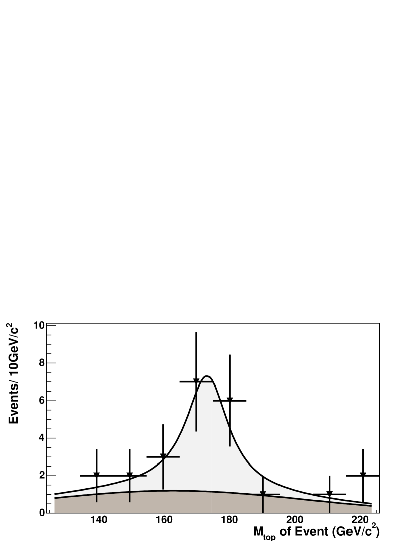
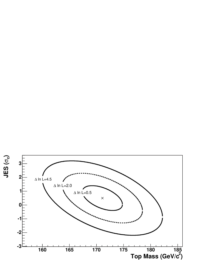
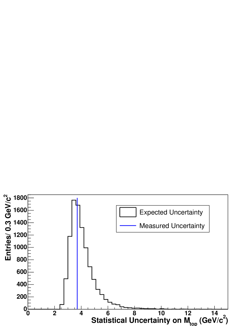
We present a measurement of the top quark mass in the all-hadronic channel ( ) using 943 pb-1 of collisions at TeV collected at the CDF II detector at Fermilab (CDF). We apply the standard model production and decay matrix-element (ME) to candidate events. We calculate per-event probability densities according to the ME calculation and construct template models of signal and background. The scale of the jet energy is calibrated using additional templates formed with the invariant mass of pairs of jets. These templates form an overall likelihood function that depends on the top quark mass and on the jet energy scale (JES). We estimate both by maximizing this function. Given 72 observed events, we measure a top quark mass of 171.1 3.7 (stat.+JES) 2.1 (syst.) GeV/. The combined uncertainty on the top quark mass is 4.3 GeV/.
pacs:
14.65.Ha, 12.15.Ff, 13.85.Ni
††preprint: PRD draft of FAST : v1.0
I Introduction
The top quark plays an important role in particle physics.
Being the heaviest observed elementary particle results in large contributions to electroweak radiative corrections and provides a constraint on the mass of the elusive Higgs boson.
More accurate measurements of the top quark mass are important for precision tests of the standard model.
In addition, having a Yukawa coupling close to unity may indicate a special role for this quark in electroweak symmetry breaking.
Increasing the precision on the mass of the top quark is central not only for the standard model, but also for other theoretical scenarios beyond the standard model.
At the Tevatron the top quark is produced most frequently via the strong interaction yielding a top/anti-top pair.
Once produced, the top quark decays into a quark and a boson about 99% of the time according to the standard model.
Based on the decay mode of the two bosons the events can be divided in three channels: the dilepton channel when both bosons decay to leptons;
the lepton+jets channel when one boson decays to leptons and the other one decays to hadrons;
and the all-hadronic channel when both bosons decay to hadrons.
This paper reports a measurement of the top quark mass in the all-hadronic channel using 943 pb-1 collected with the upgraded CDF II detector at Fermilab.
In Section II we give a brief description of the CDF II detector.
The all-hadronic final state consists of six jets, two of which are due to the hadronization of quarks.
The large QCD background and jet-parton combinatorics make measurements more difficult in this channel than in the others.
However, because there are no unobserved final-state particles, it is possible to fully reconstruct all-hadronic events.
In order to enhance the content over the background, special selection criteria are imposed on the kinematics and topology of the events.
In Section III we give more details on this selection.
Previous mass measurements of the top quark in the all-hadronic channel were performed at CDF in both Run I ahmass1 and Run II ahmass2 .
For the first time in this channel, we measure the mass of the top quark utilizing a technique that uses the matrix element for production and decay.
The details of the matrix element calculation and implementation are given in Section IV.
The matrix element is used to calculate a probability for each candidate event to be produced via the standard model production mechanism.
In principle, the mass of the top quark can be determined by maximizing this probability, and such a technique was successfully applied before at CDF in the lepton+jets channel lepjets and in the dilepton channel dilepton .
In this analysis we take a new approach in that we calculate the matrix element probability in samples of simulated events to build and to parameterize top mass templates.
These are distributions that depend on the mass of the top quark, unlike the templates for background events whose modeling is described in Section V.
The measured value of the mass of the top quark corresponds to a template whose mixture with a background template best fits the data.
In Section VI we give more details on how these templates are built.
Besides considering a matrix element for a different decay channel, in this analysis the matrix element is computed differently than in the aforementioned analyses in the leptonic channels.
Also, the features of the matrix element probability are exploited to improve the event selection.
The uncertainty on the jet energy scale has the largest contribution to the total uncertainty in most top quark mass measurements.
In order to minimize this effect, we perform an in situ calibration of the jet energy scale using the invariant mass of pairs of light flavor jets.
For events this variable is correlated with the mass of the boson, and it is sensitive to variations in jet energy scale.
Using this invariant mass we build the dijet mass templates, and we use them for the calibration of the jet energy scale as shown in Section VI.
This procedure, used previously at CDF for the mass measurement of the top quark in the lepton+jets channel ljjes , is used for the first time in the all-hadronic channel in the analysis described in this paper.
The result of the data fit is the topic of Section VII, while in Section VIII the associated systematic uncertainties are described.
Finally, Section IX concludes the paper.
II Detector
The CDF II detector is an azimuthally and forward-backward symmetric apparatus designed to study collisions at the Tevatron.
It is a general purpose detector which combines precision particle tracking with fast projective calorimetry and fine grained muon detection.
The CDF coordinate system is right handed, with axis tangent to the Tevatron ring and pointing in the direction of the proton beam.
The and coordinates of a left-handed ,, Cartesian reference system are defined pointing outward and upward from the Tevatron ring, respectively.
The azimuthal angle is measured relative to the axis in the transverse plane.
The polar angle is measured from the proton direction and is typically expressed as pseudorapidity ln(tan).
We define transverse energy as sin and transverse momentum as sin where is the energy measured in the calorimeter and is the magnitude of the momentum measured by the tracking system.
Tracking systems are contained in a superconducting solenoid, 1.5 m in radius and 4.8 m in length, which generates a 1.4 T magnetic field parallel to the beam axis.
The calorimeter surrounds the solenoid.
A more complete description of the CDF II detector can be found in Ref. cdf2 .
The main features of the detector systems are summarized below.
The tracking system consists of a silicon microstrip system and an open-cell wire drift chamber that surrounds the silicon.
The silicon microstrip system consists of eight layers in a cylindrical geometry that extends from a radius of r = 1.35 cm from the beam line to r = 29 cm.
The layer closest to the beam pipe is a radiation-hard, single sided detector called Layer 00 l00 .
The remaining seven layers are radiation-hard, double sided detectors.
The first five layers after Layer 00 comprise the SVXII svx2 system and the two outer layers comprise the ISL isl system.
This entire system allows track reconstruction in three dimensions.
The resolution on the impact parameter for high-energy tracks with respect to the interaction point is 40 m, including a 30 m contribution from the beam-line.
The resolution to determine ( position of the track at point of minimum distance to interaction vertex) is 70 m.
The 3.1 m long cylindrical drift chamber (COT) cot covers the radial range from 43 to 132 cm and provides 96 measurement layers, organized into alternating axial and stereo superlayers.
The COT provides full coverage for 1.
The hit position resolution is approximately 140 m and the transverse momentum resolution = 0.0015 GeV/.
Segmented electromagnetic and hadronic sampling calorimeters surround the tracking system and measure the energy flow of interacting particles in the pseudorapidity range 3.6.
The central calorimeters (and the end-wall hadronic calorimeter) cover the pseudorapidity range 1.1(1.3) and are segmented in towers of 15o in azimuth and 0.1 in .
The central electromagnetic calorimeter cem uses lead sheets interspersed with polystyrene scintillator as the active medium and photomultipliers.
The energy resolution for high-energy electrons and photons is 13.5%/2%, where the first term is the stochastic resolution and the second term is a constant term due to the non-uniform response of the calorimeter.
The central hadronic calorimeter cha uses steel absorber interspersed with acrylic scintillator as the active medium.
The energy resolution for single-pions is 75%/3% as determined using the test-beam data.
The plug calorimeters cover the pseudorapidity region 1.1 3.6 and are segmented in towers of 7.5o for 2.1 and 15o for 2.1.
They are sampling scintillator calorimeters coupled with plastic fibers and photomultipliers.
The energy resolution of the plug electromagnetic calorimeter pem for high-energy electrons and photons is 16%/1%.
The energy resolution for single-pions in the plug hadronic calorimeter is 74%/4%.
The collider luminosity is proportional to the average number of inelastic collisions per bunch crossing which is measured using gas Čherenkov counters clc located in the 3.7 4.7 region.
The data selection (trigger) and data acquisition systems are designed to accommodate the high rates and large data volume of Run II.
Based on preliminary information from tracking, calorimetry, and muon systems, the output of the first level of the trigger (level 1) is used to limit the rate of the accepted events to 18 kHz at the luminosity range 37 1031 cm-2s-1.
At the next trigger stage (level 2), with more refined information and additional tracking information from the silicon detector, the rate is reduced further to 500 Hz.
The final level of the trigger (level 3), with access to the complete event information, uses software algorithms and a farm of computers to reduce the output rate to 100 Hz, which is the rate at which events are written to permanent storage.
III Data Sample and Event Selection
The expected signature of a event in the all-hadronic channel ( ) is the presence of six jets in the reconstructed final state.
Jets are identified as clusters of energy in the calorimeter using a fixed-cone algorithm with radius 0.4 in - space jetalg .
The energy of the jets needs to be corrected for various effects back to the energy of the parent parton.
The CDF jet energy corrections are divided into several levels to accommodate different effects that can distort the measured jet energy: non-uniform response of the calorimeter as a function of , different response of the calorimeter to different particles, non-linear response of the calorimeter to the particle energies, uninstrumented regions of the detector, multiple interactions, spectator particles, and energy radiated outside the jet clustering cone.
In this analysis we correct the energy of the jets taking into account all of the above effects except those due to spectator particles and energy radiated outside the cone.
These additional corrections are recovered using the transfer functions defined in Section IV.
A detailed explanation of the procedure to derive the various individual levels of correction is described in Ref. nimjes .
Briefly, the calorimeter tower energies are first calibrated as follows.
The scale of the electromagnetic calorimeter is set using the peak of the dielectron mass resonance resulting from the decays of the boson.
For the hadronic calorimeter we use the single pion test beam data.
This calibration is followed by a dijet balancing procedure used to determine and correct for variations in the calorimeter response to jets as a function of .
This relative correction ranges from about -10 to +15.
After tuning the simulation to reflect the data, a sample of simulated dijet events generated with pythiapythia is used to determine the correction that brings the jet energies to the most probable true in-cone hadronic energy.
The absolute correction varies between 10 and 40.
A systematic uncertainty on these corrections is derived in each case.
Some are in the form of uncertainties on the energy measurement themselves, and some are uncertainties on the detector simulation.
Typical overall uncertainty is in the range of 3 to 4 for jets with transverse momentum larger than 40 GeV/.
More details on the estimation of these uncertainties can be found in nimjes .
The data sample is selected using a dedicated multi-jet trigger defined as follows.
For triggering purposes the calorimeter granularity is simplified to a 24 24 grid in - space.
A trigger tower spans approximately 15o in and 0.2 in covering one or two physical towers.
At level 1, we require at least one trigger tower with transverse energy 10 GeV.
At level 2, we require the sum of the transverse energies of all the trigger towers, , be 175 GeV and the presence of at least four clusters of trigger towers with 15 GeV.
Finally, at level 3 we require four or more reconstructed jets with 10 GeV.
This trigger selects about 80 of the events in the all-hadronic channel.
The main background present in this data sample is due to the production of multi-jets via QCD couplings.
This analysis relies on Monte Carlo event generation and detector simulation to model the events. We use herwig v6.505 herwig for the event generation. The CDF II detector simulation cdfmc reproduces the response of the detector to particles produced in collisions.
Tracking of particles through matter is performed with geant3geant .
Charge deposition in the silicon detectors is calculated using a parametric model tuned to the existing data.
The drift model for the COT uses the garfield package garfield , with the default parameters tuned to match COT data.
The calorimeter simulation uses the gflashgflash parameterization package interfaced with geant3.
The gflash parameters are tuned to test-beam data for electrons and pions.
We describe the modeling of the background in Section V.
The events passing the trigger selection are further required to pass a set of clean-up cuts.
First, we require the reconstructed primary vertex btag in the event to lie inside the luminous region ( 60 cm).
In order to reduce the contamination of the sample with events from the leptonic decays, we veto events which have a well identified high- electron or muon tightlep , and require that be 3 GeV1/2metsig , where the missing transverse energy, met , is corrected for both the momentum of any reconstructed muon and the position of the interaction point. The quantity is the sum of the transverse energies of jets.
After this preselection, we consider events with exactly six jets, each with transverse energy 15 GeV and 2.
With these six jets, we calculate four variables that are used for the kinematic discrimination of from background.
One of these variables is defined above.
Another variable, , is the sum of the transverse energies of jets removing the two leading jets.
We define centrality, , as , where and are the sum of the energies of jets and the sum of the momenta of jets along the -axis, respectively.
The fourth variable is the aplanarity, , defined as .
Here is the smallest normalized eigenvalue of the sphericity tensor , where is the momentum of a jet along one of the Cartesian axes.
We select events which satisfy the following kinematical cuts: + 0.005 0.96, 0.78, and 280 GeV.
More details on the clean-up cuts, kinematical and topological variables as well as the optimization of the cuts are given in Ref. ahxs .
Since the final state of a event is expected to contain two jets originating from quarks, their identification is important for enhancing the content of our final data sample.
Jets are identified as jets using a displaced vertex tagging algorithm.
This algorithm looks inside the jet for good-quality tracks with hits in both the COT and the silicon detector.
When a displaced vertex can be reconstructed from at least two of those tracks, the signed distance () between this vertex and the primary vertex along the jet direction in the plane transverse to the beams is calculated.
The jet is considered tagged if /() 7.5, where () is the uncertainty on .
This algorithm has an efficiency of about 60 for tagging at least one jet in a simulated event.
More information concerning tagging is available in Ref. btag .
In order to improve the signal purity, we require the existence of at least one secondary vertex tag in the event.
We introduce a new variable, , defined as the minimum of the event probability calculated using the matrix element technique (see Section IV for details).
Figure 1 shows the distribution of for a simulated sample with = 175 GeV/ (continuous line) and for the background (dashed line), after kinematical and tagging requirements.
Here and throughout this paper we use to label the top quark mass used in the event generation.
The event probability used in Figure 1 is not normalized due to omission of multiplicative constants in its calculation.
Although technically this variable is not a probability, we will keep using this name.
To further reduce the background contribution, we require that 10.
The value of the cut on is obtained by minimizing the statistical uncertainty on the top quark mass reconstructed using only the matrix element technique.
The optimization was done for various top mass quark values using a combination of simulated events and background events (described in Section V).
Figure 1: Distribution of (minimum of the negative log event probability) for simulated events with = 175 GeV/c2 (continuous) and for background events (dashed) modeled in Section V. The events pass the kinematical and -tagging requirements.
Table 1 shows the observed number of events in the multi-jet data sample corresponding to a integrated luminosity of 943 pb-1 that pass the full event selection.
The table also shows the expected number of events (S) based on a sample of simulated events assuming the theoretical value of 6.7 pb Cacciari for the production cross section.
The signal-to-background ratio (S/B) is also shown, where the number of background events (B) is taken as the difference between the observed number of events and the expectation (S).
Based on the results reported in Table 1, the cut improves the signal-to-background ratio by a factor of three for the sample where only one secondary vertex tag is required, and by a factor of two for the sample where at least two tags are required.
Table 1: Number of observed multi-jet events passing the event selection corresponding to an integrated luminosity of 943 pb-1. The table also shows the expected number of events (S) and the corresponding signal-to-background ratio (S/B). The number of events is based on a sample of simulated events assuming the theoretical value of 6.7 pb Cacciari for the production cross section. The number of background events is taken as the difference between the observed number of multi-jet events and the expectation (S).
Selection
Single Tag
Double Tag
Observed
S
S/B
Observed
S
S/B
Kinematical
782
71
1/10
148
47
1/2
10
48
13
1/3
24
14
1/1
IV Matrix Element Tool
For each event passing our kinematical and topological requirements, we calculate the corresponding elementary cross section assuming production followed by the all-hadronic decay.
In this calculation, we consider the momentum 4-vectors of all the observed six jets, but we assume them to be massless.
The fraction of the total cross section contributed by an event can be interpreted as a probability density for the given event to be part of the production.
As it is shown in Section IV.1, for each event this probability density depends on the top quark mass.
The mass value that maximizes the event probability is used in the top quark mass reconstruction technique described in Section VI.
A likelihood function obtained by combining the probability densities of a set of events can also be used to reconstruct the top quark mass.
We use this technique in subsection IV.2 only to validate the matrix element calculation used in the probability density determination, and not for the final mass reconstruction.
IV.1 Definition of the probability density
For any event defined by a set of six 4-momenta, the elementary cross section at a given top quark mass can be computed as if the event were the result of production followed by all hadronic decay:
(1)
Here, () is the fraction of the proton(antiproton) momentum carried by the colliding partons; and are the parton distribution functions for protons and for antiprotons respectively; and , and and represent the velocities and, respectively, the energies of the colliding partons; is a generic notation for all six 4-momenta in the event assuming perfect parton identification and reconstruction; is the matrix element corresponding to production and decay in the all hadronic channel; () is a generic notation for the 4-vector of the final(initial) state.
If we sum the elementary cross sections of all the events passing our event selection (trigger, kinematical and topological) without the requirement, we obtain a fraction () of the total cross section, :
(2)
The fraction is equivalent to the event selection efficiency for events and is determined using samples of simulated events.
For each event, we define the probability density as
(3)
The quantity is the probability for an event defined by the set of six jets (i.e., six 4-momenta) to be the result of production followed by an all hadronic decay for top quark mass .
The final state partons from decay are observed as jets in our detector.
Using simulated events we calculate transfer functions, , which represent a probability for a parton with momentum to be observed as a jet with momentum .
The transfer functions are described in Section IV.1.3.
In order to enhance the features of the phase space, an additional weight, , is introduced.
As it is shown in Section IV.1.4, this weight is obtained from the distribution of the transverse momentum of the system in simulated events.
We assume that all six jets present in an all-hadronic event are the result of the hadronization of quarks in the final state.
There is an ambiguity in assigning the jets to the quarks, and therefore all the possible combinations are considered and averaged.
The counting of all possible assignments is detailed in Section IV.1.2.
The full expression of the probability density is given by:
(4)
where the sum is performed over all jet-parton combinations and is the total number of possible jet-parton assignments.
The calculation of the matrix element is detailed in Section IV.1.1 and the integration performed in Eq. 4 is described in Section IV.1.5.
IV.1.1 Calculation of the matrix element
Two processes contribute to production: gluon-gluon fusion and quark-antiquark annihilation.
At the Tevatron, about of events are expected to be produced by gluon-gluon fusion while the remaining are produced by quark-antiquark annihilation Cacciari .
In addition, of the simulated events produced by quark-antiquark annihilation result from annihilation.
Given that having both types of production doubles the calculation time, we only use the matrix element describing the process .
To validate this choice, we reconstruct the top quark mass using a matrix element in a sample of events produced only via gluon-gluon fusion.
We observe a negligible bias (0.0 0.2 GeV/) in the reconstruction of the top quark mass and we conclude that using a matrix element with as the initial state should be sufficient for the mass reconstruction.
For the final state, having a boson decay into a pair or a pair results in no difference for the final reconstruction as both pairs of quarks will be observed as jets.
The other hadronic decays are suppressed since their rate is proportional to the square of small elements of the Cabibbo-Kobayashi-Maskawa matrix ckm .
In the high-energy limit (or the massless limit), the solutions to the Dirac equation can be written as
(7)
(10)
where is the 4-momentum of a particle.
The solution with positive frequencies is , and that with negative frequencies is ; and , where are the Pauli spin matrices.
The presence of the operator will project the spin states along the direction of motion defined by . For a particle traveling in the direction defined by the polar angle and by the azimuthal angle , the spin states along this direction are given by Eq. 11.
(11)
For an antiparticle we have and . Given these relations and assuming that the incoming partons travel along the -axis, the matrix element has only two non-zero terms due to the initial state partons, and . These are 4-vectors and correspond to the situations when the incoming partons have the same chirality. Considering the proton going in the positive direction, these terms are:
(12)
where and are the energies of the incident quark and quark, respectively.
Omitting all multiplicative constants, we express the matrix element squared as
(13)
where the factors entering this expression are
(14)
In Eq. 14 and are the mass and the width of the boson, and are the mass and the width of the top quark, and and are the 4-momenta of the bosons.
Also in Eq. 14 stands for both and (Eq. 13), the difference arising from the definition of the symbol .
The symbol is defined as
(15)
where are the Dirac matrices and is either or .
We calculate and using Eq. 11 and matrix algebra peskin .
IV.1.2 Combinatorics
While there are ways to assign the observed jets to the six partons of the final state in all hadronic decay, we can take into account a reduced number of possibilities by making a few observations and assumptions.
In the case of the process , assuming that the masses of the up quarks are negligible and omitting the constant and the gluon propagator terms, the spin averaged matrix element squared is
(16)
where is the 4-momentum of a particle.
From this expression, the symmetry is evident.
The symmetry holds also for the matrix element of the process containing the decay of the top quarks.
This symmetry can be translated into a symmetry to once we consider all possible - pairings for each top quark: . It is obvious that swapping the ’s is equivalent with swapping the top quarks.
In conclusion, due to the symmetry the number of relevant combinations is .
Secondly, if any of the jets is identified as a secondary vertex tag we assume that jet be produced by a quark.
This assumption results in a factor of three reduction of the number of relevant combinations, down to (or ).
If there is an additional secondary vertex tag, we get a factor of five reduction down to (or ).
If there are more than two secondary vertex tags, we assign to quarks only the two jets with the highest transverse energy.
Note that the quarks in the decay of either boson can not be interchanged in the matrix element calculation as one is particle and the other is antiparticle and they have different spinors.
IV.1.3 Transfer functions
The transfer functions, , express the probability for a parton with momentum to be associated with a jet reconstructed to have momentum .
The transfer function term from Eq. 4 is in fact a product of six terms, one for each of the final state quarks: two for the quarks and four for the decay products of the bosons.
For each jet in the final state we assume that the jet axis is the same as that of the parton that went on to form the jet.
Making the change of variables , the expression for becomes:
(17)
where and are the solid angles of the jets and of the quarks, respectively.
The transfer functions are built using simulated events with = 175 GeV/ surviving the trigger, kinematical and topological requirements.
The choice of = 175 GeV/ is arbitrary as our studies show that the transfer functions have a negligible dependence on the mass of the top quark in the range 150 GeV/ to 200 GeV/.
In this sample, we associate a jet with a parton if their separation in the space is .
We define a jet to be matched to a parton if no other jet satisfies this geometrical requirement.
We define a event to be matched if each of the six partons in the final state has a unique jet matched to it.
The transfer functions are built out of the sample of matched events.
The jets formed by partons from -bosons decays have a different energy spectrum from that of the jets originating from the quarks.
Thus we form different sets of transfer functions depending on the flavor of the parton the jet has been matched to.
The transfer functions are described using a parameterization in bins of the parton energies and of the parton pseudorapidities.
We use three bins for the pseudorapidity: , , and .
Table 2 shows the definition of energy binning for the -jet transfer functions, while Table 3 is for the -jet transfer functions.
The energy binning is chosen such that the distributions for transfer functions are smooth.
In each bin, the shape of the transfer function is fitted to a normalized sum of two Gaussians.
Table 2: Definition of the binning of the parton energy for the -jet transfer functions parameterization for various bins. The unit for the energy values is GeV.
Bin
1
2
3
4
5
6
7
Table 3: Definition of the binning of the parton energy for the -jet transfer functions parameterization for various bins. The unit for the energy values is GeV.
Bin
1
2
3
4
5
6
7
8
9
10
11
12
13
14
IV.1.4 Transverse momentum of the system
The weight (introduced in Eq. 4) is a function dependent on the momenta of the partons in the final state, generically represented by in the argument of the function.
More exactly, this weight depends on the magnitude of the transverse momentum of the system, , and azimuthal angle, .
As we expect to have a flat dependence on we express this through a factor of .
We define the function to express the dependence on .
We write in Eq. 18 the expression of the weight due to the transverse momentum of the system.
(18)
where is shown in its Cartesian form using the projections of the transverse momentum of the system along the and axes.
Using the same simulated events as for transfer functions, in Fig. 2 we show the distribution of the magnitude of the transverse momentum of the system. A sum of three Gaussians is a good fit of this distribution.
Figure 2: Magnitude of the transverse momentum of the system in simulated events. The fit is a sum of three Gaussians.
IV.1.5 Implementation and evaluation of the probability density
The Sections IV.1.2, IV.1.1, IV.1.3 and IV.1.4 present details on the expressions of several important pieces entering the probability density.
To carry out the integration over parton momenta, we change to a spherical coordinate system.
The delta functions present in the expression of the transfer functions (Eq. IV.1.3) allow us to drop all integrals over the parton angles.
To further reduce the number of integrals we use the narrow width approximation for the bosons.
This results in two more delta functions for the squares of the propagators of the two bosons exemplified in Eq. IV.1.5 for both bosons.
(19)
In the high-energy limit, the invariant mass of the -boson decay products is given by:
(20)
where is the difference in pseudorapidities of the two decay partons and is the difference between their azimuthal angles.
Making the change of variables , Eq. IV.1.5 can be written as:
(21)
where .
In the case of the boson we use equations similar to Eqs. IV.1.5 and 21, but with different notations: the change of variables is and the pole of the delta function is .
The mass and width of the boson are fixed at 80.4 GeV/ and 2.1 GeV/, respectively pdg .
As described in section IV.1.1, we assume that the incoming partons have zero transverse momentum.
This would, in principle, result in violation of momentum conservation in the transverse plane as we consider non-zero transverse momentum for the system in the ME calculation. However, we expect this to be a small effect covered by the uncertainty on the parton distribution functions of the proton and of the antiproton. We can omit the delta functions requiring energy conservation along the and axes, resulting in
(22)
We make the change of variables and since and .
The values of the proton and antiproton momenta, and , are constant and from now on we drop them from any expressions.
In the high-energy limit we have and we omit this term since is a constant, the speed of light.
We express the energy-conserving delta function as
(23)
where and .
In section IV.1.4, we expressed as a function of the projections of the transverse momentum of the system along the and axes (Eq. 18). We will make a change of variable from the -quark momenta to these variables. The Jacobian of this transformation
(24)
is obtained by solving the system of equations for and .
(25)
We write the expression of the probability density in its final form as
(26)
We evaluate the integrals in Eq. IV.1.5 numerically.
The integration is performed in the interval GeV/ for the variables and GeV/ for the variables .
The step of integration is 2 GeV/.
Based on a sample of events where = 175 GeV/ passing the event selection, we choose these integration ranges such that the distributions of the parton level variables ( and momenta of -boson decay partons) are contained well (99) within them.
Given these limits, at each step of integration we have to make sure that all momenta entering Eq. IV.1.5 have positive magnitudes.
The probability density is evaluated for top mass values going in 1 GeV/ increments from 125 GeV/ to 225 GeV/.
The dependence on mass of the cross section is obtained from values calculated at leading-order by comphepcomphep Monte Carlo generator for the processes , and .
The absolute values for these cross sections are not as important as their top mass dependence, which is shown in Fig. 3.
Figure 3: Cross section for production as a function of the top quark mass, as obtained from comphepcomphep .
For the proton and antiproton parton distribution functions (PDF), , we use the cteq5lcteq5l distributions with the scale corresponding to a top mass of 175 GeV/. The acceptance, , is described in Section IV.1.
IV.2 Validation of the matrix element calculation
The event probability described in the Section IV.1 is expected to have a maximum around the true top quark mass in the event.
Multiplying all the event probabilities we obtain a likelihood function,
(27)
which is expected to have a maximum around the true top quark mass of the sample.
Finding the value of the top quark mass that maximizes the likelihood represents the traditional method for reconstructing the top quark mass using a matrix element technique dilepton .
However, we use this reconstruction technique only to check the matrix element calculation.
We use the simulated samples generated with various top quark masses.
For each sample, we reconstruct the top quark mass using the traditional matrix element technique and compare the reconstructed mass to the true input mass for several different input mass values.
Ideally, we should see a linear dependence with no bias and a unit slope.
The first check is done at the parton level.
We smear the energies of the final state partons from our simulated events and use these numbers to describe the jets.
The parton energies are smeared according to the transfer functions described in section IV.1.3.
Figure 4 shows the linearity check in this case.
We observe a slope of 1 and a bias of 0.9 GeV/.
We perform the same test using the energies of the jets matched to the partons.
Figure 5 shows the linearity check.
Here the bias is 1.2 GeV/, but the slope remains 1.
The final test we perform to validate the matrix element calculation uses fully reconstructed signal events where we allow events to include mismatched jets as well.
Figure 6 shows the linearity check in this case.
The bias is no longer the same for all masses as the slope is 0.94 0.01.
Figure 4: Reconstructed top mass versus input top mass at parton level. The energies of the partons have been smeared using the transfer functions. The continuous line is added for visual reference.Figure 5: Reconstructed top mass versus input top mass using jets that were uniquely matched to partons. The continuous line is added for visual reference.Figure 6: Reconstructed top mass versus input top mass using realistic jets. The continuous line is added for visual reference.
Although there is some bias, all checks we list above show the good performance of our matrix element calculation.
In general, the traditional matrix element approach lepjets is expected to provide a better statistical uncertainty on the top mass than the template analyses ljjes .
In the case of the present analysis, our studies show that the traditional matrix element method does better only when the mass reconstruction is performed on signal samples.
When the background is mixed in, the template method we use has a greater sensitivity and by construction eliminates the bias of the matrix element calculation (see Section VI).
V Background Model
In this section we describe the data-driven technique used to model the background for this analysis.
The technique uses jet energies which are measured in the calorimeter and so are unchanged by jet energy scale changes.
Properties of the model are checked by comparison with a simulated sample of events containing the final state + 4 light partons.
The modeling of background is based on a subset of the multi-jet data sample depleted of events where the heavy flavor jets are identified according to background-like heavy flavor rates (tagging matrix), described in Section V.1.
The subset of multi-jet data is selected applying the event selection of Section III excluding the and the secondary vertex tag requirements.
This sample (BG) counts 2652 events, with an estimated signal-to-background ratio of about 1/25.
For this ratio we estimate the signal from a sample of simulated events assuming a production cross section of 6.7 pb.
The estimate for the background is equal to the number of observed events in the BG sample.
V.1 Tagging matrix
The tagging matrix is a parameterization of the heavy flavor rates as a function of the transverse energy of jets, the number of tracks associated to the jet and the number of primary vertices in the event.
Using the -tagging algorithm described in Section III, we determine the above rates in a sample (4J) largely dominated by QCD multi-jet processes and selected from multi-jet data events with exactly four jets and passing the clean-up requirements described in Section III.
We use a control region to check our assumption that the tagging rates from the 4-jet sample can be used to predict the tagging rates as a function of the variables used in the kinematical selection.
This control region (CR1) contains events with exactly six jets and passing the clean-up cuts.
The signal-to-background ratio in this region is about 1/250, estimated using same method as for the BG sample.
We compare the observed rates with the predicted rates based on the tagging matrix.
Figure 7 shows the comparison for events with exactly one secondary vertex tag, while Fig. 8 shows the comparison in the sample with at least two secondary vertex tags.
The variables chosen for this comparison are the transverse energies of jets, sum of the transverse energies of the six leading jets, aplanarity, and centrality as defined in Section III.
The Kolmogorov-Smirnov probabilities for these comparisons in the single (double) tagged samples are: 0.0 (8.6E-5), 3E-11 (0.69), 0.99 (4.3E-3), and 0.12 (0.05), respectively.
Based on Fig. 7(a), the discrepancy between the observed rate and the predicted rate for jets with low transverse momentum may be an artifact of the binning of the tagging matrix.
For transverse energies between 15 GeV and 40 GeV the tagging matrix uses the average rate, and therefore the rates for smaller intervals in this range might not be predicted well.
Figures 7(a) and 8(a) support this by showing that, for this range of transverse energies, half of the data points are below and the other half is above the solid histogram representing our background model.
The overall agreement between the observed and predicted rates is quite poor. In principle, a systematic uncertainty should be assigned to cover this discrepancies. However, the templates used in the mass measurement use the event probability based on matrix element information and they will be less affected by these inaccuracies. The reason for this is the fact that we use only a matrix element. For background events the event probability (Eq. IV.1.5)is flat as a function of the assumed top quark mass. The flatness of the event probability results in wide templates for the background sample and the systematic effects due to the mistag matrix will get smeared. In fact, the background templates in the control regions defined in Section V.2 agree very well with the corresponding distributions based on the simulation of background events with + 4 light partons in the final state.
We conclude that the tagging matrix can be used to predict the background-like heavy flavor rates for events with same jet multiplicity as expected for the all-hadronic events.
More details on the tagging matrix can be found in Ref. ahxs .
Figure 7: Background validation in control region CR1 for single tagged events from the multi-jet data (dots) and from the background model (solid histogram). The distributions are normalized to the same area.Figure 8: Background validation in control region CR1 for double tagged events from the multi-jet data (dots) and from the background model (solid histogram). The distributions are normalized to the same area.
V.2 Estimation of the background
Based on the tagging matrix, a jet has a certain probability (rate) to be tagged as a heavy flavor jet depending on its transverse energy, number of tracks associated to it and number of vertices in the event.
For a jet with a transverse energy between 15 GeV and 40 GeV and with ten associated tracks, this probability is (7.2 0.5).
Using these probabilities we tag the jets as originating from a quark.
This tagging procedure is repeated 20,000 times in the events of the BG sample producing about ten million tagged configurations which are interpreted as background events.
A tagged configuration is an event from the BG sample where at least one of the six jets is tagged using the tagging matrix.
Such kind of event can produce many tagged configurations which are unique if they have different tagged jets or a different number of tagged jets.
We find 12888 unique single tagged configurations, and 26715 unique double tagged configurations.
Of these, 657 (or (5.1 0.2)) single tagged configurations and 1180 (or (4.4 0.1)) double tagged configurations pass the cut.
We use these configurations, unique or duplicate, to form all relevant background distributions used for various checks and for the final measurement.
The estimated number of background events is defined as the difference between the total number of events observed in the data sample and the expected number of events based on the standard model expectation for production cross section of 6.7 pb Cacciari .
This normalization applies to the top quark mass reconstruction procedure described in Section VI, and for the validation of the background model described below.
We check various distributions of the background events modeled above against those from a sample of simulated events with + 4 light partons in the final state.
This simulated sample is built using alpgenalpgen for the event generation, pythia for the parton showering, and the detector simulation as described in Section III.
Given our event selection, other background sources are expected to have smaller contributions compared to the one from + 4 light partons and therefore affect less the relevant distributions.
This check is performed in a control region (CR2) and in the signal region (SR) defined as follows.
Region CR2 contains events that pass all our selection requirements without the cut and has a signal-to-background ratio of about 1/6.
The signal region SR has events passing all selection criteria defined in Section III.
Table 4 summarizes all the regions used in our background modeling procedure.
Table 4: Definition of the control regions used in the background modeling procedure. The selection requirements that differentiate them are defined in Section III.
Region
Clean-up
Kinem.
-tag
4J
yes
4
no
no
no
2,242,512
BG
yes
6
yes
no
no
2652
CR1
yes
6
no
no
no
380,676
CR2
yes
6
yes
no
yes
930
SR
yes
6
yes
yes
yes
72
Given that the BG sample used in our background model contains a small content, we need to correct all the background distributions built from it.
The relationship between a given uncorrected background distribution, , and the corrected one, is
(28)
where is the corresponding distribution for events and is the fraction of the uncorrected background sample due to events.
These quantities for are determined from a sample of simulated events where = 170 GeV/ by randomly tagging the jets using the tagging matrix defined in Section V.1.
We choose the above value for the top quark mass based on the value of the world mass average massavg at the time of this analysis; in Section VIII we determine a systematic uncertainty due to this choice.
The expression for in region CR2 is
(29)
where is the background estimate in this region and is the number of events estimated using the tagging matrix.
The expression for in region SR is
(30)
where () is the efficiency of the cut for (background) in the CR2 region.
The efficiency for background is determined using the ratio of the number of uniquely tagged configurations before the cut (12,888 single tagged and 26,715 double tagged), and after the cut respectively (657 single tagged and 1180 double tagged).
Table 5 shows the estimated number of background events and the efficiency of the cut for background in region CR2.
Tables 6 and 7 show the values for , , and in region CR2 as well as the values of for simulated samples with different values on .
Table 5: The estimated number of background events and the efficiency of the cut for background in region CR2. The number of background events is the difference between the observed number of events and the expected number of events assuming a production cross section of 6.7 pb.
Parameter
Single Tag
Double Tag
711
101
0.051
0.044
Table 6: The number of events, , with one jet identified as jets using the tagging matrix; in region CR2, the acceptance of the cut for events, , and the values of the parameters (Eq. 29), and (Eq. 30) for simulated samples with different values on .
(GeV/)
160
29
0.21
0.039
0.146
170
30
0.20
0.040
0.144
175
28
0.19
0.038
0.130
180
28
0.18
0.038
0.124
Table 7: The number of events, , with at least two jets identified as jets using the tagging matrix; in region CR2, the acceptance of the cut for events, , and the values of the parameters (Eq. 29), and (Eq. 30) for simulated samples with different values on .
(GeV/)
160
2
0.31
0.019
0.133
170
2
0.29
0.019
0.126
175
2
0.29
0.019
0.126
180
2
0.27
0.019
0.118
The correction procedure uses by default the parameters as derived for = 170 GeV/.
In the determination of the systematic uncertainty due to this choice, we use the parameters corresponding to = 160 GeV/, and = 180 GeV/, respectively (see Section VIII).
The parameters obtained using = 175 GeV/ are given for reference in Table 6 as that mass value corresponds to a production cross section of 6.7 pb.
Following this correction procedure, we compare shapes between our background model and the sample of simulated + 4 light partons described above.
First, we do this comparison in region CR2 where we look at the invariant mass of all the untagged pairs of jets in the event (Fig. 9).
The values of the Kolmogorov-Smirnov probabilities are 25 for the samples with single tagged events, and 43 for the samples with double tagged events.
For the signal region, we look at the invariant mass of all the untagged pairs of jets in the event (Fig. 10) and at the most probable per-event top quark mass (Fig. 11).
These are variables of particular interest in this region as they will be used in the reconstruction of the top quark mass and for the in situ calibration of the jet energy scale, as described in Section VI.
Based on the comparison from Fig. 10, the Kolmogorov-Smirnov probabilities are 90 for the single tagged events and 70 for the double tagged events.
(a)(b)
Figure 9: Invariant mass of pairs of untagged jets in control region CR2 for alpgen + 4 light partons (cross), and for the background model (solid): (a) for single tagged events (Kolmogorov-Smirnov probability is ) and (b) for double tagged events (Kolmogorov-Smirnov probability is ).
(a)(b)
Figure 10: Invariant mass of pairs of untagged jets in signal region for alpgen + 4 light partons (cross), and for the background model (solid): (a) for single tagged events (Kolmogorov-Smirnov probability is ), and (b) for double tagged events (Kolmogorov-Smirnov probability is ).
(a)(b)
Figure 11: Event by event most probable top quark masses in the signal region for alpgen + 4 light partons (cross), and for the background model (solid): (a) for single tagged events, and (b) for double tagged events.
These comparisons show good agreement between our data-driven background model and a simulated sample of events containing the final state + 4 light partons, obtained using the alpgen generator.
In Section VIII we evaluate the effect on the reconstructed top quark mass due to the limited statistics available in sample BG to construct the background model.
VI Top Quark Mass Estimation
Our technique starts by modeling the data using a mixture of signal events obtained from simulation and of background events obtained via our background model.
The events are represented by two variables: the invariant mass of pairs of untagged jets and an event-by-event reconstructed top mass described below.
These two variables are used to form distributions (templates), separately for events and for background events.
In the case of events, the templates are parameterized as a function of the mass of the top quark and the jet energy scale (JES) variable (defined below).
For background no such dependences are expected since they contain no top quark and the jet energies used for the background modeling are taken from data.
The measured values for the top quark mass and for the JES are determined using a likelihood technique described in Section VI.2.
The largest contribution to the systematic uncertainty on the top quark mass is due to the uncertainty on the jet energy scale.
To limit the impact of this systematic on the total uncertainty on the top quark mass, we use an in situ calibration of the jet energy scale via the -boson mass.
We measure a parameter JES that represents a shift in the jet energy scale from our default calibration as defined in Section III.
This quantity is expressed in units of the total nominal jet energy scale uncertainty that is derived following the default calibration.
This uncertainty depends on the transverse energy, pseudorapidity, and the electromagnetic fraction of the jet energy.
On average, the uncertainty is approximately equivalent to a 3 change in the jet energy scale for jets in events.
By definition, JES = 0 represents our default jet energy scale; JES = 1 corresponds to a shift in all jet energies by one standard deviation; and so on.
The templates for events are determined from samples of simulated events with ranging from 150 GeV/ to 200 GeV/ in steps of 5 GeV/.
We also include the sample where = 178 GeV/ for a total of twelve different simulated mass samples.
In addition to the variation of the top quark mass, for each value of we consider seven values for JES between -3 and 3 , in steps of 1 .
We use the events obtained from our background model to form the templates for the background.
VI.1 Definition and parameterization of the templates
The first set of templates, called the top templates, is built using a variable () determined using the matrix element technique.
We call the event-by-event reconstructed top quark mass, and it represents the mass value that maximizes the event probability defined in Section IV.
We find the value of by evaluating the event probability in the range 125 GeV/ 225 GeV/.
When building the templates, we drop the events for which the event probability is naturally maximized at mass values outside this range.
These events accumulate at the edges of the distribution making difficult the parameterization described below.
For events, the function used to describe the shape of these templates is a normalized product of a Breit-Wigner function and an exponential:
(31)
where the parameters depend on and on JES.
The normalization is set by that has the following expression:
(32)
The parameters (Eq. 31) depend on and JES as follows:
(33)
In Eqs. VI.1 and 33 the parameters are constants determined from the simultaneous fit of the top templates from all 84 samples with the function .
Figure 12 shows the function for JES = 0 and various values of in the case of events with one tagged jet.
A similar parameterization is obtained for events with at least two tagged jets.
Figure 12: The function fitting the top templates for events at nominal JES and for various hypotheses of the top quark mass in the case of events with one tagged jet. A similar parameterization is obtained for events with at least two tagged jets.
To determine how well the parameterization in Eq. 31 describes the templates, we calculate the divided by the number of degrees of freedom, , as follows
(34)
where is the bin content of the template histogram and is the value of the function from Eq. 31 at the center of the bin.
In Eq. 34, the first two sums in the numerator are over the templates built from simulated events for a given (12 values) and JES (7 values).
The third sum is over all the bins with more than 5 entries from each template.
We obtain for the sample with one secondary vertex tag and for the sample with two secondary vertex tags corresponding to very small probabilities.
From the values of the quantity , we conclude that the parameterization of the top templates is not very accurate, and we expect some bias in the reconstruction of mass and JES.
The procedure for bias removal is described in Section VI.3.
The top templates for background events are built using the matrix element in the same way as for events.
The shape of the background template is fitted to a normalized Gaussian.
Figure 13 shows separately the resulting parameterized curves of background templates for single and double tagged background events.
(a)(b)
Figure 13: Top templates for (a) single tagged background events and for (b) double tagged background events.
The second set of templates, the dijet mass templates, are formed by considering the invariant mass of all possible pairs of untagged jets in the sample.
This variable is correlated to the mass of the boson, and plays a central role in the in situ calibration of the jet energy scale.
For events the function used to fit the dijet mass templates is a normalized sum of two Gaussians and a Gamma function:
(35)
where the parameters depend on and on JES.
The normalization is set by that has the following expression:
(36)
The parameters depend on and JES as follows:
(37)
In Eqs. VI.1 and 37 the parameters are constants determined from the simultaneous fit of the top templates from all 84 samples with the function .
Figure 14 shows the function for = 170 GeV and various values of JES in the case of events with one tagged jet.
A similar parameterization is obtained for events with at least two tagged jets.
Figure 14: The function fitting the dijet mass templates for events with = 170 GeV/ and various values of JES in the case of events with one tagged jet. A similar parameterization is obtained for events with at least two tagged jets.
As in the case of top templates, we calculate (Eq. 34) the quantity to describe the performance of the parameterization of the dijet mass templates.
We obtain for the sample with one secondary vertex tag and for the sample with at least two secondary vertex tags.
From the values of the quantity we reach the same conclusion as in the case of the parameterization of top templates: the parameterization of the dijet mass templates is not very accurate and some bias is expected when the top mass and JES are reconstructed.
The dijet mass template for background is built in the same way as for the templates.
The background template is fitted to a normalized sum of two Gaussians and a Gamma function.
This combination of functions provided the best fit of the dijet mass shapes.
Figure 15 shows separately the resulting parameterized curves of background templates for single and double tagged background events.
(a)(b)
Figure 15: Dijet mass templates for (a) single tagged background events and for (b) double tagged background events.
VI.2 Likelihood definition
The mass of the top quark and the value of JES are determined by maximizing a likelihood function built using the two sets of templates described in Section VI.1.
Assuming that the data sample is the sum of events and background events, we can calculate the likelihood function connected to a generic template as
(38)
where index can either be when the variable represents the event-by-event reconstructed top mass, or for the invariant mass of pairs of light flavor jets.
The number of events, , is constrained to the expected number of events, , via a Gaussian
(39)
with mean equal to and width equal to , the uncertainty on the expected number of events.
The expected numbers of signal events, , are 13 for the single tagged sample and 14 for the double tagged sample corresponding to a theoretical cross section of pb Cacciari and an integrated luminosity of 943 pb-1.
The value of the theoretical cross section assumes a top quark mass of 175 GeV/.
The values for are 3.7 for the single tagged sample and 3.9 for the double tagged sample, which take into account both statistical effects (assuming a Poisson distribution) on and systematic ones based on the uncertainty on the theoretical cross section.
The sum of and background events, , is constrained to the total number of observed events in the data, , via a Poisson probability with a mean equal to
(40)
Multiplying the terms expressing the constraints on the number of events and the likelihood functions for each template, we obtain separate likelihood functions for events with one tag and for events with at least two tags:
(41)
As described in Section III, the jet energy scale JES can be determined from independent detector calibrations.
We include this knowledge in the likelihood in the form of a Gaussian constraint on our variable JES.
This Gaussian has a mean equal to the expectation on JES from the independent calibration, JESexp = 0 , and a width equal to 1 which is the uncertainty on this expectation.
(42)
The term expressing the constraint on the JES variable is multiplied together with the likelihood function for each heavy flavor sample to obtain the final likelihood function used to reconstruct the top quark mass shown in Eq. 43.
(43)
Following the maximization of the likelihood function shown in Eq. 43 we will obtain six numbers: the reconstructed top quark mass , the reconstructed JES variable , and the number of events with different number of tags for , , and for background, .
The statistical uncertainties on these numbers, , , , and are obtained from the points where the log-likelihood changes by 0.5.
VI.3 Calibration of the method
Using samples of simulated events and the background sample built based on the model presented in Section V, we form simulated experiments for a series of JES and input values.
We then verify that the reconstructed values of the top quark mass and JES obtained following the maximization of the likelihood function (Section VI.2) are in agreement with the input values.
The simulated experiments are a mixture of events and background events reflecting the expected sample composition of the data.
In each simulated experiment, the number of events is drawn from a Poisson distribution of mean equal to the expected number of events passing the selection, as determined from simulation (Table 8).
The number of background events is also drawn from a Poisson distribution with a mean equal to the difference between the observed number of events (see Section III, Table 1) and the expected number of events.
Table 8: Number of events for samples of simulated events with ranging between 150 GeV/ and 200 GeV/. The numbers correspond to a integrated luminosity of 943 pb-1, after all selection requirements are made. The observed number of events is also shown.
(GeV/)
Single Tag
Double Tag
150
18
14
155
17
15
160
16
14
165
16
14
170
15
14
175
13
14
178
14
14
180
12
13
185
11
11
190
9
11
195
9
10
200
7
8
Total Observed
48
24
In order to reduce the statistical uncertainties on potential biases in mass or JES reconstruction, about 10,000 simulated experiments are performed.
Due to the finite size of simulated event samples and background sample the simulated experiments share events between them.
These overlaps result in correlations between the results of the mass and JES reconstructions from each simulated experiment.
These correlations are taken into account following the study found in Ref. Barlow .
The typical value for the correlation between any two simulated experiments is 6.
The variables extracted from each simulated experiment are: the values of mass, , and JES, that maximize the likelihood defined in section VI.2; the statistical uncertainties on the above variables, and and the pulls for these variables as defined by
(44)
where JEStrue is the value of JES used in the simulation.
The distribution of the top quark masses reconstructed in each simulated experiment is fitted to a Gaussian.
The mean of this Gaussian is interpreted as the reconstructed top quark mass of the sample, , while the width of the Gaussian represents the expected statistical uncertainty on it, .
We apply the same procedure to determine the reconstructed value of JES, , and its expected statistical uncertainty, .
Figure 16: JES versus Top Quark Mass plane. The points represent the reconstructed JES, , and top quark mass and have attached their corresponding statistical uncertainties, and . The vertical dashed lines correspond to the true values of the mass, while the horizontal lines correspond to the true values of JES. For a perfect reconstruction the points should sit right at the intersection of the dashed lines.
Figure 16 shows the reconstructed JES and the reconstructed top mass represented by the points, versus the true JES and true top mass represented by the grid.
Ideally the points should match the grid crossings, but there is a slight bias which has to be removed.
The bias is removed in the mass-JES plane by solving the system in Eq. 45
(45)
for and JEStrue.
The parameters , , , and have the form
(46)
where the parameters and from Eq. 46 are listed in Table 9.
They are determined from a linear fit of the distributions of and versus JEStrue (Figs. 17 and 18), and of and versus , respectively (Figs. 19 and 20).
Figure 17: Distribution of parameter (Eq. 46) as a function of JES.Figure 18: Distribution of parameter (Eq. 46) as a function of JES.Figure 19: Distribution of parameter (Eq. 46) as a function of .Figure 20: Distribution of parameter (Eq. 46) as a function of .
Table 9: Values of the parameters describing best the linear dependence on the true JES and on the true , of the intercept and slope of the calibration curve and of the JES calibration curve respectively.
Parameter
Value
Uncertainty
175.
0
0.
1
-0.
09
0.
05
0.
975
0.
008
0.
016
0.
004
0.
6
0.
3
-0.
003
0.
002
1.
35
0.
15
-0.
0021
0.
0008
The uncertainties and on the reconstructed values and JESout are also affected by the bias in the reconstruction technique and we need to correct them as well.
By differentiating Eq. 45 with respect to and JEStrue, we obtain another system of equations to be solved for the corrected uncertainties, and .
(47)
The parameters , , , and from Eq. 47 depend on and JEStrue as shown in Eq. 48.
Solving Eq. 47 provides the best estimate of the uncertainties on and on JESout.
(48)
Following the procedure for removing the bias in the mass reconstruction, the distribution of pull means extracted using simulated experiments (Fig. 21) validates our bias correction as, on average, the pull mean is estimated to be consistent with zero within the uncertainty.
The width of the pull distribution is used to determine the corrections on the statistical uncertainties due to non-Gaussian behavior of the likelihood function (Eq. 43).
Figure 22 shows the mass pull widths versus top quark mass .
In these plots the JEStrue of the samples is 0 .
Similar pulls are obtained from samples with different values of JEStrue.
Based on these figures, it is estimated that the uncertainty on has to be increased by 11.
Figure 21: Pull means versus in the case of the reconstruction of top quark mass in samples with JEStrue = 0 . The continuous line represents the average pull mean and the dashed lines show the uncertainty on it.Figure 22: Pull widths versus in the case of the reconstruction of top quark mass in samples with JEStrue = 0 . The continuous line represents the average pull width and the dashed lines show the uncertainty on it.
For the reconstruction of JES, Fig. 23 shows the pull means versus JEStrue, while Fig. 24 shows the pull widths versus JEStrue.
In both plots, = 170 GeV/.
Similar pulls are obtained from samples with different values of .
Regarding the bias correction, we reach the same conclusion as in the case of the mass reconstruction that, on average, the pull mean is estimated to be consistent with zero within the uncertainties.
Based on Fig. 24, it is estimated that the uncertainty on the JESout has to be increased by 6.
Figure 23: Pull means versus in the case of the reconstruction of JES in samples with = 170 GeV/. The continuous line represents the average pull mean and the dashed lines show the uncertainty on it.Figure 24: Pull widths versus versus in the case of the reconstruction of JES in samples with = 170 GeV/. The continuous line represents the average pull width and the dashed lines show the uncertainty on it.
In order to further establish the robustness of the technique, the mass and JES are measured in samples for which the true values are unknown to the authors of this paper.
To validate the mass reconstruction we utilize five such blind samples: three generated with Herwig and two with Pythia.
The value of JES in these samples corresponds to 0, the nominal jet energy scale.
The reconstructed top quark mass in each of these samples is the most probable value obtained from 10,000 simulated experiments.
Each simulated experiment is formed combining the events in the blind samples and the background events from the background model such that on average the total number of events is equal to the observed value (see Table 8).
The size of the content is 15 single tagged events and 14 double tagged events.
Following the mass reconstruction technique and the calibration described in this paper, the differences between the true top quark mass values and the reconstructed ones are: -0.2, 0.3, 0.6, -0.7, and 1.1 GeV/.
The statistical uncertainty on these numbers is 0.8 GeV/.
The first two numbers correspond to the Pythia samples.
To validate the JES reconstruction, another five blind samples are used for which the jet energy scale is modified.
The generator used here is Herwig and the value of the top quark mass is 170 GeV/.
The differences between the true JES values and the reconstructed ones are: 0.1, 0.3, 0.0, 0.1, and -0.1 .
The statistical uncertainty on these numbers is 0.4 .
In conclusion, both the mass and JES reconstructed values are compatible with true ones within the statistical uncertainties.
This additional check gave us confidence that the method described here can be reliably applied on the data to reconstruct JES and the top quark mass.
VI.4 Expected statistical uncertainty
Figure 25: Expected uncertainty on top quark mass, , versus , for samples with JEStrue = 0 . This uncertainty includes the uncertainty due to statistical effects and the systematic uncertainty due to jet energy scale.Figure 26: Expected uncertainty on JES, , versus JEStrue, for samples with = 170 GeV/.
In Fig. 25 we show the expected uncertainty on top quark mass, , versus , for samples with JEStrue = 0 .
Since the expected number of events depends on the , the uncertainty depends on it too.
Figure 26 shows the expected uncertainty on JES, , versus JEStrue, for samples with = 170 GeV/.
The uncertainties in Fig. 25 and 26 are corrected for bias, but not for pull widths (non-Gaussian effects).
The expected uncertainties shown in Fig. 25 contain both the statistical uncertainty on the top quark mass and the uncertainty due to jet energy scale.
In order to disentangle the statistical uncertainty on from the one due to jet energy scale, we reconstruct the top quark mass by maximizing the likelihood for a fixed value of JES.
Following this reconstruction for = 170 GeV/ and JEStrue = 0 , the uncertainty on the top quark mass is 2.5 GeV/.
In comparison, when JES is not fixed the expected uncertainty (Fig. 25) on is 3.2 GeV/.
Subtracting these two numbers in quadrature we estimate that the systematic uncertainty on due to jet energy scale is 2.0 GeV/.
We can determine the systematic uncertainty on due to the jet energy scale in the absence of the in situ calibration (provided by the dijet mass templates), by removing the parameterization as a function of JES and by maximizing a likelihood built only with the top templates corresponding to JES = 0 .
We reconstruct the top quark mass for two samples with = 170 GeV/, but with different values for JEStrue: +1 , and -1 , respectively.
Taking half of the difference between the two reconstructed determines the systematic uncertainty due to jet energy scale as 2.2 GeV/, which is more than in the case of using the in situ calibration and the JES parameterization.
VII Results
Applying the event selection described in Section III to the multijet data corresponding to an integrated luminosity of 943 pb-1, we observe 48 events with one secondary vertex tag and 24 events with at least two secondary vertex tags.
Performing the likelihood maximization and applying the corrections described in Section VI for this sample, we measure a top quark mass of 171.1 3.7 GeV/ and a value for JES of 0.5 0.9 .
Figure 27 shows the distributions of reconstructed top quark masses for data (dots) and for the combination (light) of signal and background templates that best fit the data.
The background (dark) contribution is shown normalized to the data as determined by the fractions obtained from the likelihood fit.
There are two sets of distributions corresponding to the sample with only one secondary vertex tag (Fig. 27(a)) and to the sample with at least two secondary vertex tags (Fig. 27(b)).
(a)(b)
Figure 27: Reconstructed top mass for data (points), best signal+background fit (light) and background shape from the best fit (dark): for (a) samplee with only one secondary vertex tag, and (b) the sample with at least two secondary vertex tags.
The minimized negative log-likelihood is shown in Fig. 28 as a function of the top mass and JES after correcting for bias (Eqs. 45 and 47) and for non-Gaussian effects (Section VI.3).
The central point corresponds to the minimum of the negative log-likelihood, while the contours are given at a number of values of ln, the change in negative log-likelihood from its minimum.
Figure 28: Contours of the likelihood in the Mtop and JES plane at a number of values of , the change in negative log-likelihood from its maximum.
Table 10 lists the number of events for and for background for the one- and two-secondary vertex tags cases, as measured following the minimization of the two dimensional likelihood of Eqn. 43 on the data.
Table 10: Measured sample composition of the multijet data sample for a luminosity of 943 pb-1, passing the event selection. The second column (1 tag) gives the number of events with only one secondary vertex tag, while the third column (2 tags) is for the events with at least two secondary vertex tags.
Number of Events
1 tag
2 tags
Signal ( )
13.2 3.7
14.1 3.4
Background
34.6 7.2
9.2 4.3
Total Observed
48
24
Using a Monte Carlo sample with a top quark mass equal to 170 GeV/ and the number of signal and background events from Table 10, we perform simulated experiments and determine the distribution of expected uncertainty on the top quark mass due to statistical effects and JES.
About of the simulated experiments have a combined uncertainty on the top quark mass lower than the measured value of 3.7 GeV/.
This can be seen in Fig. 29, where the histogram shows the results of the simulated experiments and the vertical line represents the measured uncertainty.
In conclusion, the measured combined statistical and JES uncertainties on the top mass agree with the expectation.
Figure 29: Distribution of expected statistical uncertainty on (histogram) and the measured uncertainty (vertical line). In about 41 of simulated experiments a statistical uncertainty on the top quark mass smaller than in the experiment is found.
In order to obtain the contribution of the uncertainty in jet energy scale to the uncertainty on the top quark mass, the minimization of the 2D likelihood is modified such that the JES parameter is fixed to 0.5 (the value of JES from the likelihood minimization).
Following this procedure the uncertainty on the top mass is 2.8 GeV/.
Subtracting in quadrature this value from the uncertainty obtained when the JES was not fixed (3.7 GeV/), we estimate the systematic uncertainty contributed by JES as 2.4 GeV/.
VIII Systematic Uncertainties
We model events using simulated events, which do not always accurately describe all effects we expect to see in the data.
The major sources of uncertainties appear from our understanding of jet fragmentation, our modeling of the radiation from the initial or final partons, and our understanding of the proton and antiproton internal structure.
Apart from these uncertainties, which are present in most top quark measurements, we also address other issues specific to the present method such as the shape of the background top templates following the correction for content, and the uncertainty in the two dimensional correction of the reconstructed top mass and JES.
VIII.1 Systematic uncertainties related to jet energy scale
VIII.1.1 b-jet energy scale
We study the effect of the uncertainty on the modeling of quarks due to the uncertainty in the semi-leptonic branching ratio, the modeling of the heavy flavor fragmentation, and due to the color connection effects.
To determine this we reconstruct the top mass in a simulated sample ( = 175 GeV/) where we select -jets by matching the quarks to a jet.
The matching procedure requires 0.4 between the quark and the jet.
We modify the energy of the -jets by 0.6 corresponding to the uncertainty on the -jet energy due to the effects listed above bjes .
The resulting systematic uncertainty on the top quark mass due to the uncertainty on the -jet energy scale is 0.4 GeV/.
VIII.1.2 Residual jet energy scale
From the two dimensional fit for mass and JES, we extract an uncertainty on the top quark mass that includes a statistical component as well as a systematic uncertainty due to the uncertainty on the jet energy scale.
This systematic uncertainty is a global estimate of the uncertainty due to jet energy scale.
Additional detailed effects arise from the limited understanding of the individual contributions to JES (see Section VI).
For this we have to study the effect on the top mass reconstruction from each of these sources: angular dependence of the calorimeter response, contributions by multiple interactions in the same event bunch, modeling of hadron jets, modeling of the underlying event, modeling of parton showers and energy leakage.
A simulated sample ( = 175 GeV/) is used where the energies of the jets have been shifted up or down by the uncertainty at each level separately.
We reconstruct the top quark mass for each case, without applying any constraint on the value of JES.
Table 11 shows the average shift on the top mass at each level, and the sum in quadrature of these effects.
We conclude from this study that the uncertainty on the top quark mass contributed by these corrections to the jet energy is 0.7 GeV/.
Table 11: Residual jet energy scale uncertainty on the top mass. The sum in quadrature of all the effects represents the total residual systematic uncertainty due to jet energy scale.
Source of Systematic
Mt(GeV/)
Response Relative to Central Calorimeter
0.2
Multiple Interactions
0.1
Modeling of Hadron Jets
0.5
Modeling of the Underlying Event
0.0
Modeling of Parton Showers
0.5
Energy Leakage
0.1
Total Residual JES Uncertainty
0.7
VIII.2 Systematic uncertainties due to background
VIII.2.1 Background modeling
Based on the background model (Section V), we assume = 170 GeV/ to correct for the presence of events in the background distributions.
To estimate the uncertainty associated with making this assumption, we modify our background model considering a 10 GeV/ variation on used in the default background correction procedure.
This variation results in a change in the value of the reconstructed top quark mass by 0.9 GeV/ which is added as a systematic uncertainty.
VIII.2.2 Background statistics
Another effect we address here is that of the limited statistics ( 2600 events, see Section V) of the data sample used to model the background.
To estimate this effect we vary the parameters describing the background templates within their uncertainties.
Using the procedure described below, we find that the effect on the reconstructed top quark mass due to variation on the background dijet mass templates is negligible.
This is not the case of the background top templates.
For simplicity, we label the parameters of this template as Constant, Mean and Sigma, representing the constant, the mean and the width of the Gaussian function describing the background top template.
In order to find the uncertainties on these parameters, we vary the content of the top template histograms for background assuming that each bin fluctuates according to a Poisson probability.
This variation is done 10,000 times, and each time we extract and form distributions with the values of the three parameters, Constant, Mean and Sigma after applying the correction due to the residual content in the sample.
We use the spread of these distributions as the uncertainties on the parameters of the top templates for background.
Table 12 shows the values of these uncertainties separately for the sample with only one secondary vertex tag (1tag) and for the sample with at least two secondary vertex tags (2tags).
Varying the parameters of the background top templates within these uncertainties results in a shift in the reconstructed top quark mass of 0.4 GeV/ and we add this as a new systematic uncertainty.
Table 12: Parameters of the top templates for background events. These templates have been described in Section VI.1. The second column is for the single tagged sample (1tag), while the third column is for the double tagged sample (2 tags).
Parameter
1 tag
2 tags
Constant ((GeV/)-1)
0.0150.001
0.0130.001
Mean (GeV/)
1593
1633
Sigma ((GeV/)2)
1790272
3280712
VIII.3 Initial and final state radiation
The top quark mass measurement is affected by how we model the initial and final state gluon radiation.
This radiation affects the jet multiplicity in the event as well as the energy of the jets, which in turn affect the top quark mass reconstruction.
The amount of radiation from the initial partons is controlled in our simulated samples by the DGLAP evolution equation ifsrsys1 ifsrsys2 .
The parameters of these equations are and K (the scale of the transverse momentum for showering).
In the case of the initial state radiation, these parameters are tuned in the simulation to reflect the amount of radiation observed in Drell-Yan events bjes .
The amount of radiation, proportional to the average transverse momentum of the leptons, is found to depend smoothly on the invariant mass of the leptons, over a range of energies extending up to the range of events.
Two sets of values for the parameters and K are determined to cover the variation of this dependence within one standard deviation ().
We generate two samples of events ( = 178 GeV/) where the parameters and K correspond to (increase the amount of radiation), and (decrease the amount of radiation), respectively.
Using the default set of values, the reconstructed top quark mass is 178.6 GeV/.
For the sample with the reconstructed top quark mass is 178.9 GeV/, and for the one with the reconstructed top quark mass is 178.6 GeV/.
Taking the maximum change in top mass, we quote 0.3 GeV/ as the uncertainty due to initial state radiation modeling.
Using the same variation of the parameters and K to describe the variation of the final state radiation, we reconstruct the top quark mass to be 177.7 GeV/ in a sample with increased radiation and 177.4 GeV/ when we decrease the amount of radiation.
Taking into account the value of the reconstructed top quark mass in the default case, the maximum change in the reconstructed top quark mass is 1.2 GeV/ representing the systematic uncertainty on the modeling of the final state radiation.
VIII.4 Proton and antiproton PDFs
In our default simulation, the internal structures of the proton and antiproton are given by the cteq5l set of functions, and for a sample with = 178 GeV/ the reconstructed top quark mass is 178.6 GeV/.
For the same value, using a different set of functions (cteq6m) results in a reconstructed top quark mass of 178.7 GeV/.
Within the cteq6m set, there are 20 independent parameters whose uncertainties are representative of the uncertainty on the modeling of such structure functions pdfsys .
Adding in quadrature all the 20 offsets observed in top quark mass reconstruction due to these variations, we get 0.4 GeV/.
Also, it is known that the value of has a direct effect on the shape of the structure functions.
In order to estimate this effect, we chose yet another set of PDFs given by MRST, and reconstructed the top mass for = 228 GeV to get a top mass of 177.4 GeV/, and for = 300 GeV to get a top mass of 177.7 GeV/.
Therefore the systematic uncertainty due to the value of is 0.3 GeV/.
Adding the two contributions in quadrature, we quote that the total systematic uncertainty due to the choice of structure functions of proton and antiproton is 0.5 GeV/.
VIII.5 Other systematic uncertainties
The default Monte Carlo generator used to determine our templates is Herwig, which is known to differ from the Pythia generator.
For simulated samples with = 178 GeV/, we reconstruct the top quark mass as 177.6 GeV/ using Herwig as the generator, and 178.6 GeV/ using Pythia.
We assign a systematic uncertainty due to the choice of the Monte Carlo generator of 1.0 GeV/ representing the difference between the reconstructed top quark masses in Herwig and Pythia.
In addition, we have varied the parameters of Eq. 45 within their uncertainties as listed in Table 9, and obtained new values of the top quark mass.
The changes from the default value are within 0.2 GeV/.
VIII.6 Summary of the systematic uncertainties
The total systematic uncertainty on the top mass combining all the effects listed above is 2.1 GeV/. Table 13 summarizes all sources of systematic uncertainties with their individual contribution as well as the combined effect.
Table 13: Summary of the systematic sources of uncertainty on the top mass. The sum in quadrature of all the effects represents the total systematic uncertainty.
Source
Uncertainty (GeV/)
-jet JES
0.4
Residual JES
0.7
Background Modeling
0.9
Background Statistics
0.4
Initial State Radiation
0.3
Final State Radiation
1.2
PDF Choice
0.5
Pythia vs. Herwig
1.0
Method Calibration
0.2
Sample Composition
0.1
Total
2.1
IX Conclusion
We measure the mass of the top quark to be 171.1 GeV/ with a total uncertainty of 4.3 GeV/.
This measurement, the most precise to-date in the all-hadronic channel, is performed using 943 pb-1 of integrated luminosity collected with the CDF II detector.
This is the first simultaneous measurement of the top quark mass and of the jet energy scale in the all-hadronic channel.
It is also the first mass measurement in this channel that involved the use of the matrix element in the event selection as well as in the mass measurement itself.
The previous best mass measurement published in this channel, for an integrated luminosity of 1 fb-1, has an equivalent total uncertainty of 5.3 GeV/ ahmass2 which is 23 more than in this measurement.
The main source for the observed improvement is the reduction of the uncertainty on the top quark mass due to jet energy scale (JES).
In the present analysis, this uncertainty is 2.5 GeV/ (including the residual JES uncertainty of 0.7 GeV/), which is about twice smaller than the corresponding uncertainty of 4.5 GeV/ determined in Ref. ahmass2 .
The top quark mass measured in this analysis is consistent with the most precise top quark mass values measured at the Tevatron and at CDF in the lepton+jets lepjets and the dilepton dilepton channels.
This consistency among the decay channels restricts the possibility for new physics to prefer the all-hadronic decay channel over the other decay channels.
Table 14 summarizes the most precise top quark mass measurements made at the Tevatron using an integrated luminosity of about 1 fb-1.
From this table it can be seen that the all-hadronic channel provides the second most precise top quark mass measurement.
Table 14: Most precise results from each decay channel from the Tevatron by March 2007. The integrated luminosity used in these analyses is about 1 fb-1.
As the luminosity collected with the CDF II detector increases to an expected 7 fb-1 for Run II, the statistical uncertainty on the top quark mass will improve and additional top quark mass results from CDF are expected in the near future.
A more careful estimation of the sources of systematic uncertainties on the top quark mass as well as a more efficient event selection can help to further reduce the total uncertainty in this analysis.
We expect that future mass measurements performed in this channel using an increased data sample size will improve the total uncertainty on the top quark mass which will contribute to our understanding of the electroweak interaction as well as to the search for new physics.
Acknowledgements.
We thank the Fermilab staff and the technical staffs of the participating institutions for their vital contributions. This work was supported by the U.S. Department of Energy and National Science Foundation; the Italian Istituto Nazionale di Fisica Nucleare; the Ministry of Education, Culture, Sports, Science and Technology of Japan; the Natural Sciences and Engineering Research Council of Canada; the National Science Council of the Republic of China; the Swiss National Science Foundation; the A.P. Sloan Foundation; the Bundesministerium für Bildung und Forschung, Germany; the Korean Science and Engineering Foundation and the Korean Research Foundation; the Science and Technology Facilities Council and the Royal Society, UK; the Institut National de Physique Nucleaire et Physique des Particules/CNRS; the Russian Foundation for Basic Research; the Ministerio de Ciencia e Innovación, and Programa Consolider-Ingenio 2010, Spain; the Slovak R&D Agency; and the Academy of Finland.
References
(1) F. Abe et al. (CDF Collaboration), Phys. Rev. Lett. 79, 1992 (1997).
(2) T. Aaltonen et al. (CDF Collaboration), Phys. Rev. D 76, 072009 (2007).
(3) T. Aaltonen et al. (CDF Collaboration), Phys. Rev. Lett. 99, 182002 (2007).
(4) T. Aaltonen et al. (CDF Collaboration), Phys. Rev. D 75, 031105(R) (2007).
(5) A. Abulencia et al. (CDF Collaboration), Phys. Rev. D 73, 032003 (2006).
(6) D. Acosta et al. (CDF Collaboration), Phys. Rev. D 71, 032001 (2005).
(7) C.S. Hill et al., Nucl. Instrum. Methods Phys. Res., Sect. A 530, 1 (2004).
(8) A. Sill et al., Nucl. Instrum. Methods Phys. Res., Sect. A 447, 1 (2000).
(9) A. Affolder et al., Nucl. Instrum. Methods Phys. Res., Sect. A 453, 84 (2000).
(10) T. Affolder et al., Nucl. Instrum. Methods Phys. Res., Sect. A 526, 249 (2004).
(11) L. Balka et al., Nucl. Instrum. Methods Phys. Res., Sect. A 267, 272 (1988).
(12) S. Bertolucci et al., Nucl. Instrum. Methods Phys. Res., Sect. A 267, 301 (1988).
(13) M. Albrow et al., Nucl. Instrum. Methods Phys. Res., Sect. A 480, 524 (2002).
(14) D. Acosta et al., Nucl. Instrum. Methods Phys. Res., Sect. A 461, 540 (2001).
(15) F. Abe et al. (CDF Collaboration), Phys. Rev. D 45, 1448 (1992).
(16) A. Bhatti et al. (CDF Collaboration), Nucl. Instrum. Methods Phys. Res., Sect. A 566, 375-412 (2006).
(17) T. Sjostrand et al., Computer Physics Commun. 135 (2001) 238.
(18) G. Corcella et al., J. High Energy Phys. 0101 (2001) 010.
(19) E. Gerchtein and M. Paulini, ECONF C0303241, TUMT005 (2003), physics/0306031.
(20) R. Brun and F. Carminati, CERN Programming Library Long Writeup W5013, (1993).
(21) T. Affolder et al., Nucl. Instrum. Methods Phys. Res., Sect. A 526, 249 (2004).
(22) G. Grindhammer, M. Rudowicz, and S. Peters, Nucl. Instrum. Methods Phys. Res., Sect. A 290, 469 (1990).
(23) D. Acosta et al. (CDF Collaboration), Phys. Rev. D 71, 052003 (2005).
(24) A. Abulencia et al. (CDF Collaboration), Phys. Rev. D 74, 072006 (2006).
(25) D. Acosta et al. (CDF Collaboration), Phys. Rev. Lett. 96, 202002 (2006).
(26) The missing transverse energy is calculated as the vector sum of the energy in each calorimeter tower multiplied by a unit vector in the azimuthal direction of the vector. is defined as the magnitude of .
(27) A. Abulencia et al. (CDF Collaboration), Phys. Rev. D 74, 072005 (2006).
(28) M. Cacciari et al., J. High Energy Phys. 0404 (2004) 068.
(29) N. Cabibbo, Phys. Rev. Lett. 50, 531 (1963); M. Kobayashi and T. Maskawa, Prog. Theor. Phys. 49, 652 (1973).
(30) M. E. Peskin and D. V. Schroeder, An Introduction to Quantum Field Theory (1995), ISBN-10 0201503972.
(31) W.-M.Yao et al. (Particle Data Group), J. Phys. G 33, 1 (2006).
(32) E. Boos et al., Nucl. Instrum. Methods Phys. Res., Sect. A 534, 250 (2004).
(33) H.L. Lai et al., Eur. Phys. J. C12 (2000) 375-392.
(34) The CDF Collaboration, The DØ Collaboration and Tevatron Electroweak Working Group (2005), FERMILAB-RM-2323-E.
(35) M.L. Mangano et al., J. High Energy Phys. 0307 (2003) 001.
(36) B. Efron and R. J. Tibshirani, An Introduction to the Boostrap (1993), ISBN-10 0412042312.
(37) A. Abulencia et al. (CDF Collaboration), Phys. Rev. D 73, 032003 (2006).
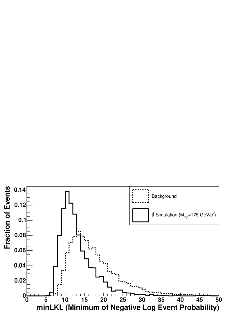
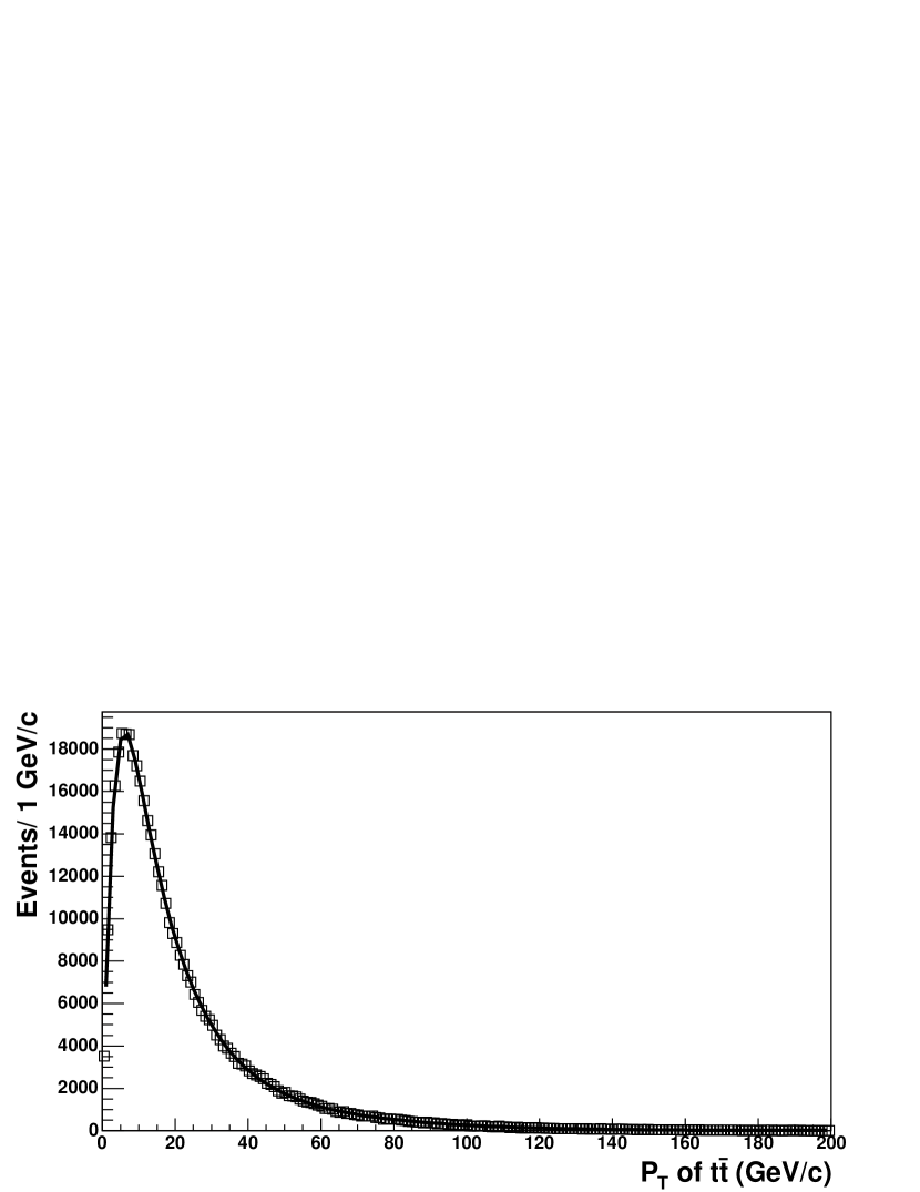
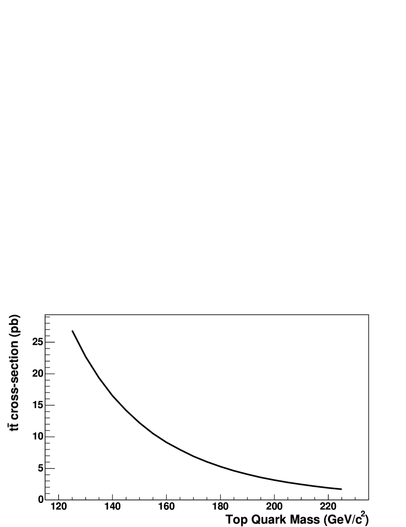

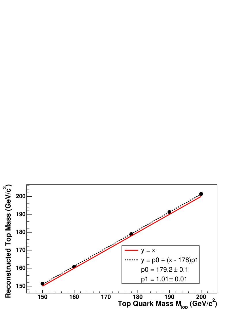
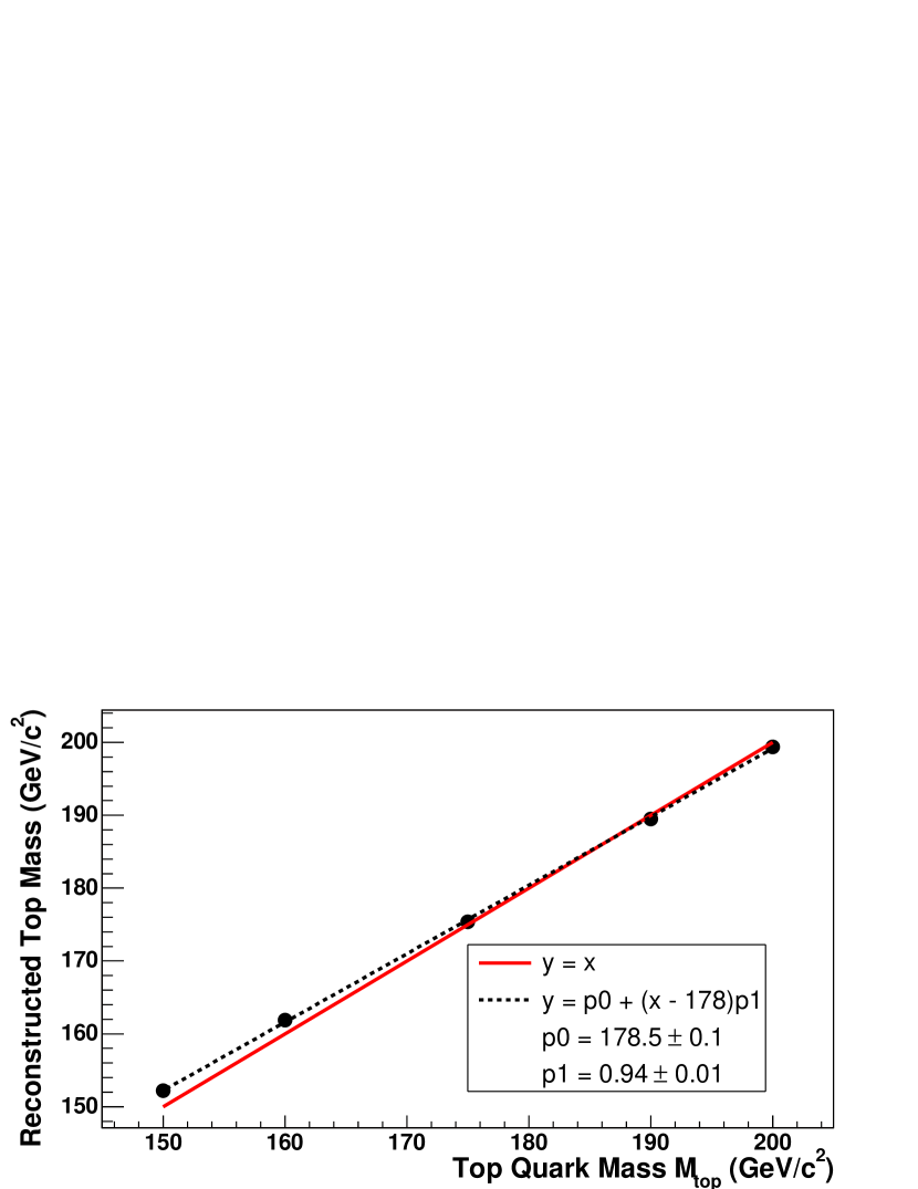
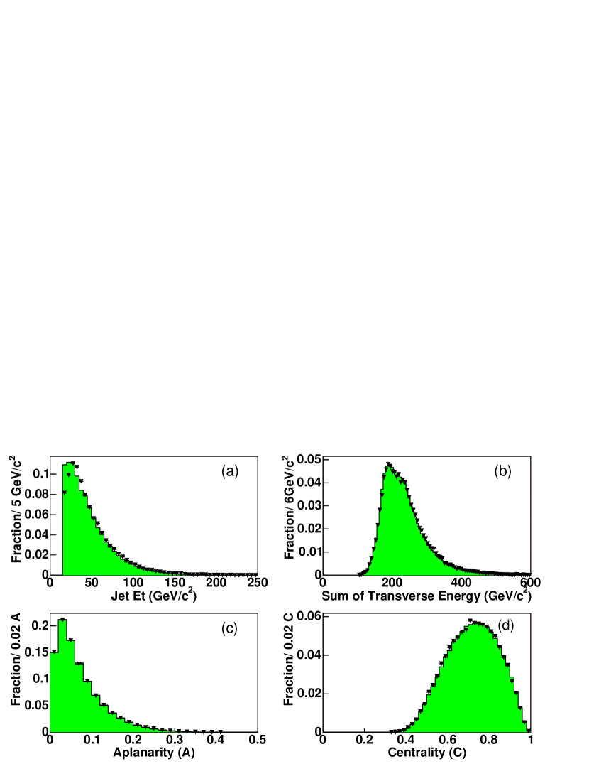
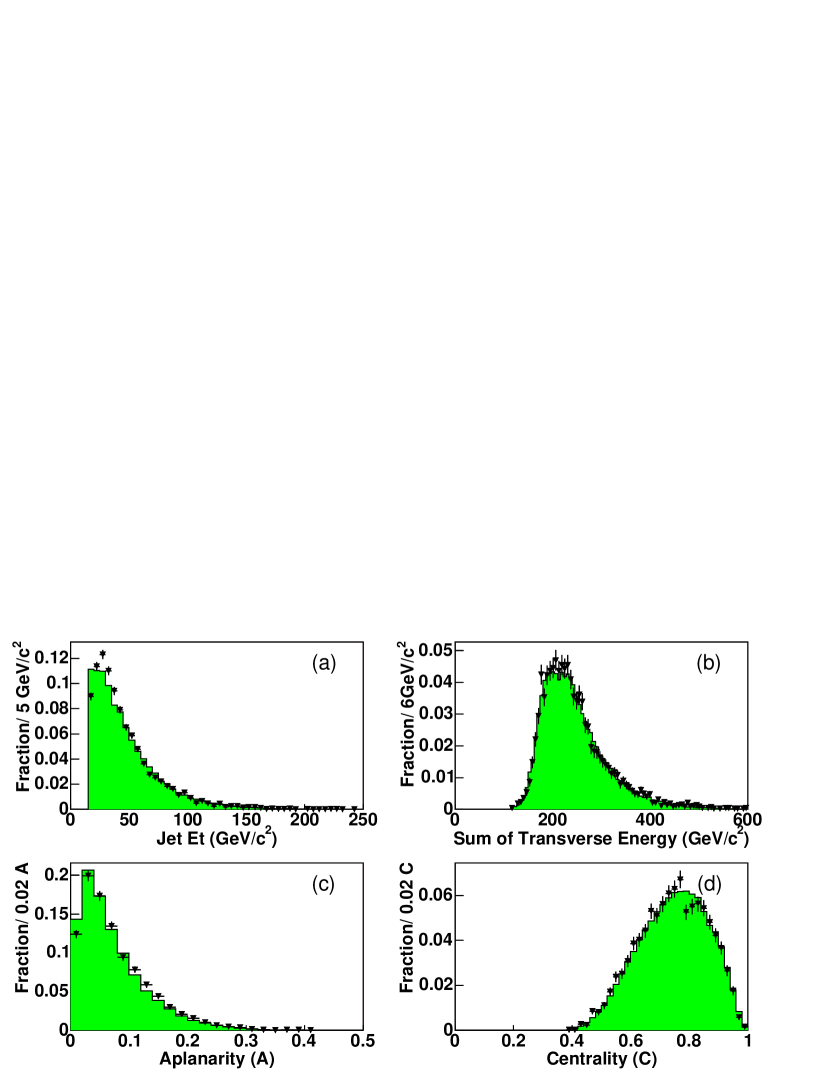
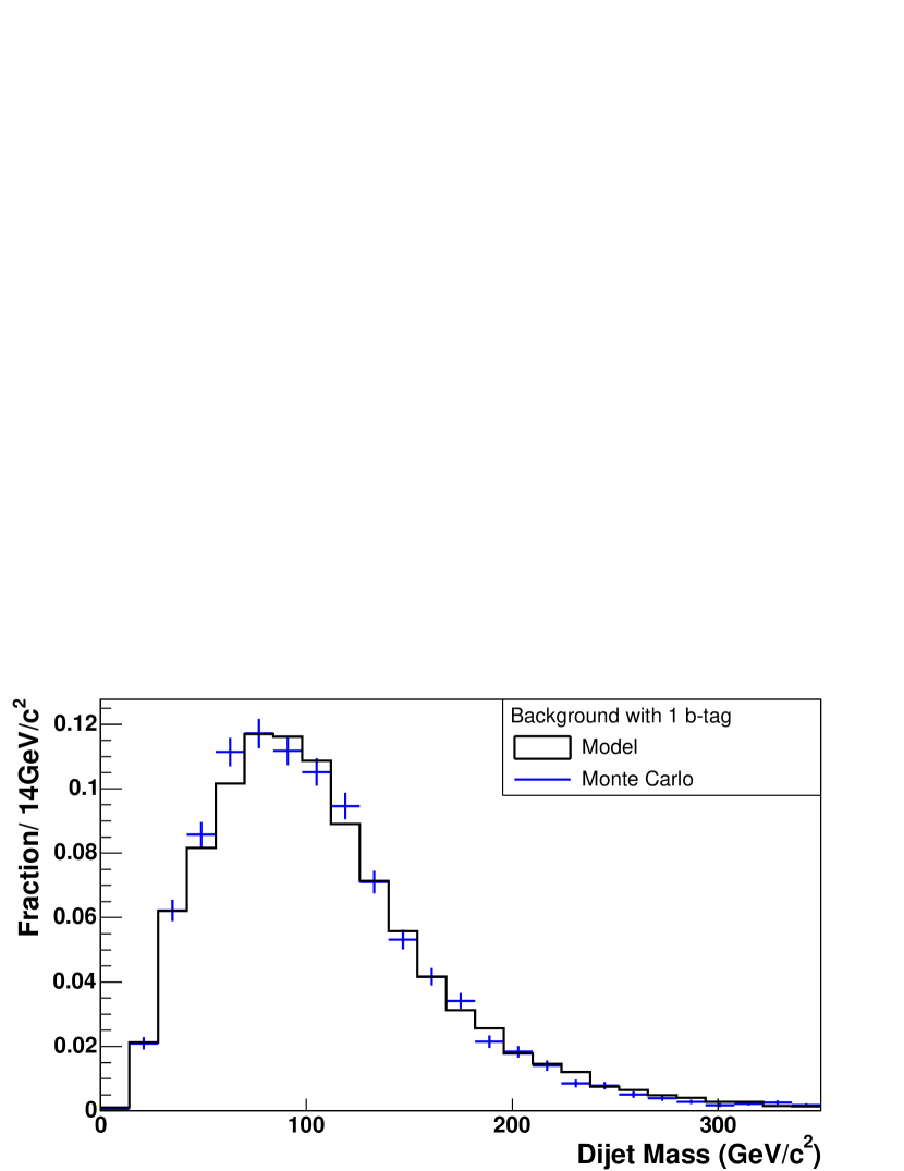 (b)
(b)
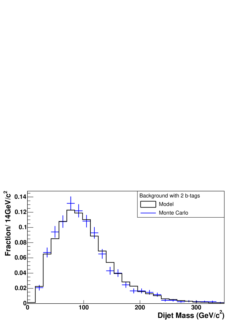
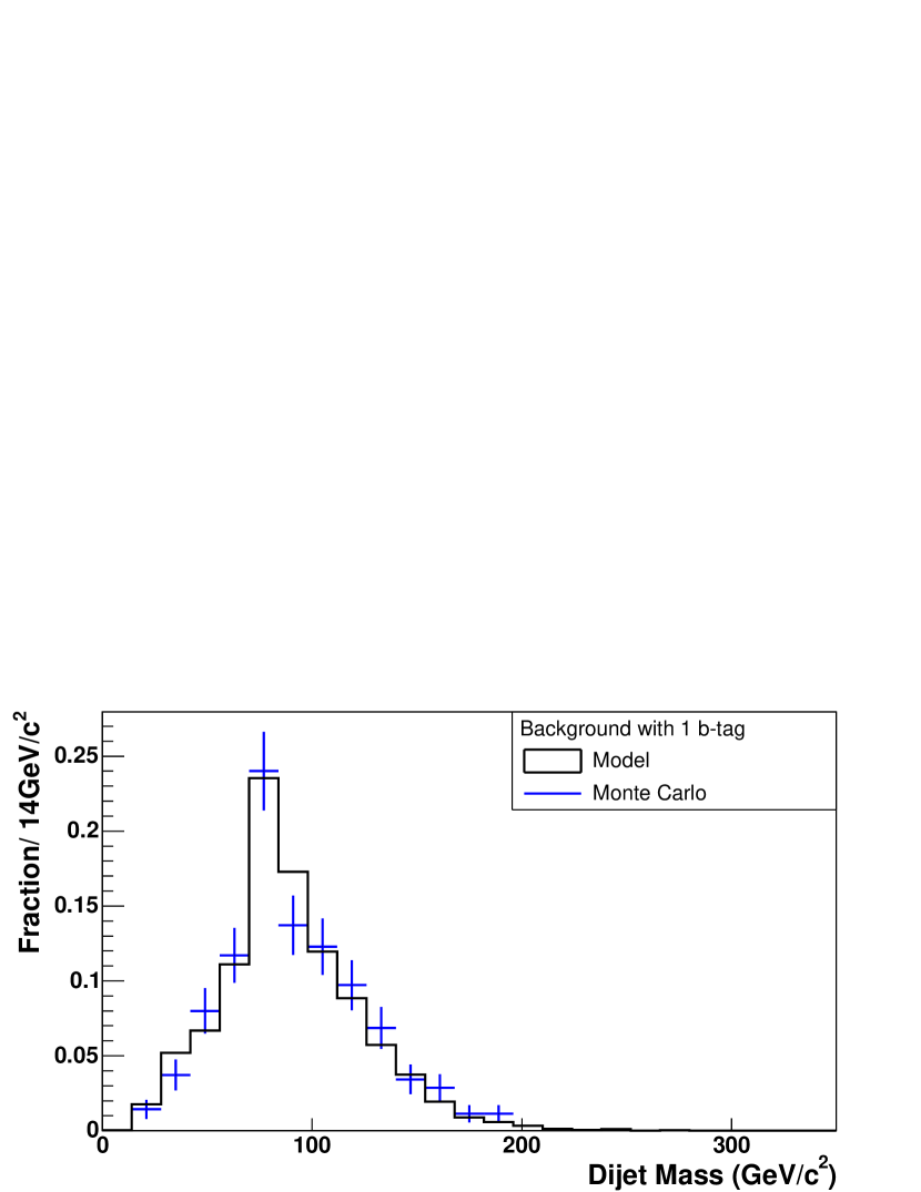 (b)
(b)
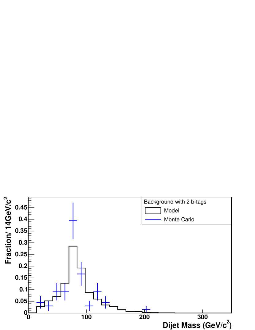
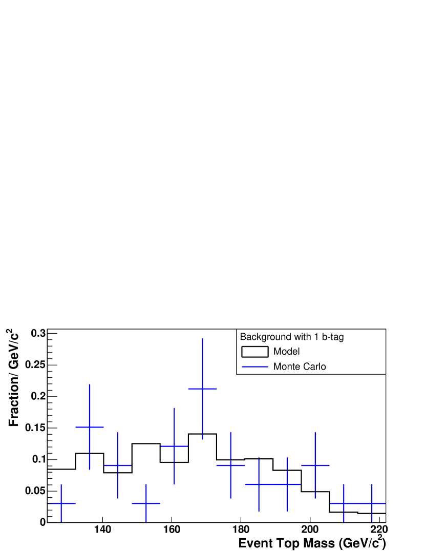 (b)
(b)
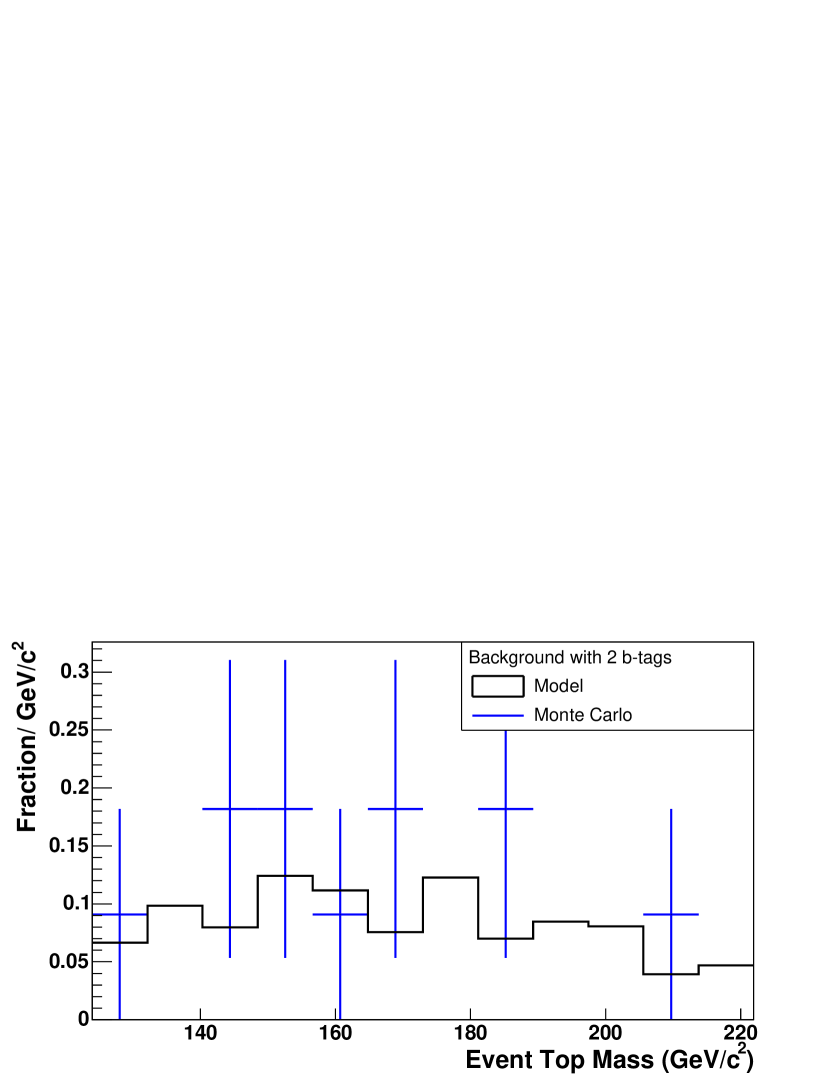
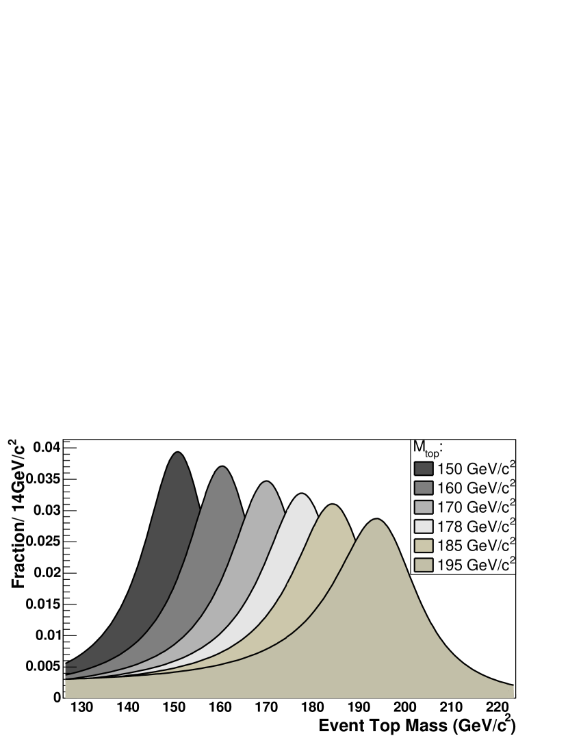
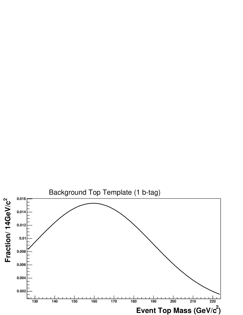 (b)
(b)
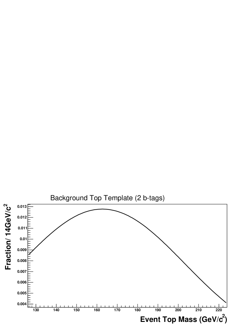
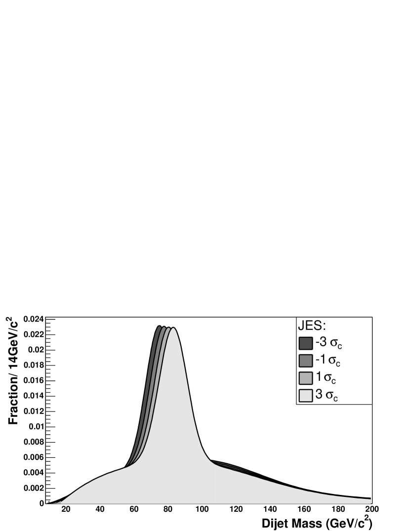
 (b)
(b)
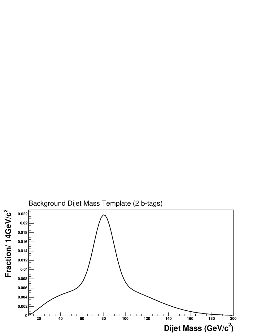
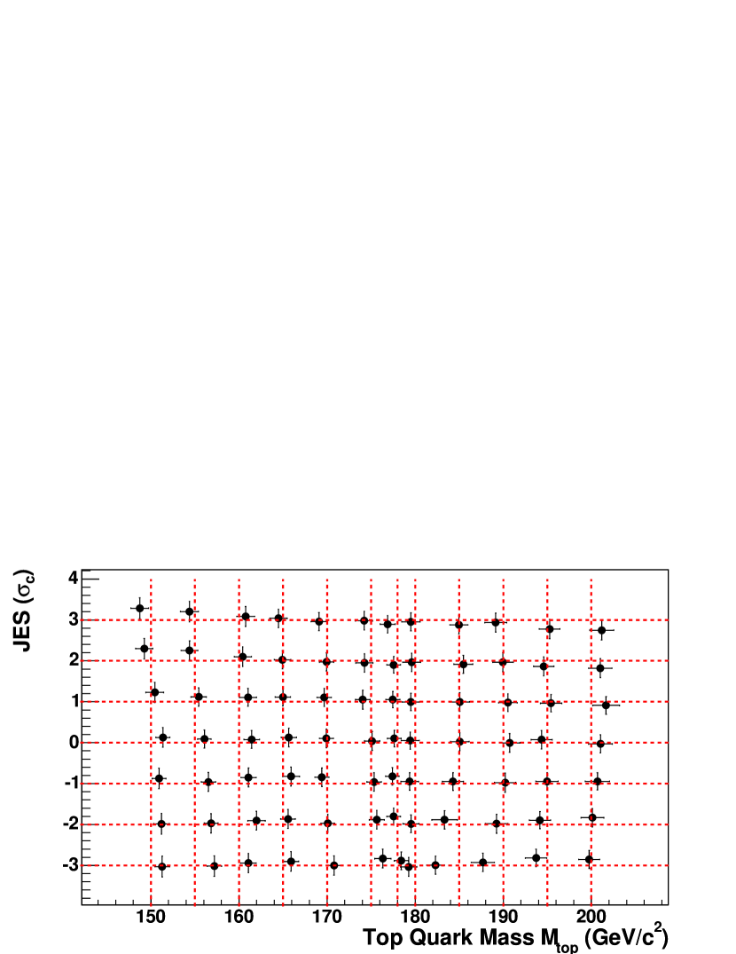
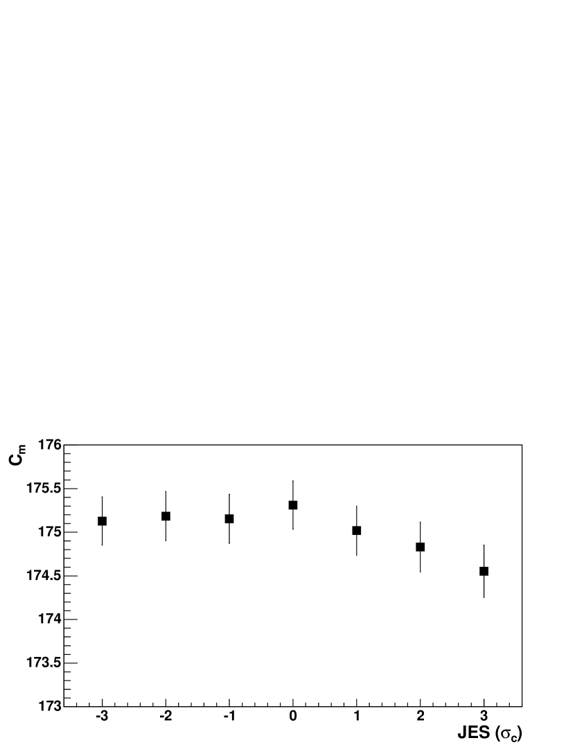
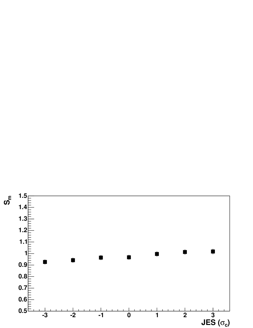
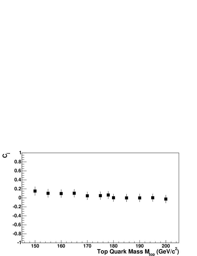

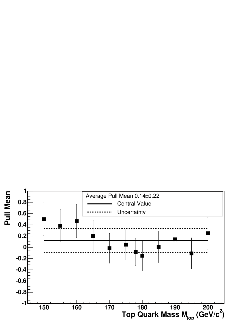
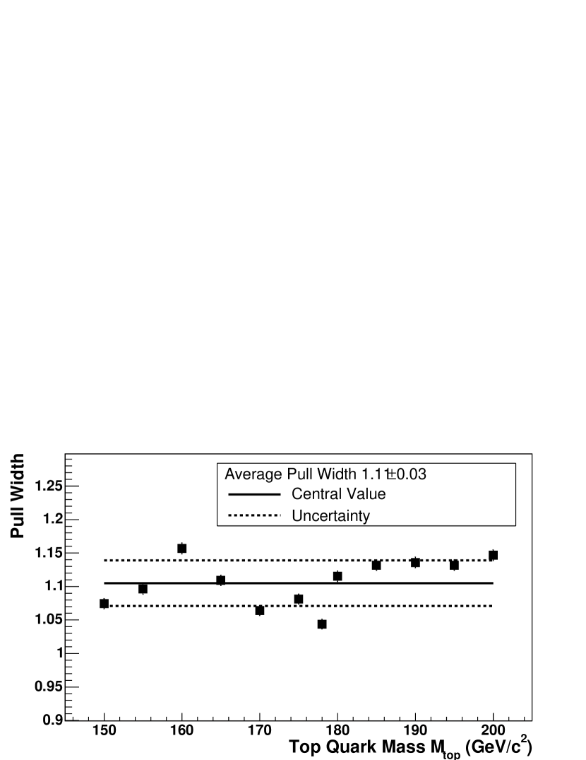
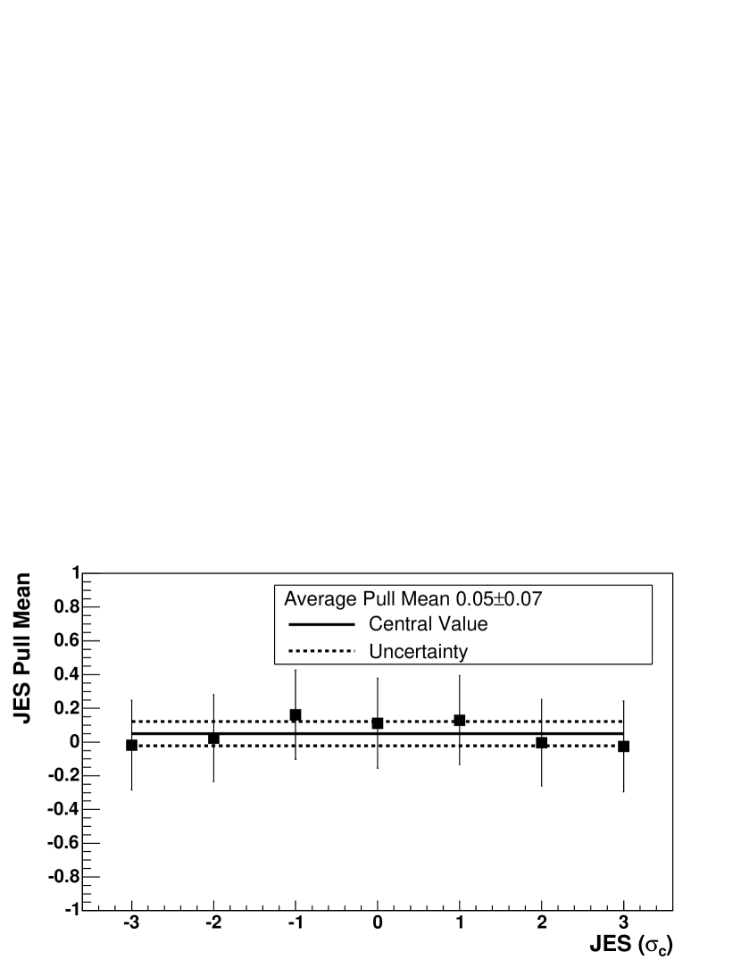
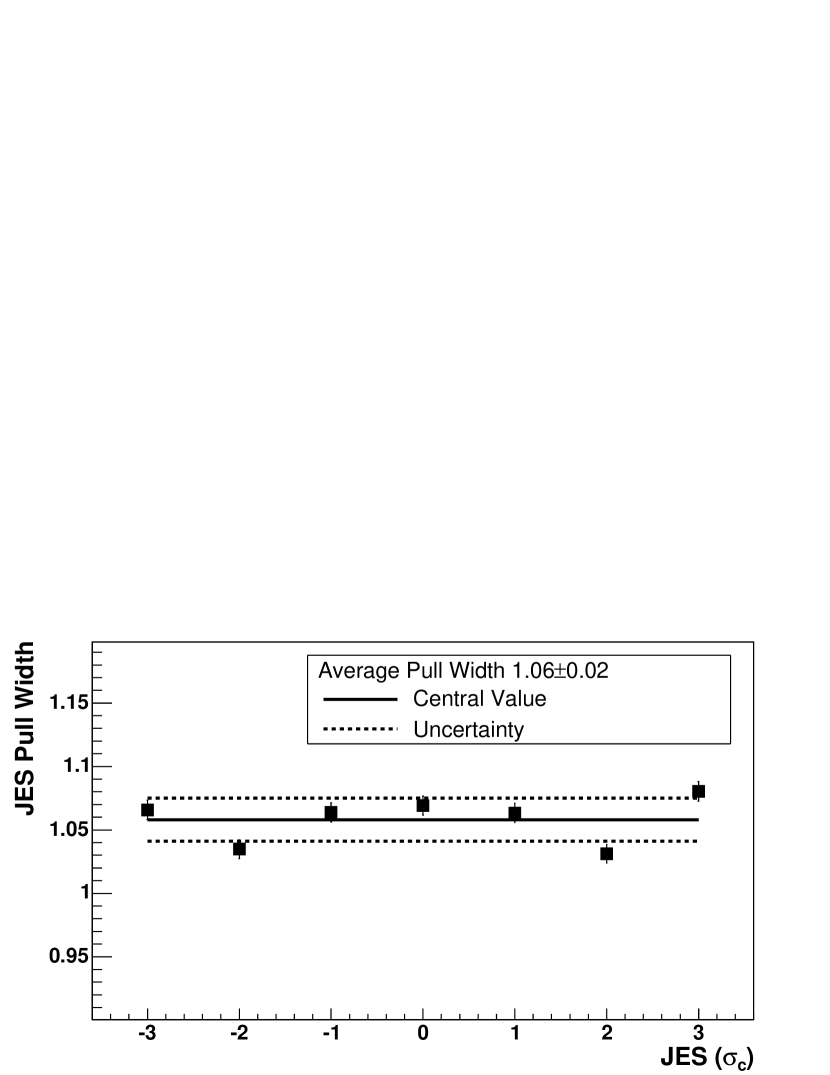
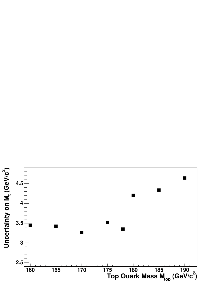
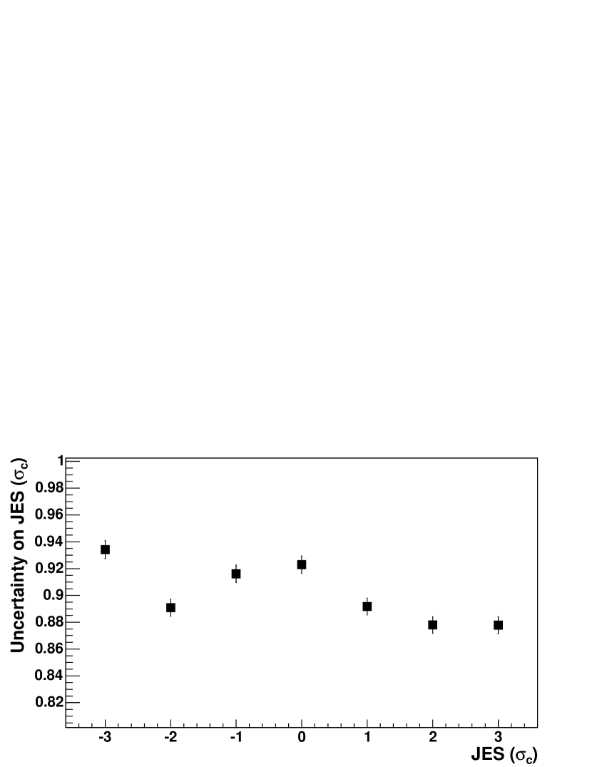
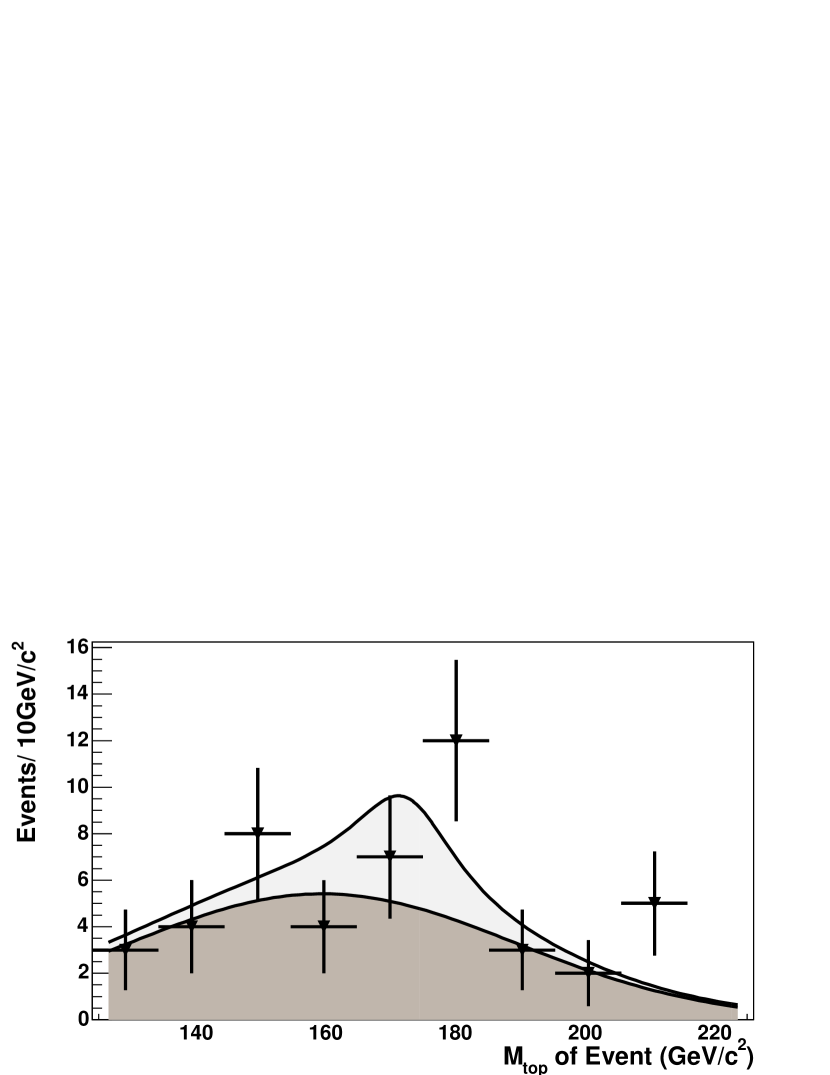 (b)
(b)