The Spitzer c2d Legacy Results: Star Formation Rates and Efficiencies; Evolution and Lifetimes
Abstract
The c2d Spitzer Legacy project obtained images and photometry with both IRAC and MIPS instruments for five large, nearby molecular clouds. Three of the clouds were also mapped in dust continuum emission at 1.1 mm, and optical spectroscopy has been obtained for some clouds. This paper combines information drawn from studies of individual clouds into a combined and updated statistical analysis of star formation rates and efficiencies, numbers and lifetimes for SED classes, and clustering properties. Current star formation efficiencies range from 3% to 6%; if star formation continues at current rates for 10 Myr, efficiencies could reach 15% to 30%. Star formation rates and rates per unit area vary from cloud to cloud; taken together, the five clouds are producing about 260 M⊙ of stars per Myr. The star formation surface density is more than an order of magnitude larger than would be predicted from the Kennicutt relation used in extragalactic studies, reflecting the fact that those relations apply to larger scales, where more diffuse matter is included in the gas surface density. Measured against the dense gas probed by the maps of dust continuum emission, the efficiencies are much higher, with stellar masses similar to masses of dense gas, and the current stock of dense cores would be exhausted in 1.8 Myr on average. Nonetheless, star formation is still slow compared to that expected in a free fall time, even in the dense cores. The derived lifetime for the Class I phase is 0.54 Myr, considerably longer than some estimates. Similarly, the lifetime for the Class 0 SED class, 0.16 Myr, with the notable exception of the Ophiuchus cloud, is longer than early estimates. If photometry is corrected for estimated extinction before calculating class indicators, the lifetimes drop to 0.44 Myr for Class I and to 0.10 for Class 0. These lifetimes assume a continuous flow through the Class II phase and should be considered median lifetimes or half-lives. Star formation is highly concentrated to regions of high extinction, and the youngest objects are very strongly associated with dense cores. The great majority (90%) of young stars lie within loose clusters with at least 35 members and a stellar density of 1 M⊙ pc-3. Accretion at the sound speed from an isothermal sphere over the lifetime derived for the Class I phase could build a star of about 0.25 M⊙, given an efficiency of 0.3. Building larger mass stars by using higher mass accretion rates could be problematic, as our data confirm and aggravate the “luminosity problem” for protostars. At a given , the values for are mostly less than predicted by standard infall models and scatter over several orders of magnitude. These results strongly suggest that accretion is time variable, with prolonged periods of very low accretion. Based on a very simple model and this sample of sources, half the mass of a star would be accreted during only 7% of the Class I lifetime, as represented by the eight most luminous objects.
1 Introduction
Star formation in the solar neighborhood has been studied extensively, but a complete survey for forming stars in nearby molecular clouds has been lacking. The IRAS catalogs provided an unbiased survey, but they were limited in sensitivity, wavelength coverage, and spatial resolution. For objects in embedded phases of evolution, the luminosity limit was about L⊙ with in pc (Myers et al., 1987). The wavelength coverage from 12 to 100 µm covered the peak of emission from typical Class I objects, but deeply embedded Class 0 sources were often missed, requiring special processing to be detected in IRAS data after being found at longer wavelengths (André et al., 2000). In addition, shorter wavelength data were needed to identify less embedded objects and to learn more about the embedded ones. Follow-up studies at shorter wavelengths often found multiple sources, which could be confused within the large beams of IRAS. Detailed studies in the mid-infrared from the ground were hampered by the atmosphere and limited to small regions already known to have luminous sources or clusters.
Ground-based near-infrared surveys, enabled by the development of large format near-infrared arrays, are a powerful tool for finding low luminosity YSOs in nearby clouds with relatively low extinction. High spatial resolution and sensitivity in these surveys decrease the level of confusion found in older surveys (e.g., Strom et al., 1989; Eiroa et al., 1992). Indeed, the 2MASS survey at , and has been used extensively to characterize the young star population and distribution in a number of clouds (e.g., Carpenter, 2000). Many of these studies have focused on young clusters in more massive star-forming regions, however (see review by Lada & Lada, 2003).
The Infrared Space Observatory (ISO) improved significantly on IRAS in terms of sensitivity and spatial resolution at the mid-infrared wavelengths. The ISOCAM instrument mapped a few square degrees of nearby star-forming clouds in two bands at 6.7 and 14.3 µm (e.g., Bontemps et al. 2001, Persi et al. 2003, Kaas et al. 2004). The mid-infrared observations revealed the more embedded population compared with near-infrared surveys. The number of Class II sources with L⊙ in Ophiuchus was doubled (Bontemps et al., 2001). These studies were focused on the densest parts of the clouds, but they clearly indicated the importance of deep mid-infrared observations.
The Spitzer mission, combined with ground-based near-infrared and submillimeter data, can remedy most of the deficiencies of previous studies. Spitzer can provide a survey that is deep, wide, and relatively unbiased, and that covers the entire wavelength range needed to characterize the different evolutionary stages, from deeply embedded YSOs to young stars which have lost most of their disks. Here we summarize the results of the Spitzer legacy project, “From Molecular Cores to Planet-forming Disks”, or “Cores to Disks”, further abbreviated to c2d (Evans et al., 2003). One of the main approaches of the c2d project has been to provide a more complete, less biased sample of star formation in nearby large clouds and small cores. Toward that end, we used Spitzer to map 15.5 square degrees in five large, nearby molecular clouds and about 0.6 square degrees in 82 small dense cores. For this paper, we focus on the studies of large clouds, where the mapping efficiency of Spitzer enables coverage of large areas, in contrast to previous surveys, which focused on small areas around IRAS sources, for example. The results on the small cores will be summarized by Huard et al. (2008).
Based on all of our data and some auxiliary data, we construct a combined list of young stellar or substellar objects (hereafter YSOs). We discuss issues of contamination and completeness, and we calculate various quantities that will be used in the analysis (§3). We summarize the star formation efficiencies and rates (§4), comparing our results to predictions used in extragalactic work (§4.1). These values supercede preliminary values (Evans et al., 2008). We compare numbers of sources in various SED classes and calculate lifetimes for these classes (§5). We then reexamine the issues of source classification (§6), the connection between empirical classes and various stages of star formation, and the estimation of lifetimes for these stages (§7). We discuss the spatial distribution of sources and their clustering properties (§8). Finally, we compare the observational results to the predictions of various theoretical models (§9), describe future work (§10), and summarize the main results (§11).
1.1 The Sample
Five large clouds were selected for the c2d project: Serpens (Eiroa et al., 2008), Perseus (Bally et al., 2008), Ophiuchus (Wilking et al., 2008), Lupus (Comerón, 2008), and Chamaeleon (Luhman, 2008). More specifically, we targeted Lupus I, III, and IV and Chamaeleon II (hereafter Cha II). These were chosen to lie within about 300 pc of the Sun, to span a range of previously-known star formation activity, and to complement observations of smaller regions in these clouds obtained by Guaranteed Time Observers (GTOs). We have included data from the GTO observations with our data for a complete picture of the clouds.
The clouds in this study are listed in Table 1, with the adopted distances, solid angles and areas with both IRAC and MIPS data, a measure of turbulence, the total mass in the mapped area, and the crossing time. Some of these clouds were targets of ISO surveys of smaller regions: 0.7 sq. deg. in Ophiuchus (Bontemps et al., 2001); 0.13 sq. deg. in Serpens (Kaas et al., 2004); and 0.2 sq. deg. in Cha II (Persi et al., 2003). The results presented here are based on detailed studies of the individual clouds: Serpens (Harvey et al. 2006; Harvey et al. 2007; Harvey et al. 2007b); Perseus (Jørgensen et al. 2006; Rebull et al. 2007; Lai et al. 2008); Ophiuchus (Padgett et al. 2008b; Allen et al. 2008b); Lupus (Chapman et al. 2007; Merín et al. 2008a); and Cha II (Young et al. 2005; Porras et al. 2007; Alcalá et al. 2008; Spezzi et al. 2007; Spezzi et al. 2008). Numbers in those papers have been updated based on a consistent analysis of the combined dataset.
None of these clouds are forming very massive stars; the most massive star in the close vicinity of a cloud mapped by c2d is HD147889, a B2 (III/IV) star lying within our map of Ophiuchus. The Sco group is farther away (projected distance from the cloud of 4 pc), consisting of an O9V star and a B2III star and at least two other B stars (Pigulski, 1992). The star formation patterns in Ophiuchus may have been affected by interaction with these stars (Loren 1989, Nutter et al. 2006). For Perseus, there are hints of an interaction with 40 Per, a B0.5 star in the Per OB Association, which is 26 pc from the L1451 core, as discussed by Walawender et al. (2004) and Kirk et al. (2006). Serpens contains a Herbig Ae star, VV Ser, which produces a large nebulosity (green object toward the south in Figure 1) discussed by Pontoppidan et al. (2007a) and Pontoppidan et al. (2007b). In addition, Serpens contain 3 other A-type stars and a B8 star (Oliveira et al., 2008). The most massive star in the Cha II cloud is the F-type star DK Cha (Hughes & Hartigan, 1992); all the rest have spectral type later than K2 (Spezzi et al., 2008). The Lupus clouds are in the vicinity of the Scorpius-Centaurus association, which flanks the Lupus clouds at a distance of about 5 degrees, or 17 pc at a distance of 200 pc. The sub-groups of the association are called Upper Scorpius (5-6 Myrs) and Upper Centaurus-Lupus (14 Myrs) (de Geus et al., 1989). The strong high-energy radiation and supernova remnants from those OB stars might have had an important role in the formation and evolution of the Lupus clouds (Tachihara et al., 2001). Specificially, the highly fragmented cloud structure is thought to be related to the effects of the nearby OB association.
There are distance uncertainties for all five clouds, which are discussed in the detailed papers on those clouds. Here we supply our adopted uncertainties and propagate those into the areas and masses. Recent parallax observations of radio emission from young stars in Ophiuchus yield a distance of pc (Loinard et al., 2008). By combining extinction maps with parallaxes from Hipparcos and Tycho, Mamajek (2008) found a distance of pc, while Lombardi et al. (2008) have derived a distance of pc. These are all consistent with our assumed distance and uncertainty of pc. Because it is not clear that the whole cloud is at the same distance (Loinard et al. 2008, Lombardi et al. 2008), we retain our value and uncertainty in the analysis. A recent astrometric measurement of water masers in NGC1333, in Perseus, provides a distance of pc (Hirota et al., 2008). Distance estimates for IC348 are larger, so we retain our standard distance and uncertainty of for the Perseus cloud as a whole. Lombardi et al. (2008) also derived a distance to the Lupus complex of pc, with some evidence that individual Lupus clouds were at different distances, both consistent with our assumed values of pc for Lupus I and IV and pc for Lupus III. We use a distance to Serpens of pc (Straizys et al., 1996), as was used in all our previous papers on this cloud, but we note that there is some recent evidence for a distance of pc (Eiroa et al., 2008).
Seeking a common measure of the turbulence of these clouds, we chose to give the FWHM linewidth of the 13CO line, ideally averaged over a full map of the cloud. This was not available in all cases, so we have resorted to accepting statements like “a typical linewidth is …” (Hara et al., 1999) for Lupus. For Perseus, Serpens, and Ophiuchus, J. E. Pineda (pers. comm. 2008) has provided the mean and median linewidths for the ensemble of spectra in the COMPLETE maps (Ridge et al., 2006), and the average and difference of the median and mean are given in Table 1 as the value and uncertainty. Tothill et al. (2008) have provided the same kind of information for the line of 13CO in Lupus, based on maps with AST/RO. The linewidths are based on dividing the integrated intensity by the peak intensity and correcting for the channel width of 0.91 km s-1, assuming Gaussian lines. The results are substantially larger than the estimates from the 13CO lines. For Lupus I, ; for Lupus III, ; and for Lupus IV . It would be valuable to have more consistent and sophisticated measures of the turbulence in these clouds.
The cloud mass (gas and dust) has been derived from extinction maps made from our c2d data, together with 2MASS data, toward background stars (Evans et al., 2007). We used the extinction law with (Weingartner & Draine, 2001), which reproduces reasonably well the data for molecular clouds (Flaherty et al. 2007; Chapman et al. 2009), to determine . The mass was then calculated using the relation (Draine, 2003) and the value of from the on-line tables111Available at http://www.astro.princeton.edu/ draine/dust/dust.html for . This grain model results in a conversion from extinction to hydrogen column density of 1.37 cm-2 mag-1, instead of the usual 1.87, established for diffuse ISM gas (Bohlin et al., 1978). In our earlier papers (Harvey et al. 2007b, Alcalá et al. 2008, Chapman et al. 2007, Merín et al. 2008a), the value for the diffuse gas was used, resulting in cloud masses overestimated by a factor of 1.4 relative to those in Table 1.
The mass includes all cloud mass above an extinction contour with mag, with no assumptions needed about geometry. The mass derived from our extinction maps refers to the same area covered in our surveys, making it ideal for calculations of efficiency, etc. The two exceptions to this statement are Serpens, for which our survey was designed to cover completely down to , and Ophiuchus, for which we tried to cover completely down to . The coverages were based on extinction maps by Cambrésy (1999), but some areas down to were covered incompletely. The mass inside the contour for Serpens is 1532 M⊙, 76% of the mass within . The mass inside the contour for Ophiuchus is 1914 M⊙, 88% of the mass within . We use the value for in what follows, but the difference will not be large for these clouds. Table 1 also gives the cloud crossing time in Myr, calculated from the area and the mean speed of turbulent motions, approximated by , with the 13CO linewidth.
With the sensitivity of Spitzer, we can detect sources with luminosity as low as L⊙ at 350 pc, but contamination by other kinds of sources ultimately limits our sensitivity, as discussed below. A similar study of the Taurus cloud has been done by Padgett et al. (2008a), and other clouds in the Gould Belt are being mapped with the same techniques (Allen et al., 2008a). When those studies are completed, the analysis in this paper can be extended to cover most star formation in large clouds within about 300 pc of the Sun.
2 Observations
The observations here were all obtained by the c2d project or by GTO observations that we have included in our data. They have been described in the publications given in §1.1. Here, we give a brief summary of the data used for this paper; a more complete description can be found in Evans et al. (2007).
The Spitzer instruments were used to obtain data from 3.6 to 160 µm, but the 160 µm data are limited by saturation, incomplete coverage, and the large beam. Photometry at 160 µm is not available as a standard product in the c2d catalogs. We provide and use some limited photometry at 160 µm here. Data from the four IRAC bands (3.6, 4.5, 5.6, and 8.0 µm) and data from the 2 µm All Sky Survey (2MASS) (Cutri et al., 2003) were merged using a 2″ matching radius. These sources were merged with photometry from MIPS at 24 µm (4″ radius). The 70 µm data were merged with an 8″ radius, but human judgment was used when multiple candidates for merging were available at the shorter wavelengths. The merging of IRAC and MIPS data could be done only for the area covered by both IRAC and MIPS observations, and larger areas were usually covered by MIPS observations. Since we use data from both instruments to separate YSOs from other sources, we focus here on the areas with both IRAC and MIPS data.
For one cloud (Cha II), optical photometry has also been published (Spezzi et al., 2007). Also for Cha II and Serpens, we have reasonably complete spectral type information (Spezzi et al. 2008 and Oliveira et al. 2008). For three clouds (Perseus, Ophiuchus, and Serpens), complete maps of dust continuum emission at 1.1 mm were made using Bolocam on the Caltech Submillimeter Observatory. These have been published (Enoch et al. 2006, Young et al. 2006, Enoch et al. 2007) and the Bolocam data have been combined with Spitzer data (Enoch et al. 2008a, Enoch et al. 2008b). We will draw on those results here. We also have less sensitive maps of 1.3 mm emission for Cha II (Young et al., 2005) and maps of selected regions at 350 µm (Wu et al., 2007). Maps of emission from the transitions of CO and 13CO were obtained by the COMPLETE project for Perseus, Ophiuchus, and Serpens (Ridge et al., 2006). Maps of the line of 13CO were obtained for Lupus and Cha II by Tothill et al. (2008).
3 Results
Figure 1 presents three color images of all the clouds on the same physical scale, with a 3 pc scale bar. Figure 2 shows the extinction in grayscale, with all clouds on the same physical scale and extinction grayscale. All the identified YSOs are shown, color-coded by their SED class (§5.1). The total area covered is dominated by Perseus, Ophiuchus, and Serpens.
Tables 8 to 12 are described in the Appendix. They are electronic tables providing a full list of YSOs in the five clouds, based on an updated, uniform analysis of the entire sample, using the final data release from the c2d project222Available at http://ssc.spitzer.caltech.edu/legacy/c2dhistory.html with a thorough description (Evans et al., 2007). The information in the tables in this paper is a condensed version of that found in the full c2d catalogs, along with supplementary information. Briefly, the c2d catalogs provide flux densities, uncertainties, and various flags for each wavelength from 3.6 to 70 µm, similar information for the 2MASS sources that match our sources, a source type, and a spectral index. Since the source type plays an important role in discussing contamination, we briefly summarize the nomenclature here.
Only sources with detections in at least three bands could be classified at all. If an object was consistent with a (possibly reddened) stellar photosphere, it was labeled “star”. Candidates for YSOs required detections in all four IRAC bands and MIPS-1; those meeting stringent criteria (see 3.1) are labeled YSOc, with the “c” emphasizing that they are only candidates. They may have one or more appended suffixes, such as “red”, “PAH_em”, or “stardust”. Sources labeled “red” have flux densities at 24 µm that are at least three times the flux density from the nearest available IRAC band. Sources labeled “PAH_em” have colors indicative of a peak in the 8 µm band. The “stardust” designation indicates that the SED is consistent with that of a stellar photosphere for wavelengths shorter than a particular band but an excess in that band of at least 3 . This band was appended to make a full name such as “YSOc_stardust(MP1)” where MP1 implies the first MIPS band, at 24 µm. As discussed below, some sources lacked photometry at enough wavelengths to be classified as YSOc, but were later added as YSOs based on other information. These may have source types in Table 12 of “rising”, in which the available flux densities rise significantly to longer wavelengths (15 cases), or “red1”, in which the source is detected only in IRAC-4 or MIPS-1 (3 cases).
In this paper, we refine and standardize the analysis of the combined data for the five large clouds, discussing issues of contamination by background sources (§3.1) and completeness (§3.2). After describing the standard classification tools provided in the catalogs, we describe analysis that goes beyond that provided in the catalog. We discuss extinction corrections (§3.3) that can be be made to the flux densities and the calculation of bolometric luminosity () and bolometric temperature (). We present in the Appendix the list of YSOs, including flux densities from 2MASS ( m) and Spitzer ( m). Additional flux densities from observations with other telescopes, at wavelengths ranging from 0.36 m to 1.3 mm, are presented in Tables 8, 9, 10, and 11. This list of YSOs is improved over the list of YSOc supplied with our delivery because we have removed some suspect sources, added known sources, added data at other wavelengths, and calculated additional quantities, provided in Table 12. We describe this process in the following subsections.
3.1 Contamination by Other Sources
The main challenge is to separate YSOs from contaminants. By far, most contaminants are stars, mostly background, without infrared excess. These have colors very close to zero in a color-color diagram using the IRAC bands (Allen et al., 2004) and are easily removed. The primary remaining contaminants are then background galaxies with active star formation; these may have colors very similar to those of embedded young objects, so we must use magnitude information as well as colors.
The automated criteria described by Harvey et al. (2007b) were used for all five clouds to produce catalogs of YSO candidates (YSOc), which are part of our final data delivery. Compared to earlier catalogs, advances in distinguishing YSOs from background galaxies (Harvey et al., 2007b) have provided much cleaner samples. These criteria assign to each source with sufficient information an unnormalized probability () that the source is a galaxy. The calculation of the probability is complex and fully described in Harvey et al. (2007b) and Evans et al. (2007), so we summarize it here. The probability depends on the location of the source in three color-magnitude diagrams, whether the source is extended, and whether the source is detected above a threshold at 70 µm. The assignment of probabilities is entirely empirical, based on excluding objects in a suitable sample of extragalactic observations.
By comparing to a set of sources from the SWIRE survey of the ELAIS N1 extragalactic field (Surace et al., 2004), suitably processed to simulate the c2d sensitivity and the extinction distribution of each cloud, we define a threshold in below which a source becomes a YSOc. For the catalogs of the five large clouds, the aggregate plot is shown in Figure 3. As was true for the individual clouds, most YSOc separate nicely from galaxy candidates (Galc), but there are some sources in a lower probability tail from the big peak in the Galc sector that are ambiguous. Thus, confusion with star-forming galaxies can be a problem for both contamination and completeness. Sources with log were assigned the YSOc moniker in the c2d catalogs, based on the analysis of Serpens by Harvey et al. (2007b). From the surface density of objects from the degraded SWIRE data that would be misclassified as YSOc for each cloud, multiplied by the surface area of the cloud, we estimate that there could be as many as 51 contaminating galaxies in our total 15.5 square degrees. That would still be a small fraction of the total of 1086 YSOc (see below). We next describe attempts to minimize the number of contaminants.
Certain categories of sources were checked by eye for all the clouds in an attempt to eliminate residual contaminants. Typically these were sources that had been “band-filled” at 24 µm or sources with peculiar SEDs. Sources that were well detected at some wavelengths received flux estimates at other wavelengths, based on the known position, in the process of band-filling. Some of these flux estimates turned out to be emission from the wings of nearby bright sources and other artifacts. In addition, objects with the “PAH_em” suffix received extra scrutiny because this feature is common in star-forming galaxies. Objects that had galactic morphologies were removed from the final YSO list; however, many star-forming galaxies are point-like to Spitzer. A total of 91 YSOc were eliminated by this process. We do not know how many point-like galaxies were removed by this process, but the numbers are consistent with removing most of them.
While stars without infrared excess are readily removed from our sample via color criteria, post-main-sequence stars with circumstellar shells can masquerade as YSOs. Harvey et al. (2007b) were able to identify and remove 4 of these behind the Serpens cloud. Follow-up optical spectroscopy toward Serpens (Oliveira et al., 2008) have provided spectral types for 78 objects, 58 of which had been identified as YSOs. Based on their analysis, we rejected 11 of those 58 sources (about 20%) as background giants with infrared excesses (Oliveira et al., 2008). All 11 are classified as either Class II or Class III sources, with 9 out of 11 (about 80%) classified as Class III. We have removed these 11 sources from the final sample. We so far lack the data required to identify and remove background giants in Lupus, Perseus, and Ophiuchus. However, Serpens should be the worst case because it lies at low galactic latitude and longitude. Lupus and Ophiuchus may also be affected, though less so than Serpens. Additionally, a spectroscopic study of Cha II found that 96% of the YSOs identified in our catalogs were true cloud members (Spezzi et al., 2008). These points, combined with the fact that most of the background giants (80%) are Class III sources, to which we are incomplete anyway (§3.2), lead us to conclude that contamination by background giants will not significantly affect our main results.
Adding these 11 background giants in Serpens to the 91 sources removed as described above gives a total of 102 sources removed from the initial sample of 1086 YSOc (Table 2).
3.2 Completeness
Since the vast majority of sources in the catalogs are background stars, we require an infrared excess for a source to be considered a candidate YSO. Consequently, our sample is missing Pre-Main-Sequence Stars (PMS) that no longer have infrared excess but may have H emission, X-ray emission, etc. Complete surveys for such objects are needed to complete the sample of PMS objects, so we concentrate on YSOs, defined here to have an infrared excess. More complete samples of PMS objects exist for some clouds that have the needed complementary data, but not for all. For example, Alcalá et al. (2008) found 51 certain and 62 likely PMS stars in Cha II, more than double the number (26) of YSOs. The ratio of PMS to YSOs in our catalog is 2 for Class II sources and 4.8 for Class III sources. Cha II may be a worst case because many of the PMS stars are not in the region studied by c2d. Restricting attention to that region, only 4 PMS stars are added to the YSOs found by c2d. A similar study in Lupus would add 19 PMS stars without infrared excess to the 94 YSOs (Merín et al., 2008a).
While objects of very low luminosity may still be lost among the galaxy background, we estimate that our YSO sample is 90% complete down to a luminosity integrated from 1 to 30 µm of 0.05 L⊙ and 50% complete down to 0.01 L⊙ (Harvey et al., 2007b) for our most distant cloud (Serpens at 260 pc, which also has the highest density of background stars). For comparison, the survey of Serpens with ISO reached a limit of 0.08 L⊙, but had only two bands and covered only 0.13 sq. deg. (Kaas et al., 2004). They found 61 YSOs compared to our 227, mostly because of their smaller areal coverage. The 1-30 µm wavelength range covers the bulk of emission from YSOs with infrared excesses arising from circumstellar disks; thus these completeness limits are a good proxy for our completeness to such objects. A 2 Myr old object at the mass boundary between stars and brown dwarfs has a luminosity of about 0.01 L⊙. Indeed some objects believed to be brown dwarfs with disks based on more complete analysis do not make our YSOc list, either because their fluxes are not of high enough quality or because they have log. For example, 2 of the 4 added PMS objects in Cha II are very low mass brown dwarfs with excesses (Allers et al., 2007).
For younger YSOs still embedded within their dense cores, this µm wavelength range is less appropriate since the bulk of the emission is reprocessed by the surrounding envelope to the far-infrared. A separate search for embedded objects with luminosities less than 1 L⊙ found that we reach a similar completeness limit for the internal luminosity of these objects ( of L⊙ at 140 pc, or L⊙ at 260 pc) (Dunham et al., 2008), where this limit is set by the sensitivity of the 70 µm MIPS-2 observations. The internal luminosity measures the contribution from the embedded source, after correction for the effects of heating by the interstellar radiation field.
We require good quality detections in all 4 IRAC bands and MIPS-1 for a source to be classified as a YSOc. This requirement can result in our missing two types of sources: deeply embedded sources that were not detected in all bands and strong sources that saturated the detectors. Note that the latter can include both embedded objects and more evolved YSOs no longer embedded within their dense cores. A total of 40 sources that are clearly YSOs but which did not make the automatically-generated YSOc list for one of the two above reasons were added by hand to our final sample, bringing the final sample size to 1024.
Of these 40 sources, 36 were added by comparison to the searches for embedded objects presented by Dunham et al. (2008), Enoch et al. (2008a), Jørgensen et al. (2007), and Jørgensen et al. (2008). Two were added by being well-known YSOs that were saturated in one or more of the Spitzer bands but not included in the samples of embedded objects compiled by the above authors. For all saturated sources, data from other telescopes were substituted for the saturated Spitzer data. Three of the added sources actually have source types of Galc, one each in Lupus, Perseus, and Serpens. The source in Lupus was added by Merín et al. (2008a) because it lies essentially on the border between YSOc and Galc, and it is candidate to be a brown dwarf with a disk (Allers et al., 2006). The source in Perseus was added because it is contained in the sample of embedded objects compiled by Jørgensen et al. (2007). The Serpens source is associated with an outflow.
Turning the luminosity completeness limit into a limit on stellar mass requires further analysis. For the early, embedded stages, the luminosity depends on the product of stellar mass and mass accretion rate. As discussed in §9.2, accretion at the mean rate expected in a Shu-type model would predict a luminosity of 1.6 L⊙ for a central object of 0.08 M⊙. Our luminosity limit of 0.014 L⊙ would then translate into a mass limit of 7 M⊙. However, there is strong evidence for highly variable accretion rates (§9.2), so this limit is highly suspect. For the later stages when accretion luminosity is negligible, spectral types and accurate extinction corrections are necessary to determine masses. For the most distant cloud (Serpens), a main-sequence luminosity of 0.05 L⊙ implies a mass of 0.08 M⊙, while 0.01 L⊙ correponds to 0.04 M⊙ (Chabrier et al., 2000). At young ages, the mass limits would be lower. In Serpens, the masses determined by Oliveira et al. (2008) from spectral types range from 0.2 to 3.0 M⊙. In Lupus, masses of YSOs are complete down to 0.1 M⊙ (Merín et al., 2008a), and in Cha II, masses extend well below the stellar limit to 0.015 M⊙ (Spezzi et al., 2008). We do clearly miss some substellar objects with disks, as discussed above. Until spectroscopy is available for a larger fraction of the young objects, we can only estimate our mass completeness to be near the stellar/substellar boundary.
3.3 Classification
For each source with sufficient data, the c2d catalogs provide a least squares fit to all photometry between 2 µm and 24 µm in the c2d catalog to determine the spectral index :
| (1) |
where is the wavelength and ) is the flux density at that wavelength. These were used to classify objects into the four classes defined by Greene et al. (1994), as described in detail in §5.1: Class I, Flat, Class II, and Class III.
An alternative classification scheme, used especially for more embedded objects, employs the bolometric temperature (). We will also need the bolometric luminosity () for later analysis. These were computed, using both Spitzer data and auxiliary data at both shorter and longer wavelengths, by calculating the first two moments of the SED (Chen et al., 1995) using integration methods described in more detail by Dunham et al. (2008). Uncertainties in and are dominated for early phases by incomplete sampling of the SED at wavelengths from 70 to 1000 µm; they were estimated to be 20 to 60% (Enoch et al. 2008a, Dunham et al. 2008). The poor sampling at far-infrared wavelengths arises in part because of the large beam of Spitzer, causing confusion in crowded regions, and from the lack of data at 350 µm. A recent analysis of the Serpens B cluster using the fine-scale 70 µm mode and adding 350 µm data (Harvey & Dunham, 2009) was able to separate sources that were confused in the c2d data. They find that the values of and change by about the amount estimated above. Nonetheless, only one source out of 18 would change classification (from Class I to Class 0).
For some of the analysis, it is desirable to correct the flux densities for extinction. Based only on the c2d data, such corrections would be highly uncertain. Optical follow-up studies have provided spectral types for the Class II and Class III populations in Chamaeleon II (Spezzi et al. 2007; Spezzi et al. 2008), Lupus (F. Comerón et al., in preparation; Merín et al. 2008a), and part of Serpens (Oliveira et al. 2008). For Ophiuchus and Perseus, along with the remainder of Serpens, we assume a spectral type of K7 for the Class II and Class III sources. We then used the spectral type (known or assumed), the near-infrared photometry (J, H, and K in order of preference), and the Weingartner & Draine (2001) extinction law for to correct the photometry for extinction. The extinction law was chosen to match that used for determining our extinction maps and cloud masses (§1.1). For Class I and Flat objects, we assume the mean extinction to all the Class II objects in the same cloud. The idea is that this correction removes foreground extinction, but not local extinction from the surrounding envelope, which will be reradiated in the far-infrared. The mean extinctions to Class II sources for the five clouds are mag in Cha II, mag in Lupus, mag in Perseus, mag in Serpens, and mag in Ophiuchus. Extinction values calculated for Class II and III sources without spectral type information should be regarded as highly uncertain. Extinction values for Class I and Flat sources should be regarded as averages for each cloud only and not as actual extinctions towards each object.
After these extinction corrections were made, the values of spectral index, , and were recomputed and these values are distinguished from the observed values by primes (, , and ). Both sets of values are given, along with the value of used for the extinction correction, in Table 12. When wavelength coverage is insufficient to obtain reliable values for and , a flag in the table indicates this and appropriate upper or lower limits are given (see the Appendix for more details).
3.4 Overall Statistics
Combining all the clouds, we have the following statistics based on the final c2d data release. The full catalogs contain a total of 4.26 entries, of which 6.14 are also in the high reliability catalog, which requires detection in at least one band with S/N and a second band, if available at that position, with S/N . A total of 6.77 have detections in at least three bands and can be further classified. This group provides the parent sample from which our YSOc are drawn. The great majority are classified as stars (3.32) or other (2.55). The “other” category contains sources that do not fit any particular template; the great majority are probably galaxies. Of those that remain, 2,965 are galaxy candidates and 1,086 are YSO candidates. The statistics for individual clouds are given in Table 2.
The processes described in §3.1 and §3.2 resulted in the list of YSOs used in this paper. There are undoubtedly still some contaminants in this list, but we believe that they are a small fraction. Overall the ratio of YSOs to YSOc is 0.94. The ratio ranges from 0.85 in the Lupus clouds to 0.99 in Perseus. In both Perseus and Ophiuchus, the fraction is high because of the addition of deeply embedded and saturated sources not in the original YSOc list.
In the end, there are a total of 1024 YSOs in our sample. This number represents an order of magnitude increase over previous samples, and they have been selected in a uniform way from data with very similar sensitivity.
4 Star Formation Efficiencies and Rates
We discuss these topics first because they rely only on the counts of YSOs and the masses of the clouds obtained from the extinction maps. As such, the conclusions do not depend on further classification or the choice of whether or not corrections for extinction are made.
In Table 3, we list the number of YSOs in each cloud, along with the number per solid angle and the number per area (pc-2). The number of YSOs per area is clearly highest in Serpens at 14 pc-2 with Ophiuchus second and Perseus, Lupus, and Cha II somewhat similar. The latter point is a bit surprising because Perseus has many more YSOs, but it also covers the largest area (see Table 1 and Figure 1). While Cha II is low on YSOs, it also has the smallest area. The distribution of YSOs in Perseus (Lai et al., 2008) reveals a large, central section of the cloud with almost no YSOs (see Fig. 2). Together with other hints that Perseus may be two overlapping clouds [see discussion in Enoch et al. (2006)], this distribution suggests that smaller areas for each piece of Perseus could provide a more relevant comparison.
We also estimate the star formation rate from the number of YSOs by assuming a mean mass of 0.5 M⊙ and a period of 2 Myr for star formation. As discussed in §5, the assumption of 2 Myr is the estimate of the time taken to pass through the Class II SED class, the latest class to which our study is reasonably complete. We assume a mean mass of 0.5 M⊙, consistent with studies of the IMF (Chabrier 2003, Kroupa 2002, Ninkovic & Trajkovska 2006). There may be variations from cloud to cloud, though small number statistics are an issue. In Cha II, Spezzi et al. (2008) derive a mean mass of M⊙ based on spectroscopic data. The mean stellar mass may be closer to 0.2 M⊙ in the Lupus clouds (Merín et al., 2008a). The mean mass of the YSOs in Serpens is 0.69 to 0.73 M⊙, depending on which evolutionary tracks are used (Oliveira et al., 2008).
Perseus has the highest star formation rate of 96 M⊙ Myr-1, slightly higher than the rates for Ophiuchus and Serpens, while Cha II is conspicuously low at 6.5 M⊙ Myr-1. If normalized by cloud area, however, the differences are less striking (see Table 3), ranging from 0.65 M⊙ Myr-1pc-2 in Cha II to 3.4 M⊙ Myr-1pc-2 in Serpens. The rate per area in Serpens may be higher in part because we covered completely only the part of the cloud with mag, rather than 2 mag for the other clouds.
The number counts of YSOs do not include any corrections for unresolved binaries. If a fraction of all YSOs are unresolved binaries, the actual number of forming stars and the star formation rates should be multiplied by the factor , if we ignore even higher multiplicity. Estimates for range from 0.3 (Lada, 2006a) to (Mathieu, 1994). Given that the total stellar mass is always much less than the cloud mass, the star formation efficiency would be increased by about the same factor.
4.1 Comparison to Predictions from Kennicutt Relations
Given the mass surface density of the cloud from our extinction maps, one can predict the star formation rate surface density from the relations employed for other galaxies using the formula from Kennicutt (1998).
| (2) |
Taking all clouds together, the surface density is 64 , and the predicted star formation rate would be M⊙ Myr-1 pc-2, a factor of 20 below the observed value of 1.6. As shown in Figure 4, all clouds lie well above the prediction of Equation 2, even though these clouds are forming only low mass stars, which would be largely invisible to the kinds of tracers, such as H emission, used to establish Equation 2.
This difference is not surprising, but it reminds us that the Kennicutt relation applies to averages over much larger regions than individual clouds. The coefficient and exponent in such relations are clearly functions of the mean density of the region being averaged over. A census of all star formation within 500 pc should come from the completion of many Spitzer observations; a first crude estimate, along with information on the surface density of gas, gave rough agreement with the predictions of Kennicutt’s relation (Evans et al., 2008). Note that 85% of the gas in this region is atomic hydrogen. Blitz & Rosolowsky (2006) give a more detailed discussion of these points.
Studies of star formation in dense gas have shown a linear relation between star formation rate and the amount of gas traced by HCN emission (Gao & Solomon 2004a; Gao & Solomon 2004b; Wu et al. 2005). As discussed below, we find that star formation is sharply confined to the dense gas, so it is two steps removed from the scales on which Equation 2 applies: the formation of molecular clouds from atomic gas; and the formation of dense cores from molecular clouds (Evans et al., 2008). At which of these steps does the non-linearity (an exponent that is greater than unity) of Equation 2 enter?
To address that question, studies that resolve individual clouds in other galaxies are needed. Studies of M51 with 0.5 to 2 kpc resolution continue to show a non-linear relation with exponent around 1.4 (Kennicutt et al., 2007). Recent observations with sub-kpc resolution of both molecular and atomic gas in other nearby galaxies (Bigiel et al., 2008) reveal a linear relation between star formation rate and molecular gas density over a range from 3 to 50 .
| (3) |
(Note that this relation is normalized to a different surface density.) This relation is also shown in Figure 4 over the range where it was established and extrapolated with a dotted line. Equation 3 would predict 0.051 , much less than our observed value of 1.6. Bigiel et al. (2008) note that they are still measuring the filling factor of clouds rather than resolving structure within molecular clouds. This comparison suggests that clouds with the properties we study are filling only about 3% of their beams. As resolution improves further, and as more studies become available within our own galaxy, especially of regions forming high mass stars, further comparisons will be important.
We also plot the relation found for dense gas, as traced both in other galaxies and in massive dense cores in our Galaxy by HCN, by Wu et al. (2005). This relation extrapolated to lower surface densities comes closest to our observed points.
Following Elmegreen (2002), a linear relation in molecular gas would correspond to a threshold core density for star formation of cm-3, in good agreement with typical densities in the dense cores. However, he also predicts that the fraction of total gas in dense cores would be , whereas the fraction in the three clouds with the relevant data is 4.6%. Allowing for the fact that 85% of the gas in the local kpc is not molecular gets the fraction down to 6, still on the high side. The non-linear relation that seems to apply on larger scales was interpreted by Elmegreen (2002) to mean that the critical criterion is a ratio of core density to mean ISM density of . Caution is still warranted as the extragalactic relations need further analysis, and other factors, such as shear and bars, will affect star formation, especially in circum-nuclear regions (e.g., Jogee et al., 2005).
4.2 Star Formation Efficiency
Comparison of the mass in YSOs to the cloud mass gives a measure of the current efficiency. Since we are only sensitive to YSOs with infrared excess, this efficiency represents an average over the last 2 Myr. We give the star formation efficiency, defined as
| (4) |
in Table 4. The values range from 3% to 6% over the various clouds, with a value of 4.8% taking all clouds together. Given the star formation rate () from Table 3, we can compute a depletion time for the cloud:
| (5) |
As shown in Table 4, these are 30 to 66 Myr. Estimates of cloud lifetimes range from 10 to 40 Myr (McKee & Ostriker, 2007). If clouds produce stars at the current rates for 10 Myr, the final efficiency when star formation has ended in these clouds could be as high as 15% to 30%; as discussed in §4.4, achieving such high efficiences would require continued conversion of cloud material into dense cores.
4.3 The Speed of Star Formation
Krumholz & Tan (2007) have emphasized that star formation, even in molecular clouds, is slow in the sense that the star formation rate per unit free fall time is low. Krumholz & McKee (2005) define the star formation rate per unit free fall time () to be the fraction of an object’s mass that turns into stars in a free fall time at the object’s mean density. Using our cloud masses from the extinction maps covering the same areas where we surveyed for YSOs, we can quantify this, again where we mean star formation over the last 2 Myr since we identify only the sources with infrared excess. Then we have
| (6) |
where is the free fall time for the mean density of the cloud, calculated from
| (7) |
The density in that calculation is the density of all particles, and we have assumed a mean molecular mass of 2.3 amu. Mean densities for the clouds, computed from the mass and surface area by assuming spherical clouds, are given in Table 1. The average over all clouds is cm-3. Then, we find ranging from 0.028 to 0.064, with an average over all clouds of 0.040. This value is on the high side of the range of inferred from more global considerations by Krumholz & Tan (2007) and the theory of Krumholz & McKee (2005).
4.4 Efficiencies and Rates in Dense Gas
Figure 2 shows a strong correlation of YSOs, especially the younger ones, with regions of high extinction. For the clouds with millimeter continuum maps, a strong correlation of the youngest objects with dense cores identified in the continuum maps is apparent (Enoch et al., 2007). As discussed by Enoch et al. (2007), the cores identifed in this way have minimum mean densities of about 2 cm-3 and more typically more than cm-3, and almost all seem to be gravitationally bound (Enoch et al., 2008b). Their mean densities are 50 to 200 times the mean density of the cloud; they thus represent quite distinct entities, rather than just modest peaks in column density. Thus, it is also interesting to calculate the efficiencies and rates using the total mass of gas in dense cores for the three clouds with Bolocam data, using the data from Enoch et al. (2007). The total mass in YSOs in the cloud is quite comparable to the mass in dense cores (Table 4); taking all three clouds together the ratio is 1.3. We compute the time to deplete the current stock of mass in discrete dense cores by dividing the SFR by the mass in dense cores. We find 0.6 Myr for Ophiuchus, 1.6 Myr for Serpens, and 2.9 Myr for Perseus. Taking all clouds together, Myr. These times are consistent with the 2 Myr timespan for detectability of YSOs that we use to calculate lifetimes and with plausible spreads of formation times in clusters. While star formation is faster and more efficient in the dense gas probed by Bolocam, it is still slow compared to a free fall time. Using a mean density of 5 cm-3 to calculate the free fall time for the typical core leads to for Perseus to 0.25 for Ophiuchus.
These values for are somewhat higher than for the whole cloud, but they neglect the fact that the mass of stars is now comparable to the mass of dense gas. The depletion times also assume that all the gas winds up in stars once it reaches the density of the cores identified by Enoch et al. (2007). We can make a second calculation in which we assume that star formation began at some time in the past with a larger reservoir of dense gas and that a fraction of the dense core mass winds up in a star, while a fraction is lost to the star forming region by outflows. By comparing the core mass function to the initial mass function of stars, Alves et al. (2007) estimated that and Enoch et al. (2008b) finds . At any given time, and the mass of dense gas decreases exponentially, with a time constant of . At time after the start of star formation, the expression for becomes,
| (8) |
where at time . As usual, we take Myr as the timescale over which we have complete statistics, assume , and use the observed value of . This expression then yields values for that are more like 3-6 Myr and that are 0.03 to 0.06, comparable to those for the cloud as a whole, as Krumholz & Tan (2007) would predict.
5 Classes and Lifetimes: The Standard Analysis
5.1 Historical Classification Methods
The current working model for star formation arose in the 1980s with the merger (Adams et al., 1987) of an empirical classification scheme, based on the slope of the spectral energy distribution (SED) between 2 and 20 µm (Lada & Wilking, 1984), with a theoretical picture of star formation involving the collapse of an isolated rotating dense core (Terebey et al., 1984) forming a star and disk (Adams & Shu, 1986). The essential stages of the theoretical model were three: the collapse of the envelope, forming the protostar and disk; the continued accretion of disk material onto the forming star; and the dissipation of the disk by planet formation, evaporation, etc. Each of these stages became identified with an empirical SED class as follows: the envelope collapse as Class I; the accretion disk and star as Class II; and the dissipation of the disk during Class III. With further study, other significant events could be distinguished theoretically, and further refinements of the classification system were suggested. We follow the suggestion of Robitaille et al. (2006) in referring to the physical arrangement as a “Stage” and the SED characteristic as a “Class”.
We focus now on the evolution of the empirical classification system. Following the recognition by Lada & Wilking (1984) that SEDs were falling into natural groups, Lada (1987) first codified the tripartite class system using the spectral index. The original boundaries were as follows:
- I
-
- II
-
- III
-
Note that Lada and coworkers consistently use the symbol , but we have standardized on . These were supplemented by descriptions; for example, Class III sources could have some “mid-infrared excess”, but “no or little excess near-infrared emission.” Class II and III objects were all visible, but Class I objects were all invisible for µm. Class II sources were identified as T Tauri stars. It is worth noting that this system and many of the later elaborations were based on study of the cluster of sources in the L1688 (Ophiuchus) cloud.
By 1989, Wilking et al. (1989) had noted that some SEDs had “double humps”, one around 1 µm and one in the far-infrared. These were put into subclasses, labeled II-D and III-D. Class II-D sources were T Tauri stars with far-infrared excesses and were thought to be intermediate between Classes I and II. Class III-D sources looked like reddened photospheres plus a far-infrared excess (Lada, 1991). By comparing the numbers of objects in different classes, Wilking et al. (1989) also assigned relative lifetimes to the different classes (discussed below).
The next major development was the introduction of a class “before” Class I by André et al. (1993). Since zero was not part of the original Roman number system, the Arabic symbol for zero was used. Since the Class 0 objects could not then be observed at the wavelengths originally used for classification, André et al. (2000) listed three criteria for a Class 0 source:
-
1.
Indirect evidence for a central YSO, as indicated by, e.g., the detection of a compact centimeter radio continuum source, a collimated CO outflow, or an internal heating source;
-
2.
Centrally peaked but extended submillimeter continuum emission tracing the presence of a spheroidal circumstellar dust envelope (as opposed to just a disk);
-
3.
High ratio of submillimeter to bolometric luminosity, suggesting that the envelope mass exceeds the central stellar mass: %, where is measured longward of 350 µm. In practice, this often means an SED resembling a single-temperature blackbody at K.
The boundary between Class 0 and Class I was associated with a new distinction between physical stages (André et al., 1993): the point at which the masses of the protostar and the remaining envelope were about equal.
The last major development came in 1994, when Greene et al. (1994) formalized the 4-class system,333The class of sources with was left undefined in Greene et al. (1994), so we have arbitrarily assigned such sources to Class I., again based on the L1688 cluster, as follows:
- I
-
- Flat
-
- II
-
- III
-
Greene et al. (1994) described the evolutionary status of sources in the new Flat Class as “uncertain”, but Calvet et al. (1994) showed that these could be interpreted as infalling envelopes. Greene et al. (1994) noted that they found no sources with or . These classifications were based on the slope between 2 and 10 µm, though they claimed that comparison to classes based on slopes between 2 and 20 µm showed that this did not matter. Greene et al. (1994) did not list Class 0 in their list, but they did acknowledge André & Montmerle (1994), who pointed out that millimeter wavelength emission became much weaker for , as a rationale for the revised boundary between Classes II and III.
Improving sensitivity at millimeter wavelengths led to the detection of some starless cores (Ward-Thompson et al., 1994), and these were called “pre-protostellar cores” (PPCs) or later “prestellar cores”. To fit them into the class system, one might use Class , but Boss & Yorke (1995) argued that they should instead be Class to make room for a theoretically important event, the formation of the first (molecular) hydrostatic core, which would then be called Class . These terms have not caught on, and the recent definitive review by di Francesco et al. (2007) simply distinguishes “prestellar” cores among the larger set of starless cores as being gravitationally bound.
With the increasingly baroque nature of the class system, it was natural to seek a continuous variable to capture the transitions. By analogy with the effective temperature of stars and spectral classes, Myers & Ladd (1993) suggested the use of a bolometric temperature, defined as the temperature of a blackbody with the same flux-weighted mean frequency as the actual SED, considering all wavelengths with available data. Chen et al. (1995) showed that the traditional classes, including 0, could be associated with certain ranges of , as follows.
- 0
-
- I
-
- II
-
For very early stages, data at short wavelengths were lacking, and could be quite sensitive to whether or not such data existed. Detections at shorter wavelengths could increase enough to move a source from Class I to II. Orientation of aspherical envelopes and disks can also affect substantially. At the other wavelength extreme, improved availability of submillimeter data considerably increased the number of Class 0 sources (Visser et al. 2002, Young et al. 2003).
For distinguishing Class 0 from Class I, the ratio of luminosities () may be most useful. In this scheme, a ratio exceeding 200, the inverse of criterion 3 of André et al. (2000), marks the transition from 0 to I. This form of the ratio has the virtue of increasing with the evolutionary progression, as does , and Young & Evans (2005) found that this ratio was a more robust indicator than of the ratio of mass in the star to mass in the envelope, based on models of collapsing cores. Both Visser et al. (2002) and Young et al. (2003) found that quite a few objects would be classified as 0 by the ratio, but as I by . A drawback to using is the lack of complete data at 350 µm, the shortest wavelength included in ; we lack such data for many of our the sources in this study. Clearly, conclusions about evolution will depend on establishing a clear connection of such parameters to physically relevant stages of evolution.
It remains difficult to capture the increasing amount of information in any single parameter. With the greatly increased and more uniform data set available from the c2d project, we will reevaluate the different tracers to learn what, if any, well defined criteria can trace evolution through all stages. The distinction between physical stages of evolution and SED classes, however defined, has been usefully emphasized recently by Robitaille et al. (2006) and Robitaille et al. (2007), who presented large grids of models SEDs from 2-D radiative transfer calculations, following earlier work by Whitney et al. (2003), which demonstrated the importance of inclination effects. Similarly, Crapsi et al. (2008) have discussed the possibility of confusion between stages and classes in the context of a grid of 2-D models.
5.2 Lifetimes: Previous Estimates
One of the goals of research into star formation is to constrain the lifetimes associated with different stages of evolution. As noted above, Wilking et al. (1989) used the numbers of objects in various classes to establish relative lifetimes. This method assumes that the census is complete and that star formation in the sample has been a continuous process at a steady rate for longer than the dwell time in the slowest phase considered. When extrapolated from a single region, it also assumes that other variables are irrelevant, such as the total mass available, the conditions in the region, such as turbulence, etc.
With these caveats in mind, Wilking et al. (1989) used their data on the Ophiuchus cluster to suggest lifetimes. They estimated the ages of the Class II sources, finding an average of Myr, with the oldest at about 1.5 Myr. They found roughly equal numbers of Class I and Class II sources, suggesting equal lifetimes. With some other considerations, they suggested a duration for the Class I phase of 0.2 to 0.4 Myr. Later, Greene et al. (1994) found that Class I plus Flat SED lifetimes in Ophiuchus were 75% of the Class II lifetime, which they took to be 0.4 Myr. A somewhat older population in Ophiuchus, with ages around 2 Myr, was later established by Wilking et al. (2005).
Kenyon & Hartmann (1995) analyzed data from the Taurus cloud and found about ten times as many Class II plus Class III sources as Class I sources, very different from the situation in Ophiuchus. They found a similar number of Flat SED sources and suggested lifetimes of 0.1 to 0.2 Myr for each of the Class I and Flat classes, based on a duration for Class II plus Class III of 1 to 2 Myr, which they found from comparison to evolutionary tracks.
More recent analyses of the Perseus cloud find a lifetime for the Class 0/I SED of 0.25 to 0.67 Myr within 95% confidence level (Hatchell et al., 2007). These estimates include Spitzer data on embedded sources and the analysis of the age spread of the IC348 cluster from Muench et al. (2007). Early estimates of 0.01 Myr for the lifetime of the Class 0 phase were based on the small number of Class 0 sources in Ophiuchus (André et al., 1993). Because the first examples of Class 0 sources found were quite luminous with powerful, collimated outflows, the short lifetime suggested a phase of rapid accretion in which at least half of the final stellar mass was accreted (André et al., 2000).
Most of these estimates were based on samples of 50 to 100 sources and in particular clouds. They are subject to small number statistics and to possible differences from cloud to cloud, especially for the earlier classes. An exception was a compilation of 95 Class 0/I objects (Froebrich, 2005). The positions of these sources in - plane was compared to grids of models, and Froebrich et al. (2006) favored a Class 0 lifetime of 0.02 to 0.06 Myr.
5.3 Numbers and Lifetimes: The c2d Large Cloud Sample
Table 5 presents the numbers of YSOs in each Greene et al. (1994) class as determined by 2MASS - Spitzer 24 µm photometry. They are also shown graphically in Figure 5. We remind the reader that Greene et al. (1994) used photometry only out to 10 µm, but found no significant differences in for sources with data out to 20 µm. We have not yet separated Class 0 sources from Class I sources in Table 5; this separation will be discussed in §7.1. In addition, Class III is certainly missing sources, as discussed in §3. So at this point, we restrict comparison to Class I, Flat, and Class II sources.
With 1024 YSOs and more than 100 in each class, the uncertainties from small number statistics are decreased to less than a 10% effect in any class, almost certainly smaller than other sources of uncertainty. We find that 60% of our YSOs are in Class II, with 16% in Class I, 12% in Flat, and 12% in Class III. The results with classes defined by (after extinction corrections) are also shown in Table 5 for each cloud and summarized in Table 6. The main effect of extinction corrections is to decrease the number of Class I (to 14%) and Flat (to 9%), while increasing the number of Class II (to 64%) and Class III sources (but still at 13%).
With or without extinction corrections, our result is quite unlike that of Wilking et al. (1989) who found roughly equal numbers of Class I and Class II objects in Ophiuchus. We find many more Class II objects, as also found by Wilking et al. (2005). The variations from cloud to cloud are substantial, as can be judged from Figure 5, though the effects of small number statistics are substantial for Cha II and Lupus (see Table 5). Among the three clouds with substantial numbers of sources in early classes, Perseus stands out as particularly rich in Class I sources.
If star formation has been continuous over a period longer than the age of Class II sources and if we can average all our clouds, we can obtain relative lifetime estimates for each phase by taking the ratios of number counts in each class, and multiplying by the lifetime for Class II. Recall that this method assumes that all objects of all masses behave identically and that no other variables enter importantly. Since these assumptions are not very realistic, caution is needed in interpreting these, or any previous, estimates for lifetimes.
The lifetime of the Class II phase is still uncertain. In the classic study of 83 cTTS in Taurus, Strom et al. (1989) found that 60% of those with ages less than 3 Myr had K-band excesses. The sample of cTTS would probably be biased towards those with long-lived disks. More recently, Haisch et al. (2001) studied young clusters of different ages and showed that half the stars had lost their disks, as indicated by an L-band excess, in Myr. A study of disk frequency in wTTs (Cieza et al., 2007) shows that half have lost their disks within about 1 Myr; since the wTTS sample is undoubtedly biased towards stars that lose disks early, this is probably a lower limit for the disk half-life. The median age of stars in IC348, assuming constant formation rate and the distance we have adopted, is 3.0 Myr (Muench et al., 2007). The ratio of wTTS to cTTS in IC348 is 1.5, and somewhere between 30% (Lada et al., 2006b) and 22% (Cieza & Baliber, 2006) of the wTTs have disks. However many of these would not be Class II objects. These numbers suggest an upper limit of 3 Myr for the Class II phase. For Cha II, Spezzi et al. (2008) find a mean age for the YSOs of about 2 Myr. Both Bontemps et al. (2001) and Kaas et al. (2004) also assumed 2 Myr in their analysis of ISO data. Based on all these pieces of information, it seems that the best estimate for the lifetime of the Class II phase is Myr. The uncertainty is dominated by uncertainties in stellar ages, which are uncertain by factors of 2 at these early times [e.g., Haisch et al. (2001), Hillenbrand (2008)]. Since the marker used to define the transition was that half the stars lacked infrared excess, this lifetime may be best thought of as a half-life rather than a lifetime which is the same for all objects [see also Hillenbrand (2008)]. In particular, there is some evidence for longer lifetimes for infrared excesses around lower mass stars or brown dwarfs (Allers et al., 2007).
If we take 2 Myr for the duration of the Class II phase, then the lifetime of the Class I phase, 0.54 Myr, with an additional 0.40 Myr for the Flat SED phase. Using the numbers after extinction corrections, we obtain 0.44 Myr and 0.35 Myr. With or without extinction corrections, these estimates are substantially longer than some recent estimates for the Class I lifetime of 0.1-0.2 Myr (Greene et al., 1994), but this estimate depends on the assumption of an age for the Class II phase. Interestingly, our estimate agrees better with the original estimate of 0.39 Myr for the Class I stage by Wilking et al. (1989) because they assumed an age of 0.4 Myr for the Class II stage in the L1688 cluster and found equal numbers. So we obtain the same answer but with totally different data and assumptions.
The uncertainties in these numbers are clearly not dominated by small number statistics any longer. While the original definition of classes did not include extinction corrections, it appears that an approximate correction leads to 10% and 20% shorter lifetimes for the Flat and Class I phases. The limitations of the underlying assumptions dominate the uncertainties. In particular, the continuous formation assumption is dubious. If star formation in a particular region decreased or stopped within the last 2 Myr, we would underestimate the lifetime for the Class I and Flat classes. Conversely, if star formation began or increased within the last 2 Myr, we would overestimate those lifetimes. Evidence for these effects can be seen in the lifetimes calculated cloud by cloud in Table 5. For Class I, these vary from Myr (Cha II and Lupus) to Myr in Perseus, which supplies over half the Class I objects and nearly 40% of all YSOs in our sample. Since Perseus clearly had significant star formation in the IC348 region 3 Myr ago, it does not obviously violate the continuous formation assumption, but there may have been a recent burst. If we take an extreme position and leave Perseus out of the average, Myr.
Our only defense against these issues is to hope that averaging over all the clouds provides some cancellation of biases. Since we selected our clouds to have a range of known star formation activity, the sample should not be too heavily biased, but it does contain three of the most active nearby regions. Once the data from the Taurus cloud and the Gould Belt Survey are available in the same form as the c2d data, these numbers should be recomputed.
One possible systematic bias towards overestimating Class I lifetimes would arise if low mass objects are found in our sample when they are young and accreting but fall into the galaxy confusion region during the Class II stage. We start to lose Class II sources around the stellar/substellar boundary, based on a few examples. If we assume that we miss all substellar objects, which is too extreme, we would miss 10% to 30% of Class II sources (e.g., Andersen et al. 2006, Luhman et al. 2007), which would introduce a comparable percentage error in the Class I lifetime.
6 Alternative Classifications
In this section, we raise some questions about the use of the class system defined by Greene et al. (1994) to categorize YSOs. First we retain as the discriminant, and discuss uncertainties attendant on the choice of wavelengths and method of calculating . We then discuss alternatives for very early and very late stages.
6.1 Definition of Classes with
The original definition (Lada & Wilking, 1984) used wavelengths between 2 and 20 µm to define . We use a least-squared fit to any data in Table 8 between 2 and 24 µm. More recently, Lada et al. (2006b) have used a fit to only the 4 IRAC bands (3.6 to 8.0 µm) in a study of disks in IC348. How much difference does the choice of wavelength range make? We classified sources both ways (Table 6). Using only IRAC bands moves sources from earlier to later classes in such a way that we get more Class III (by 47%), fewer Class I (by 8%), fewer Flat SEDs (by 15%), and fewer Class II (by 8%). Reddening will have a larger effect at shorter wavelengths, which biases upward, producing “Flat” SEDs that are clearly reddened Class II sources when the full SED is examined. Thus, different definitions of can result in 10% to 15% difference in inferred lifetimes for the earlier SED phases. We did another experiment, using sources in Cha II, for which we have spectral types (Spezzi et al., 2008), allowing photometry to be corrected for extinction. Indeed, the values of calculated after extinction corrections were smaller, with a mean difference of 0.2. This was not enough to affect the classification of sources in Cha II. With the approximate extinction corrections used for the full data set, we find somewhat larger effects, but still 10% to 20%. These effects are probably smaller than other sources of uncertainty, inherent in assumptions such as the continuous formation assumption (§5.2).
6.2 Definition of Classes with
Values for and were calculated as described in §3.3 and are given in Table 12. The observed values of and are easily compared to most other data on embedded sources in the literature, but in the paper connecting to the classes defined by , Chen et al. (1995) corrected the observed flux densities for extinction before computing . For less embedded objects with determinations from optical data, they used those values. If a source had no measured but had a known spectral type, they used the spectral type and to calculate . If no spectral type was known, they assumed an M0 spectral type. For sources with no optical data, they assumed an average for Taurus and off the core region in Ophiuchus, and for the core sample in Ophiuchus. Our extinction corrections are similar to what they assumed in Ophiuchus and substantially larger in other clouds (see §3.3). They analyzed the effects of extinction; these could be substantial in both and , primarily for the sources with higher intrinsic , where most of the energy emerged at shorter wavelengths, and these sources generally had reasonably well determined values for . They considered the uncertainties introduced by extinction uncertainties and found a factor of two for high sources and 10% for low sources (Chen et al., 1995). Most subsequent application of has been to deeply embedded sources, so no corrections for extinction are typically made; the energy absorbed at short wavelengths is assumed to be re-radiated at longer wavelengths.
Our method of extinction corrections attempts to capture the essence of the Chen et al. (1995) approach. If we compare the numbers in classes defined by , the effects are more dramatic than was the case for classes defined by . The observed fluxes produce only one Class III source with the dividing line from Chen et al. (1995), while using give 485 Class III sources! Clearly, the boundary in between Class II and III is a sensitive function of extinction.
Class 0 objects cannot be separated from Class I objects by using . Previously this statement was true because Class 0 objects could not be detected in the mid-infrared (André et al., 2000). With IRAC on Spitzer, we now detect many, though not all (Jørgensen et al., 2005), Class 0 sources. However, the resulting values of from the c2d catalog scatter widely and do not correlate with other discriminants such as for the early classes (Enoch et al., 2008a). We show the full sample of sources with enough data to constrain both and in Figure 6. While there is some tendency for Class 0 sources, as identified by , to have larger values for than Class I sources, the scatter precludes any Class 0 criterion based only on . These conclusions do not change using the photometry after extinction corrections to calculate (right panel of figure). The range of may be due in part to geometry of the envelope-disk interface, the inner radius of the envelope (Jørgensen et al., 2005), different amounts of scattered light, emission from jets in the 4.5 µm band, and deep ice features (see, e.g., Huard et al. 2006; Dunham et al. 2006; Bourke et al. 2006; Boogert et al. 2008). The fluxes do not increase monotonically from 3.6 to 24 µm in some Class 0 sources.
Conversely, there was no definition of the Flat SED class in terms of . Figure 6 shows a strong concentration around 650 K, the Class I/II boundary defined by Chen et al. (1995), with some outliers. Histograms of the number of sources in linear bins of and are shown in Figure 7. The different classes according to and are color-coded. The mean value of for Flat SED sources is 649 K. We suggest a range of from 350 to 950 K for Flat SED sources; this range includes 79% of the Flat SED sources and contains only 23% of the Class I sources (by ) and 22% of the Class II/III sources. Enoch et al. (2008a) have also suggested a boundary between Stage I and Stage II sources in the 400 to 500 K range.
The distribution of Flat SED sources in extinction-corrected is somewhat broader and shifted to higher , with a mean value of 844 K (right panel of Fig. 6). A range of 500 to 1450 K contains 77% of the Flat SED sources, while only 14% of Class I and 18% of Class III sources lie in this range. Figure 7 suggests that Flat SED sources do form a distinct class of objects. However, this seeming homogeneity can in part be caused by observing a flat SED over a restricted wavelength range; has little freedom to vary without data at shorter and longer wavelengths.
Class II and III sources have barely distinct peaks in Figure 7, but substantial overlap. This figure illustrates the sensitivity of the Class II/III boundary to extinction corrections that was noted above. It also suggests that is not particularly good at distinguishing Class II from Class III objects and is preferred.
6.3 Source Types from c2d Catalogs
We can also compare the source types in the c2d catalogs, as described in §3, to classifications based on or . Figure 8 shows the source types versus , both with and without extinction corrections, with the color code showing the SED class. The categories such as YSOc_red, red, and rising are almost exclusively Class 0/I or Flat. The source type YSOc_star+dust(IR1) contains a broad range of classes; an excess starting at 3.6 µm can continue to increase (Class I), stay constant (Flat), or fall (Class II or Class III). When the excess begins at longer wavelengths, such as YSOc_star+dust(MP1), almost all are Class III, with a few exceptions. The exceptions may include the “cold disks,” such as those studied by Brown et al. (2007). The generic YSOc class contains a heterogeneous sample of classes. Similar patterns are seen in Figure 9, which shows the source type versus .
6.4 Source Types by Color-Color Diagrams
Color-color diagrams constructed from IRAC photometry (Allen et al., 2004) or from combined photometry from IRAC and MIPS (Muzerolle et al., 2004) have also proved useful in separating sources in different phases of evolution. These are shown for our YSO data in Figures 10 and 11, both with data after extinction corrections in the right panel. The color codes correspond to the classification by except that Class 0 and I sources are separated by . The overall correspondence is good, with Class II sources heavily concentrated in the expected locations in the two diagrams, as indicated by the boxes, taken from Allen et al. (2004) and Muzerolle et al. (2004). Flat SED sources were not separated by Allen et al. (2004) or Muzerolle et al. (2004), but they tend to lie between the Class II and Class 0/I regions [see also Allen et al. (2007)].
The Class 0/I sources scatter more widely but generally have redder colors than the Flat SED sources. The Class 0 and I sources are not clearly separated in these diagrams, similar to what we found in Figure 6, but on average, Class 0 sources have redder colors. There are exceptions, such as Class 0 sources with [5.8][8.0] colors near zero. Also, there are some Class II sources rather far from their home box, especially in [3.6][4.5], many of which find their way home in the figure corrected for extinction.
Our large sample suggests that some adjustments to the box locations and perhaps shapes would be advisable for better segregation of classes in the [3.6][5.8] versus [8.0][24] diagram. In particular, the divisions between Class II, Flat, and Class 0/I may be captured better by diagonal lines in Figure 11. The bottom two panels of Figure 11 show the divisions between the simulated SEDs for sources in different stages (Robitaille et al., 2006), which do capture the divisions seen in the data well, especially for the dereddened data. This general congruence indicates that class definitions generally agree with the physical stages, despite exceptions. We consider some of the remaining issues and extend the analysis to classes not separated in Figure 11 (prestellar, 0, and Flat) in the next section.
7 Connection to Physical Stages
In this section, we discuss the relations between SED classes, defined above and physically meaningful stages in the evolution. We will estimate lifetimes for Class 0 and prestellar phases.
7.1 The Early Years: Class 0 and Before
As discussed previously, distinguishing Class 0 from Class I sources can be ambiguous without very well sampled SEDs through the submillimeter region. Lacking data at 350 µm for many of our sources, we will use K to define the Class boundary (Chen et al., 1995).
To include still earlier phases, prestellar cores, we rely on surveys in the millimeter continuum. We have complete surveys at 1.1 mm with reasonably uniform sensitivity for Perseus, Serpens, and Ophiuchus and a less sensitive survey of Cha II. Focusing on the first 3 clouds, Enoch et al. (2008b) report on a total of 201 cores (defined as sources of millimeter continuum emission above some level). By comparing these cores to the Spitzer data, Enoch et al. (2008a) separate these into cores with and without central luminosity sources. The latter are assigned to prestellar cores. Cores with central luminosity sources are divided into Class 0, I, and II using the boundaries in listed in §5.1, based on Chen et al. (1995). There are only a handful of Class II sources associated with dense cores, and these are likely due to projection effects. The results are given in Table 6.
To get lifetimes for these classes, we must bootstrap, using the lifetime derived above for Class I (now reinterpreted as the lifetime for Class 0 and Class I combined). Using the same continuous formation assumptions and a lifetime for Class 0/I of 0.54 Myr, we would infer a mean lifetime for Class 0 of 0.16 Myr for all three clouds combined. If we use the same sample, but use , calculated after extinction corrections, the resulting 0.10 Myr. The 60% decrease in lifetime results partly from the shorter lifetime for Class I, but primarily from the smaller number of Class 0 sources after extinction corrections (Table 6). Doing the calculation cloud by cloud, with the values of for that cloud, yields a wide range, from Ophiuchus with Myr to Perseus with 0.32 Myr. The Perseus result is consistent with the results of Hatchell et al. (2007). While the Ophiuchus lifetime is 3 times higher than the original estimate of André et al. (1993), it is much shorter than for the other clouds. In addition, it could be overestimated, as it rests on three Class 0 sources, two of which are borderline Class 0/I sources. Either Class 0 sources in Ophiuchus do evolve very quickly into Class I sources, or the continuous formation approximation breaks down there. A decrease in star formation rate beginning 0.16 Myr ago would result in very few Class 0 sources now. The variation from cloud to cloud is less if the same value of of 0.54 Myr is used for all clouds, as in Enoch et al. (2008a). Note that these results use the ratio of Class 0 to Class I sources with both required to have millimeter emission.
To get a lifetime for the prestellar () cores that are seen in the Bolocam surveys, Enoch et al. (2008b) compared the number of cores that remain starless to the number of embedded protostars. The latter number is slightly less than the number of Class 0/I sources because a small number of Class I objects do not have distinct Bolocam cores. Since this number is small, we still use the lifetime for the combined Class 0 and I phase to represent the lifetime of such protostellar cores. The result, using all cores in all clouds, is 0.46 Myr. In this case, extinction corrections remove enough Class 0/I sources to balance the decrease in Class I lifetime, so the extinction-corrected result is 0.47 Myr. These numbers differ very slightly from that (0.45 Myr) given by Enoch et al. (2008b) because of small differences in the source list. One must immediately caution that this is the lifetime for cores remaining starless after they become dense enough to be detected with Bolocam. Based on careful analysis of the instrumental limitations, Enoch et al. (2007) concluded that the minimum mean density is about 2 cm-3. The variation in from cloud to cloud is 0.23 (Serpens) to 0.78 (Perseus) Myr if we use the for each cloud; Ophiuchus is not unusual in this category with a value (0.37 Myr) near the mean. However the total mass of the cores in Ophiuchus is small; it may be a cloud that has just finished a burst of star formation that has exhausted much of its dense gas. Again, the range is less if the same is used for all clouds, as in Enoch et al. (2008b).
Comparison to a separate study using SCUBA data can provide some idea of the uncertainties in these estimates. Jørgensen et al. (2007) compared SCUBA data in Perseus to c2d infrared data, and Jørgensen et al. (2008) have extended this study to Ophiuchus. Compared to the Bolocam data, the SCUBA data are taken at a slightly shorter wavelength (0.85 mm versus 1.1 mm), have a smaller beam (15″ versus 30 ″), and are more sensitive to low mass cores ( M⊙ versus 0.8 M⊙ for Perseus), but they do not cover the clouds as completely. The sensitivity to density is similar, but they may be probing objects of somewhat lower mean density. Other differences exist in detail in the methods of selecting sources, so comparison to the Bolocam results will give a good idea of the current systematic uncertainties. Jørgensen et al. (2008) find more starless cores in Ophiuchus and fewer in Perseus than does Enoch et al. (2008b). Calculating the lifetimes in the same way, we find a prestellar core lifetime of 0.55 Myr for Perseus and 0.75 Myr for Ophiuchus. Taking the two clouds together yields a value of 0.61 Myr, somewhat larger than the value of 0.46 Myr, obtained by Enoch et al. (2008a).
Considering the two studies, a reasonable estimate for the lifetime of prestellar cores above a mean density of about 2 cm-3 would be about Myr, where the uncertainty in parentheses includes the range over different clouds. These results are in general agreement with a third analysis of Perseus by Hatchell et al. (2007).
In comparing our results to previous results, summarized in Fig. 2 of Ward-Thompson et al. (2007), our lifetime would appear to be lower than what they found if plotted at our minimum density of cm-3. However, most cores are denser than the minimum value, and Enoch et al. (2008b) have done a more careful analysis, dividing the prestellar cores into two bins of mean density greater than or less than cm-3. The inferred lifetimes of 0.32 Myr and 0.11 Myr are quite consistent with values found by Kirk et al. (2005) and with the overall relation found by Ward-Thompson et al. (2007) indicating lifetimes decreasing toward, but not yet reaching, the free-fall time () as the density increases, as originally suggested by Jessop & Ward-Thompson (2000). At this point, we should recall the assumptions required for these estimates. In particular, we assume no dependence on core mass in deriving a lifetime. Clark et al. (2007) suggested that lower mass cores collapse more quickly, while Hatchell & Fuller (2008) note that, to the contrary, a higher fraction of the more massive cores in Perseus contain embedded objects, suggesting faster evolution for more massive cores. The core mass distribution for Bolocam cores with embedded sources is broader and flatter than the prestellar core distribution as well (Enoch et al., 2008b), also suggesting faster evolution for the more massive cores, though other explanations are possible. The issues connecting the core mass function and the initial mass function of stars are explored in a number of papers (Enoch et al. 2008b, Hatchell & Fuller 2008, Clark et al. 2007, Goodwin et al. 2008, André et al. 2007, and Swift & Williams 2008).
Note that we have referred to these starless cores as prestellar cores because almost all with suitable molecular line data were found to be gravitationally bound (Enoch et al., 2008b) and hence worthy of the “prestellar” moniker, as defined by di Francesco et al. (2007) and Ward-Thompson et al. (2007).
With the large sample of embedded objects now available, Enoch et al. (2008a) have subdivided the Class 0 and Class I SEDs into early and late versions. While the SED evolution appears to be continuous, suitable choices of can produce distinctive SEDs in the mean. By counting the number in each bin, they found a variation in that increases with time: , with K, though the evolution must slow down to match the Class II lifetime.
7.2 Mid-Life Crisis: Class I, Flat, and Class II
The boundary between Class I and II is also problematic. As discussed in §5.1, we will use the terminology of “stage” to describe the physical configuration and “class” to describe the SED. Models with 2-D radiative transfer by Robitaille et al. (2006) and Crapsi et al. (2008) show that Stage II objects with large inclination angles can have Class I SEDs. Stage I and II objects occupy largely distinct regions of the various color-color diagrams but there is also significant overlap in some parts of these diagrams (Robitaille et al., 2007). Some Stage I objects viewed relatively face-on will be classified as Class II objects using popular color-color diagrams such as Figure 10. Longer wavelengths are helpful in distinguishing these situations; in particular, extended millimeter continuum emission or tracers of dense gas, peaked on the source in either case, unambiguously indicate the presence of an envelope.
Based on his grid of models, Crapsi et al. (2008) argues that 34% of Stage II (star+disk) sources are misclassified as earlier types because of inclination effects. Potentially, all Flat spectrum sources could be nearly edge-on Stage II objects (Crapsi et al., 2008). If correct, the effect on lifetimes of physical stages could be substantial; further comparison of the properties of Flat spectrum sources to known edge-on disks is needed to evaluate this suggestion. In addition, Crapsi et al. (2008) argues that half of the objects with Class I SEDs could be part of the edge-on Stage II population. If correct, the lifetime for envelope dissipation would be less than half that of the combined lifetime for Class 0 and Class I derived above. Crapsi et al. (2008) considered a number of methods for determining the SED class, including , , and the absorption or emission in the silicate feature; all were subject to confusion by inclination effects.
The most reliable indicator of how much envelope remains is the ratio of single dish to interferometer flux density at millimeter wavelengths; these probe the envelope and disk, respectively (Crapsi et al., 2008). When such observations become available for the large number of Class I sources in our sample, Stage I lifetimes can be refined. For the three clouds with complete Bolocam data, we can already determine what fraction of objects we classify as Class I based on can be associated with millimeter continuum emission. Overall, 65% can be associated, larger than predicted by Crapsi et al. (2008). If we assign all Flat SED class and 33% of the Class I objects to Stage II, the lifetime of Stage I would be 0.28 Myr. Broken down by cloud, the percentage that lie within one FWHM of a dense core is 69% for Perseus, 75% for Serpens, and 49% for Ophiuchus. Again, these numbers differ slightly from those in Enoch et al. (2008b), owing to slight differences in Class I source definition. A random distribution of infrared sources would produce about 5 more-evolved objects projected by chance on a millimeter core for all three clouds taken together (Enoch et al., 2008b). A similar comparison for the SCUBA data finds that 66% and 53% of Class I sources in Perseus and Ophiuchus lie within 30″ of the center of a SCUBA core, and one false identification is predicted among the 66 SCUBA cores in Ophiuchus (Jørgensen et al., 2008).
The large fraction of the Class I sources without 1-mm emission in Ophiuchus may result from the generally high extinction in front of the YSOs in that cloud. As discussed earlier, high extinction will increase the value of . This problem has been explored by van Kempen et al. (2008), who mapped objects in Ophiuchus that had been previously classified as Class I using HCO+ and C18O emission. They found that half (11 of 22) of the objects assigned to Class I by their c2d value of had no HCO+ emission peaked on the source. They found a similar result (6 of 13) for the Flat SED sources. They reclassified those objects as disks. The very high extinction toward many sources in Ophiuchus had increased the value of derived from observations, by amounts as high as 1.1. As can be seen from Table 5, extinction corrections decrease the number of Class I sources in Ophiuchus from 35 to 27, using . There is a smaller decrease for Flat sources, from 47 to 44. The core of Ophiuchus has even higher extinction than our assumed value of mag. Calculating separately the extinction toward Class II sources inside the contour of in the extinction maps, the mean is 15.7 mag inside the contour and 5.7 mag outside. Using extinction corrections based on those numbers for Class I and Flat SED sources inside or outside that contour, the number of Class I sources is unchanged, but the number of Flat SED sources drops to 28. Thus, very high extinction may substantially inflate the number of Flat (by 68%) SED and Class I (by 30%) sources as classified by observed . Ophiuchus seems to be exceptional in this regard, as can be seen in Figure 12. There are many Flat SED sources in regions of very high extinction, as measured by the cloud extinction maps. These would deredden to Class II sources.
The objects classified as Class I by but lacking dense gas tracers tended to have characteristic SEDs which peaked at 24 µm and fell toward longer wavelengths. Similarly Class I sources without millimeter continuum emission tended to have such SEDs (Enoch et al. 2008a, Dunham et al. 2008). This characteristic SED may be a way to identify suspicious Class I sources. Another approach to sorting out these borderline sources may be studies of veiling of absorption lines (Casali & Matthews, 1992); a few sources in Ophiuchus without evidence of dense gas do have veilings that are generally associated with Class I objects (Doppmann et al., 2005).
7.3 Senior Citizens: A 2D Disk Classification System
Finally, the simple division between Class II and Class III sources may be obsolete. Note first that there is no minimum value for in the Greene et al. (1994) scheme, as stars with no infrared excess, but other evidence that they are pre-main-sequence, can be included in Class III. Values as low as are possible for the Rayleigh-Jeans tail of a hot star. For most of our clouds, we lack a complete sample of such objects, because we require a significant infrared excess to identify a source as a YSO, thus effectively setting a lower limit on . Thus our counts of Class III sources, on this definition, are incomplete.
A second point is that the classical idea that disk evolution leads to a more negative value of is based on all the excess fluxes decreasing roughly together. In fact, we see a wide variety of SED shapes around the Class II/III boundary, leading us to suggest a new, two-dimensional classification system.
As discussed in Cieza et al. (2007) and in more detail by Merín et al. (2008b), the diversity of SEDs for star and disk systems can be captured better in a two-dimensional system. Many stars show no excess below a certain wavelength. We define as the last wavelength with no detectable excess over a photosphere, as fitted to the photometry at shorter wavelengths. Then we define as the slope of the SED beyond . Thus characterizes the properties of the excess emission, rather than mixing the stellar and disk properties.
As shown by Cieza et al. (2007) and Merín et al. (2008b), classical T Tauri stars have excesses that start short ( µm) and a tight distribution of , around . In contrast weak-line T Tauri stars with excesses usually have µm, with a wider range of . The spread in values grows with increasing until it covers the range from to 1, similar to the range seen for debris disks (Chen et al., 2005).
The increase in values may be caused by several things, including unresolved binaries, either stellar or substellar in mass, and inside-out photo-evaporation. The c2d sample includes a substantial number of “cold” disks, with large and positive , but they remain a small fraction of the sample, suggesting that the duration of this phase is short. These issues will be explored by Merín et al. (2008b).
8 Clustering
Inspection of Figure 2 shows clearly that the YSOs are not spread uniformly over the cloud. The earlier classes are particularly tightly clustered in regions of high extinction, as is even more apparent in the figures in the papers on individual clouds. Furthermore, Enoch et al. (2007) have shown that the dense cores are also restricted to regions of high extinction and strongly clustered. We provide some simple quantification of these statements in this section. We draw on previous studies of clustering by Carpenter (2000), Lada & Lada (2003) and Allen et al. (2007).
We have categorized the environment of the YSOs using simple criteria of volume density and number of YSOs. We distinguish loose (density above 1 M⊙ pc-3) and tight (density above 25 M⊙ pc-3) groups () and clusters (). The number of 35 is taken from Lada & Lada (2003). If the density falls below the loose criterion, YSOs are classified as distributed. The criterion for loose clustering is also taken from the review of Lada & Lada (2003) as the minimum density for a cluster to avoid disruption by passing interstellar clouds (Spitzer, 1958). Since this criterion results in most sources within our clouds belonging to a loose group or cluster, we experimented with higher density contours to find one that captured our intuitive notion of a tight group or cluster. More sophisticated analysis of the clustering behavior of YSOs is beyond the scope of this paper.
The densities are computed from the surface density of YSOs using a nearest neighbor method, assuming local spherical symmetry to convert to volume density and assuming a mean stellar mass of 0.5 M⊙. All the YSOs, color-coded by SED class, are shown on gray-scale images of the extinction in Figure 2. The clustering properties are discussed in more detail in other papers [e.g., Perseus and Ophiuchus in Jørgensen et al. (2008); Lupus in Merín et al. (2008a); Cha II in Alcalá et al. (2008)].
Here we aggregate all the clouds to discuss the total numbers in these different environments (Table 7). Note that a source may appear more than once. For example, a source may lie within a tight group that itself is part of a loose cluster. Only 9% of the YSOs in our five clouds are truly distributed, while 91% are found in loose clusters and 54% are in tight clusters. Tight groups account for 13% and loose groups for 7%, illustrating the fact that most tight groups are themselves part of loose clusters. The low fraction of distributed YSOs is consistent with previous studies (Lada et al. 1991, Carpenter 2000), with the caveat that an older distributed population without infrared excess could be present (Carpenter, 2000).
The age of the population, measured by the ratio of Class I and Flat SED sources to Class II and III (Table 7), depends on the environment as well. The highest ratios, hence youngest populations, are in groups, while the lowest ratios are found in the distributed populations, with clusters intermediate. The statistics for groups are heavily influenced by Perseus, which has a number of groups dominated by early SED classes. For clusters, the young cluster around NGC1333 is balanced by the older cluster around IC348. The preponderance of more evolved sources in the distributed population is consistent with the idea that nearly all stars form in clustered environments and then disperse.
The cloud crossing times, given in Table 1, range from about 3 to 8 Myr. At the high end, these exceed the average 2 Myr time over which we expect to be at least 50% complete to YSOs. However, Figure 2 clearly shows that the distribution over Perseus and Ophiucus is far from uniform. Jørgensen et al. (2008) identifies two loose clusters in Perseus, labeled e-NGC1333 and e-IC348 in their Table 6. The crossing times for these loose clusters are 2.4 and 3.4 Myr, respectively, using the same mean speed as used for Table 1. Only one loose cluster can be identified in Ophiuchus (e-Oph) and it would have a crossing time of 7.2 Myr. As might be expected, the YSOs fill this region very unevenly (see Figure 2 and Figure 13 in Jørgensen et al. (2008) for a figure showing the boundaries of the cluster). For the L1688 cluster itself, the crossing time is 2.2 Myr. Overall, the distributions of sources are broadly consistent with a picture in which most stars form in clusters or groups and disperse at a rate reflecting the cloud turbulence. More detailed analysis will be needed before more precise statements can be made.
The definition of loose clusters also allows computation of a star formation efficiency for regions intermediate between the cloud as a whole and the dense cores (Jørgensen et al., 2008). With the revised cloud masses, we infer efficiencies of 9.1% and 7.7% for the e-NGC1333 and e-IC348 loose clusters in Perseus, substantially higher than the 3.8% we find for the cloud as a whole. For Cha II, the loose cluster is nearly as large as the cloud, so the star formation efficiency only increases to 3.9% for the YSOs (Alcalá et al., 2008).
The highly clustered nature of star formation in these clouds may have implications for discussions of the Sun’s birthplace. Both the abrupt truncation of the Kuiper Belt near 50 AU and the orbits of detached Kuiper Belt objects such as Sedna are likely the result of stellar encounters within the first few million years of solar system history (Brown et al. 2004; Kenyon & Bromley 2004). The presence of short-lived nuclei such as 60Fe, 41Ca, 53Mn, and 26Al in planetesimals must, in part, arise from the timely nucleosynthetic input from nearby AGB stars and/or supernovae (Wasserburg et al., 2006). The abundance and temporal duration of the injection of 60Fe in particular has been used to argue for the formation of the Sun in a massive molecular cloud and dense stellar cluster complete with the forerunners of Wolf-Rayet stars and Type 1b/c supernovae (Looney et al. 2006, Bizzarro et al. 2007). The iron yield is a strong function of metallicity, however, with rather lower mass stars capable of producing the amount of 60Fe required by the meteorite data (Tachibana et al., 2006). Thus, the highly clustered nature of star formation revealed by the c2d survey and the nearby presence of early B stars to the Ophiuchus and Perseus clouds argues that such locations should also be considered as possible sites of the formation of the solar system.
9 Comparison to Models of Star Formation
9.1 Does Turbulence Matter?
The five clouds in this study span a small range in level of turbulence, as crudely probed by the mean linewidth of the 13CO line. We have searched for correlations between linewidth and cloud mass, star formation rate, depletion time, and the lifetime for Class I sources. None are apparent, probably because the range of turbulence over our cloud sample is small.
Schmeja et al. (2008) have used an earlier c2d delivery to count and classify YSOs, and they compared the nature of the clusters in Perseus, Serpens, and Ophiuchus. They concluded that the most centrally condensed cluster (Serpens) was associated with the lowest turbulence, as measured by the NH3 emission lines from the region of the cluster. In contrast, Table 1 indicates that Serpens has the largest linewidth averaged over the cloud, as measured in 13CO . Clearly, the characterization of the turbulence can change conclusions. In addition, the earlier delivery was considerably more contaminated with background galaxies. Inclusion of background galaxies would tend to make earlier classes look less tightly clustered.
Some pictures of star formation invoke a very dynamic picture with protostars or dense cores competing for gas (e.g., Bonnell et al. 2004). We can assess the relevance of such pictures to the regions we study by computing the timescale for collisions between dense cores from . For the Serpens cluster A (Harvey et al., 2007b), the data from Enoch et al. (2007) on and , combined with a velocity dispersion among cores of 1 km s-1 (Williams & Myers, 2000) yields Myr, 6 times the Class I lifetime and 3 times the combined Class I and prestellar core lifetimes spent above a density of about 2 cm-3. For this cluster, we conclude that collisions of dense cores at the stage that we observe them are not dominant. Rather the cores we observe are more likely to evolve individually to form stars. André et al. (2007) reached a similar conclusion for the main cluster in Ophiuchus, and even for very compact subclusters within the main cluster. Also, Walsh et al. (2004) found very small ( km s-1) motions of dense cores relative to surrounding less dense gas in a larger survey of dense cores. We caution, however, that the answer may be very different in regions forming still richer clusters, such as Orion.
9.2 Luminosity Evolution
We can make some comparisons of the lifetimes derived from the relative numbers of objects in different classes or stages in §5.3 to models of star formation. As noted by Enoch et al. (2008b), the timescale for prestellar cores to begin forming stars, once their mean densities are sufficient for detection by Bolocam surveys, is a few times the free-fall time at those densities, consistent with earlier work summarized by Ward-Thompson et al. (2007). Such lifetimes are broadly consistent with the evolution of magnetically controlled models (Tassis & Mouschovias 2005, Adams & Shu 2007) once the density exceeds the threshold for detection by Bolocam. The figure from Ward-Thompson et al. (2007) that summarizes lifetimes as a function of mean density suggests that they get shorter, relative to a free fall time, as the density increases, also broadly consistent with magnetic models.
The lifetime for the Class 0 stage averaged over all clouds is about 0.16 Myr, but only 0.043 Myr in Ophiuchus. The very short lifetime often quoted for the Class 0 phase (0.01 Myr) was originally derived from observations in Ophiuchus (André & Montmerle, 1994), but this now seems anomalous. If star formation in Ophiuchus has declined from rates that were higher about 0.1 Myr ago, the number of Class 0 sources would be much lower compared to Class I sources. Such a scenario is broadly consistent with the fact that Ophiuchus also has the highest ratio of mass in YSOs to mass in dense gas of the three clouds with Bolocam data (Table 4). Another factor that may have contributed somewhat to the short Class 0 lifetime in Ophiuchus is an overestimate of the number of Class I objects (§7.2) because of very high extinction in the Ophiuchus core.
The longer lifetime for the Class 0 phase in most clouds is more consistent with the luminosity distribution shown in Figure 13 and Enoch et al. (2008a). In particular, there is no clear evidence in our data for an early phase of very rapid mass accretion, which would produce luminosities higher than the mean values we observe. In fact, the luminosities seen in Class 0 sources are mostly similar to or less than predictions (Young & Evans, 2005) of the evolution in - space based on simple inside-out collapse models (Shu, 1977), with constant accretion rates and unit efficiency. Models with mean accretion rates onto the star faster than the Shu (1977) rate are not supported by these observations.
For Class I sources, most of the observed fall well below the predictions by Young & Evans (2005), suggesting that accretion occurs at a rate even lower than that of the Shu picture, which is the smallest among star formation models. The mass in the envelope, on the other hand, decreases about as predicted by this model (Enoch et al., 2008a). This result suggests that infall occurs at about the rate expected in the Shu picture, but that accretion onto the star occurs at a much lower rate most of the time. The lower rate may be partially explained if only a fraction of the available mass in a dense core winds up on the star. As discussed earlier, comparison of the core mass function and the IMF suggest . This helps explain the low luminosities, but it is insufficient to explain the very low values that we see. In addition, the spread in of two to three orders of magnitude at a given range practically demand a picture in which accretion onto the star is not steady. While no Class 0 sources have L⊙ in Figure 13, this can be misleading; heating of a substantial envelope just by the interstellar radiation field can produce an apparent luminosity at this level (Evans et al., 2001). The effect decreases as the envelope dissipates, but is still present during the Class I phase.
The distribution of luminosities for all Class 0 or I sources with millimeter emission is shown in Figure 14. The panels on the bottom cover 1 to 20 L⊙; there are three sources more luminous, with the most extreme at 70 L⊙. However the vast majority of sources have L⊙. As shown in the top panels, the trend of increasing numbers at lower luminosity continues down to 0.1 L⊙, where selection effects come into play. A more thorough study (Dunham et al., 2008) of the low luminosity end that dealt with these effects found 15 objects with internal luminosity, L⊙. Dunham et al. (2008) was able to rule out a continued rise in the luminosity distribution to lower luminosities, which could have called into question whether any cores were truly lacking in internal sources. In agreement with an earlier analysis (Kirk et al., 2007), Dunham et al. (2008) found that 75% to 85% of cores thought to be starless before Spitzer remain so down to a limit of L⊙. As discussed by Dunham et al. (2008), the luminosity distribution in Figure 14 is quite inconsistent with constant mass accretion, which would dominate the luminosity in the early stages. For an object at the stellar/brown dwarf boundary of 0.08 M⊙ and a radius of 3 R⊙, the standard accretion rate from a Shu model ( M⊙ yr-1) would produce L⊙. For the sources in Figure 14, 59% have L⊙; generally provides an upper limit to for deeply embedded sources. Our results reinforce and aggravate the “luminosity problem” first noted by Kenyon et al. (1990). As suggested by Kenyon et al. (1990) and further developed by Kenyon et al. (1994) and Kenyon & Hartmann (1995), non-steady accretion is the obvious solution, and it is nearly required by our results. Furthermore, it appears to begin in the very early, Class 0, phase. Such a scenario also invalidates any attempt to infer stellar mass from luminosity in phases where accretion luminosity dominates stellar luminosity.
Non-steady accretion could be caused by a magnetic wall that forms in some models, resulting in “spasmodic” accretion as the wall periodically fails (Tassis & Mouschovias, 2005). Presumably, turbulence in the infalling envelope could also result in variations in infall rates as well. Simulations of star formation in turbulent clumps show variations in mass accretion rates of about one order of magnitude (e.g., Offner et al. 2008). Because almost all the luminosity of accretion is released when material falls onto the star, relatively constant infall can store mass in a disk, producing very little luminosity until a disk instability dumps a lot of mass onto the star, as in FU Orionis events (Kenyon & Hartmann, 1995). Statistical evidence for episodicity extends into the Class 0 stage (Dunham et al., 2008) and there is direct evidence in one case for a current accretion rate much lower than a time average rate (Dunham et al., 2006).
Episodic accretion at peak rates higher than predicted by a Shu model would explain the few sources that lie above the tracks from Young & Evans (2005) in Figure 13. Short periods of rapid accretion would presumably also drive strong outflows. If such episodes are more frequent in the Class 0 period, that could explain the higher ratio of CO outflow luminosity to seen in Class 0 objects (André et al., 2000). Some evidence for that picture might be seen in Figure 13, if one accounts for the lower luminosity predicted in the Class 0 phase for constant accretion models.
9.3 Comparison to a Specific Model
We can also apply our derived lifetimes to simple models in a consistency check. Considering a Shu model (Shu, 1977), the wave of infall propagates outward at the sound speed until it reaches the outer bound of the region that will collapse. This should occupy roughly half the time spent in the Class I phase, as the other half is occupied by the last shell falling inward. In this oversimplified picture, the feeding zone for a protostar would be given by
| (9) |
where is the sound speed and is the lifetime for the Class I objects. For a purely thermal sound speed at K, pc with in Myr, or 0.052 pc if 0.54 Myr, or 0.042 pc using 0.44 Myr. These radii are comparable to the typical size of cores (Enoch et al., 2008b), and the modal spacing between YSOs in a study of a large number of clusters is also about 0.05 pc (Gutermuth et al., 2008). The age we derive for the Class I phase, together with a Shu model, is consistent with the data at this level. However, core sizes are defined more by observational techniques than by evidence of a sharp boundary. In clustered regions, the core size is set by the overlap with nearby cores, as seen in projection. Sizes of cores taken from CLUMPFIND operating on the SCUBA data give somewhat smaller sizes (0.036 pc in Perseus and 0.018 pc in Ophiuchus), suggesting that resolution effects are important (Jørgensen et al., 2008). In much more crowded environments, such as the Orion cluster, the feeding zone could be even smaller.
How much mass would accumulate in this time? For the inside-out collapse model (Shu, 1977), the mass infall rate is given by
| (10) |
with and is the sound speed. As discussed by Shu et al. (1987), the form of this expression is general, but is constant only for certain initial density distributions. For a temperature of 10 K, we have M⊙ yr-1. With an efficiency of for matter to wind up in the star, M⊙ yr-1, and the final stellar mass would be M⊙ if is 0.54 Myr. For , suggested by Alves et al. (2007), this produces a star of 0.25 M⊙ (0.20 M⊙ using 0.44 Myr), near the modal mass of the IMF. If the Flat SED objects correspond to the infall of the remnant envelope, one could add another 0.20 M⊙ in the time attributed to that class, but we suspect that many Flat sources do not have any substantial envelope, as discussed above. Previous, shorter lifetimes for the Class I phase would have predicted lower final masses, so it is not trivial to understand how one builds any stars of mass exceeding 0.5 M⊙. One could make more massive stars by increasing or the sound speed, but the latter solution would predict even larger , and we already have a luminosity problem, illustrated in Figure 13. Models with faster mean infall rates will have to explain the low mean values and broad spread of luminosities in this figure, probably with recourse to spasmodic or episodic accretion.
To test whether or not a picture of episodic mass accretion could result in a typical mass star, we consider a very simple model. The observed for each source classified as Class 0 or Class I according to and associated with an envelope (112 sources) is turned into a mass accretion rate, by
| (11) |
is the stellar radius, assumed to be constant at 3 R⊙, and is the protostellar mass, assumed to be 0.25 M⊙ for this calculation. This value of is chosen because it is half of the mean mass of 0.5 M⊙ assumed in §4. In reality, will grow as the protostar accumulates mass. However, if we assume that the average mass accretion rate stays constant throughout the embedded phase, the under- and over-estimates in introduced by including sources with masses above and below 0.25 M⊙ should roughly cancel out. The final stellar mass accumulated, , is then
| (12) |
where is the amount of time spent in each accretion state and is given by the number of sources at each divided by the total number of sources, multiplied by the Class I lifetime of 0.54 years. With a bin size in of M⊙ yr-1, we calculate M⊙. Smaller bin sizes result in identical results, while larger bin sizes overestimate since very low mass accretion rates are lumped together in one bin. Even though 92 of the 112 sources (82%) have implying M⊙ yr-1, the end result is still a typical mass star. In this picture, much of the mass of stars accumulates during brief periods of high accretion. For this specific model and data sample, half the final mass is contributed during the 0.039 Myr (7% of the Class I lifetime) represented by the eight highest luminosity sources. Since the duration of the events with the highest accretion rates is the shortest, even larger samples may be needed to find the rarest accretion events.
Myers (2008) has pointed out that the dense cores do not have sharp boundaries, but instead inhabit “clumps” of lower, but still substantial, density. In this case, the final stellar mass may be determined by a competition between free fall onto the protostar and dispersal of the clump gas. More massive stars could be formed in this way. If the infalling material from the clump has sufficient opacity to make the SED fall into Class I, the time limit on this process would still be the lifetimes derived above, and those would limit the final stellar mass to values similar to those derived above.
To compare more specifically to theoretical models, it is necessary to translate the models into simulated observations. Young & Evans (2005) did that for the standard Shu model (Shu, 1977), assuming unit efficiency and spherical radiative transfer. They predicted that the observed Class 0 phase would be short, about 0.05 Myr, terminated by the collapse of the first hydrostatic core as the central source shrank to 3 R⊙ and accretion luminosity became important, and significant emission in the mid-infrared began to be produced. That lifetime was very uncertain because it depended on assumptions about the first hydrostatic core, so the time may be longer; alternatively, episodic accretion could move sources back and forth across the Class 0/I boundary. The Class 0 sources with high would need to have thicker envelopes or be viewed edge-on through a non-spherical envelope. The transition from Class I to Class II in the models of Young & Evans (2005) depended strongly on the mass of the initial envelope, ranging from 0.1 to 0.4 Myr for masses of 0.3 to 3 M⊙. This transition occurred near, but not at, the end of infall. The time spent in the range of we might attribute to the Flat stage was very short, reaching 0.1 Myr only for the model with a mass of 3 M⊙. Clearly, the effects of non-spherical models and non-steady accretion will have to be considered to bring observations and models into better congruence.
10 Future Work
While the c2d study has provided answers to many questions, much work remains to be done. It will be important to incorporate results from the Taurus and Gould Belt surveys. Spectral types for the remaining visible sources are necessary, both to weed out remaining contaminants and to estimate masses of the forming stars. Searches for binaries would be very valuable, especially for the cold disks. More complete lists of PMS stars without infrared excess are needed in most clouds. Near-infrared surveys that go much deeper than 2MASS would better match the sensitivity of the Spitzer data, aiding greatly in discriminating against background galaxies. Low-noise millimeter continuum maps of Lupus and Cham II are needed to put those clouds on the same footing as the northern clouds. Episodic accretion could leave signatures in the envelope chemistry or in outflows, so studies of multiple molecular lines are needed for the embedded sources.
11 Summary
The data from five large clouds studied by the Spitzer c2d legacy project have been combined and reanalyzed in a consistent way. The five clouds combined contain 1024 objects we classify as YSOs. We estimate that there are no more than about 50 (5%) contaminating background galaxies in the sample and probably many fewer because of human examination. We estimate that the sample is complete down to L⊙ over a wide range of SED types. This limit arises from increasing contamination by background, star-forming galaxies at low flux densities rather than sensitivity limits. With better discrimination against galaxies, the fundamental luminosity limit could be lowered to about L⊙.
The five clouds are forming about 260 M⊙ of stars per Myr. Using cloud masses determined from c2d extinction maps, the star formation efficiency over the last 2 Myr is 3% to 6%, depending on the cloud. The time to deplete the current cloud material at the current rate exceeds most estimated cloud lifetimes, but final efficiencies could be 15% to 30% if the clouds form stars at the current rate for 10 Myr. That would require continued creation of dense cores from less dense cloud material at a rate that replenishes the current stock in about 2 Myr.
The star formation surface density is about 20 times larger than would be predicted by relations used for extragalactic star formation, whether non-linear (Kennicutt, 1998) or linear (Bigiel et al., 2008) in gas surface density. The results are more consistent with relations found for dense gas (Wu et al., 2005).
For three clouds, comparisons to dense gas, as mapped by continuum emission from dust, are possible. The efficiencies are much higher when measured against the available mass of dense gas. Depletion times for the dense gas are about 1.8 Myr, similar to timescales for cluster formation. However, star formation is still slow compared to a free-fall time, even in the dense gas.
We use the spectral index in the near-infrared to mid-infrared to place YSOs into traditional SED classes. Combining the number counts with an estimate of 2 Myr for the lifetime of Class II YSOs, and assuming a continuous flow through the classes, we derive lifetimes for prestellar, Class 0, Class I, and Flat SED phases of 0.46, 0.16, 0.54, and 0.40 Myr, respectively. If corrections to flux densities are made for measured or estimated extinctions before computing evolutionary indicators, the lifetimes become 0.47, 0.10, 0.44, and 0.35 Myr for prestellar, Class 0, Class I, and Flat SED classes. These lifetimes should be viewed as median lifetimes or half-lives, rather than a lifetime that applies to all objects. The prestellar lifetimes refer to cores whose mean density is at least 2 cm-3 and more typically above cm-3. Lifetimes of cores with lower mean densities are clearly longer (Ward-Thompson et al., 2007), and may vary from cloud to cloud [cf. the Pipe nebula (Lada et al., 2008)].
The connection between the traditional classes and actual physical stages is uncertain, particularly in regions of very high extinction, such as the core of Ophiuchus. Class II objects behind heavy extinction can be classified as Flat or even Class I objects. Our statistics after extinction corrections illustrate the uncertainties (typically 10% to 20%), but the effects can be larger. As discussed in more detail by Merín et al. (2008b), the traditional evolution from Class II to Class III does not capture the diversity in SEDs found in our survey. We suggest a two-parameter classification as an intermediary to more physical interpretations.
Star formation is far from uniformly distributed over the clouds. YSOs are highly concentrated in regions of high extinction and the younger YSOs are even more concentrated in regions where millimeter continuum emission indicates the presence of dense cores. The majority (54%) of YSOs are in tight clusters (at least 35 YSOs and a density above 25 M⊙ pc-3), and 91% lie within loose clusters (at least 35 YSOs and a density above 1 M⊙ pc-3). Only 9% are truly distributed.
We find no obvious trends with the degree of turbulence in the clouds as a whole, but the range is very small. Estimates of collision times between dense cores suggest that they are unlikely to collide during their remaining lifetime, suggesting that individual cores may retain their identity and form a small number of stars. Thus our data are consistent with a mapping of core mass function onto stellar mass function, as discussed by Enoch et al. (2008b). However, denser star-forming clusters, such as Orion, may be quite different.
Comparison to a simple inside-out collapse model suggests that a star of mass 0.25 M⊙ could form during the lifetime of the Class I stage, assuming an efficiency of 0.3 for infalling mass to wind up in the star. However, we see a spread of at least three orders of magnitude in in the embedded phases, with most YSOs below the luminosity expected in an inside-out collapse model. The data strongly indicate that accretion onto the forming star must be transient, with very large fluctuations. This result confirms the conclusion of Kenyon & Hartmann (1995) and extends it to earlier stages. A very simple model of episodic mass accretion applied to our sample suggests that a typical star could assemble half its mass in a few episodes of high accretion, corresponding to the high luminosity sources in our sample. These episodes could occupy only about 7% of the full Class I lifetime.
References
- Adams & Fatuzzo (1996) Adams, F. C., & Fatuzzo, M. 1996, ApJ, 464, 256
- Adams et al. (1987) Adams, F. C., Lada, C. J., & Shu, F. H. 1987, ApJ, 312, 788
- Adams & Shu (1986) Adams, F. C., & Shu, F. H. 1986, ApJ, 308, 836
- Adams & Shu (2007) Adams, F. C., & Shu, F. H. 2007, ApJ, 671, 497
- Alcalá et al. (2008) Alcalá, J. M., et al. 2008, ApJ, 676, 427
- Allen et al. (2004) Allen, L. E., et al. 2004, ApJS, 154, 363
- Allen et al. (2007) Allen, L., et al. 2007, Protostars and Planets V, 361
- Allen et al. (2008b) Allen, L., et al. 2008b, in prep.
- Allen et al. (2008a) Allen, L., et al. 2008a, in prep.
- Allers et al. (2006) Allers, K. N., Kessler-Silacci, J. E., Cieza, L. A., & Jaffe, D. T. 2006, ApJ, 644, 364
- Allers et al. (2007) Allers, K. N., et al. 2007, ApJ, 657, 511
- Alves et al. (2007) Alves, J., Lombardi, M., & Lada, C. J. 2007, A&A, 462, L17
- Andersen et al. (2006) Andersen, M., Meyer, M. R., Oppenheimer, B., Dougados, C., & Carpenter, J. 2006, AJ, 132, 2296
- André et al. (2007) André, P., Belloche, A., Motte, F., & Peretto, N. 2007, A&A, 472, 519
- André & Montmerle (1994) André, P., & Montmerle, T. 1994, ApJ, 420, 837
- André et al. (1993) André, P., Ward-Thompson, D., & Barsony, M. 1993, ApJ, 406, 122
- André et al. (2000) André, P., Ward-Thompson, D., & Barsony, M. 2000, Protostars and Planets IV, 59
- Bally et al. (2008) Bally, J. Walawender, J., Johnstone, D., Kirk, H., & Goodman, A. A. in Handbook of Star forming regions, ed. Bo Reipurth, in press.
- Bigiel et al. (2008) Bigiel, F., Leroy, A., Walter, F., Brinks, E., de Blok, W. J. G., Madore, B., & Thornley, M. D. 2008, AJ, in press arXiv:0810.2541
- Bizzarro et al. (2007) Bizzarro, M., Ulfbeck, D., Trinquier, A., Thrane, K., Connelly, J. N., & Meyer, B. S. 2007, Science, 316, 1178
- Blitz & Rosolowsky (2006) Blitz, L., & Rosolowsky, E. 2006, ApJ, 650, 933
- Bohlin et al. (1978) Bohlin, R. C., Savage, B. D., & Drake, J. F. 1978, ApJ, 224, 132
- Bonnell et al. (2004) Bonnell, I. A., Vine, S. G., & Bate, M. R. 2004, MNRAS, 349, 735
- Bontemps et al. (2001) Bontemps, S., et al. 2001, A&A, 372, 173
- Boss & Yorke (1995) Boss, A. P., & Yorke, H. W. 1995, ApJ, 439, L55
- Boogert et al. (2008) Boogert, A. C. A., et al. 2008, ApJ, 678, 985
- Bourke et al. (2006) Bourke, T. L., et al. 2006, ApJ, 649, L37
- Brede et al. (2008) Brede, K., et al. 2008, in prep.
- Brown et al. (2007) Brown, J. M., et al. 2007, ApJ, 664, L107
- Brown et al. (2004) Brown, M. E., Trujillo, C., & Rabinowitz, D. 2004, ApJ, 617, 645
- Calvet et al. (1994) Calvet, N., Hartmann, L., Kenyon, S. J., & Whitney, B. A. 1994, ApJ, 434, 330
- Cambrésy (1999) Cambrésy, L. 1999, A&A, 345, 965
- Carpenter (2000) Carpenter, J.M. 2000, AJ, 120, 3139
- Casali & Matthews (1992) Casali, M. M., & Matthews, H. E. 1992, MNRAS, 258, 399
- Chabrier (2003) Chabrier, G. 2003, PASP, 115, 763
- Chabrier et al. (2000) Chabrier, G., Baraffe, I., Allard, F., & Hauschildt, P. 2000, ApJ, 542, 464
- Chapman et al. (2007) Chapman, N. L., et al. 2007, ApJ, 667, 288
- Chapman et al. (2009) Chapman, N. L., et al. 2009, ApJ, 690, in press arXiv:0809.1106
- Chen et al. (2005) Chen, C. H., et al. 2005, ApJ, 634, 1372
- Chen et al. (1995) Chen, H., Myers, P. C., Ladd, E. F., & Wood, D. O. S. 1995, ApJ, 445, 377
- Cieza & Baliber (2006) Cieza, L., & Baliber, N. 2006, ApJ, 649, 862
- Cieza et al. (2007) Cieza, L., et al. 2007, ApJ, 667, 308
- Clark et al. (2007) Clark, P. C., Klessen, R. S., & Bonnell, I. A. 2007, MNRAS, 379, 57
- Comerón (2008) Comerón, F., in Handbook of Star forming regions, ed. Bo Reipurth, in press.
- Crapsi et al. (2008) Crapsi, A., van Dishoeck, E. F., Hogerheijde, M. R., Pontoppidan, K. M., & Dullemond, C. P. 2008, A&A, 486, 245
- Cutri et al. (2003) Cutri, R. M., et al. 2003, The IRSA 2MASS All-Sky Point Source Catalog, NASA/IPAC Infrared Science Archive. http://irsa.ipac.caltech.edu/applications/Gator/,
- D’Antona & Mazzitelli (1994) D’Antona, F., & Mazzitelli, I. 1994, ApJS, 90, 467
- Davis et al. (1999) Davis, C. J., Matthews, H. E., Ray, T. P., Dent, W. R. F., & Richer, J. S. 1999, MNRAS, 309, 141
- de Geus et al. (1989) de Geus, E. J., de Zeeuw, P. T., & Lub, J. 1989, A&A, 216, 44
- di Francesco et al. (2007) di Francesco, J., Evans, N. J., II, Caselli, P., Myers, P. C., Shirley, Y., Aikawa, Y., & Tafalla, M. 2007, in Protostars and Planets V, ed. B. Reipurth, D. Jewitt, & K. Keil (Tucson: Univ. Arizona Press), 17
- Djupvik et al. (2006) Djupvik, A. A., André, P., Bontemps, S., Motte, F., Olofsson, G., Gålfalk, M., & Florén, H.-G. 2006, A&A, 458, 789
- Doppmann et al. (2005) Doppmann, G. W., Greene, T. P., Covey, K. R., & Lada, C. J. 2005, AJ, 130, 1145
- Draine (2003) Draine, B. T. 2003, ARA&A, 41, 241
- Dunham et al. (2006) Dunham, M. M., et al. 2006, ApJ, 651, 945
- Dunham et al. (2008) Dunham, M. M., Crapsi, A., Evans, N. J., II, Bourke, T. L., Huard, T. L., Myers, P. C., & Kauffmann, J. 2008, ApJS, in press, ArXiv e-prints, 806, arXiv:0806.1754
- Eiroa et al. (2008) Eiroa, C., Djupvik, A. A., & Casali, M. M. in Handbook of Star forming regions, ed. Bo Reipurth, in press.
- Eiroa et al. (1992) Eiroa, C. & Casali, M. M. 1992, A&A, 262, 468
- Elmegreen (2002) Elmegreen, B. G., 2002, ApJ, 577, 206
- Enoch et al. (2006) Enoch, M. L., et al. 2006, ApJ, 638, 293
- Enoch et al. (2008a) Enoch, M. L., Evans, N. J., II, Sargent, A. I., & Glenn, J. 2008a, arXiv:0809.4012
- Enoch et al. (2008b) Enoch, M. L., Evans, N. J., II, Sargent, A. I., Glenn, J., Rosolowsky, E., & Myers, P. 2008b, ApJ, 684, 1240
- Enoch et al. (2007) Enoch, M. L., Glenn, J., Evans, N. J., II, Sargent, A. I., Young, K. E., & Huard, T. L. 2007, ApJ, 666, 982
- Evans et al. (2008) Evans, N. J., II, 2008, in “Pathways through an Eclectic Universe”, ed. J. Knapen, ASP Conf. Ser. 390, 52.
- Evans et al. (2001) Evans, N. J., II, Rawlings, J. M. C., Shirley, Y. L., & Mundy, L. G. 2001, ApJ, 557, 193
- Evans et al. (2003) Evans, N. J., II, et al. 2003, PASP, 115, 965
- Evans et al. (2007) Evans, N. J., II, et al. 2007, Final Delivery of Data from the c2d Legacy Project: IRAC and MIPS (Pasadena: SSC)
- Flaherty et al. (2007) Flaherty, K. M., Pipher, J. L., Megeath, S. T., Winston, E. M., Gutermuth, R. A., Muzerolle, J., Allen, L. E., & Fazio, G. G. 2007, ApJ, 663, 1069
- Froebrich (2005) Froebrich, D. 2005, ApJS, 156, 169
- Froebrich et al. (2006) Froebrich, D., Schmeja, S., Smith, M. D., & Klessen, R. S. 2006, MNRAS, 368, 435
- Gao & Solomon (2004a) Gao, Y., & Solomon, P. M., 2004a, ApJ, 606, 271
- Gao & Solomon (2004b) Gao, Y., & Solomon, P. M., 2004b, ApJS, 152, 63
- Goodwin et al. (2008) Goodwin, S. P., Nutter, D., Kroupa, P., Ward-Thompson, D., & Whitworth, A. P. 2008, A&A, 477, 823
- Greene et al. (1994) Greene, T. P., Wilking, B. A., André, P., Young, E. T., & Lada, C. J. 1994, ApJ, 434, 614
- Gutermuth et al. (2008) Gutermuth, R., et al. 2008, in prep.
- Haisch et al. (2001) Haisch, K. E., Jr., Lada, E. A., & Lada, C. J. 2001, ApJ, 553, L153
- Hara et al. (1999) Hara, A., Tachihara, K., Mizuno, A., Onishi, T., Kawamura, A., Obayashi, A., & Fukui, Y. 1999, PASJ, 51, 895
- Harvey & Dunham (2009) Harvey, P. M., & Dunham, M. M. 2009, ApJ, submitted.
- Harvey et al. (2006) Harvey, P. M., et al. 2006, ApJ, 644, 307
- Harvey et al. (2007) Harvey, P. M., et al. 2007, ApJ, 663, 1139
- Harvey et al. (2007b) Harvey, P., Merín, B., Huard, T. L., Rebull, L. M., Chapman, N., Evans, N. J., II, & Myers, P. C. 2007, ApJ, 663, 1149
- Hatchell et al. (2007) Hatchell, J., Fuller, G. A., Richer, J. S., Harries, T. J., & Ladd, E. F. 2007, A&A, 468, 1009
- Hatchell & Fuller (2008) Hatchell, J., & Fuller, G. A. 2008, A&A, 482, 855
- Hatchell et al. (2005) Hatchell, J., Richer, J. S., Fuller, G. A., Qualtrough, C. J., Ladd, E. F., & Chandler, C. J. 2005, A&A, 440, 151
- Henning et al. (1993) Henning, T., Pfau, W., Zinnecker, H., & Prusti, T. 1993, A&A, 276, 129
- Hillenbrand (2008) Hillenbrand, L. A. 2008, Physica Scripta Volume T, 130, 014024
- Hirota et al. (2008) Hirota, T., et al. 2008, PASJ, 60, 37
- Huard et al. (2006) Huard, T. L., et al. 2006, ApJ, 640, 391
- Huard et al. (2008) Huard, T. L., et al. 2008, in prep.
- Hughes & Hartigan (1992) Hughes, J., & Hartigan, P. 1992, AJ, 104, 680
- Jessop & Ward-Thompson (2000) Jessop, N. E., & Ward-Thompson, D. 2000, MNRAS, 311, 63
- Jogee et al. (2005) Jogee, S., Scoville, N., & Kenney, J. D. P. 2005, ApJ, 630, 837
- Johnstone et al. (2000) Johnstone, D., Wilson, C. D., Moriarty-Schieven, G., Giannakopoulou-Creighton, J., & Gregersen, E. 2000, ApJS, 131, 505
- Jørgensen et al. (2005) Jørgensen, J. K., et al. 2005, ApJ, 631, L77
- Jørgensen et al. (2006) Jørgensen, J. K., et al. 2006, ApJ, 645, 1246
- Jørgensen et al. (2007) Jørgensen, J. K., Johnstone, D., Kirk, H., & Myers, P. C. 2007, ApJ, 656, 293
- Jørgensen et al. (2008) Jørgensen, J. K., Johnstone, D., Kirk, H., Myers, P. C., Allen, L. E., & Shirley, Y. L. 2008, ApJ, 683, 822
- Kaas et al. (2004) Kaas, A. A., et al. 2004, A&A, 421, 623
- Kennicutt (1998) Kennicutt, R. C., Jr. 1998, ApJ, 498, 541
- Kennicutt et al. (2007) Kennicutt, R. C., Jr., et al. 2007, ApJ, 671, 333
- Kenyon & Bromley (2004) Kenyon, S. J., & Bromley, B. C. 2004, Nature, 432, 598
- Kenyon et al. (1994) Kenyon, S. J., Gomez, M., Marzke, R. O., & Hartmann, L. 1994, AJ, 108, 251
- Kenyon & Hartmann (1995) Kenyon, S. J., & Hartmann, L. 1995, ApJS, 101, 117
- Kenyon et al. (1990) Kenyon, S. J., Hartmann, L. W., Strom, K. M., & Strom, S. E. 1990, AJ, 99, 869
- Kim & Martin (1996) Kim, S.-H., & Martin, P. G. 1996, ApJ, 462, 296
- Kirk et al. (2006) Kirk, H., Johnstone, D., & Di Francesco, J. 2006, ApJ, 646, 1009
- Kirk et al. (2005) Kirk, J. M., Ward-Thompson, D., & André, P. 2005, MNRAS, 360, 1506
- Kirk et al. (2007) Kirk, J. M., Ward-Thompson, D., & André, P. 2007, MNRAS, 375, 843
- Kroupa (2002) Kroupa, P. 2002, Science, 295, 82
- Krumholz & McKee (2005) Krumholz, M. R., & McKee, C. F. 2005, ApJ, 630, 250
- Krumholz & Tan (2007) Krumholz, M. R., & Tan, J. C. 2007, ApJ, 654, 304
- Lada (1987) Lada, C. J. 1987, IAU Symp. 115: Star Forming Regions, 115, 1
- Lada (1991) Lada, C. J. 1991, NATO ASIC Proc. 342: The Physics of Star Formation and Early Stellar Evolution, 329
- Lada (2006a) Lada, C. J. 2006a, ApJ, 640, L63
- Lada & Lada (2003) Lada, C. J., & Lada, E. A. 2003, ARA&A, 41, 57
- Lada et al. (2008) Lada, C. J., Muench, A. A., Rathborne, J., Alves, J. F., & Lombardi, M. 2008, ApJ, 672, 410
- Lada & Wilking (1984) Lada, C. J., & Wilking, B. A. 1984, ApJ, 287, 610
- Lada et al. (2006b) Lada, C. J., et al. 2006b, AJ, 131, 1574
- Lada et al. (1991) Lada, E. A., Depoy, D. L., Evans, N. J., II, & Gatley, I. 1991, ApJ, 371, 171
- Lai et al. (2008) Lai, S-P., et al. 2008, in prep.
- Loinard et al. (2008) Loinard, L., Torres, R. M., Mioduszewski, A. J., & Rodríguez, L. F. 2008, ApJ, 675, L29
- Lombardi et al. (2008) Lombardi, M., Lada, C. J., & Alves, J. 2008, A&A, 480, 785
- Looney et al. (2006) Looney, L. W., Tobin, J. J., & Fields, B. D. 2006, ApJ, 652, 1755
- Loren (1989) Loren, R. B. 1989, ApJ, 338, 902
- Luhman et al. (2007) Luhman, K. L., Joergens, V., Lada, C., Muzerolle, J., Pascucci, I., & White, R. 2007, Protostars and Planets V, 443
- Luhman (2008) Luhman, K., in Handbook of Star forming regions, ed. Bo Reipurth, in press.
- Mamajek (2008) Mamajek, E. E. 2008, Astronomische Nachrichten, 329, 10
- Mathieu (1994) Mathieu, R. D. 1994, ARA&A, 32, 465
- McKee & Ostriker (2007) McKee, C. F., & Ostriker, E. C. 2007, ARA&A, 45, 565
- Merín et al. (2008a) Merín, B., et al. 2008a, ApJ, in press, ArXiv e-prints, 803, arXiv:0803.1504
- Merín et al. (2008b) Merín, B., et al. 2008b, in prep.
- Muench et al. (2007) Muench, A. A., Lada, C. J., Luhman, K. L., Muzerolle, J., & Young, E. 2007, AJ, 134, 411
- Muzerolle et al. (2004) Muzerolle, J., et al. 2004, ApJS, 154, 379
- Myers (2008) Myers, P. C. 2008, arXiv:0807.1270
- Myers et al. (1987) Myers, P. C., Fuller, G. A., Mathieu, R. D., Beichman, C. A., Benson, P. J., Schild, R. E., & Emerson, J. P. 1987, ApJ, 319, 340
- Myers et al. (1998) Myers, P. C., Adams, F. C., Chen, H., & Schaff, E. 1998, ApJ, 492, 703
- Myers & Ladd (1993) Myers, P. C., & Ladd, E. F. 1993, ApJ, 413, L47
- Ninkovic & Trajkovska (2006) Ninkovic, S., & Trajkovska, V. 2006, Serbian Astronomical Journal, 172, 17
- Nutter et al. (2006) Nutter, D., Ward-Thompson, D., & André, P. 2006, MNRAS, 368, 1833
- Offner et al. (2008) Offner, S. S. R., Klein, R. I., & McKee, C. F. 2008, ArXiv e-prints, 806, arXiv:0806.1045
- Oliveira et al. (2008) Oliveira, I., et al. 2008, arXiv:0810.0829
- Padgett et al. (2008a) Padgett, D. L., et al. 2008a, in prep.
- Padgett et al. (2008b) Padgett, D. L., et al. 2008b, ApJ, 672, 1013
- Persi et al. (2003) Persi, P., Marenzi, A. R., Gómez, M., & Olofsson, G. 2003, A&A, 399, 995
- Pigulski (1992) Pigulski, A. 1992, A&A, 261, 203
- Pontoppidan et al. (2007a) Pontoppidan, K. M., Dullemond, C. P., Blake, G. A., Boogert, A. C. A., van Dishoeck, E. F., Evans, N. J., II, Kessler-Silacci, J., & Lahuis, F. 2007, ApJ, 656, 980
- Pontoppidan et al. (2007b) Pontoppidan, K. M., Dullemond, C. P., Blake, G. A., Evans, N. J., II, Geers, V. C., Harvey, P. M., & Spiesman, W. 2007, ApJ, 656, 991
- Porras et al. (2007) Porras, A., et al. 2007, ApJ, 656, 493
- Rebull et al. (2007) Rebull, L. M., et al. 2007, ApJS, 171, 447
- Ridge et al. (2006) Ridge, N. A., et al. 2006, AJ, 131, 2921
- Robitaille et al. (2007) Robitaille, T. P., Whitney, B. A., Indebetouw, R., & Wood, K. 2007, ApJS, 169, 328
- Robitaille et al. (2006) Robitaille, T. P., Whitney, B. A., Indebetouw, R., Wood, K., & Denzmore, P. 2006, ApJS, 167, 256
- Schmeja et al. (2008) Schmeja, S., Kumar, M. S. N., & Ferreira, B. 2008, ArXiv e-prints, 805, arXiv:0805.2049
- Shu (1977) Shu, F. H. 1977, ApJ, 214, 488
- Shu et al. (1987) Shu, F. H., Adams, F. C., & Lizano, S. 1987, ARA&A, 25, 23
- Spezzi et al. (2007) Spezzi, L., Alcalá, J. M., Frasca, A., Covino, E., & Gandolfi, D. 2007, A&A, 470, 281
- Spezzi et al. (2008) Spezzi, L., et al. 2008, ApJ, 680, 1295
- Spitzer (1958) Spitzer, L. 1958, ApJ, 127, 17
- Stanke et al. (2006) Stanke, T., Smith, M. D., Gredel, R., & Khanzadyan, T. 2006, A&A, 447, 609
- Straizys et al. (1996) Straizys, V., Cernis, K., & Bartasiute, S. 1996, Baltic Astronomy, 5, 125
- Strom et al. (1989) Strom, K. M., Strom, S. E., Edwards, S., Cabrit, S., & Skrutskie, M. F. 1989, AJ, 97, 1451
- Surace et al. (2004) Surace, J. A., et al. 2004, VizieR Online Data Catalog, 2255, 0
- Swift & Williams (2008) Swift, J. J. & Williams, J. P. 2008, ApJ, 679, 552
- Tachibana et al. (2006) Tachibana, S., Huss, G. R., Kita, N. T., Shimoda, G., & Morishita, Y. 2006, Origin of Matter and Evolution of Galaxies, 847, 304
- Tachihara et al. (2001) Tachihara, K., Toyoda, S., Onishi, T., Mizuno, A., Fukui, Y., & Neuhäuser, R. 2001, PASJ, 53, 1081
- Tachihara et al. (2007) Tachihara, K., et al. 2007, ApJ, 659, 1382
- Tassis & Mouschovias (2005) Tassis, K., & Mouschovias, T. C. 2005, ApJ, 618, 783
- Terebey et al. (1984) Terebey, S., Shu, F. H., & Cassen, P. 1984, ApJ, 286, 529
- Tothill et al. (2008) Tothill, N. F. H. et al., 2008, in prep.
- van Kempen et al. (2008) van Kempen, T. A. van Dishoeck, E. F., Salter, D. M., Hogerheijde, M. R., Jørgensen, J. K., & Boogert, A. C. A. 2008, submitted.
- Vilas-Boas et al. (1994) Vilas-Boas, J. W. S., Myers, P. C., & Fuller, G. A. 1994, ApJ, 433, 96
- Visser et al. (2002) Visser, A. E., Richer, J. S., & Chandler, C. J. 2002, AJ, 124, 2756
- Walawender et al. (2004) Walawender, J., Bally, J., Reipurth, B., & Aspin, C. 2004, AJ, 127, 2809
- Walsh et al. (2004) Walsh, A. J., Myers, P. C., & Burton, M. G. 2004, ApJ, 614, 194
- Ward-Thompson et al. (2007) Ward-Thompson, D., André, P., Crutcher, R., Johnstone, D., Onishi, T., & Wilson, C. 2007, Protostars and Planets V, 33
- Ward-Thompson et al. (1994) Ward-Thompson, D., Scott, P. F., Hills, R. E., & André, P. 1994, MNRAS, 268, 276
- Wasserburg et al. (2006) Wasserburg, G. J., Busso, M., Gallino, R., & Nollett, K. M. 2006, Nuclear Physics A, 777, 5
- Weingartner & Draine (2001) Weingartner, J. C., & Draine, B. T. 2001, ApJ, 548, 296
- Whitney et al. (2003) Whitney, B. A., Wood, K., Bjorkman, J. E., & Cohen, M. 2003, ApJ, 598, 1079
- Whittet et al. (1997) Whittet, D. C. B., Prusti, T., Franco, G. A. P., Gerakines, P. A., Kilkenny, D., Larson, K. A., & Wesselius, P. R. 1997, A&A, 327, 1194
- Wilking et al. (2008) Wilking, B. A., Gagné, M., & Allen, L. E. in Handbook of Star forming regions, ed. Bo Reipurth, in press.
- Wilking et al. (1989) Wilking, B. A., Lada, C. J., & Young, E. T. 1989, ApJ, 340, 823
- Wilking et al. (2005) Wilking, B. A., Meyer, M. R., Robinson, J. G., & Greene, T. P. 2005, AJ, 130, 1733
- Williams & Myers (2000) Williams, J. P., & Myers, P. C. 2000, ApJ, 537, 891
- Wu et al. (2005) Wu, J., Evans, N. J., II, Gao, Y., Solomon, P. M., Shirley, Y. L., & Vanden Bout, P. A. 2005, ApJ, 635, L173
- Wu et al. (2007) Wu, J., Dunham, M. M., Evans, N. J., II, Bourke, T. L., & Young, C. H. 2007, AJ, 133, 1560
- Young & Evans (2005) Young, C. H., & Evans, N. J. 2005, ApJ, 627, 293
- Young et al. (2003) Young, C. H., Shirley, Y. L., Evans, N. J., & Rawlings, J. M. C. 2003, ApJS, 145, 111
- Young et al. (2005) Young, K. E., et al. 2005, ApJ, 628, 283
- Young et al. (2006) Young, K. E., et al. 2006, ApJ, 644, 326
| Cloud | Solid angle | Distance | Area | MassaaThe masses are computed from extinction maps with 240″ resolution based on c2d and 2MASS data, except for Ophiuchus, which uses the 270″ resolution map; the mass refers to the area with mag, and the uncertainty reflects only the distance uncertainty. | bbThe mean density of the cloud, calculated from the mass and the surface area, assuming a spherical cloud. For Lupus, the value is an average over the three clouds. | t(cross) | Refs | |
|---|---|---|---|---|---|---|---|---|
| (deg2) | (pc) | (pc2) | (km s-1) | (M⊙) | (cm-3) | (Myr) | ||
| Cha II | 1.038 | 1.2 | 345 | 3.7 | 1, 2 | |||
| Lupus | 3.101 | ccThe Lupus III cloud is at pc. This is accounted for in the total area and mass. | 1.2 | 381 | 4.7ddThis is the crossing time for Lupus III, the largest subcloud. The time for Lupus I is 3.6 Myr and for Lupus IV, it is 1.9 Myr. | 3, 4 | ||
| Perseus | 3.864 | 196 | 7.8 | 5, 6 | ||||
| Serpens | 0.850 | 707 | 2.7 | 7, 6 | ||||
| Ophiuchus | 6.604 | eeThis mass excludes Ophiuchus-North, a disconnected piece of the northern streamer. | 318 | 8.4 | 8, 6 | |||
| Total | 15.457 | 389 |
| Category | Cha II | Lupus I | Lupus III | Lupus IV | Perseus | Serpens | Ophiuchus |
|---|---|---|---|---|---|---|---|
| Full Archive | 265607 | 410067 | 480766 | 177727 | 777484 | 377456 | 1629665 |
| High Reliability | 41787 | 47597 | 101507 | 33340 | 58312 | 104098 | 211638 |
| Three Bands | 47952 | 67494 | 113515 | 47367 | 70071 | 91555 | 207496 |
| Stars | 22958 | 30371 | 56813 | 21494 | 25753 | 57784 | 106964 |
| YSOc | 29 | 20 | 79 | 12 | 387 | 262 | 297 |
| GALc | 298 | 337 | 299 | 79 | 826 | 208 | 842 |
| Other | 5036 | 6539 | 9859 | 3026 | 11529 | 9807 | 207496 |
| Cloud | N(YSOs) | N/ | N/Area | SFR | SFR/Area | Notes |
|---|---|---|---|---|---|---|
| (deg-2) | (pc-2) | (M⊙ Myr-1) | (M⊙ Myr-1pc-2) | |||
| Cha II | 26 | 25 | 2.6 | 6.5 | 0.65 | Alcalá et al. (2008) |
| LupusaaA sum over the three Lupus clouds of the values for each cloud. | 94 | 30 | 3.3 | 24 | 0.83 | Merín et al. (2008a) |
| Perseus | 385 | 100 | 5.2 | 96 | 1.3 | Lai et al. (2008) |
| Serpens | 227 | 267 | 13.0 | 57 | 3.2 | Harvey et al. (2007b) |
| Ophiuchus | 292 | 44 | 9.3 | 73 | 2.3 | Allen et al. (2008b) |
| Total | 1024 | 66 | 6.4 | 256 | 1.6 |
| Cloud | Notes | |||||
|---|---|---|---|---|---|---|
| (Myr) | (Myr) | |||||
| Cha II | 0.030 | 66 | 0.028 | Alcalá et al. (2008) | ||
| LupusaaA sum over the three Lupus clouds of the values for each cloud. | 0.054 | 35 | 0.050 | Merín et al. (2008a) | ||
| Perseus | 0.038 | 0.69 | 50 | 2.9 | 0.049 | Lai et al. (2008) |
| Serpens | 0.053 | 1.2 | 35 | 1.6 | 0.036 | Harvey et al. (2007b) |
| Ophiuchus | 0.063 | 3.3 | 30 | 0.6 | 0.064 | Allen et al. (2008b) |
| All CloudsbbFor all but , this number is calculated by adding all clouds with the relevant data together; for , it is the average over all clouds of the individual values. | 0.048 | 1.2 | 40 | 1.8 | 0.040 |
| Cloud | I | Flat | II | III | Reference | ||
|---|---|---|---|---|---|---|---|
| (Myr) | (Myr) | ||||||
| Cha II | 2 | 1 | 19 | 4 | 0.21 | 0.11 | Alcalá et al. (2008) |
| LupusaaA sum over the three Lupus clouds of the values for each cloud. | 5 | 10 | 52 | 27 | 0.19 | 0.38 | Merín et al. (2008a) |
| Perseus | 87 | 42 | 225 | 31 | 0.77 | 0.37 | Lai et al. (2008) |
| Serpens | 36 | 23 | 140 | 28 | 0.51 | 0.33 | Harvey et al. (2007b) |
| Ophiuchus | 35 | 47 | 176 | 34 | 0.40 | 0.53 | Allen et al. (2008b) |
| Total | 165 | 123 | 612 | 124 | 0.54 | 0.40 | |
| After E.C.bbAfter correction for extinction, as described in §3.3. | Used | ||||||
| Cha II | 1 | 2 | 18 | 5 | 0.11 | 0.22 | 3.95 |
| LupusaaA sum over the three Lupus clouds of the values for each cloud. | 5 | 7 | 54 | 28 | 0.19 | 0.26 | 2.91 |
| Perseus | 76 | 35 | 244 | 30 | 0.62 | 0.29 | 5.92 |
| Serpens | 32 | 22 | 140 | 33 | 0.46 | 0.31 | 9.57 |
| Ophiuchus | 27 | 44 | 179 | 42 | 0.30 | 0.49 | 9.76 |
| Total | 141 | 110 | 635 | 138 | 0.44 | 0.35 |
| Method | Class 0 | Class I | Flat | Class II | Class III | Notes |
|---|---|---|---|---|---|---|
| Catalog | 165 | 123 | 612 | 124 | fit to 2-24 | |
| IRAC | 145 | 104 | 580 | 187 | fit to 3.6-8 | |
| De-reddened | 141 | 110 | 635 | 138 | fit to 2-24 | |
| (obs) | 40 | 156 | 753 | 0 | ||
| (dered) | 24 | 125 | 223 | 577 | ||
| (obs) | 44 | 88 | 0 | 0 | with mm core | |
| (dered) | 26 | 95 | 11 | 0 | with mm core |
| Environment | Class I | Flat | Class II | Class III | Total | I+F/II+III |
|---|---|---|---|---|---|---|
| Distributed | 11 | 7 | 43 | 32 | 93 | 0.24 |
| Loose Group | 28 | 5 | 30 | 7 | 70 | 0.89 |
| Tight Group | 34 | 25 | 64 | 8 | 131 | 0.82 |
| Loose Cluster | 127 | 112 | 559 | 131 | 929 | 0.35 |
| Tight Cluster | 90 | 79 | 322 | 63 | 554 | 0.44 |

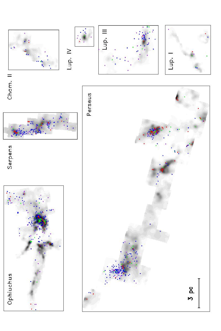


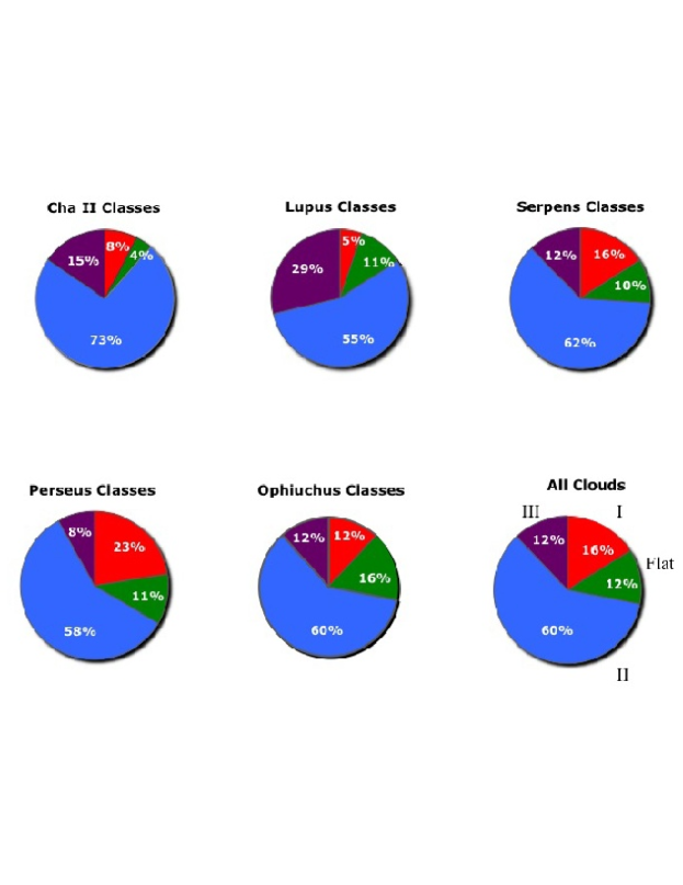

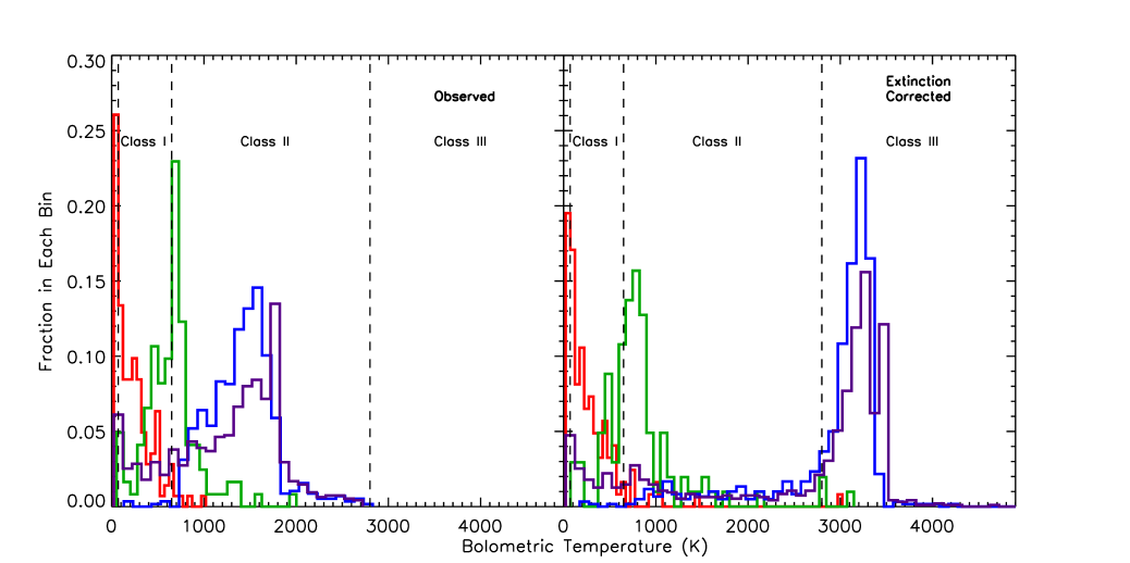
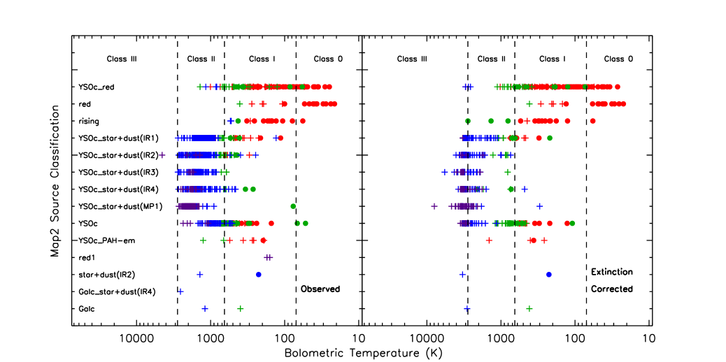

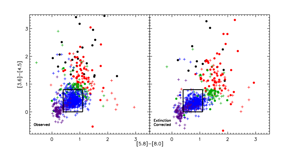
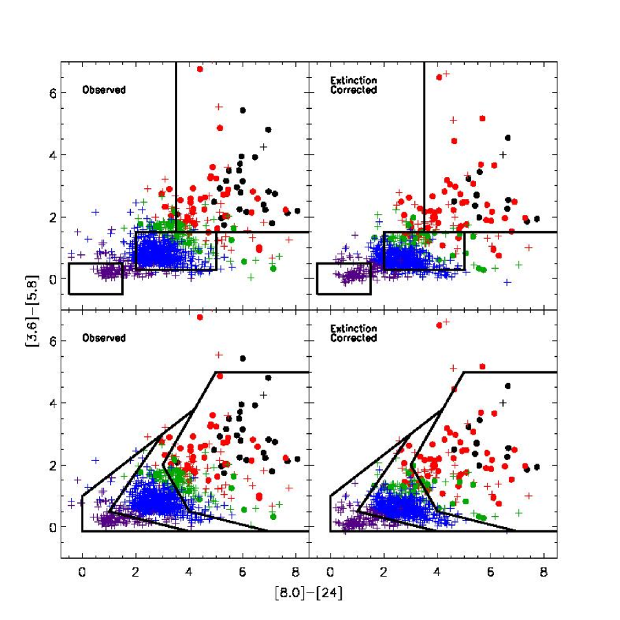
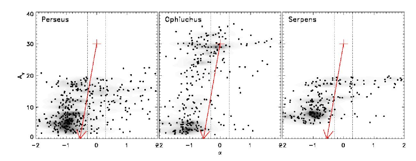
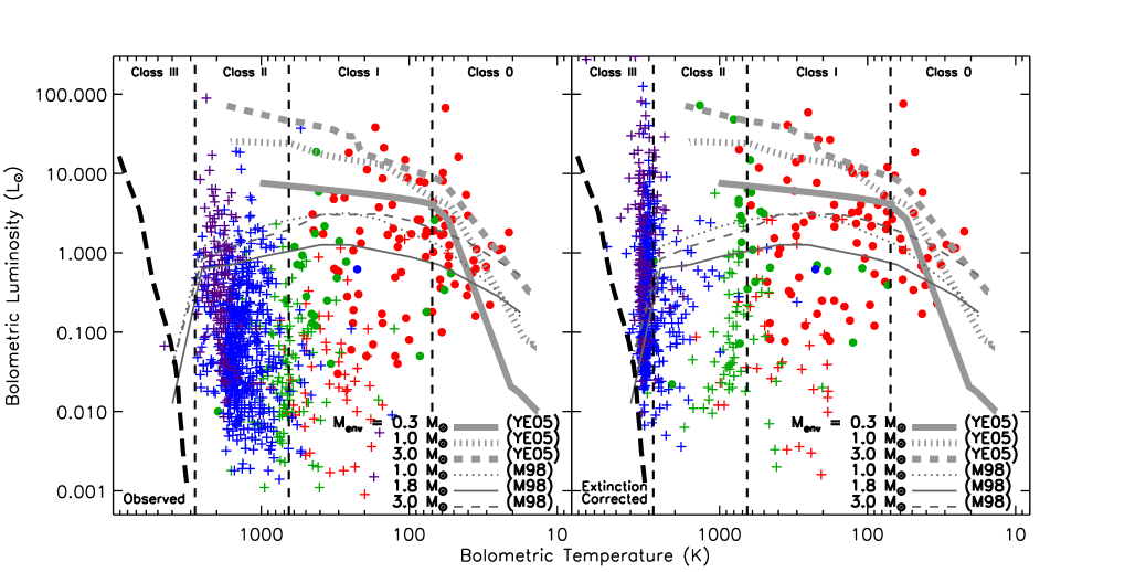

Appendix A Tables of YSOs
Table 8 contains the list of YSOs analyzed in this paper. The columns include a running index number, which is consistent throughout these tables, the JHK flux densities from 2MASS, flux densities from the four IRAC bands, and flux densities from the two shortest wavelength bands of MIPS. Additional flux densities from observations with other telescopes, at wavelengths ranging from 0.36 m to 1.3 mm, are presented in Tables 9, 10, and 11. The data are taken from Alcalá et al. (2008), Brede et al. (2008), Davis et al. (1999), Djupvik et al. (2006), Enoch et al. (2006), Enoch et al. (2007), Hatchell et al. (2005), Hatchell et al. (2007), Henning et al. (1993), Johnstone et al. (2000), Kirk et al. (2006), Merín et al. (2008a), Stanke et al. (2006), Tachihara et al. (2007), Wu et al. (2007), and Young et al. (2006).
Table 12 contains the derived properties for each source. The columns list, in order, the running index number, the name of the cloud containing the source, the official c2d source name, which includes the position information in J2000 coordinates, the c2d source classification, and the values for , , and , calculated from the observed flux densities. Following are the same three quantities (, , and ), calculated after correcting the flux densities for extinction, as described in §3.3. The next column indicates whether there is evidence for an envelope, as traced by extended millimeter continuum emission (e.g., Enoch et al. 2006, Young et al. 2006, Enoch et al. 2007). The last column has information on the reliability of the and values. “G” indicates existing photometry provides sufficient spectral coverage for reliable calculations; the uncertainties in both quantities are dominated by errors introduced by incomplete, finite sampling of the source SED and are typically % (Enoch et al. 2008a; Dunham et al. 2008). “L_I” indicates the source is associated with an envelope and thus likely an embedded source, but lacks spectral coverage between 24 m and 1 mm. The calculated values of and are thus considered lower and upper limits, respectively. “L_II” indicates the source is not associated with an envelope and has an observed 0.3, thus is not likely an embedded source, but no extinction correction could be derived based on available data, usually because of a lack of sufficient coverage in the near-infrared. The calculated values of and are thus considered lower limits.
The full tables are quite long and available only electronically. We provide samples of the tables in the print version.
| J | H | Ks | IRAC | IRAC | IRAC | IRAC | MIPS | MIPS | |
|---|---|---|---|---|---|---|---|---|---|
| Index | 1.25 m | 1.65 m | 2.17 m | 3.6 m | 4.5 m | 5.8 m | 5.8 m | 24 m | 70 m |
| 1 | 3100 29 | 5400 99 | 5900 54 | 2600 180 | 1500 92 | 1400 68 | 870 42 | 300 28 | 75 8.2 |
| 2 | 390 11 | 770 25 | 880 31 | 460 24 | 210 12 | 210 10 | 130 6.1 | 31 2.8 | … |
| 3 | 300 8.1 | 1600 75 | 5800 170 | … | … | 19000 3600 | 11000 3500 | … | 37000 3400 |
| 4 | 0.89 0.070 | 3.5 0.15 | 9.5 0.29 | 18 0.87 | 25 1.2 | 34 1.6 | 51 2.4 | 610 57 | 1500 150 |
| 5 | 51 1.5 | 78 2.4 | 86 2.5 | 73 4.0 | 67 3.3 | 61 2.9 | 57 2.7 | 51 4.7 | 40 5.7 |
| 6 | 12 0.35 | 1.0 0.29 | 8.7 0.25 | 5.9 0.29 | 4.9 0.24 | 3.9 0.20 | 3.1 0.15 | 0.82 0.21 | … |
| 7 | 160 4.4 | 270 7.5 | 300 8.2 | 290 15 | 250 13 | 260 13 | 330 16 | 380 36 | 170 19 |
| 8 | 1.5 0.060 | 4.2 0.12 | 6.3 0.21 | 7.1 0.35 | 6.8 0.34 | 6.7 0.33 | 7.0 0.33 | 8.1 0.76 | … |
| 9 | … | 2.7 0.12 | 38 1.1 | 210 10 | 440 26 | 640 31 | 700 34 | 3600 340 | 6200 600 |
| 10 | 1200 29 | 1800 55 | 1700 46 | 800 41 | 450 24 | 390 19 | 320 15 | 260 24 | … |
| U | B | V | R | H12 | I | m914 | z | |
|---|---|---|---|---|---|---|---|---|
| Index | 0.36 m | 0.44 m | 0.55 m | 0.64 m | 0.665 m | 0.79 m | 0.915 m | 0.96 m |
| 1 | … | 0.48 0.12 | 4.2 1.0 | 12 2.8 | 16 1.9 | 510 19 | … | … |
| 2 | … | 0.16 0.040 | 0.65 0.16 | 3.6 0.030 | 2.4 0.29 | 33 0.60 | 90 6.6 | 49 2.3 |
| 3 | … | 0.00100 0.0020 | 0.14 0.0040 | 0.83 0.00100 | 0.78 0.100 | 6.7 0.060 | 17 1.2 | 19 0.36 |
| 4 | … | … | … | 0.00100 0.00100 | 0.00100 0.00100 | 0.040 0.0020 | 0.090 0.00100 | 0.11 0.00100 |
| 5 | … | 0.40 0.00100 | 1.3 0.040 | 4.4 0.040 | 4.0 0.48 | 14 0.12 | 22 1.6 | 22 0.20 |
| 6 | 2.8 0.18 | 5.3 0.15 | 7.5 0.21 | 8.8 1.2 | 1.0 1.2 | 11 0.100 | 11 0.81 | 11 0.100 |
| 7 | … | 0.95 0.23 | 8.2 2.0 | 11 0.100 | 14 1.6 | 35 0.64 | 59 4.3 | 63 1.2 |
| 8 | … | … | … | 0.0030 0.00100 | … | 0.040 0.0020 | 0.18 0.020 | 0.18 0.00100 |
| 9 | … | … | … | … | … | … | … | … |
| 10 | … | 0.21 0.050 | … | 27 6.4 | 37 4.4 | 270 7.5 | … | … |
| L | M | ISO | IRAS | ISO | IRAS | IRAS | IRAS | |
|---|---|---|---|---|---|---|---|---|
| Index | 3.4 m | 5.0 m | 6.7 m | 12 m | 14.3 m | 25 m | 60 m | 100 m |
| 1 | 3500 32 | … | … | … | … | … | … | … |
| 2 | 540 5.0 | … | … | … | … | … | … | … |
| 3 | 12000 230 | 21000 590 | … | 44000 2200 | … | 100000 5100 | 110000 11000 | 100000 10000 |
| 4 | … | … | … | 110 20 | … | 900 180 | 3600 730 | 5100 1100 |
| 5 | 58 6.5 | … | … | … | … | 20 20 | … | … |
| 6 | 26 5.6 | … | … | … | … | … | … | … |
| 7 | 290 2.7 | … | … | 520 50 | … | 500 50 | 460 90 | 4300 1100 |
| 8 | … | … | 6.7 0.60 | … | 6.0 1.2 | … | … | … |
| 9 | … | … | 790 26 | 700 70 | 1200 25 | 4400 220 | 11000 530 | 18000 5400 |
| 10 | 840 7.7 | … | … | 380 40 | … | 360 30 | … | … |
| MIPS | |||||||
|---|---|---|---|---|---|---|---|
| Index | 160 m | 350 m | 450 m | 850 m | 1100 m | 1200 m | 1300 m |
| 1 | … | … | … | … | … | … | … |
| 2 | … | … | … | … | … | … | … |
| 3 | … | … | … | … | … | 1500 120 | 680 22 |
| 4 | 12000 2400 | … | … | … | … | … | 60 15 |
| 5 | … | … | … | … | … | … | … |
| 6 | … | … | … | … | … | … | … |
| 7 | … | … | … | … | … | … | … |
| 8 | … | … | … | … | … | … | … |
| 9 | 27000 2700 | … | … | … | … | 1900 130 | … |
| 10 | … | … | … | … | … | … | … |
| Spitzer | Observed | Extinction Corrected | ||||||||||
| Source Name | c2d | ′ | ′ | |||||||||
| Index | Cloud | (SSTc2d ) | Classification | AVaaThe Catalog values of are from the c2d catalog, based on a least-squares fit to any available data from 2 to 24 µm. IRAC values are based only on IRAC wavelengths. De-reddened values of or are based on extinction estimates from spectral types where available, assumption of a K7 spectral type otherwise for Class II and III sources. For Flat and Class 0/I sources, the mean extinction toward Class II sources in that cloud was assumed. The last two lines are based on Enoch et al. (2008a), who require a detection with Bolocam and thus refer only to the three clouds with such data. | (K) | (L⊙) | (K) | (L⊙) | EnvelopebbIndicates whether or not the source is associated with an envelope as traced by extended millimeter emission (based primarily on the sample of Enoch et al. [2008]). | QualityccIndicates the quality of the calculated and values.
“G”: existing photometry provides sufficient spectral coverage for reliable calculations. Other flags mark sources without sufficient coverage: “L_I”: the source is associated with an envelope and thus likely an embedded source, but lacks spectral coverage between 24 m and 1 mm. The calculated values of and are thus considered lower and upper limits, respectively. “L_II”: the source is not associated with an envelope and has an observed 0.3, thus is not likely an embedded source, but no extinction correction could be derived based on available data, usually because of a lack of sufficient coverage in the near-infrared. The calculated values of and are thus considered lower limits. “O”: Other. These three sources were added to the list of YSOs based on the searches for embedded protostars presented by Jørgensen et al. (2007) (for Perseus) and Jørgensen et al. (2008) (for Ophiuchus), but they are not associated with envelopes according to Enoch et al. (2008). They are only detected at one wavelength (24 m), thus calculations of , , and are not possible. They are counted as Class I objects when classifying by and ; they are not counted at all when classifying by and ′. |
||
| 1 | Cham II | J124825.74770636.5 | YSOc_stardust(MP1) | 4.4 | 2.19 | 2200 | 11 | 2.59 | 3000 | 28 | N | G |
| 2 | Cham II | J125230.66771513.0 | YSOc_stardust(MP1) | 4.3 | 2.38 | 2100 | 1.4 | 2.71 | 2700 | 3.2 | N | G |
| 3 | Cham II | J125317.23770710.7 | rising | 10.5 | 0.72 | 550 | 38 | 0.14 | 1400 | 72 | N | G |
| 4 | Cham II | J125342.86771511.5 | YSOc_red | 4.0 | 0.65 | 120 | 0.49 | 0.21 | 190 | 0.59 | Y | G |
| 5 | Cham II | J125633.66764545.3 | YSOc_stardust(IR2) | 2.4 | 1.22 | 2200 | 0.21 | 1.35 | 2900 | 0.36 | N | G |
| 6 | Cham II | J125658.68764706.6 | YSOc_stardust(IR2) | 0.0 | 1.84 | 4500 | 0.067 | 1.84 | 4500 | 0.067 | N | L_II |
| 7 | Cham II | J125711.77764011.3 | YSOc_stardust(IR1) | 3.3 | 0.85 | 1800 | 0.86 | 1.06 | 3100 | 1.8 | N | G |
| 8 | Cham II | J125806.78770909.4 | YSOc_stardust(IR1) | 5.0 | 0.93 | 1400 | 0.013 | 1.09 | 1900 | 0.020 | N | G |
| 9 | Cham II | J125906.58770739.9 | YSOc_red | 4.0 | 0.68 | 220 | 1.9 | 0.49 | 270 | 2.4 | Y | G |
| 10 | Cham II | J125926.45774708.4 | YSOc_stardust(IR4) | 3.9 | 1.78 | 2400 | 3.7 | 2.01 | 3300 | 9.8 | N | G |