Parts and Wholes

An Inquiry into
Quantum and Classical Correlations

M.P. Seevinck

Note on the different arXiv versions:

 This version arXiv/0811.1027v3 (24 April 2009) has exactly the same content as the version arXiv/0811.1027v2 (7 November 2008). However, the page layout has been changed so that it is the same as the distributed hard copy version of the Dissertation which is on B5 format.

Colofon

Financial support by the Institute for History and Philosophy of Science, Utrecht University.

Copyright © 2008 by Michael Patrick Seevinck. All rights reserved.

Cover design by Ivo van Sluis.
Printed in the Netherlands by PrintPartners Ipskamp, Enschede.
Printed on FSC certified paper.

ISBN 978-90-3934916-8

Promotor:  Prof.dr. D.G.B.J. Dieks

Co-promotor: Dr. J.B.M. Uffink

  

Now it is precisely in cleaning up intuitive ideas for mathematics that one is likely to throw out the baby with the bathwater.

           J.S. Bell ; ‘La nouvelle cuisine’, 1990.

Preface

Not to be found in this dissertation is a love story – the story of the genesis of this dissertation. Just like any love story it cannot but be a tragic one. Full of happiness and despair, joy and sorrow. I believe a few words about this story are in order here.

The story began with love at first sight, but it took many years for this to become a true love and develop into a somewhat steady relationship. This rather slow start is due to the circumstance that when I started with the current project I was rehabilitating from a previous similar love affair, and this made me hesitant and rather uncertain of how to proceed. But luckily, things changed. The great intellectual freedom I granted myself, and which was also made possible by the carte blanche handed to me at the beginning of the project, provided ideal circumstances for falling in love, and thus for rediscovering the truth-lover inside of me. The present dissertation stems from that love of truth – but this occurred not without difficulty, be it mentioned.

The intellectual freedom may further explain the fact that this dissertation is not concerned with a single research question, but with a handful of different, though related subjects, and also that my love produced many ideas, only some of which turned out to be promising, whereas many were in fact utter nonsense. The latter is not to be regretted for I am convinced that a love of truth can only really be creative when it does not fear misfortune, nor mistake or confusion.

I invite the reader to try and taste some of the fruits of this love. I believe – and sincerely hope – that some may taste delicious, but I realize that others may very well be rather bland and tasteless.

With these final words an episode has come to an end. Fortunately, the story continues — forever learning how to truly love.

M.P. Seevinck

Nijmegen, September 2008

Chapter 2 On correlations:
Definitions and general framework

This chapter is in part based on seevchen.

2.1 Introduction

In this chapter we give the necessary background for discussing the technical results of this dissertation. We will present the definitions, notation and techniques that will be used in later chapters, as well as several clarifying examples. We also discuss relevant results already obtained by others. Along the way we will take the opportunity to indicate more precisely than was done in the previous chapter what technical results are contained in later chapters. The foundational relevance of the results will be discussed later. For conciseness and clarity of exposition we will for now refrain from any interpretational discussion.

We start in section 2.2 by defining the different kinds of correlation that will be studied, as well as several useful mathematical characteristics of these correlations. We follow the approach by barrett05 and masanes06 in discussing the no-signaling, local and quantum correlations, and we will supplement their presentation with a new type of correlations, the partially-local correlations. Discerning these different kinds of correlations is in general a hard task. In section 2.3 we will argue that Bell-type inequalities form a useful tool for this task. We present a general scheme for describing such inequalities in terms of bounds on the expectation values of so-called Bell-type polynomials. After discussing this scheme we present the well-known bi-partite Clauser-Horne-Shimony-Holt (CHSH) inequality chsh as an example. This inequality discriminates some of the bi-partite correlations, but, as we will show, not all of them. We will then further comment on the task of obtaining multi-partite Bell-type inequalities in order to discriminate the different types of multipartite correlations.

We next pay special attention to the issue of discriminating quantum correlations, because here the distinction between entanglement and separability of quantum states becomes relevant. In the bi-partite case we discuss the feature of separability and entanglement, and the (non-)locality of these states.

Lastly, in section 2.4 we discuss a possible pitfall connected to the use of Bell-type polynomials for obtaining Bell-type inequalities. We trace the problem back to the fact that Bell-type inequalities always use different combinations of incompatible observables. This re-teaches an old lesson from J.S. Bell, namely, that one should be extremely careful when considering incompatible observables, and not be lured into neglecting this issue because quantum mechanics deals so easily with incompatible observables via the non-commutativity structure that is part and parcel of its formalism.

2.2 Correlations

2.2.1 General correlations

Consider $N$ parties, labeled by $1,2,\ldots,N$, each holding a physical system that are to be measured using a finite set of different observables. Denote by $A_{j}$ the observable (random variable) that party $j$ chooses (also called the setting $A_{j}$) and by $a_{j}$ the corresponding measurement outcomes. We assume there to be only a finite number of discrete outcomes. The outcomes can be correlated in an arbitrary way. A general way of describing this situation, independent of the underlying physical model, is by a set of joint probability distributions for the outcomes, conditioned on the settings chosen by the $N$ parties, where the correlations are captured in terms of these joint probability distributions. They are denoted by

$$P(a_{1},\ldots,a_{N}|A_{1},\ldots,A_{N}).$$ (2.1)

These probability distributions are assumed to be positive

$$P(a_{1},\ldots,a_{N}|A_{1},\ldots,A_{N})\geq 0,\leavevmode\nobreak\ \leavevmode\nobreak\ \forall a_{1},\ldots,a_{N},\leavevmode\nobreak\ \leavevmode\nobreak\ \forall A_{1},\ldots,A_{N},$$ (2.2)

and obey the normalization conditions

$$\sum_{a_{1},\ldots,a_{N}}P(a_{1},\ldots,a_{N}|A_{1},\ldots,A_{N})=1,\leavevmode\nobreak\ \leavevmode\nobreak\ \forall A_{1},\ldots,A_{N}.$$ (2.3)

We need not demand that the probabilities should not be greater than 1 because this follows from them being positive and from the normalization conditions.

The set of all these probability distributions has a nice structure. First, it is a convex set: convex combinations of correlations are still legitimate correlations. Second, there are only a finite number of extremal correlations. This means that every correlation can be decomposed into a (not necessarily unique) convex combination of such extremal correlations.

A total of $D=\prod_{i=1}^{N}m_{A_{i}}m_{a_{i}}$ different probabilities exist (here $m_{A_{i}}$ and $m_{a_{i}}$ are the number of different observables and outcomes for party $i$ respectively). When these conditional probability distributions (2.1) are considered as points in a $D$-dimensional real space, this set of points forms a convex polytope with a finite number of extreme points which are the vertices of the polytope. This polytope is the convex hull of the extreme points. It belongs to the subspace defined by (2.3) and it is bounded by a set of facets, linear inequalities that describe the halfplanes that bound it. Every convex polytope has a dual description, firstly in terms of its vertices, and secondly in terms of its facets, i.e., hyperplanes that bound the polytope uniquely. In general each facet can be described by linear combinations of joint probabilities which reach a maximum value at the facet, i.e.,

$$\sum_{a_{1},\ldots,a_{N},A_{1},\ldots,A_{N}}c_{a_{1},\ldots,a_{N},A_{1},\ldots,A_{N}}P(a_{1},\ldots,a_{N}|A_{1},\ldots,A_{N})\leq I,$$ (2.4)

with real coefficients $c_{a_{1},\ldots,a_{N},A_{1},\ldots,A_{N}}$ and a real bound $I$ that is reached by some extreme points. For each facet some extreme points of the polytope lie on this facet and thus saturate the inequality (2.4), while the other extreme points cannot violate it. In general, when the extreme points are considered as vectors, a hyperplane is a facet of a $d$-dimensional polytope iff $d$ affinely independent extreme points satisfy the equality that characterizes the hyperplane. Consequently, for the case of general correlations (2.1) the set of extreme points that lie on a facet must contain a total of $D$ affinely independent vectors. For this case the facets are determined by equality in (2.2). The probability distributions (2.1) correspond to any normalized vector of positive numbers in this polytope. For an excellent overview of the structure of these polytopes, see masanes02, barrett05 and ziegler.

The extreme points are the probability distributions that saturate a maximum of the positivity conditions (2.2) while satisfying the normalization condition (2.3). They are characterized by jones to be the probability distributions such that for each set of settings $\{A_{1},\ldots,A_{N}\}$ there is a unique set of outcomes $\{a_{1}[A_{1},\ldots A_{N}],\ldots,a_{N}[A_{1},\ldots A_{N}]\}$ for which $P(a_{1},\ldots,a_{N}|A_{1},\ldots,A_{N})=1$, with $a_{1}[A_{1},\ldots,A_{N}]$ the deterministic determination of outcome $a_{1}$ given the settings $A_{1},\ldots,A_{N}$, etc. There is thus a one-to-one correspondence between the extreme points and the sets of functions $\{a_{1}[A_{1},\ldots A_{N}],\ldots,a_{N}[A_{1},\ldots A_{N}]\}$ from the settings to the outcomes. Any such set defines an extreme point. The extreme points thus correspond to deterministic scenarios: each outcome is completely fixed by the totality of all settings and consequently there is no randomness left: $P(a_{1},\ldots,a_{N}|A_{1},\ldots,A_{N})=\delta_{a_{1},a_{1}[A_{1},\ldots,A_{N}]}\cdots\delta_{a_{N},a_{N}[A_{1},\ldots,A_{N}]}$. Finding all the facets of a polytope knowing its vertices is called the hull problem and this is in general a computationally hard task pitowsky. The facet descriptions (2.4) will be called Bell-type inequalities, and these will be further introduced later.

The marginal probabilities are obtained in the usual way from the joint probabilities by summing over the outcomes of the other parties. It is important to realize that for general correlations these marginals may depend on the settings chosen by the other parties. For example, in the case of two parties that each choose two possible settings $A_{1},A_{1}^{\prime}$ and $A_{2},A_{2}^{\prime}$ respectively, the marginals for party 1 are given by

$$P(a_{1}|A_{1})^{A_{2}} :=\sum_{a_{2}}P(a_{1},a_{2}|A_{1},A_{2}),$$ (2.5a)

$$P(a_{1}|A_{1})^{A_{2}^{\prime}} :=\sum_{a_{2}}P(a_{1},a_{2}|A_{1},A_{2}^{\prime}),$$ (2.5b)

and analogously for setting $A_{1}^{\prime}$ and for the marginals of party 2. The marginal $P(a_{1}|A_{1})^{A_{2}}$ may thus in general be different from $P(a_{1}|A_{1})^{A_{2}^{\prime}}$.

We will now put further restrictions besides normalization on the probability distributions (2.1) that are motivated by physical considerations. We will here not be concerned with arguing for the plausibility of these physical considerations, nor what violations of these physically motivated restrictions amounts to, but merely give the definitions that will be used in future chapters. There we will comment on the foundational content of the restrictions and their possible violations.

2.2.2 No-signaling correlations

Let us first consider the case of two parties that each choose two possible settings. A no-signaling correlation for two parties is a correlation such that party $1$ cannot signal to party $2$ by the choice of what observable is measured by party $1$ and vice versa. This means that the marginal probabilities $P(a_{1}|A_{1})^{A_{2}}$ (see (2.5a)) and $P(a_{2}|A_{2})^{A_{1}}$ are independent of $A_{2}$ and $A_{1}$ respectively:

$$P(a_{1}|A_{1})^{A_{2}}=P(a_{1}|A_{1})^{A_{2}^{\prime}} :=P(a_{1}|A_{1}),\leavevmode\nobreak\ \leavevmode\nobreak\ \forall a_{1},A_{1},A_{2},A_{2}^{\prime},$$ (2.6a)

$$P(a_{2}|A_{2})^{A_{1}}=P(a_{2}|A_{2})^{A_{1}^{\prime}} :=P(a_{2}|A_{2}),\leavevmode\nobreak\ \leavevmode\nobreak\ \forall a_{2},A_{1},A_{1}^{\prime},A_{2}.$$ (2.6b)

In a no-signaling context the marginals can thus be defined as $P(a_{1}|A_{1})$, etc., i.e., without any dependence on far-away settings.

Let us generalize this to the multi-partite setting: a no-signaling correlation is a correlation $P(a_{1},\ldots,a_{N}|A_{1},\ldots,A_{N})$ such that one subset of parties, say parties $1,2,\ldots,k$, cannot signal to the other parties $k-1,\ldots,N$ by changing their measurement device settings $A_{1},\ldots,A_{k}$. Mathematically this is expressed as follows. The marginal probability distribution for each subset of parties only depends on the corresponding observables measured by the parties in the subset, i.e., for all outcomes $a_{k+1},\ldots,a_{N}$: $P(a_{1},\ldots,a_{k}|A_{1},\ldots,A_{N})=P(a_{1},\ldots,a_{k}|A_{1},\ldots,A_{k})$. These conditions can all be derived from the following condition barrett05. For each $k\in\{1,\ldots,N\}$ the marginal distribution that is obtained when tracing out $a_{k}$ is independent of what observable ($A_{k}$ or $A_{k}^{\prime}$) is measured by party $k$:

$$\sum_{a_{k}}P(a_{1},\ldots,a_{k},\ldots,a_{N}| A_{1},\ldots,A_{k},\ldots,A_{N})=$$

$$\sum_{a_{k}}P(a_{1},\ldots,a_{k},\ldots,a_{N}|A_{1},\ldots,A_{k}^{\prime},\ldots,A_{N}),$$ (2.7)

for all outcomes $a_{1},\ldots,a_{k-1},a_{k+1},\ldots,a_{N}$ and all settings $A_{1},\ldots,A_{k},A_{k}^{\prime},\ldots A_{N}$. This set of conditions ensures that all marginal probabilities are independent of the settings corresponding to the outcomes that are no longer considered. In particular, (2.2.2) the defines the marginal

$$P(a_{1},\ldots,a_{k-1},a_{k+1},\ldots,a_{N}|A_{1},\ldots,A_{k-1},A_{k+1},\ldots,A_{N}),$$ (2.10)

for the $N-1$ parties not including party $k$. No-signaling ensures that it is not needed to specify whether $A_{k}$ or $A_{k}^{\prime}$ is being measured by party $k$.

These linear equations (2.2.2) characterize an affine set masanes06. The intersection of this set with the polytope of distributions (2.1) gives another convex polytope: the no-signaling polytope. The vertices of this polytope can be split into two types: vertices that correspond to deterministic scenarios, where all probabilities are either $0$ or $1$, and those that correspond to non-deterministic scenarios. All no-signaling deterministic correlations are in fact local masanes06, i.e., they can be written in terms of the local correlations defined below on page 2.2.3. But all non-deterministic vertices correspond to non-local scenarios.

The complete set of vertices of the no-signaling polytope is in general unknown. However, in the bi-partite and three-partite case some results have been obtained: For the bi-partite case of two settings and any number of outcomes they are determined by barrett05 and for any number of settings and two possible outcomes by jonesmasanes. For three parties, two outcomes and two settings the vertices are given in barrett05.

The facets of the no-signaling polytope follow from the defining conditions for no-signaling correlations. These are thus the trivial facets that follow from the positivity conditions as well as the non-trivial ones that follow from the no-signaling requirements (2.2.2). In section 2.3.1.1 the latter will be explicitly dealt with in the two-partite case. The importance of the non-trivial facets of the no-signaling polytope is that if a point, representing some experimental data, lies within the polytope, then a model that uses no-signaling correlations exists that reproduces the same data. On the contrary, if the point lies outside the polytope and thus violates some Bell-type inequality describing a facet of the no-signaling polytope, then the data cannot be reproduced by a no-signaling model only, i.e., including some signaling is necessary.

2.2.3 Local correlations

Local correlations are those that can be obtained if the parties are non-communica-ting and share classical information, i.e., they only have local operations and local hidden variables (also called shared randomness) as a resource. We take this to mean that these correlations can be written as

$$P(a_{1},\ldots,a_{N}|A_{1},\ldots,A_{N})=\int_{\Lambda}d\lambda p(\lambda)P(a_{1}|A_{1},\lambda)\ldots P(a_{N}|A_{N},\lambda),$$ (2.11)

where $\lambda\in\Lambda$ is the value of the shared local hidden variable, $\Lambda$ the space of all hidden variables and $p(\lambda)$ is the probability that a particular value of $\lambda$ occurs. Note that $p(\lambda)$ is independent of the outcomes $a_{j}$ and settings $A_{j}$. This is a ‘freedom’ assumption, i.e., the settings are assumed to be free variables (we will discuss this assumption in the next chapter). Furthermore, $P(a_{1}|A_{1},\lambda)$ is the probability that outcome $a_{1}$ is obtained by party $1$ given that the observable measured was $A_{1}$ and the shared hidden variable was $\lambda$, and similarly for the other terms $P(a_{k}|A_{k},\lambda)$. Since these probabilities are conditioned on the hidden variable $\lambda$ we will call them subsurface probabilities, in contradistinction to the probabilities $P(a_{j}|A_{j})$, etc., that only conditionalize on the settings, which we call surface probabilities.

Condition (2.11) is supposed to capture the idea of locality in a hidden-variable framework and it is called Factorisability, and models that give only local correlations are called local hidden-variable (LHV) models. These notions will be further discussed in the next chapter. Correlations that cannot be written as (2.11) are called non-local. Local correlations are no-signaling thus the marginal probabilities derived from local correlations are defined in the same way as was done for no-signaling correlations, cf. (2.10).

Let us review what is known about the set of local correlations. First, it is also a polytope with vertices (extremal points) corresponding to local deterministic distributions werwolf, i.e., $P(a_{1},\ldots,a_{N}|A_{1},\ldots,A_{N})=\delta_{a_{1},a_{1}[A_{1}]}\cdots\delta_{a_{N},a_{N}[A_{N}]}$ where the function $a_{1}[A_{1}]$ gives the deterministic determination of outcome $a_{1}$ given the setting $A_{1}$, etc. Thus for each set of settings $\{A_{1},\ldots,A_{N}\}$ there is a unique set of outcomes $\{a_{1}[A_{1}],\ldots,a_{N}[A_{N}]\}$ for which $P(a_{1},\ldots,a_{N}|A_{1},\ldots,A_{N})=1$. All these vertices are also vertices of the no-signaling polytope barrett05. The local polytope is known to be constrained by two kinds of facets werwolf. The first are trivial facets and derive from the positivity conditions (2.2). Note that these are also trivial facets of the no-signaling polytope. The second kind of facets are non-trivial and can be violated by non-local correlations. These are not facets of the no-signaling polytope. All facets are mathematically described by Bell-type inequalities (2.4), that will be further introduced below. Determining whether a point lies within the local polytope, i.e., whether it does not violate a local Bell-type inequality, is in general very hard as pitowsky has shown this to be related to some known hard problems in computational complexity (i.e., it is an NP-complete problem). Furthermore, determining whether a given inequality is a facet of the local polytope is of similar difficulty (i.e., this problem is co-NP complete pitowsky91).

2.2.4 Partially-local correlations

Partially local correlations are those that can be obtained from an $N$-partite system in which subsets of the $N$ parties form extended systems, whose internal states can be correlated in any way (e.g., signaling), which however behave local with respect to each other. Suppose provisionally that parties $1,\ldots,k$ form such a subset and the remaining parties $k+1,\ldots,N$ form another subset. The partially-local correlations can then be written as

$$P(a_{1},\ldots, \,a_{N}|A_{1},\ldots,A_{N})=$$ (2.12)

$$\int_{\Lambda}d\lambda p(\lambda)P(a_{1},\ldots,a_{k}|A_{1},\ldots,A_{k},\lambda)P(a_{N-k},\ldots,a_{N}|A_{N-k},\ldots,A_{N},\lambda),$$

We also refer to this condition as partial factorisability. The subsurface probabilities on the right hand side need not factorise any further. In case they would all fully factorise we retrieve the set of local correlations described above.

Formulas similar to (2.12) with different partitions of the $N$-parties into two subsets, i.e., for different choices of the composing parties and different values of $k$, describe other possibilities to give partially-local correlations. Convex combinations of these possibilities are also admissible. We need not consider decomposition into more than two subsystems since any two subsystems in such a decomposition can be considered jointly as parts of one subsystem still uncorrelated with respect to the others.

We define a model to have partially-local correlations when the correlations are of the form (2.12) or when they can be written as convex combinations of similar expressions on the right hand side of (2.12) for the different possible partitions of the $N$ parties into two subsets. Such a model is called a partially-local hidden-variable (PHLV) model. Models whose correlations cannot be written in this partially-local form are fully non-local, i.e., they are said to contain full non-locality.

The set of partially-local correlations has a finite number of extreme points and is thus also a polytope jones, called the partially-local polytope. It is also convex since it can be easily seen that if two distributions satisfy (2.12) then their convex mixture will too. For each extreme point of this convex polytope there is a partition into two subsets, say $\{1,\ldots,k\}$ and $\{k+1,\ldots,N\}$, such that for each set of settings $\{A_{1},\ldots,A_{N}\}$ there is a unique set of outcomes $\{a_{1}\ldots,a_{N}\}$ for which $P(a_{1},\ldots,a_{k}|A_{1},\ldots,A_{k},\lambda)=1$ and $P(a_{N-k},\ldots,a_{N}|A_{N-k},\ldots,A_{N},\lambda)=1$. There is thus a one-to-one correspondence between the extreme points corresponding to a partition of the parties into two subsets and the set of functions from the two corresponding subsets of settings to the two corresponding subsets of outcomes. Just as was the case for general and local correlations, we again see the deterministic scenario arising for the extreme points.

Let us consider this in more detail and take the example where $N=3$, first studied by svetlichny. Only three different partitions into two subsets are possible. The three-partite partially-local correlations are thus of the form

$$P(a_{1},a_{2},a_{3}|A_{1},A_{2},A_{3})=\int_{\Lambda}d\lambda[ p_{1}\,\rho_{1}(\lambda)P_{1}(a_{1}|A_{1},\lambda)P_{1}(a_{2},a_{3}|A_{2},A_{3},\lambda)$$

$$+p_{2}\,\rho_{2}(\lambda)P_{2}(a_{2}|A_{2},\lambda)P_{2}(a_{1},a_{3}|A_{1},A_{3},\lambda)$$

$$+p_{3}\,\rho_{3}(\lambda)P_{3}(a_{3}|A_{3},\lambda)P_{3}(a_{1},a_{2}|A_{1},A_{2},\lambda)].$$ (2.13)

where $P_{1}(a_{2},a_{3}|A_{2},A_{3},\lambda)$ can be any probability distribution; it need not factorise into $P_{1}(a_{2}|A_{2},\lambda)P_{1}(a_{3}|A_{3},\lambda)$. Analogously for the other two joint probability terms. The $\rho_{i}(\lambda)$ are the hidden-variable distributions. Models whose correlations cannot be written in this form are fully non-local, i.e., they are said to contain full three-partite non-locality.

Because the correlations between subsets of particles are allowed to be signaling, the marginal probabilities may depend on the settings corresponding to the outcomes that are no longer considered. This must be explicitly accounted for. For example, the marginal $P(a_{1},a_{2},|A_{1},A_{2})^{A_{3}}$ derived from (2.13) may depend on the setting chosen by party $3$, and the marginal $P(a_{1}|A_{1})^{A_{2},A_{3}}$ for party $1$ may depend on the setting chosen by both party 2 and 3, etc. Because we must allow for convex combinations of different partially-local configurations, as in (2.13), the marginals can depend on the settings chosen by all other parties, despite the fact that at the hidden variable level there can not be signaling between all three parties.

2.2.5 Quantum correlations

Lastly, we consider another class of correlations: those that are obtained by general measurements on quantum states (i.e., those that can be generated if the parties share quantum states). These can be written as

$$P(a_{1},\ldots,a_{N}|A_{1},\ldots,A_{N})=\textrm{Tr}[M_{a_{1}}^{A_{1}}\otimes\cdots\otimes M_{a_{N}}^{A_{N}}\rho].$$ (2.14)

Here $\rho$ is a quantum state (i.e., a unit trace semi-definite positive operator) on a Hilbert space $\mathcal{H}=\mathcal{H}_{1}\otimes\cdots\otimes\mathcal{H}_{N}$, where $\mathcal{H}_{j}$ is the quantum state space of the system held by party $j$. The sets $\{M_{a_{1}}^{A_{1}},\ldots,M_{a_{N}}^{A_{N}}\}$ define what is called a positive operator valued measure (POVM), i.e., a set of positive operators $\{M_{a_{j}}^{A_{j}}\}$ satisfying $\sum_{a_{j}}M_{a_{j}}^{A_{j}}=\mathds{1},\forall A_{j}$. Of course, all operators $M_{a_{j}}^{A_{j}}$ must commute for different $j$ in order for the joint probability distribution to be well defined, but this is ensured since for different $j$ the operators are defined for different subsystems (with each their own Hilbert space) and are therefore commuting. Note that (2.14) is linear in both $M_{a_{j}}^{A_{j}}$ and $\rho$, which is a crucial feature of quantum mechanics.

Quantum correlations are no-signaling and therefore the marginal probabilities derived from such correlations are defined in the same way as was done for no-signaling correlations (cf. (2.10)). For example, the marginal probability for party $1$ is given by $P(a_{1}|A_{1})=\textrm{Tr}[M_{a_{1}}^{A_{1}}\rho^{1}]$, where $\rho^{1}$ is the reduced state for party 1.

The set of quantum correlations has been investigated by, e.g., pitowsky, tsirelsonhodronic, and wernerwolf2 and is shown to be convex. It is not a polytope because the number of extremal points is not finite and consequently it has an infinite number of bounding halfplanes. Therefore we will refer to this set as the quantum body, in contradistinction to the sets of the other types of correlations which are referred to as polytopes.

We note that in order to describe the full measurement process it is necessary to specify the set of so-called Kraus operators $\{K_{a_{i}}^{A_{i}}\}$ that correspond to the POVM elements $\{M_{a_{i}}^{A_{i}}\}$, where $M_{a_{i}}^{A_{i}}=K_{a_{i}}^{A_{i}}(K_{a_{i}}^{A_{i}})^{\dagger}$. In general many different sets of Kraus operators correspond to the same POVM element. The reason for including the Kraus operators is that the description of a POVM as a set of positive operators $\{M_{a_{i}}^{A_{i}}\}$ is incomplete because it does not specify uniquely what the state of the system is after the measurement. By including the Kraus operators one is able to retrieve the Projection Postulate: if a POVM measurement is performed on system $i$ then the state $\rho_{i}$ directly after the measurement will be given by $\tilde{\rho}_{i}=K_{a_{i}}^{A_{i}}\,\rho_{i}\,(K_{a_{i}}^{A_{i}})^{\dagger}\,/\,{\rm Tr}[K_{a_{i}}^{A_{i}}\,\rho_{i}\,(K_{a_{i}}^{A_{i}})^{\dagger}]$.

2.3 On comparing and discriminating the different kinds of correlations

Let us present the relationships between the correlations of the previous section, some of which are already known, some of which are proven in this dissertation. The polytope of general correlations strictly contains the no-signaling polytope, which in turn contains the quantum body, which in turn contains the partially-local polytope, which in turn contains the local polytope. See Figure 2.1. These results are obtained by comparing the facets of the relevant polytopes and halfplanes that bound the quantum bodies. These facets (i.e., bounding hyperplanes in the case of quantum correlations) are of course implicitly determined by the defining restrictions on the different types of correlations, but to find explicit experimentally accessible expressions for them is a hard job. A fruitful way of doing so is using so-called Bell-type inequalities. This will be discussed next.

Figure 2.1: Schematic representation of the space of correlations, after barrett05. The vertices are labeled L, PL and NL for the local, partially-local and no-signaling polytope. The region inside each of these polytopes is denoted by $\mathcal{L}$, $\mathcal{P}$, and $\mathcal{N}$ respectively. The accessible quantum region is denoted by $\mathcal{Q}$.

2.3.1 Bell-type inequalities: finding experimentally
accessible bounds that discriminate between
different types of correlations

In this dissertation we will investigate all of the above types of correlations by deriving experimentally accessible conditions that distinguish them from one another. In particular we will study Bell-type inequalities for the case where each party chooses between two alternative observables and where each observable is dichotomic, i.e., the observable has two possible outcomes which we denote by $\pm 1$.

Bell-type inequalities denote a specific bound on a linear sum of joint probabilities as in (2.4). The bound is characteristic of the type of correlation under study. However, frequently they are formulated not in terms of probabilities but in terms of product expectation values, i.e., expectation values of products of observables, which we will denote by $\langle A_{1}A_{2}\cdots A_{N}\rangle$. These are defined in the usual way as the weighted sum of the products of the outcomes:

$$\langle A_{1}A_{2}\cdots A_{N}\rangle:=\sum_{a_{1},\ldots,a_{N}}a_{1}a_{2}\cdots a_{N}P(a_{1},\ldots,a_{N}|A_{1},\ldots,A_{N}).$$ (2.15)

Since we are restricting ourselves to dichotomic observables with outcomes $\pm 1$ all expectation values are bounded by: $-1\leq\langle A_{1}A_{2}\cdots A_{N}\rangle\leq 1$, for all $A_{1},A_{2},\ldots,A_{N}$.

The probabilities $P(a_{1},\ldots,a_{N}|A_{1},\ldots,A_{N})$ in (2.15) are determined using the different kinds of correlations we have previously defined. If they are of the local form (2.11) we denote the product expectation values they give rise to by $\langle A_{1}A_{2}\cdots A_{N}\rangle_{\textrm{lhv}}$, and analogously for other types of correlation. This is captured in table 2.1.

type notation $P(a_{1},\ldots,a_{N}|A_{1},\ldots,A_{N})$ in (2.15) given by no-signaling $\langle A_{1}A_{2}\cdots A_{N}\rangle_{\textrm{ns}}$ (2.2.2) local $\langle A_{1}A_{2}\cdots A_{N}\rangle_{\textrm{lhv}}$ (2.11) partially-local $\langle A_{1}A_{2}\cdots A_{N}\rangle_{\textrm{plhv}}$ (2.12) quantum $\langle A_{1}A_{2}\cdots A_{N}\rangle_{\textrm{qm}}$ (2.14)

Table 2.1: The different kinds of product expectation values that arise from the different kinds of correlations.

We will investigate the different possible correlations using Bell-type inequalities in terms of product expectation values as given in table 2.1. We will not investigate them directly in terms of the joint probabilities. The main reason for this is that using the product expectation values simplifies the investigation considerably. For example, consider the case of two parties that each measure two dichotomous observables each. We denoted them as $A_{1},A_{1}^{\prime}$ and $A_{2},A_{2}^{\prime}$ respectively, with outcomes $a_{1},a_{1}^{\prime}$ and $a_{2},a_{2}^{\prime}$. Instead of dealing with the $16$-dimensional space of vectors with components $P(a_{1},a_{2}|A_{1},A_{2}),P(a_{1}^{\prime},a_{2}|A_{1},A_{2}),\ldots,P(a_{1}^{\prime},a_{2}^{\prime}|A_{1}^{\prime},A_{2}^{\prime})$ we only have to deal with the $4$-dimensional vectors that have as components the quantities $\langle A_{1},A_{2}\rangle$,$\langle A_{1},A_{2}^{\prime}\rangle$,$\langle A_{1}^{\prime},A_{2}\rangle$,$\langle A_{1}^{\prime},A_{2}^{\prime}\rangle$. To transform a vector from the $16$-dimensional space to its corresponding $4$-dimensional space, one needs to perform a projection as given in (2.15). It is known that the projection of a convex polytope is always a convex polytope masanes02. Therefore, the convex polytopes we have considered previously for general, no-signaling, partially-local and local correlations in the higher dimensional joint probability space correspond to convex polytopes in the lower dimensional space of product expectation values. The set of vectors with components $\langle A_{1},A_{2}\rangle,\langle A_{1},A_{2}^{\prime}\rangle,\langle A_{1}^{\prime},A_{2}\rangle,\langle A_{1}^{\prime},A_{2}^{\prime}\rangle$ that are attainable by general, no-signaling, partially-local and local correlations are thus also characterized by a finite set of extreme points and corresponding facets.

Dealing with the expectation values $\langle A_{1}A_{2}\cdots A_{N}\rangle$ is much simpler than dealing with the joint probabilities $P(a_{1},\ldots,a_{N}|A_{1},\ldots,A_{N})$, although in general, the projection (2.15) is not structure preserving. For example some non-local correlations could be projected into locally achievable expectation values of products of observables. But for the case of two parties that each choose two dichotomous observables, as in the set-up of the CHSH inequality, this does not happen. Indeed, in the next subsection we will see that the CHSH inequalities describe all non-trivial facets of the local polytope. The $4$-dimensional vectors with components $\langle A_{1},A_{2}\rangle,\langle A_{1},A_{2}^{\prime}\rangle,\langle A_{1}^{\prime},A_{2}\rangle,\langle A_{1}^{\prime},A_{2}^{\prime}\rangle$ and the $16$-dimensional vectors with components $P(a_{1},a_{2}|A_{1},A_{2}),P(a_{1}^{\prime},a_{2}|A_{1},A_{2}),\ldots,P(a_{1}^{\prime},a_{2}^{\prime}|A_{1}^{\prime},A_{2}^{\prime})$ thus contain the same information concerning the existence of a LHV model accounting for them.

For simplicity, in this dissertation we study the correlations in the lower dimensional space of product expectation values, despite the fact that some information about the correlations might be lost. We thus consider Bell-type inequalities that denote halfplanes in this space. For this purpose it is useful to define the so-called Bell polynomials. These are linear combinations of products of $N$ observables, one for each party, and have the generic form

$$B_{N}(\mathbf{c})=\sum_{j_{1},\ldots,j_{N}}c(j_{1},\ldots,j_{N})A_{1}^{j_{1}}\cdots A_{N}^{j_{N}},$$ (2.16)

where the coefficients $c(j_{1},\ldots,j_{N})$ are taken to be real numbers and together make up a vector $\mathbf{c}$ in a real dimensional space of dimension $\prod_{i}m_{A_{i}}$. For example, for the case of two parties and two observables per party (i.e., $j_{1},j_{2}\in\{1,2\}$ one obtains the polynomial $c(1,1)A_{1}^{1}A_{2}^{1}+c(1,2)A_{1}^{1}A_{2}^{2}+c(2,1)A_{1}^{2}A_{2}^{1}+c(2,2)A_{1}^{2}A_{2}^{2}$, where the coefficients $c(1,1),\ldots,c(2,2)$ are still to be specified. The quantum counterpart of the Bell polynomials, where the observables are POVM operators, will be called Bell operators.

Bell-type inequalities are now obtained by finding non-trivial numerical bounds $I^{N,\mathbf{c}}>0$ on the expectation value of $B_{N}(\mathbf{c})$, denoted as $\langle B_{N}(\mathbf{c})\rangle$, for each of the different types of correlations defined above. Because of linearity of the mean $\langle B_{N}(\mathbf{c})\rangle$ can be expressed in terms of the different expectation values $\langle A_{1}A_{2}\cdots A_{N}\rangle$ of table 2.1 for the different types of correlation. For example, a Bell-type inequality for local correlations reads

$$|\langle B_{N}(\mathbf{c})\rangle_{\textrm{lhv}}|=|\sum_{j_{1},\ldots,c_{N}}c(j_{1},\ldots,c_{N})\langle A_{1}^{j_{1}}\cdots A_{N}^{j_{N}}\rangle_{\textrm{lhv}}|\leq I_{\textrm{lhv}}^{N,\mathbf{c}},\leavevmode\nobreak\ \leavevmode\nobreak\ \forall\,A_{1}^{j_{1}},\ldots,A_{N}^{j_{N}},$$ (2.17)

and analogous for the other types of correlations so as to give table 2.2. These Bell-type inequalities will be called no-signaling, partially-local, local, and quantum Bell-type inequalities.

type of correlation notation of Bell-type inequality no-signaling $|\langle B_{N}(\mathbf{c})\rangle_{\textrm{ns}}|\leq I_{\textrm{ns}}^{N,\mathbf{c}}$ local $|\langle B_{N}(\mathbf{c})\rangle_{\textrm{lhv}}|\leq I_{\textrm{lhv}}^{N,\mathbf{c}}$ partially-local $|\langle B_{N}(\mathbf{c})\rangle_{\textrm{plhv}}|\leq I_{\textrm{plhv}}^{N,\mathbf{c}}$ quantum $|\langle B_{N}(\mathbf{c})\rangle_{\textrm{qm}}|\leq I_{\textrm{qm}}^{N,\mathbf{c}}$

Table 2.2: The notation of Bell-type inequalities for the different kinds of correlations.

In order to obtain Bell-type inequalities one thus has to specify the vector $\mathbf{c}$ of coefficients $c(j_{1},\ldots,c_{N})$ as well as one or more of the bounds $I_{\textrm{ns}}^{N,\mathbf{c}}$, $I_{\textrm{lhv}}^{N,\mathbf{c}}$, $I_{\textrm{plhv}}^{N,\mathbf{c}}$, $I_{\textrm{qm}}^{N,\mathbf{c}}$. This latter task is obtained by maximizing the expectation value of the Bell polynomial while obeying the restrictions that define a specific type of correlation. For example, to obtain $I_{\textrm{lhv}}^{N,\mathbf{c}}$ one must maximize $|\langle B_{N}(\mathbf{c})\rangle_{\textrm{lhv}}|$ with the restriction that (2.11) must be obeyed for the joint probabilities that are used to obtain the expectation values $\langle A_{1}^{j_{1}}\cdots A_{N}^{j_{N}}\rangle_{\textrm{lhv}}$.

Let us denote the absolute maximum of the expression (2.16) by $|B_{N}(\mathbf{c})|_{\textrm{max}}$ (this is also called the ‘algebraic maximum’ or the ‘algebraic bound’, but we will not follow this terminology). General unrestricted correlations always exist that attain this absolute maximum since one can always choose each $\langle A_{1}^{j_{1}}\cdots A_{N}^{j_{N}}\rangle$ to be either $+1$ or $-1$, depending of the sign of the coefficient $c(j_{1},\ldots,c_{N})$ so that it contributes positively to $\langle B_{N}(\mathbf{c})\rangle$ so that $\langle B_{N}(\mathbf{c})\rangle=|B_{N}(\mathbf{c})|_{\textrm{max}}$.

It remains to indicate what is meant by a non-trivial bound. A non-trivial bound is any value $I_{\textrm{ns}}^{N,\mathbf{c}}$, $I_{\textrm{lhv}}^{N,\mathbf{c}}$, $I_{\textrm{plhv}}^{N,\mathbf{c}}$, $I_{\textrm{qm}}^{N,\mathbf{c}}$ that is strictly smaller than the absolute maximum $|B_{N}(\mathbf{c})|_{\textrm{max}}$. A bound is called a tight bound when it can be reached by the correlations under study. Even more desirable would be obtaining a so-called tight Bell-type inequality. The tight inequalities correspond to facets (2.4) of the relevant correlation polytopes in the larger joint probability space when the expectation values in the Bell inequality are expressed in terms of the joint probability distributions via the inverse of the projections (2.15). Violating a tight Bell-type inequality means precisely that the point lies above the facet, i.e., outside of the polytope. A complete set of tight Bell-type inequalities for a specific type of correlation thus gives precisely all facets of the corresponding correlation polytope. This of course does not hold for the quantum case whose set of correlations (i.e., the quantum body) is not a polytope. However since this set is still convex it can be described by an infinite set of bounding hyperplanes, each of which is described by a corresponding Bell-type inequality that has a tight bound.

In this dissertation many new non-trivial bounds are obtained for novel Bell-type inequalities (of which some are tight) for different types of correlations.

2.3.1.1 Bi-partite example: the CHSH inequality

The best-known Bell-type inequality is the CHSH inequality for local correlations chsh that assumes a situation of two parties and two dichotomous observables per party (with possible outcomes $\pm 1$). We will first review this well-known result after which we consider this inequality when evaluated using quantum and no-signaling correlations.

Consider the CHSH polynomial where $c(1,1)=c(1,2)=c(2,1)=-c(2,2)=1$ in (2.16):

$$B_{\textrm{chsh}}=A_{1}A_{2}+A_{1}A_{2}^{\prime}+A_{1}^{\prime}A_{2}-A_{1}^{\prime}A_{2}^{\prime},$$ (2.18)

where $A_{1}$, $A_{1}^{\prime}$ denote the two different observables for party $1$, and $A_{2}$, $A_{2}^{\prime}$ those for party $2$. The product expectation values are easily obtained, e.g., $\langle A_{1}A_{2}\rangle=P(+1,+1|A_{1},A_{2})+P(-1,-1|A_{1},A_{2})-P(+1,-1|A_{1},A_{2})-P(-1,+1|A_{1},A_{2})$, etc.

Local correlations

chsh showed that all local correlations obey the tight bound

$$|\langle B_{\textrm{chsh}}\rangle_{\textrm{lhv}}| =|\langle A_{1}A_{2}+A_{1}A_{2}^{\prime}+A_{1}^{\prime}A_{2}-A_{1}^{\prime}A_{2}^{\prime}\rangle_{\textrm{lhv}}|$$

$$=|\langle A_{1}A_{2}\rangle_{\textrm{lhv}}+\langle A_{1}A_{2}^{\prime}\rangle_{\textrm{lhv}}+\langle A_{1}^{\prime}A_{2}\rangle_{\textrm{lhv}}-\langle A_{1}^{\prime}A_{2}^{\prime}\rangle_{\textrm{lhv}}|\leq 2.$$ (2.19)

The local polytope is the subset in the four dimensional real space $\mathbb{R}^{4}$ of all vectors $(\langle A_{1}A_{2}\rangle,\\ \langle A_{1}A_{2}^{\prime}\rangle,\langle A_{1}^{\prime}A_{2}\rangle,\langle A_{1}^{\prime}A_{2}^{\prime}\rangle)$ that can be attained by local correlations. It is the convex hull in $\mathbb{R}^{4}$ of the 8 extreme points (vertices) that are of the form

$$(1,1,1,1),(-1,-1,-1,-1),(1,1,-1,-1),(-1,-1,1,1),$$

$$(1,-1,1,-1),(-1,1,-1,1),(1,-1,-1,1),(-1,1,1,-1).$$ (2.20)

This polytope is the four-dimensional octahedron and has 8 trivial facets as well as 8 non-trivial ones. The trivial ones are the inequalities of the form

$$-1\leq\langle A_{1}A_{2}\rangle_{\textrm{lhv}}\leq 1,\leavevmode\nobreak\ \leavevmode\nobreak\ \leavevmode\nobreak\ \leavevmode\nobreak\ -1\leq\langle A_{1}A_{2}^{\prime}\rangle_{\textrm{lhv}}\leq 1,$$

$$-1\leq\langle A_{1}^{\prime}A_{2}\rangle_{\textrm{lhv}}\leq 1,\leavevmode\nobreak\ \leavevmode\nobreak\ \leavevmode\nobreak\ \leavevmode\nobreak\ -1\leq\langle A_{1}^{\prime}A_{2}^{\prime}\rangle_{\textrm{lhv}}\leq 1.$$ (2.21)

The non-trivial facets are all equivalent to the CHSH inequality (2.3.1), up to trivial symmetries, giving a total of 8 equivalent inequalities, as first proven by fine, cf. collinsgisin. These eight are barrett05:

$$(-1)^{\gamma}\langle A_{1}A_{2}\rangle_{\textrm{lhv}}+ (-1)^{\beta+\gamma}\langle A_{1}A_{2}^{\prime}\rangle_{\textrm{lhv}}+$$

$$(-1)^{\alpha+\gamma}\langle A_{1}^{\prime}A_{2}\rangle_{\textrm{lhv}}+(-1)^{\alpha+\beta+\gamma+1}\langle A_{1}^{\prime}A_{2}^{\prime}\rangle_{\textrm{lhv}}\leq 2,$$ (2.22)

with $\alpha,\beta,\gamma\in\{0,1\}$. These are the necessary and sufficient conditions for a LHV model to exist. Note that for the bi-partite case there is no distinction between partially-local and local correlations, and hence the partially-local polytope and the local polytope coincide.

Quantum correlations

In terms of the CHSH polynomial a non-trivial tight quantum bound is given by the Tsirelson inequality cirelson

$$|\langle B_{\textrm{chsh}}\rangle_{\textrm{qm}}|\leq 2\sqrt{2},$$ (2.23)

which can be reached by entangled states. This shows that the local polytope is strictly contained in the quantum body, which can be regarded a concise statement of Bell’s theorem bell64. In Part II we will further investigate quantum correlations using the CHSH polynomial and obtain some interesting new results.

No-signaling correlations

No-signaling correlations are able to violate the Tsirelson inequality (2.23). A well known example of this is the joint distribution known as the Popescu-Rohrlich distribution prbox, also known as the PR box, defined by:

$$P(a_{1},a_{2}|A_{1},A_{2})=\frac{1}{2}\delta_{a_{1},a_{2}}\leavevmode\nobreak\ ,\leavevmode\nobreak\ \leavevmode\nobreak\ \leavevmode\nobreak\ \leavevmode\nobreak\ \leavevmode\nobreak\ \leavevmode\nobreak\ P(a_{1},a_{2}^{\prime}|A_{1},A_{2}^{\prime})=\frac{1}{2}\delta_{a_{1},a_{2}^{\prime}}\leavevmode\nobreak\ ,$$

$$P(a_{1}^{\prime},a_{2}|A_{1}^{\prime},A_{2})=\frac{1}{2}\delta_{a_{1}^{\prime},a_{2}}\leavevmode\nobreak\ , P(a_{1}^{\prime},a_{2}^{\prime}|A_{1}^{\prime},A_{2}^{\prime})=\frac{1}{2}-\frac{1}{2}\delta_{a_{1}^{\prime},a_{2}^{\prime}}\leavevmode\nobreak\ ,$$ (2.24)

This correlation gives $\langle B_{\textrm{chsh}}\rangle_{\textrm{ns}}=4$, which is the absolute maximum $|B_{\textrm{chsh}}|_{\textrm{max}}$. In fact, it is an extreme point of the no-signaling polytope for the case of two dichotomous observables per party. Furthermore, all the no-signaling extreme points of this polytope have a such a form. They can all be written as barrett05

$$P(a_{1},a_{2}|A_{1},A_{2})=\left\{\begin{array}[]{l}1/2,\leavevmode\nobreak\ \leavevmode\nobreak\ \textrm{if}\leavevmode\nobreak\ \leavevmode\nobreak\ a_{1}\oplus a_{2}=A_{1}A_{2},\\ 0,\leavevmode\nobreak\ \leavevmode\nobreak\ \textrm{otherwise},\end{array}\right.$$ (2.27)

where $\oplus$ denotes addition modulo $2$. Here the outcomes $a_{1},a_{2}$ and the settings $A_{1},A_{2}$ are labeled by $0$ and $1$ respectively, where $0$ corresponds to outcome $+1$ and the unprimed observable respectively; and $1$ corresponds to outcome $-1$ and the primed observable respectively. It is not hard to see that (2.3.1) is indeed a member of the class (2.27).

There is a one-to-one correspondence between the non-local extreme points and the facets of the local polytope that are given by the CHSH inequalities (2.3.1). To show this we note that the CHSH inequalities in the larger 16-dimensional space of correlations are equal to:

$$1\leq P(a_{1}=a_{2})+P(a_{1}=a_{2}^{\prime})+P(a_{1}^{\prime}=a_{2})+P(a_{1}^{\prime}\neq a_{2}^{\prime})\leq 3$$ (2.28)

where $P(a_{1}=a_{2}):=P(+1,+1|A_{1},A_{2})+P(-1,-1|A,B)$, $P(a_{1}^{\prime}\neq a_{2}^{\prime}):=P(+1,-1|A_{1}^{\prime},A_{2}^{\prime})+P(-1,+1|A_{1}^{\prime},A_{2}^{\prime})$, etc. This gives two inequalities and the other 6 are obtained by permuting the primed and unprimed quantities for system 1 and 2 respectively. A total of 8 local extreme points saturate each of these inequalities. They are deterministic, i.e., $P(+1,+1|A_{1},A_{2})=P(+1|A_{1})P(+1|A_{2})$, etc., where $P(+1|A_{1})$ and $P(+1|A_{2})$ are either $0$ or $1$. Because these 8 extreme points are also linearly independent the inequalities (2.28) (and the equivalent ones) give the facets of the 8-dimensional local polytope in the larger space of correlations.

The 8 local extreme points that lie on each of the local facets are also extreme points of the no-signaling polytope. Only one extreme no-signaling correlation (2.27) is on top of each local facet, and it violates the CHSH inequality associated to this local facet maximally barrett05. This is the one-to-one correspondence referred to above. This is depicted in Figure 2.2.

Figure 2.2: The local facet is the hyperplane through the closed line connecting the 8 local extreme points. Above this facet exactly one no-signaling extreme point is situated (after acin06).

The non-trivial facets of the no-signaling polytope are given by the defining equalities on the left hand side of (2.6) and read in the dichotomic case

$$\sum_{a_{2}=+1,-1}P(a_{1},a_{2}|A_{1},A_{2}) =\sum_{a_{2}=+1,-1}P(a_{1},a_{2}|A_{1},A_{2}^{\prime}),$$ (2.29)

for $a_{1}=+1,-1$, and analogous equalities are obtained by permutations of settings and outcomes so as to give a total of eight equalities. The tight Bell-type inequalities corresponding to (2.29) are easily obtained:

$$\sum_{a_{2}=+1,-1}P(a_{1},a_{2}|A_{1},A_{2})\leq\sum_{a_{2}=+1,-1}P(a_{1},a_{2}|A_{1},A_{2}^{\prime}),$$ (2.30a)

$$\sum_{a_{2}=+1,-1}P(a_{1},a_{2}|A_{1},A_{2})\geq\sum_{a_{2}=+1,-1}P(a_{1},a_{2}|A_{1},A_{2}^{\prime}).$$ (2.30b)

In terms of expectation values we obtain non-trivial inequalities for the marginals:

$$\langle A_{1}\rangle_{\textrm{ns}}^{A_{2}}\leq\langle A_{1}\rangle_{\textrm{ns}}^{A_{2}^{\prime}},\leavevmode\nobreak\ \leavevmode\nobreak\ \leavevmode\nobreak\ \textrm{and}\leavevmode\nobreak\ \leavevmode\nobreak\ \leavevmode\nobreak\ \langle A_{1}\rangle_{\textrm{ns}}^{A_{2}}\geq\langle A_{1}\rangle_{\textrm{ns}}^{A_{2}^{\prime}},$$ (2.31)

where we have used $\langle A_{1}\rangle_{\textrm{ns}}^{A_{2}}:=\sum_{a_{1}}a_{1}P(a_{1}|A_{1})^{A_{2}}$ and $P(a_{1}|A_{1})^{A_{2}}$ as defined in (2.5) and obeying the no-signaling constraint (2.6).

If we consider product expectation values instead of the marginal ones we only obtain trivial inequalities. In the space $\mathbb{R}^{4}$ of vectors with components $(\langle A_{1}A_{2}\rangle,\\ \langle A_{1}A_{2}^{\prime}\rangle,\langle A_{1}^{\prime}A_{2}\rangle,\langle A_{1}^{\prime}A_{2}^{\prime}\rangle)$ the 8 no-signaling extreme points (2.27) give the following vertices

$$(-1,1,1,1),(1,-1,-1,-1),(1,-1,1,1),(-1,1,-1,-1),$$

$$(1,1,-1,1),(-1,-1,1,-1),(1,1,1,-1),(-1,-1,-1,1).$$ (2.32)

In this space the no-signaling polytope is the convex hull of the 16 local extreme points (2.3.1) and of those given by (2.3.1). Its facet inequalities are just the 8 trivial inequalities in (2.3.1) and therefore it is in fact just the four-dimensional unit cube pitowsky08. We thus obtain only trivial facet inequalities.

In the next chapter, section 3.5, we derive non-trivial no-signaling inequalities in terms of the product and marginal expectation values. Although these cannot be tight inequalities, i.e., they cannot be facets of the no-signaling polytope, we show them to do useful work nevertheless. In order to obtain these inequalities we will have to consider a larger dimensional space than the four-dimensional of vectors $(\langle A_{1}A_{2}\rangle,\langle A_{1}A_{2}^{\prime}\rangle,\\ \langle A_{1}^{\prime}A_{2}\rangle,\langle A_{1}^{\prime}A_{2}^{\prime}\rangle)$. This is the only instance in this dissertation where we will have to go outside the smaller space of product expectation values.

Comparing the different correlations

The no-signaling correlation (2.3.1) was discovered already in 1985 independently by khalfin and rastall who also showed it to give the algebraic maximum for the CHSH expression. However, prbox presented this correlation in order to ask an interesting question, not asked previously: Why do quantum correlations not violate the CHSH expression by a larger amount? Such a larger violation would be compatible with no-signaling, so why is quantum mechanics not more non-local? This paper by Popescu and Rohrlich marked the start of a new research area, that of investigating no-signaling distributions and their relationship to quantum mechanics.

For the bi-partite case and two dichotomous observables per party the above results show how the different sets of correlations are related: Since some quantum correlations turn out to be non-local in the sense of not being of the local form (2.11), the set of quantum correlations is a proper superset of the set of local correlations. But it is a proper subset of the set of no-signaling correlations which are able to violate the Tsirelson inequality up to the absolute maximum. In summary, the CHSH polynomial gives inequalities that give a non-trivial tight bound for local and quantum correlations but not so for no-signaling correlations. Indeed, the latter can reach the absolute maximum $|B_{\textrm{chsh}}|_{\textrm{max}}$.

A useful way of visualizing the bounds on the CHSH inequality for the different types of correlations —one that we will frequently use in this dissertation— is the following. Consider another Bell-type polynomial $B_{\textrm{chsh}}^{\prime}$ that is obtained from $B_{\textrm{chsh}}$ by permuting the primed and unprimed observables so as to give $B_{\textrm{chsh}}^{\prime}=A_{1}^{\prime}A_{2}^{\prime}+A_{1}^{\prime}A_{2}+A_{1}A_{2}^{\prime}-A_{1}A_{2}$. For this Bell-type polynomial the same bounds on the Bell-type inequalities for the different types of correlations are obtained. We can now depict the accessible regions for the correlations in the $(\langle B_{\textrm{chsh}}\rangle,\langle B_{\textrm{chsh}}^{\prime}\rangle)$-plane, as in 2.3. This figure shows the inclusion relations mentioned above. We will use many similar figures later on. They provide a useful tool to compare the different correlations via the bounds on Bell-type inequalities they admit.

Figure 2.3: Comparing the regions in the $(\langle B_{\textrm{chsh}}\rangle,\langle B_{\textrm{chsh}}^{\prime}\rangle)$-plane. General unrestricted and no-signaling correlations are confined to the largest square, quantum correlations to the middle square, and local correlations to the smallest square.

2.3.1.2 Multipartite Bell-type inequalities

We briefly review some known multi-partite Bell-type inequalities relevant for this dissertation for the four types of correlations we have distinguished. This gives an opportunity to further introduce some of the results that are obtained in this dissertation.

(1) Local correlations: For two dichotomic observables per party the full set of necessary and sufficient Bell-type inequalities for local correlations is known. These are the Werner-Wolf-Żukowski-Brukner(WWZB) inequalities wernerwolf2; zukowskibrukner. They give all facets of the local polytope. A special form of the WWZB inequalities are the so called Mermin-type inequalities mermin; roysingh91; ardehali92; belinskiiklyshko93 which were the first multi-partite Bell-type inequalities for all $N$ that gave bounds on local correlations and which were shown to be exponentially violated by quantum correlations. For more than two outcomes and settings, many partial results exist, but no full set of local inequalities is found. For a recent overview, see gisinbell.

(2) Partially-local correlations: For $N$=$3$ svetlichny obtained partially-local inequalities for two dichotomous observables per party. In this dissertation we give the generalization of this result to $N$-parties, thereby obtaining the so-called Svetlichny inequalities for all $N$.

(3) Quantum correlations: The quantum body in the space of multi-partite correlations is not well investigated. For the two-qubit case some results have been obtained for two dichotomous observables and two parties: the well-known Tsirelson inequality and some non-linear inequalities navascues; uffink; pitowsky08 that strengthen this inequality. For more observables with a finite number of outcomes for the case of two parties navascues gave a hierarchy of conditions where each condition is formulated as a semi-definite program.

For more parties but two dichotomous observables per party one can often use the Bell-polynomials that feature in Bell-type inequalities for local correlations to obtain non-trivial inequalities for the set of quantum correlations as well. If the quantum bound on the expectation value of the Bell-polynomial is less than the absolute maximum of polynomial, one has a non-trivial inequality for bounding the quantum correlations. Only a subset of the Bell-polynomials used to obtain the WWZB inequalities give such inequalities, but not all of them. We will show that the Bell-polynomials of the generalized Svetlichny inequalities for partial locality also give non-trivial quantum bounds. Some non-linear strengthening of these quantum bounds are known uffink; roy; nagata2002. In this dissertation this will be strengthened even further using state-dependent upper bounds.

Apart from using linear or non-linear Bell-type inequalities in terms of Bell-polynomials where all parties are involved, we will also investigate another fruitful way of studying the different kinds of correlations via the question whether the correlations can be shared. Here one focuses on subsets of the particles and asks whether their correlations can be extended to parties not in the original subsets. This can be done either directly in terms of joint probability distributions or in terms of relations between Bell-type inequalities that hold for different, but overlapping subsets of the parties involved. When a correlation cannot be shared it is said to have monogamy constraints. For three-partite quantum and no-signaling correlations such monogamy is shown to exist using a Bell-type inequality. These monogamy results give non-trivial bounds on multi-partite quantum and no-signaling correlations thereby discriminating them from each other and from more general correlations. Because we will use this technique only in a single chapter, chapter 7, we will not introduce the technical details of this issue here, but will do so in the introduction to that chapter.

(4) No-signaling correlations: The facets of the convex no-signaling polytope follow from the defining conditions (2.2.2) on the space of correlations
$P(a_{1},\ldots,a_{N}|A_{1},\ldots,A_{N})$. In terms of marginal expectation values they are of the form: for each $k\in\{1,\ldots,N\}$

$$\langle A_{1},\ldots,A_{k-1},A_{k+1},\ldots,A_{N}\rangle^{A_{k}}=\langle A_{1},\ldots,A_{k-1},A_{k+1},\ldots,A_{N}\rangle^{A_{k}^{\prime}},$$ (2.33)

for all settings $A_{1},\ldots,A_{k-1},A_{k},A_{k}^{\prime},A_{k+1},\ldots,A_{N}$. This ensures that all marginal expectation values are independent of the settings that are no longer considered. The tight Bell-type inequalities corresponding to this equality are easily obtained: replace all occurrences of $=$ by $\leq$ and $\geq$.

This procedure gives only restrictions on the marginal expectation values. However, it is sometimes useful to have non-trivial no-signaling Bell-type inequalities in terms of the product expectation values $\langle A_{1}\cdots A_{N}\rangle$, despite the fact that they cannot be tight inequalities, i.e., they cannot be facets of the no-signaling polytope. For $N=2$ and two dichotomous observables per party we will present such non-trivial Bell-type inequalities in the next chapter, section 3.5. Unfortunately, for $N>2$ both the WWZB and the generalized Svetlichny inequalities (which give non-trivial bounds on the local and quantum correlations in terms of product expectation values) do not give non-trivial bounds for no-signaling correlations, since these correlations can attain the absolute maximum of the corresponding Bell-type polynomials. However, for $N=3$ we will argue in chapter 7 that an already existing monogamy constraint gives a non-trivial bound for the no-signaling correlations in terms of product expectation values only.

For completeness we note that non-trivial Bell-type inequalities exist (i) for specific forms of non-local no-signaling resources brunner, but these do not hold for general no-signaling correlations, and (ii) for some specific forms of signaling resources that employ a finite amount of auxiliary communication tonerbacon. In this dissertation we will strive to be as general as possible and therefore do not study such specific no-signaling or signaling resources.

2.3.2 Further aspects of quantum correlations

The structure of the set of correlations in a general quantum system can be studied in at least two different ways. The first way looks at the state space of quantum mechanics and investigates bounds on the accessible quantum body in the space of quantum correlations (e.g., quantum Bell-type inequalities) as well as the separability and entanglement properties of the states that live in this space. The second way investigates the non-locality and no-signaling characteristics of the quantum states. In this case one investigates if the quantum mechanical correlations these states give rise to can be described by local, partially-local or no-signaling models. Bell-type inequalities are the main tool here. In this thesis we will use both methods to investigate $N$-partite quantum correlations.

These two investigations are not independent, as the following example shows. Consider the CHSH polynomial $B_{\textrm{chsh}}$ and the corresponding local, quantum and no-signaling inequalities $|\langle B_{\textrm{chsh}}\rangle_{\textrm{lhv}}|\leq 2$, $|\langle B_{\textrm{chsh}}\rangle_{\textrm{qm}}|\leq 2\sqrt{2}$ and $|\langle B_{\textrm{chsh}}\rangle_{\textrm{ns}}|\leq 4$ respectively, whose bounds are all tight. Since the quantum bound is strictly greater than the local bound but strictly smaller than the no-signaling bound one concludes that states that reach the quantum bound are both no-signaling and non-local. Furthermore, it is well known that two types of quantum states exist: entangled states and non-entangled states, i.e., separable states (see the next subsection 2.3.2.1 for a formal definition). The correlations these two types of states give rise to also have different characteristics. For example, entangled states can give rise to non-local correlations in the sense that they violate $|\langle B_{\textrm{chsh}}\rangle_{\textrm{qm}}|\leq 2$ up to the Tsirelson bound $2\sqrt{2}$ (cf. (2.23)). But this is never the case for separable states. Indeed, the correlations that separable states give rise to always allow for a LHV model. Violation of the quantum CHSH inequality $|\langle B_{\textrm{chsh}}\rangle_{\textrm{qm}}|\leq 2$ is thus sufficient for entanglement detection: it allows for experimentally distinguishing separable from entangled quantum states. This entanglement detection capability shows another interesting feature of Bell-type inequalities.

In the multi-partite case many more different types of quantum states exist than just separable and entangled states, such as partially separable states and different kinds of entangled states. The structure of these different kinds of states as well as the correlations these states give rise to will be investigated in chapter 5.4 and we will give many necessary separability conditions and sufficient entanglement criteria using Bell-type inequalities. However, since the quantum body is not a polytope we do not restrict ourselves to linear Bell-type inequalities. We will therefore also look at quadratic expressions in $\langle A_{1}\cdots A_{N}\rangle$ so as to give inequalities that bound the quantum body. These will be called quadratic Bell-type inequalities.

We will restrict the investigation of linear and quadratic Bell-type inequalities to those cases where each of the $N$ parties measures two different dichotomous observables. For such a scenario the following important result holds tonerverstraete, cf. masanes05: the maximum quantum value of any such Bell-type inequality is achieved by a quantum state of $N$-qubits (i.e., $N$ spin-$\frac{1}{2}$ particles, that each have a two dimensional Hilbert space $\mathcal{H}=\mathbb{C}^{2}$). Furthermore, one can assume this state to have only real coefficients and that the operators corresponding to the observables are real and traceless. These are self-adjoint operators and they give a so-called projector valued measure (PVM) so one does not need consider the more general POVM operators. Such observables are in fact spin observables in some direction. These can be represented using the Pauli spin observables as follows: $A=\bm{a}\cdot\bm{\sigma}=\sum_{i}a_{i}\sigma_{i}$, with $\|\bm{a}\|=1$, $i=x,y,z$ and $\sigma_{x},\sigma_{y},\sigma_{z}$ the familiar Pauli spin operators on $\mathcal{H}=\mathbb{C}^{2}$. Accordingly, the two different types of investigation mentioned above will be performed only for the case of qubits, and for the case of spin observables. In the next section these investigations will be further introduced.

2.3.2.1 On the (non-)locality, entanglement and separability of quantum states

Let us first take a closer look at entanglement and separability of quantum states, after which we discuss the locality properties of these states.

A bi-partite quantum state $\rho_{\textrm{sep}}$ on $\mathcal{H}=\mathcal{H}_{1}\otimes\mathcal{H}_{2}$ is separable iff werner it can be written as

$$\rho_{\textrm{sep}}=\sum_{i}p_{i}\rho_{i}^{1}\otimes\rho_{i}^{2},$$ (2.34)

with $\sum_{i}p_{i}=1$ and $p_{i}\geq 0$, and where $\rho_{i}^{1}$ and $\rho_{i}^{2}$ are states for party $1$ and $2$ respectively. A state is called entangled when it is not separable. Entanglement is due to the tensor product structure of a composite Hilbert space and the linear superposition principle of quantum mechanics. It has been the focus of a lot of research over the past decade, see entanglement for a recent very extensive overview.

A separable state is supposed to contain only classical correlations. A physical interpretation of separability can be given in terms of the resources needed for the preparation of the state: an entangled state cannot be prepared from two previously non-interacting systems using local operations and classical communication (LOCC operations). The LOCC operations are a subset of all separable operations entanglement that can be represented as $S(\rho)=\sum_{i}L^{\dagger}\rho L$ with $\sum_{i}L_{i}^{\dagger}L_{i}\leq\mathds{1}$ and where $L_{i}$ is a product of local operations performed by each of the parties, i.e., $L_{i}=L_{i}^{1}\otimes L_{i}^{2}\otimes\cdots$, where each $L_{i}^{j}$ ($j=1,2,\ldots,N$) is some positive operator that takes states to states. The effect of such a separable operation on a state $\tilde{\rho}=\rho^{1}\otimes\rho^{2}$, that describes the two previously non-interacting systems, is as follows

$$S(\tilde{\rho}) =\sum_{i}(L_{i}^{1}\otimes L_{i}^{2})^{\dagger}(\rho^{1}\otimes\rho^{2})(L_{i}^{1}\otimes L_{i}^{2})$$

$$=\sum_{i}{L_{i}^{1}}^{\dagger}\rho^{1}L_{i}^{1}\otimes{L_{i}^{2}}^{\dagger}\rho^{2}L_{i}^{2}=\sum_{i}\tilde{\rho}_{i}^{1}\otimes\tilde{\rho}_{i}^{2},$$ (2.35)

with $\tilde{\rho}_{i}^{1}={L_{i}^{1}}^{\dagger}\rho^{1}L_{i}^{1}$ and $\tilde{\rho}_{i}^{2}={L_{i}^{2}}^{\dagger}\rho^{2}L_{i}^{2}$ which are not necessarily normalized. The final state is a separable state so separable operations, and consequently LOCC operations, cannot create any entanglement.

All correlations obtainable using a separable state can be reproduced by local correlations as defined above in (2.11). For completeness, let us prove this for bi-partite correlations. The $N$-partite generalization follows straightforward from the bi-partite proof. Consider the separable state (2.34) and the quantum correlations (2.14) this state gives rise to. These can be rewritten as

$$P(a_{1},a_{2}|A_{1},A_{2})=\textrm{Tr}[M_{a_{1}}^{A_{1}}\otimes M_{a_{2}}^{A_{2}}\rho_{\textrm{sep}}] =\sum_{i}p_{i}\textrm{Tr}[M_{a_{1}}^{A_{1}}\rho_{i}^{1}]\textrm{Tr}[M_{a_{2}}^{A_{2}}\rho_{i}^{2}]$$

$$=\sum_{i}p_{i}P(a_{1}|A_{1},i)P(a_{2}|A_{2},i),$$ (2.36)

where $P(a_{1}|A_{1},i)$ is the probability to find outcome $a_{1}$ when measuring $A_{1}$ on the state $\rho_{i}^{1}$ of party $1$, and analogous for $P(a_{2}|A_{2},i)$. The bi-partite local correlations are $P(a_{1},a_{2}|A_{1},A_{2})=\int_{\Lambda}d\lambda p(\lambda)P(a_{1}|A_{1},\lambda)P(a_{2}|A_{2},\lambda)$, as in (2.11). If one chooses the hidden variable $\lambda$ to be the index $i$ and the distribution $p(\lambda)$ to be the discrete distribution $p_{i}$, one reproduces the quantum correlations that the separable state gives rise in terms of local correlations. This ends the proof.

Let us move to non-separable, i.e., entangled states. Suppose a state is entangled, can we say how much entangled it is? This asks for the possibility of quantifying entanglement using some measure. However this appears to very difficult. Already for bi-partite systems many such measures exist. One way to see why there seems not to be a unique measure of entanglement is by noting that entanglement is not an observable. It can not be regarded a physical observable in the sense that there is no self-adjoint operator such that the value of an entanglement measure can be obtained by measuring the expectation value of the operator, for any state of the composite system. This can be seen as follows mintert. Entanglement is invariant under all local unitary operations. That is, for a given state $|\,\psi_{0}\rangle$ on $\mathcal{H}=\mathcal{H}_{1}\otimes\mathcal{H}_{2}$, all states $|\,\psi\rangle=U_{1}\otimes U_{2}|\,\psi_{0}\rangle$ with arbitrary unitary interaction by party $1$ and $2$ have exactly the same entanglement properties. The same holds for mixed states $\rho$. Hence, any observable $E$ that is supposed to quantify entanglement needs to have the same symmetry $E=U_{1}^{\dagger}\otimes U_{2}^{\dagger}\,E\,U_{1}\otimes U_{2}$ for arbitrary local unitaries. However, the only operator that has this property is the identity operator $\mathds{1}$ mintert. But that is the trivial observable returning a value of $1$ for all states independent of their entanglement characteristics.

Thus in order to characterize entanglement on needs to measure more than just one observable. We will however not be concerned with entanglement measures but with the task of determining whether a state is entangled or not. This is the so-called separability problem: Given a certain state how can one determine whether it is entangled? Of course, one may try to determine the state exactly using full tomography and then try and see if a decomposition of the form (2.34) exists, but this is problematic since no general algorithm exists for such a decomposition. Only in simple cases a necessary and sufficient criterion for entanglement exists which is the so-called positive partial transposition (PPT) criterion PPT; horodeckiPPT that works only up to dimension six of the Hilbert space for the combined system (i.e., two qubits and a qubit and qutrit). However, the PPT criterion is not experimentally accessible because partial transposition is not a physical operation. Furthermore, full tomography is experimentally very demanding.

Other experimentally accessible necessary separability conditions have therefore been proposed whose violation is a sufficient condition for entanglement detection. These have been termed entanglement witnesses horodeckiPPT; terhal96; lewenstein; bruss02. An entanglement witness is a self adjoint operator that upon measurement gives a sufficient criterion for the existence of entanglement. Local Bell-type inequalities are such entanglement witnesses. Indeed, we have already seen that violation of the local CHSH inequality is sufficient for detection of bi-partite entanglement. This is the case for all local Bell-type inequalities since, as proven above, the correlations of a separable quantum state can always be reproduced by local correlations. Thus violating the inequalities is sufficient for detecting entanglement. But unfortunately it appears not to be necessary, because not all entangled states can be made to violate a local Bell-type inequality.

This already shows up in violations of the CHSH inequality: all pure entangled states can be made to violate the CHSH inequality (2.3.1) GisiN; POPROHR, but for mixed states this is not the case. The latter feature is called hidden non-locality POPESCU, because using preprocessing via local filtering techniques it can eventually be made to a violate the CHSH inequality with some non-zero probability. In the multi-partite setting the entanglement structure already appears to be very different since there even pure entangled states exist that do not violate any of the local Bell-type inequalities from the WWZB set zukowskibrukner, that for $N=2$ reduce to the CHSH inequality.

Since it suffices for detecting entanglement of a quantum state to show that a quantum state is non-local, it is important to know when it is non-local. But how can one show this? One way of proving this is to show that no local model exists for all correlations the quantum state gives rise to. This has been achieved only for quantum states with high symmetry such as the so-called Werner states werner. One might also ask the weaker question whether no local models exists for all correlations the state gives rise to, given a certain number of measurements and outcomes. This implies the quantum state should violate any of the local Bell-type inequalities for this case. But for a given state it is extremely hard to find a local Bell-type inequality and measurements such that the inequality is violated. Only for the two qubits and the CHSH inequality this has been solved analytically by H3.

To end this section we will show that the property of separability of quantum states depends on the chosen decomposition $\mathcal{H}=\mathcal{H}_{1}\otimes\mathcal{H}_{2}$ of the total state space $\mathcal{H}$ (of the combined system) into a tensor product of $\mathcal{H}_{1}$ and $\mathcal{H}_{2}$, the latter being the state spaces of the two subsystems. Usually such a decomposition is given from the start, but what if only the state space of the combined system is known? Separability of states then might depend on the particular decomposition that is chosen. Indeed, states exist that are separable with respect to one decomposition $\mathcal{H}=\mathcal{H}_{1}\otimes\mathcal{H}_{2}$ but that are inseparable with respect to another decomposition of $\mathcal{H}$ into $\mathcal{H}=\mathcal{H}_{1}^{\prime}\otimes\mathcal{H}_{2}^{\prime}$, as the following example shows. Consider a six dimensional Hilbert space $\mathcal{H}=\mathbb{C}^{6}$ and assume the following separable state $(|\,0\rangle+|\,1\rangle)\otimes(|\,0\rangle+|\,2\rangle)/2$ on the decomposition $\mathbb{C}^{2}\otimes\mathbb{C}^{3}$ using the basis $\{|\,0\rangle,|\,1\rangle\}$ and $\{|\,0\rangle,|\,1\rangle,|\,2\rangle\}$ respectively. Surprisingly, this state is inseparable on the decomposition $\mathbb{C}^{3}\otimes\mathbb{C}^{2}$. This can be verified using the positive partial transposition (PPT) criterion which is a necessary and sufficient separability criterion for these two cases. States that are separable under any decomposition of the total state space are called ‘absolutely separable’ kus. In all cases to be considered the decomposition of the state space of the multi-partite system is given from the outset (we are dealing with $N$-qubits) so the question of absolute separability will not be relevant to our investigations.

2.4 Pitfalls when using Bell-type polynomials to derive Bell-type inequalities

In this section we will comment on a pitfall that lures in the background when using Bell-type polynomials to obtain Bell-type inequalities for LHV models. This exposition is inspired by an attempt to expose the flaw in the derivation of a recent Bell-type inequality for LHV models by chencritiq. See seevchen for the detailed critique.

chencritiq claimed “exponential violation of local realism by separable states”, in the sense that multi-partite separable quantum states are supposed to give rise to correlations and fluctuations that violate a Bell-type inequality that Chen claims to be obeyed by LHV models. However, this claim can not be true since all correlations separable quantum states give rise to have a description in terms of local correlations and thus satisfy all Bell-type inequalities for LHV models, and this holds for all number of parties. (This was explicitly proven above for $N=2$). We will expose the flaw in Chen’s reasoning, not merely for clarification of this issue, but perhaps even more importantly since it re-teaches us an old lesson J.S. Bell taught us over 40 years ago, although in a different form. We will argue that this lesson provides us with a new morale especially relevant to modern research in Bell-type inequalities and thus also for the research of this dissertation. It is not important to go into the details of Chen’s work, and for clarity we will not use a multi-partite but a two-partite setting.

Consider the standard Gedankenexperiment where one considers two systems that each are distributed to one of two parties who measure two different dichotomous observables on the respective subsystem they have in their possession. Next consider the CHSH polynomial of (2.18) that reads $B_{\textrm{chsh}}=AB+AB^{\prime}+A^{\prime}B-A^{\prime}B^{\prime}$, where for clarity we have written $A,A^{\prime}$ and $B,B^{\prime}$ for the observables instead of $A_{1},A_{1}^{\prime}$ and $A_{2},A_{2}^{\prime}$. Also for clarity we denote the quantum mechanical version of the CHSH polynomial by the Bell-operator $\hat{B}_{\textrm{chsh}}$, and the quantum observables by the operators $\hat{A},\hat{A}^{\prime},\hat{B},\hat{B}^{\prime}$. Consider now a separable two-qubit state $\rho_{\textrm{sep}}$ on $\mathcal{H}=\mathbb{C}^{2}\otimes\mathbb{C}^{2}$ and local orthogonal spin observables: $\hat{A}\perp\hat{A}^{\prime}$ and $\hat{B}\perp\hat{B}^{\prime}$. Note that such local orthogonal spin-observables anti-commute: $\{\hat{A},\hat{A}^{\prime}\}=0$ and $\{\hat{B},\hat{B}^{\prime}\}=0$. Chen considered the quantities $(\hat{B}_{\textrm{chsh}})^{2}$ and $(B_{\textrm{chsh}})^{2}$ and calculated the bounds on these quantities as determined by separable states and local correlations respectively.

Using the fact that the operators that correspond to the local quantum mechanical observables anti-commute one obtains

$$(\hat{B}_{\textrm{chsh}})^{2}=(\hat{A}^{2}+\hat{A}^{\prime 2})\otimes(\hat{B}^{2}+\hat{B}^{\prime 2})-4(\hat{A}\hat{A}^{\prime}\otimes\hat{B}\hat{B}^{\prime})$$

$$=(\hat{A}^{2}+\hat{A}^{\prime 2})\otimes(\hat{B}^{2}+\hat{B}^{\prime 2})+4(\hat{A}^{\prime\prime}\otimes\hat{B}^{\prime\prime}),$$ (2.37)

with $\hat{A}^{\prime\prime}=[\hat{A},\hat{A}^{\prime}]/2i$ and $\hat{B}^{\prime\prime}=[\hat{B},\hat{B}^{\prime}]/2i$ spin observables orthogonal to both $A,A^{\prime}$ and $B,B^{\prime}$ respectively. However, in the local realist case where the local observables are not anti-commuting operators on a Hilbert space but some functions that take on values that represent measurement outcomes and therefore commute, one obtains

$$(B_{\textrm{chsh}})^{2}=(A^{2}+A^{\prime 2})(B^{2}+B^{\prime 2})+2AA^{\prime}(B^{2}-B^{\prime 2})+2BB^{\prime}(A^{2}-A^{\prime 2}).$$ (2.38)

Using linearity of the mean to determine the expectation values of both $(B_{\textrm{chsh}})^{2}$ and $(\hat{B}_{\textrm{chsh}})^{2}$ one obtains that local correlations give $|\langle(B_{\textrm{chsh}})^{2}\rangle_{\textrm{lhv}}|\leq 4$, whereas separable quantum states are able to give $|\langle(\hat{B}_{\textrm{chsh}})^{2}\rangle_{\textrm{qm}}|=8$. It thus appears that separable states can give correlations that are much stronger than local correlations, hence the original claim by Chen. However, somewhere something must have gone astray since we know that all predictions separable states can give rise to can be mimicked by local correlations.

The first thing to note is that, despite the formal similarity of the expressions $(B_{\textrm{chsh}})^{2}$ and $(\hat{B}_{\textrm{chsh}})^{2}$ (i.e., when not expanded in terms of observables), expressions (2.38) and (2.37) cannot be considered to be counterparts of each other in case the first is supposed to be the Bell-type polynomial for LHV models and the second for quantum mechanics. The correct counterpart of $(\hat{B}_{\textrm{chsh}})^{2}$ for LHV models is obtained by translating (2.37) directly into

$$\widetilde{B}=(A^{2}+A^{\prime 2})(B^{2}+B^{\prime 2})+4A^{\prime\prime}B^{\prime\prime},$$ (2.39)

with $A^{\prime\prime}$ and $B^{\prime\prime}$ some dichotomic $\pm 1$ valued observables that are the local realistic counterpart of the observables that correspond to operators $\hat{A}^{\prime\prime}$ and $\hat{B}^{\prime\prime}$ respectively. For local correlations one obtains the tight bound $|\langle\widetilde{B}\rangle_{\textrm{lhv}}|\leq 8$, so we see that the correlations separable states can give rise to can indeed be retrieved using local correlations. The functional $\widetilde{B}$ (and not $(B_{\textrm{chsh}})^{2}$) is the Bell-polynomial that, when averaged over and using linearity of the mean, gives the Bell-type inequality which is the counterpart of the quantum mechanical inequality using $(\hat{B}_{\textrm{chsh}})^{2}$.

But what actually went wrong in considering $(\hat{B}_{\textrm{chsh}})^{2}$ and $(B_{\textrm{chsh}})^{2}$ to be the correct counterparts for quantum and local correlations respectively? Here we recall a lesson J.S. Bell taught us many years ago.

First we note that it is of course not $B_{\textrm{chsh}}$ that is measured but the observables $A,A^{\prime}$ and $B,B^{\prime}$. However, the quantum mechanical counterparts of Bell-type polynomials (i.e., in terms of the operators associated to the observables), such as the Bell-operator $\hat{B}_{\textrm{chsh}}$, can be considered to be observables themselves since a sum of self-adjoint operators is again self-adjoint and every self-adjoint operator is supposed to correspond to an observable. Furthermore, the additivity of operators gives additivity of expectation values. Thus the Tsirelson inequality

$$|\langle\hat{A}\hat{B}\rangle_{\textrm{qm}}+\langle\hat{A}\hat{B}^{\prime}\rangle_{\textrm{qm}}+\langle\hat{A}^{\prime}\hat{B}\rangle_{\textrm{qm}}-\langle\hat{A}^{\prime}\hat{B}^{\prime}\rangle_{\textrm{qm}}|\leq 2\sqrt{2}$$ (2.40)

can equally well be expressed in a shorthand notation as

$$|\langle\hat{A}\hat{B}+\hat{A}\hat{B}^{\prime}+\hat{A}^{\prime}\hat{B}-\hat{A}^{\prime}\hat{B}^{\prime}\rangle_{\textrm{qm}}|=|\langle\hat{B}_{\textrm{chsh}}\rangle_{\textrm{qm}}|\leq 2\sqrt{2}.$$ (2.41)

However, as noted by Bell: “A measurement of a sum of noncommuting observables cannot be made by combining trivially the results of separate observations on the two terms – it requires a quite distinct experiment. […] But this explanation of the nonadditivity of allowed values also established the non-triviality of the additivity of expectation values. The latter is quite a peculiar property of quantum mechanical states, not to be expected a priori. There is no reason to demand it individually of the hypothetical dispersion free states [hidden-variable states $\lambda$], whose function it is to reproduce the measurable peculiarities of quantum mechanics when averaged over.” bell66. If we apply Bell’s lesson to the Gedankenexperiment considered here we realize that because the CHSH polynomial $B_{\textrm{chsh}}$ contains incompatible observables it cannot be measured by combining trivially the results of separate observations on the different terms in the polynomial – it requires a quite distinct experiment, one that is not part of the original Gedankenexperiment.

The hidden variables $\lambda$ only determine the probabilities for outcomes of the individual measurements of $A,A^{\prime},B,B^{\prime}$ and not probabilities for outcomes of measurement of the quantity $B_{\textrm{chsh}}$ since measurement of the latter would require quite a distinct experiment because it involves incompatible observables $A$ and $A^{\prime}$ for party $1$ and $B$ and $B^{\prime}$ for party $2$. The only function of the CHSH polynomial $B_{\textrm{chsh}}$ is to provide a shorthand notation of the CHSH inequality. Indeed, when averaged over $\lambda$ it gives the inequality $|\langle B_{\textrm{chsh}}\rangle_{\textrm{lhv}}|\leq 2$, which, by using linearity of the mean, can be rewritten as a sum of expectation values in a legitimate local realistic form, namely as the legitimate Bell-type inequality $|\langle AB\rangle_{\textrm{lhv}}+\langle AB^{\prime}\rangle_{\textrm{lhv}}+\langle A^{\prime}B\rangle_{\textrm{lhv}}-\langle A^{\prime}B^{\prime}\rangle_{\textrm{lhv}}|\leq 2$ that local realism must satisfy. Indeed, all expectation values in this Bell-type inequality involve only compatible quantities, and no incompatible ones. Therefore, the hidden-variable counterpart of the quantum mechanical operator $\hat{B}_{\textrm{chsh}}$ can be safely chosen to be the Bell-polynomial $B_{\textrm{chsh}}$, and vice versa.

Let us now consider the expressions $(B_{\textrm{chsh}})^{2}$ and $(\hat{B}_{\textrm{chsh}})^{2}$. The reason why $B_{\textrm{chsh}}$ and $\hat{B}_{\textrm{chsh}}$ give a legitimate shortcut formulation for a Bell-type inequality whereas $(B_{\textrm{chsh}})^{2}$ and $(\hat{B}_{\textrm{chsh}})^{2}$ do not, is that the latter two cannot be written as an expression involving expectation values of the observables $A,A^{\prime},B,B^{\prime}$ (or $\hat{A},\hat{A}^{\prime},\hat{B},\hat{B}^{\prime}$) via a legitimate operation such as linearity of the mean, whereas the first two can. Measurement of $(B_{\textrm{chsh}})^{2}$, and $(\hat{B}_{\textrm{chsh}})^{2}$ in the quantum case, requires measurement of observables $A^{\prime\prime}$ and $B^{\prime\prime}$, corresponding to $\hat{A}^{\prime\prime}$ and $\hat{B}^{\prime\prime}$ in the quantum case, that are not part of the Gedankenexperiment.

Assuming that measurement of $(B_{\textrm{chsh}})^{2}$ involves measurement of only $A,A^{\prime}$ and $B,B^{\prime}$, as is implied by (2.38), ignores the incompatibility of the observables involved in expressions such as $AA^{\prime}$, etc. In quantum theory, however, $\hat{A}\hat{A}^{\prime}$ happens to determine another self adjoint observable $\hat{A}^{\prime\prime}$ via $[\hat{A},\hat{A}^{\prime}]/2i=\hat{A}^{\prime\prime}$. Measurement of the product of the incompatible observables $\hat{A}$ and $\hat{A^{\prime}}$ is therefore taken care of by the quantum formalism itself. Not so for the hidden-variable formalism, where one must introduce a new observable $A^{\prime\prime}$ that on the hidden-variable level has no relationship to $A$ and $A^{\prime}$. There is no reason whatsoever to presuppose an algebraic relation between the individual outcomes of measurement of these three observables.

We finally see where things have gone astray in deriving that $|\langle(B_{\textrm{chsh}})^{2}\rangle_{\textrm{lhv}}|\leq 4$, although separable quantum states are able to give $|\langle(\hat{B}_{\textrm{chsh}})^{2}\rangle_{\textrm{qm}}|=8$. It is not the strength of correlations in separable states which ruled out local realism, but ”[i]t was the arbitrary assumption of a particular (and impossible) relation between he results of incompatible measurements either of which might be made on a given occasion but only one of which can in fact be made.”bell66

Let us recapitulate and discuss the subtleties that must be taken care of (also in this dissertation) when deriving Bell-type inequalities using a shorthand notation in terms of Bell-type polynomials.

(I) Firstly, the Bell polynomials are not to be regarded as observables. In general they contain incompatible observables (however, see (III) below). The difficulty of measuring incompatible observables has to be explicitly taken into account in the hidden-variable expression. Only in quantum mechanics this incompatibility structure is already captured in the (non-)commutativity structure of the operators that correspond to the observables in question.

(II) Secondly, when using a shorthand notation in terms of Bell-polynomials it must be possible (by for example using linearity of the mean) to translate the shorthand notation into a legitimate Bell-type inequality in terms of expectation values of compatible observables that are actually considered in the Gedankenexperiment.

(III) Thirdly, suppose one would indeed regard the functionals $B_{\textrm{chsh}}$ to be the quantities of interest and regard them as observables. The first subtlety mentioned above shows that this is unproblematic only if they are thought of as being genuine irreducible observables and not to be composed out of a sum of other incompatible observables. But one then considers a different experiment. To be fair to local realism from the start the possible values of measurement of, for example, the observable $B_{\textrm{chsh}}$ in the local hidden-variable model should then be equal to the eigenvalues of the quantum mechanical counterpart $\hat{B}_{\textrm{chsh}}$. And these eigenvalues of $\hat{B}_{\textrm{chsh}}$ are {$2\sqrt{2},\leavevmode\nobreak\ -2\sqrt{2},\leavevmode\nobreak\ 0$} respectively. The possible outcomes for the local realist quantities should equal these eigenvalues. Indeed, predictions for a single observation can always be mimicked by a local hidden-variable model.

II

Local realism, hidden variables
and correlations

This chapter is partly based on seevnonlocal.

3.1 Introduction

In the first part of this chapter we will mainly investigate what assumptions suffice in deriving the original CHSH inequality $|\langle B_{\textrm{chsh}}\rangle|\leq 2$ for the case of two parties and two dichotomous observables per party. It is well-known that all local correlations obey this inequality (i.e., $|\langle B_{\textrm{chsh}}\rangle_{\textrm{lhv}}|\leq 2$) but here we will show that many more correlations not of the local form also obey this inequality. In section 3.2 we start by reviewing the fact that the doctrine of local realism that assumes free variables and allows for local measurement contextuality in the form of measurement apparatus hidden variables must obey the CHSH inequality both in the case of deterministic and stochastic models. In the derivation for stochastic models two conditions, first distinguished by jarrett, are used to give a factorisability condition that enables the derivation to go through. Jarrett called them Completeness and Locality, although we will follow a different terminology. These conditions are more general than the well-known conditions of Outcome Independence and Parameter Independence of shimony. These latter conditions taken together give a condition called Factorisability, sometimes also referred to as Local Causality (terminology by bell76), that also suffices to obtain the CHSH inequality. The Shimony conditions follow from the Jarrett conditions when averaged over measurement apparatus hidden variables. In subsection 3.2.4 we briefly comment on the crucial difference between these two sets of conditions and argue that they should not be conflated.

In the following subsection, subsection 3.2.5 we review the fact that the Shimony conditions are not the only two conditions that imply Factorisability. Two different conditions, first distinguished by maudlin, also suffice. Although Maudlin’s conditions are well-known, we have not been able to find a proof in the literature that they indeed imply Factorisability and therefore we give such a proof here (in the Appendix on p. 3.79). We briefly comment on the consequences of this non-uniqueness for interpreting violations of the CHSH inequality. It has been argued that this undermines the activity called experimental metaphysics where one draws grand metaphysical conclusions based on the idea that in violations of the CHSH inequality compliance with relativity forces Outcome Independence to be violated rather than Parameter Independence. We can only partly agree that this undermines the starting point of experimental metaphysics because Maudlin needs extra assumptions to evaluate his conditions in quantum mechanics. We also review two other arguments against this activity and present in the next section, section 3.3, another difficulty for this activity.

In this section we go back to the CHSH inequality and show that both in the deterministic and stochastic case one can allow explicit non-local setting and outcome dependence as well as dependence of the hidden variables on the settings (i.e., the observables are no longer free variables), and still derive the CHSH inequality. Violations of the CHSH inequality thus rule out a much broader class of hidden-variable models than is generally thought. This shows that the conditions of Outcome Independence and Parameter Independence, that taken together imply the condition of Factorisability, can both be violated in deriving the inequality, i.e., they are not necessary for this inequality to obtain, but only sufficient. Therefore, we have no reason to expect either one of them to hold solely on the basis of the CHSH inequality, i.e., satisfaction of the inequality is not sufficient for claiming that either one holds.

In section 3.3.4 we compare our findings to a recent non-local model by leggett that violates the CHSH inequality, but which obeys a different Bell-type inequality that is violated by quantum mechanics. The discussion of Leggett’s model will show an interesting relationship between different assumptions at different hidden-variable levels. In this model parameter dependence at the deeper hidden-variable level does not show up as parameter dependence at the higher hidden-variable level (where one integrates over a deeper level hidden-variable), but only as outcome dependence, i.e., as a violation of Outcome Independence. This shows that which conditions are obeyed and which are not depends on the level of consideration. A conclusive picture therefore depends on which hidden-variable level is considered to be fundamental.

In section 3.4 we will extend our investigation from the hidden-variable level (i.e., the level of subsurface probabilities where one conditions on the hidden variables $\lambda$) to the level of surface probabilities. We will present interesting analogies between different inferences that can be made on each of these two levels. The most interesting such analogy is between, on the one hand, the subsurface inference that the condition of Parameter Independence and violation of Factorisability implies randomness at the hidden-variable level, and, on the other hand, the surface inference that any non-local correlation that is no-signaling must be indeterministic, as was recently proven by masanes06. An interesting corollary of this is that any deterministic hidden-variable theory that obeys no-signaling and gives non-local correlations must show randomness on the surface, i.e., the surface probabilities cannot be deterministic. The determinism thus stays beneath the surface; the hidden variables cannot be perfectly controllable because the outcomes must show randomness at the surface. We show that Bohmian mechanics is in perfect agreement with this conclusion.

In section 3.5 we remain at the level of surface probabilities and further investigate the no-signaling correlations. We first show that an alleged no-signaling Bell-type inequality as proposed by roysingh is in fact trivially true. We next derive a non-trivial no-signaling inequality in terms of expectation values. In doing, so we must go beyond the analysis used in deriving the CHSH inequality, because, as has been shown in the previous chapter, this inequality is trivial for no-signaling correlations. In the 4-dimensional space of product expectation values $\langle AB\rangle$, $\langle A^{\prime}B\rangle$, etc., the no-signaling polytope contains only trivial facets. We therefore consider the larger space of both product and marginal expectation values (i.e., including also $\langle A\rangle^{B}$, $\langle A\rangle^{B^{\prime}}$, etc.).

In the last section, section 3.6, we discuss a few of the most interesting open problems which have emerged from the investigations in this chapter. An investigation of quantum correlations (for both entangled and separable states) with respect to the CHSH inequality is postponed to the next two chapters. This chapter concentrates on local, non-local and no-signaling correlations.

A list of acronyms used in this chapter can be found in section 3.8 on page 3.8.

3.2 Local realism and standard derivation of the CHSH inequality

3.2.1 Local realism and free variables

It is commonly accepted that the assumptions of local realism together with the requirement that observables can be regarded as free variables ensure that deterministic and stochastic hidden-variable theories obey the CHSH inequality. To appreciate this statement we must be precise about the notions involved in this statement. A great deal has been written about these notions; here we rely heavily on clifton which in our opinion gives a very clear exposition.

Realism is the idea that (i) physical systems exist independently and (ii) posses intrinsic properties that can be described by states. It is further assumed that these states together with the state of the measurement apparatus completely account for outcomes of measurements and/or their statistics (i.e., probabilities of outcomes). The independently existing states are usually called hidden variables, and we will follow suit for historical reasons, although there are good reasons to call them differently. Indeed, clifton call them ‘existents’, while bellspeakable at some point calls them ‘beables’.

Locality we take to be the idea that there exists no spacelike causation clifton, i.e., the outcomes of measurement do not depend on what happens in a spacelike separated region. Furthermore, the causal history of measurement devices is supposed to be sufficiently disentangled from other measurement devices that are spacelike separated and from the systems to be measured in the backward lightcones of the measurement events. (‘sufficiently’ in the sense that at least the independence conditions to be given below hold.)

The notion of ’free variables’ bellspeakable means that the settings used to measure observables can be chosen freely, i.e., this excludes conspiracy theories such as super-determinism, as well as retro-causal interactions. The assumption that one deals with free variables is also called the ‘freedom assumption’, see e.g. gill for a clear exposition.

Models that assume local realism and that settings are free variables are called local hidden-variable (LHV) models.

Figure 3.1: Setup of the Gedankenexperiment.

Consider now the following Gedankenexperiment (see Figure 3.1) where two different measurements with settings $A$ (or $A^{\prime}$) and $B$ (or $B^{\prime}$) are performed on a certain physical system consisting of two parts (or subsystems) called $I$ and $II$ respectively, that have originated from a common source. One can think of a spin measurement on system consisting of two spins that are created in some decay process. On part $I$ observables corresponding to settings $A$ or $A^{\prime}$ are measured and on part $II$ observables corresponding to settings $B$ or $B^{\prime}$. Denote the outcomes of $A$ and $B$ by $a$ and $b$ respectively (and similarly for $A^{\prime}$ and $B^{\prime}$). They are assumed to be dichotomic, i.e., $a=\pm 1$, $b=\pm 1$.

It is assumed that the measurement apparata are spacelike separated and that the settings are fixed just prior to the respective measurement interactions. Let the hidden variable $\lambda$ denote the complete state (set of states) in the entire causal history of the two subsystems prior to the measurement interactions. Note the generality of this characterization; it allows for stochastic as well as deterministic determination, the hidden variables can be anything and it allows for all possible dynamical evolutions of the system and its subsystems. Furthermore, let the hidden variables $\mu_{A}$ and $\mu_{B}$ denote the states of the complete causal history of the measurement apparata prior to any measurement of $A$ on system $I$ and $B$ on system $II$ respectively. These apparatus hidden variables of course include the (macroscopic) settings $A$ and $B$ which are assumed to be fixed just prior to the measurement interactions. However, since these are assumed to be under control of the experimenter, they will nevertheless be explicitly notated. The degrees of freedom that do not incorporate the setting may well be coupled to the those that characterize the setting. We incorporate this possible dependence by letting the apparatus hidden variables depend on the settings. We thus write $\mu_{A},\,\mu_{B}$ instead of $\mu_{I},\,\mu_{II}$, respectively.

The experiment is assumed to be performed many times on a large collection or ensemble of systems (each comprising of two subsystems $I$ and $II$), where each experiment is performed on a single system in this collection. The choice of different settings ($A$ or $A^{\prime}$ and $B$ or $B^{\prime}$) in each run of the experiment is assumed to be made independently. By standard sampling arguments the average of the actual data measured for a given pair of settings on a subset of the total set of measured systems, equals, for a large enough subset (i.e., enough runs of the experiment), the average that would be obtained for all systems if they had been measured with the same pair of settings.

Assuming realism

It is assumed that $\lambda$, together with the states of the apparata, determines the outcomes of measurement of any possible observable that can be measured. This is justified by the idea of realism: the intrinsic properties possessed by the system are described by a physical state (this is taken to be the hidden variable state $\lambda$) and therefore the outcomes of measurement of all possible observables (that are supposed to be reveal intrinsic properties) are dictated by $\lambda$ and perhaps also by the details of the measurement apparatus. Note that we also allow for the case where it is not the outcomes, but only their probabilities of occurring that are dictated, see below.

In order to derive Bell-type inequalities, we will consider relations among various hypothetical outcomes of a single experiment to be performed at a single time in one of several possible versions. However, in a real experiment one considers outcomes of several different versions of an experiment, all of which were actually performed at various different times. These actual outcomes are connected to the hypothetical outcomes in a hidden-variable model via the following conjecture which is motivated by the idea of realism. Rephrasing merminreply this conjecture is that every one of the possible outcomes (or their probabilities of occurring) for every one of the possible choices one might make for the settings ($A$ or $A^{\prime}$ and $B$ or $B^{\prime}$) in a single experiment performed at a single time are all predetermined by properties of the system (and measurement apparata), with one (and only one) of those predetermined outcomes actually being revealed – namely the one associated with the particular choice of experiment actually made. This allows us to consider the same hidden variable $\lambda$ when considering outcomes of two incompatible observables (e.g., $A$ and $A^{\prime}$) that each require a distinct experiment in order to be measured.

The preparation of the complete set of hidden variables cannot be assumed to be perfectly controllable. Therefore, if one wants to make contact with statistics observed on ensembles of identical experiments (same settings, although the hidden variables may differ and in general will differ since they are uncontrollable), one must assume that for such an ensemble the hidden variables have some normalized distribution. Consequently, the advocate of local realism has to use some distribution representing ignorance about which hidden variables exist in a particular experiment. This distribution is notated as $\rho(\lambda,\mu_{A},\mu_{B}|A,B)$, which is the distribution of the hidden variables given a specific setting $A$, $B$.

Assuming locality and free variables

Assume that in the local-realist framework the settings are free variables. We now state some conditions that we take to follow from this assumption. Whether it is indeed the case that the doctrine of local realism supplemented with the assumption of free variables imply these conditions is not crucial for our investigation. We could equally well assume these conditions independently, since it is the conjunction of these conditions we are concerned with, not the question what a sufficient motivation for them is.

That the settings are free variables implies that they are statistically independent from the system hidden variables. This results in the requirement of Independence of the Systems (IS):

$$\mathrm{IS:}\leavevmode\nobreak\ \leavevmode\nobreak\ \leavevmode\nobreak\ \leavevmode\nobreak\ \rho(\lambda|A,B)=\rho(\lambda),\leavevmode\nobreak\ \leavevmode\nobreak\ \forall\lambda,A,B.$$ (3.1)

This implies that $\rho(\lambda,\mu_{A},\mu_{B}|A,B)=\rho(\mu_{A},\mu_{B}|\lambda,A,B)\rho(\lambda),\leavevmode\nobreak\ \forall\mu_{A},\mu_{B},\lambda,A,B$. Further, locality implies that the distribution of the apparatus hidden variables at one measurement station are independent of what happens at the other measurement station. This results in the following conditions called Apparatus Factorisability (AF) and Apparatus Locality (AL): for all $\mu_{A},\mu_{B},\lambda,A,B$

$$\mathrm{AF:}\leavevmode\nobreak\ \leavevmode\nobreak\ \,\,\,\,\,\rho(\mu_{A},\mu_{B}|\lambda,A,B)=\rho(\mu_{A}|\lambda,A,B)\,\rho(\mu_{B}|\lambda,A,B),$$ (3.2)

$$\mathrm{AL:}\leavevmode\nobreak\ \leavevmode\nobreak\ \,\,\,\,\,\rho(\mu_{A}|\lambda,A,B)=\rho(\mu_{A}|\lambda,A)\,\,\mathrm{and}\,\,\rho(\mu_{B}|\lambda,A,B)=\rho(\mu_{B}|\lambda,B),$$ (3.3)

The probability densities $\rho(\mu_{A}|\lambda,A,B,)$, etc. are defined as the marginals of the density $\rho(\mu_{A},\mu_{B}|\lambda,A,B,)$ and are all assumed to be positive and normalized.

The conjunction of AF and AL gives Total Apparatus Factorisability (TAF):

$$\mathrm{TAF:}\,\,\,\,\,\rho(\mu_{A},\mu_{B}|\lambda,A,B)=\rho(\mu_{A}|\lambda,A)\rho(\mu_{B}|\lambda,B), \leavevmode\nobreak\ \leavevmode\nobreak\ \forall\mu_{A},\mu_{B},\lambda,A,B.$$ (3.4)

If we now take the conjunction of TAF and IS we finally obtain the condition of Independence of the Systems and Apparata (ISA):

$$\mathrm{ISA:}\,\,\,\,\,\rho(\lambda,\mu_{A},\mu_{B}|A,B)=\rho(\mu_{A}|\lambda,A)\rho(\mu_{B}|\lambda,B)\rho(\lambda), \leavevmode\nobreak\ \leavevmode\nobreak\ \forall\mu_{A},\mu_{B},\lambda,A,B.$$ (3.5)

This condition guarantees independence of measurement apparata from distant spacelike apparatus hidden variables and settings, as well as independence of the (sub-) system states $\lambda$ from the settings.

Models of the above Gedankenexperiment are usually divided into two kinds: deterministic and stochastic. The first kind of model uses the idea that the hidden variables determine the outcomes of measurements. Probabilities only enter as classical probability functions, denoted by $P$, on the set $M$ of all hidden variables. Physical quantities are defined as functions on this set. Usually this set is taken to be a phase space, cf. butterfield. In the second type of models, the stochastic models, the hidden variables determine the probabilities of measurement outcomes, not the outcomes themselves. Deterministic models are thus a special case where all probabilities are either $0$ or $1$.

Note that the only role of the hidden variables in both kinds of models is to either fix results or probabilities. The distinction between deterministic and stochastic has thus nothing to do with the issue of deterministic or indeterministic evolution of the hidden variables. A deterministic hidden-variable theory could thus allow for indeterministic evolution of the systems in question, a point also made by butterfield.

3.2.2 Deterministic models

A deterministic LHV model assumes that the outcomes of experiments are completely determined by the hidden variables and the settings of the apparata: $a=a(A,B,\mu_{A},\mu_{B},\lambda)$, $b=b(A,B,\mu_{A},\mu_{B},\lambda)$. The expectation value $E(AB)$ of the product of the observables $A$ and $B$ is then determined by

$$E(A,B):=\int_{M}\,a(A,B,\mu_{A},\mu_{B},\lambda)\,b(A,B,\mu_{A},\mu_{B},\lambda)\,\rho(\lambda,\mu_{A},\mu_{B}|A,B)\,d\mu_{A}\,d\mu_{B}\,d\lambda,$$ (3.6)

where $M$ is the total set of all hidden variables and the hidden-variable distribution is positive and normalized, i.e.,

$$\rho(\lambda,\mu_{A},\mu_{B}|A,B)\geq 0\leavevmode\nobreak\ \leavevmode\nobreak\ \textrm{and}\leavevmode\nobreak\ \leavevmode\nobreak\ \int_{M}\rho(\lambda,\mu_{A},\mu_{B}|A,B)\,d\mu_{A}\,d\mu_{B}\,d\lambda=1.$$ (3.7)

We now invoke to the idea of locality and thus require that measurement results are not dependent on spacelike separated results, settings, or apparatus hidden variables. This results in the assumption of Local Determination (LD):

$$\mathrm{LD:}\leavevmode\nobreak\ \leavevmode\nobreak\ \leavevmode\nobreak\ \left\{\begin{array}[]{c}a(A,B,\mu_{A},\mu_{B},\lambda)=a(A,\mu_{A},\lambda),\\ b(A,B,\mu_{A},\mu_{B},\lambda)=b(B,\mu_{B},\lambda),\end{array}\right.\leavevmode\nobreak\ \leavevmode\nobreak\ \leavevmode\nobreak\ \forall\,\mu_{A},\mu_{B},\lambda,A,B.$$ (3.10)

Furthermore, without introducing any restrictions, one can assume that for a realistic theory (i.e., obeying the idea of realism) the set of hidden variables $M$ is the Cartesian product $\Lambda\times\Omega_{A}\times\Omega_{B}$. Here $\Lambda$ is the set of possible values of the hidden variables associated to the two subsystems to be measured and $\Omega_{A}$ and $\Omega_{B}$ is the set of hidden variables of the two apparata that measure $A$ and $B$ respectively. The Cartesian product structure guarantees the compatibility of all the different hidden variables, cf. clifton.

We will now use these locality conditions to obtain a non-trivial constraint. First, we average over the apparata hidden variables to get

$$\overline{a}(A,\lambda):=\int_{\Omega_{A}}a(A,\mu_{A},\lambda)\rho(\mu_{A}|\lambda,A)d\mu_{A},$$

$$\overline{b}(B,\lambda):=\int_{\Omega_{B}}b(B,\mu_{B},\lambda)\rho(\mu_{B}|\lambda,B)d\mu_{B}.$$ (3.11)

These definitions together with the conjunction of LD and ISA now allow for rewriting (3.6) as

$$E(A,B)=\int_{\Lambda}\,\overline{a}(A,\lambda)\,\overline{b}(B,\lambda)\,\rho(\lambda)d\lambda.$$ (3.12)

Finally, since $|\bar{a}(A,\lambda)|,|\bar{b}(B,\lambda)|\leq 1$ this correlation has the standard form that implies CHSH inequality chsh; bellspeakable:

$$|E(A,B)+E(A,B^{\prime})+E(A^{\prime},B)-E(A^{\prime},B^{\prime})|\leq 2.$$ (3.13)

For a proof see the Intermezzo below. Thus a deterministic theory that has free variables and which obeys local realism has to obey this inequality. For a stochastic model the same holds, as will be shown in the next subsection

Intermezzo: standard derivation of the CHSH inequality

Suppose $E(A,B)$ has the following form

$$E(A,B)=\int_{\Lambda}\,X(A,\lambda)\,Y(B,\lambda)\,\rho(\lambda)d\lambda,$$ (3.14)

with $|X(A,\lambda)|\leq 1$ and $|Y(B,\lambda)|\leq 1$. Then

$$|E(A,B)+E(A,B^{\prime})+E(A^{\prime},B)-E(A^{\prime},B^{\prime})|$$

$$\leavevmode\nobreak\ \leavevmode\nobreak\ =\int_{\Lambda}\,|X(A,\lambda)\,Y(B,\lambda)+X(A,\lambda)\,Y(B^{\prime},\lambda)$$ (3.15)

$$\leavevmode\nobreak\ \leavevmode\nobreak\ \leavevmode\nobreak\ \leavevmode\nobreak\ \leavevmode\nobreak\ \leavevmode\nobreak\ \leavevmode\nobreak\ \leavevmode\nobreak\ \leavevmode\nobreak\ \leavevmode\nobreak\ \leavevmode\nobreak\ \leavevmode\nobreak\ \leavevmode\nobreak\ \leavevmode\nobreak\ \leavevmode\nobreak\ \leavevmode\nobreak\ \leavevmode\nobreak\ \leavevmode\nobreak\ \leavevmode\nobreak\ \leavevmode\nobreak\ \leavevmode\nobreak\ \leavevmode\nobreak\ \leavevmode\nobreak\ \leavevmode\nobreak\ \leavevmode\nobreak\ \leavevmode\nobreak\ \leavevmode\nobreak\ \leavevmode\nobreak\ \leavevmode\nobreak\ \leavevmode\nobreak\ \leavevmode\nobreak\ \leavevmode\nobreak\ +X(A^{\prime},\lambda)\,Y(B,\lambda)-X(A^{\prime},\lambda)\,Y(B^{\prime},\lambda)|\,\rho(\lambda)d\lambda$$

$$\leavevmode\nobreak\ \leavevmode\nobreak\ =\int_{\Lambda}\,|X(A,\lambda)\,[Y(B,\lambda)+Y(B^{\prime},\lambda)]+X(A^{\prime},\lambda)\,[Y(B,\lambda)-Y(B^{\prime},\lambda)]|\,\rho(\lambda)d\lambda\leq 2,$$

where in the last line it is used that $|x(y+y^{\prime})+x^{\prime}(y-y^{\prime})|\leq 2$ for $|x|,|x^{\prime}|,|y|,|y^{\prime}|\leq 1$ and $x,x^{\prime},y,y^{\prime}\in\mathbb{R}$, as well as that the distribution $\rho(\lambda)$ is normalized: $\int_{\Lambda}\,\rho(\lambda)d\lambda=1$. Note that we use the same hidden variable $\lambda$ for all four terms in the left hand side of (3.2.2). Above we have argued this to be a consequence of the realism assumption.

3.2.3 Stochastic models

We now generalize the above to stochastic models where the hidden variables only determine the probabilities for outcomes of measurement. Such as model then provides the quantity $P(a,b|A,B,\mu_{A},\mu_{B},\lambda)$ which is the joint probability that the two measurement outcomes $a,b$ are obtained for some specific settings $A$, $B$ and hidden variables $\mu_{A}$, $\mu_{B}$ and $\lambda$. These are called subsurface probabilities, to distinguish them from the surface probabilities $P(a,b|AB)$ which are empirically accessible.

For the expectation value $E(A,B)$ a stochastic hidden-variable theory then yields

$$E(A,B)=\int_{M}\sum_{a,b}ab\,P(a,b|A,B,\mu_{A},\mu_{B},\lambda)\,\rho(\lambda,\mu_{A},\mu_{B}|A,B)\,d\lambda\,d\mu_{A}\,d\mu_{B},$$ (3.16)

where we again assume $M=\Lambda\times\Omega_{A}\times\Omega_{B}$.

Again, we invoke the idea of locality and thus require that measurement results are statistically independent of spacelike separated results, settings, or values of apparatus hidden variables. Let us furthermore assume that the hidden variables completely determine the probabilities and that they can serve as common causes. These assumptions then give the conditions called Outcome Factorisability (OF) and Outcome Locality (OL) (terminology from clifton):

$$\mathrm{OF:}\,\,\,P(a,b|A,B,\mu_{A},\mu_{B},\lambda)=P(a|A,B,\mu_{A},\mu_{B},\lambda)P(b|A,B,\mu_{A},\mu_{B},\lambda),$$

$$\leavevmode\nobreak\ \leavevmode\nobreak\ \leavevmode\nobreak\ \leavevmode\nobreak\ \leavevmode\nobreak\ \leavevmode\nobreak\ \leavevmode\nobreak\ \leavevmode\nobreak\ \leavevmode\nobreak\ \leavevmode\nobreak\ \leavevmode\nobreak\ \leavevmode\nobreak\ \leavevmode\nobreak\ \leavevmode\nobreak\ \leavevmode\nobreak\ \leavevmode\nobreak\ \leavevmode\nobreak\ \leavevmode\nobreak\ \leavevmode\nobreak\ \leavevmode\nobreak\ \leavevmode\nobreak\ \leavevmode\nobreak\ \leavevmode\nobreak\ \leavevmode\nobreak\ \leavevmode\nobreak\ \leavevmode\nobreak\ \leavevmode\nobreak\ \leavevmode\nobreak\ \leavevmode\nobreak\ \leavevmode\nobreak\ \leavevmode\nobreak\ \leavevmode\nobreak\ \leavevmode\nobreak\ \leavevmode\nobreak\ \leavevmode\nobreak\ \leavevmode\nobreak\ \leavevmode\nobreak\ \leavevmode\nobreak\ \leavevmode\nobreak\ \leavevmode\nobreak\ \leavevmode\nobreak\ \leavevmode\nobreak\ \leavevmode\nobreak\ \leavevmode\nobreak\ \leavevmode\nobreak\ \leavevmode\nobreak\ \leavevmode\nobreak\ \leavevmode\nobreak\ \leavevmode\nobreak\ \leavevmode\nobreak\ \leavevmode\nobreak\ \leavevmode\nobreak\ \leavevmode\nobreak\ \leavevmode\nobreak\ \leavevmode\nobreak\ \leavevmode\nobreak\ \leavevmode\nobreak\ \leavevmode\nobreak\ \leavevmode\nobreak\ \leavevmode\nobreak\ \leavevmode\nobreak\ \leavevmode\nobreak\ \leavevmode\nobreak\ \leavevmode\nobreak\ \leavevmode\nobreak\ \forall\mu_{A},\mu_{B},\lambda,A,B.$$ (3.17)

$$\mathrm{OL:}\,\,\,\left\{\begin{array}[]{c}P(a|A,B,\mu_{A},\mu_{B},\lambda)=P(a|A,\mu_{A},\lambda)\\ P(b|A,B,\mu_{A},\mu_{B},\lambda)=P(b|B,\mu_{B},\lambda)\end{array}\right.,\leavevmode\nobreak\ \leavevmode\nobreak\ \forall\mu_{A},\mu_{B},\lambda,A,B.$$ (3.20)

The probabilities $P(a|A,B,\mu_{A},\mu_{B},\lambda)$, etc. in OF are defined as the marginals of the joint probability $P(a,b|A,B,\mu_{A},\mu_{B},\lambda)$, and similarly for the probabilities in OL.

OL is the condition that the probabilities for outcomes only depends on the local setting, the local apparatus hidden variable and the hidden variable that characterizes the subsystem that is locally measured. In particular it does not depend on the faraway setting and apparatus hidden variable. OF is the condition that for given settings and hidden variables the distribution for outcome $a$ is independent from the outcome $b$ obtained at the other measurement station, and vice versa.

Note that OF and OL are identical to Jarrett’s conditions of ‘Completeness’ and ‘Locality’ respectively jarrett. See section 3.2.4 for a further discussion of Jarrett’s conditions.

The conjunction of OF and OL is called Total Factorisability (TF) and gives:

$$\mathrm{TF:}\,\,\,\,\,P(a,b|A,B,\mu_{A},\mu_{B},\lambda)=P(a|B,\mu_{A},\lambda)P(b|B,\mu_{B},\lambda),\leavevmode\nobreak\ \leavevmode\nobreak\ \leavevmode\nobreak\ \forall\mu_{A},\mu_{B},\lambda,A,B.$$ (3.21)

The conjunction of TF, and ISA allows for rewriting the product expectation value (3.16) as

$$E(A,B)=\int_{\Lambda}\sum_{a,b}ab\,\overline{P}(a|A,\lambda)\,\overline{P}(b|B,\lambda)\,\rho(\lambda)\,d\lambda,$$ (3.22)

where $\overline{P}$ is a $\mu$-averaged probability, i.e.,

$$\overline{P}(a,b|A,B,\lambda) :=\int_{\Omega_{A}\times\Omega_{B}}P(a,b|A,B,\mu_{A},\mu_{B},\lambda)\rho(\mu_{A},\mu_{B}|\lambda,A,B)d\mu_{A}d\mu_{B},$$ (3.23)

$$\overline{P}(a|A,B,\lambda) :=\int_{\Omega_{A}\times\Omega_{B}}P(a|A,B,\mu_{A},\mu_{B},\lambda)\rho(\mu_{A},\mu_{B}|\lambda,A,B)d\mu_{A}d\mu_{B},\leavevmode\nobreak\ \mathrm{etc}.$$ (3.24)

Using the definition $\overline{E}(A,\lambda):=\sum_{a}a\overline{P}(a|A,\lambda)$, and analogously for $B$, (3.22) obtains the general form

$$E(A,B)=\int_{\Lambda}\overline{E}(A,\lambda)\overline{E}(B,\lambda)\rho(\lambda)d\lambda,$$ (3.25)

from which the CHSH inequality follows in the standard way (see also the Intermezzo on p. 3.2.2). Thus a stochastic local realistic theory that has free variables has to obey the CHSH inequality.

The surface probabilities are ${P}(a,b|A,B)=\int_{\Lambda}d\lambda\rho(\lambda)\overline{P}(a|A,\lambda)\overline{P}(b|B,\lambda)$ which we defined to be local correlations in section 2.2.3, see (2.11). This implies that $E(AB)$ in (3.22) is equal to $\langle AB\rangle_{\textrm{lhv}}$, as previously defined in (2.15).

This concludes the introduction of stochastic and deterministic local hidden-variable models. Stochastic hidden-variable models are more general than deterministic hidden-variable models. Indeed, the later can be obtained from the first by setting all probabilities to be either $0$ or $1$. In such a case the condition of OF is automatically obeyed (for a proof see, amongst others, jarrett) and the condition of OL becomes LD, which is therefore also referred to as deterministic OL. suppes showed that OF together with perfect correlation (i.e., $\langle AB\rangle=+1$) forces a stochastic hidden-variable model to be deterministic. This result can be used to argue that genuinely stochastic local hidden-variables theories are a red herring [dickson, p.140] when it comes to reproducing quantum mechanics. However, the verdict on this issue is not important for our investigation, because we will later allow for the possibility that OF is violated and in such a case the Suppes-Zanotti results is no longer relevant. In the rest of this chapter we therefore unproblematically consider the more general case of stochastic hidden-variable theories.

3.2.4 Jarrett vs. Shimony. Are apparatus hidden variables necessary?

In reply to jarrett, who first distinguished OF and OL and showed them to imply TF, shimony presented the conditions of Outcome Independence (OI) and Parameter Independence (PI) which are weaker forms of OF and OL that can be considered as $\mu$- averaged versions of them:

$$\mathrm{OI:}\,\,\,\,\,\overline{P}(a,b|A,B,\lambda)=\overline{P}(a|A,B,\lambda)\overline{P}(b|A,B,\lambda),$$ (3.26)

$$\mathrm{PI:}\,\,\,\,\,\overline{P}(a|A,B,\lambda)=\overline{P}(a|A,\lambda)\,\,\mathrm{and}\,\,\overline{P}(b|A,B,\lambda)=\overline{P}(b|B,\lambda).$$ (3.27)

OI and PI give $\overline{\mathrm{TF}}$, which is the $\mu$-averaged version of TF:

$$\overline{\mathrm{TF}}:\,\,\,\,\,\overline{P}(a,b|A,B,\lambda)=\overline{P}(a|B,\lambda)\overline{P}(b|B,\lambda).$$ (3.28)

In what follows we will call $\overline{\mathrm{TF}}$ Factorisability. Because Factorisability gives the standard form of the correlation as in (3.22) Shimony’s conditions together with IS also imply the CHSH inequality.

shimony84 explicitly rejected the inclusion of apparatus hidden variables $\mu_{A}$ or $\mu_{B}$. clifton give a critical discussion of Shimony’s arguments for this rejection. We will not discuss their criticism, but discard of a simple objection one might raise against the claim that Simony’s conditions are weaker than Jarrett’s. The objection stems from the idea that simply including apparatus hidden variables in the hidden variable $\lambda$ would allow one to reproduce Jarrett’s conditions from Shimony’s. But there is a problem here. Let us take $\lambda^{\prime}=(\lambda,\mu_{A},\mu_{B})$ and denote OI^′, PI^′ as the conditions OI, PI where $\lambda$ is replaced by $\lambda^{\prime}$. One easily obtains that OI^′ is equivalent to OF and that OL implies PI^′. But now OI^′ and PI^′ together are in fact more general than OF and OL, and it is the latter that are weaker, not the first. However, and this is the crucial point, the conjunction of PI^′ with OI^′ does not imply TF or any other similar factorisability condition where, given the hidden variables, one obtains the statistical independence between the two measurement stations. It gives $P(a,b|A,B,\lambda^{\prime})=P(a|A,\mu_{A},\mu_{B},\lambda)P(b|B,\mu_{A},\mu_{B},\lambda)$, which has an unwanted non-local dependency on the apparatus hidden variables.

Let us take a closer look at Shimony’s conditions before we discuss further how they relate to Jarrett’s conditions. PI is the condition that the probabilities for outcomes only depend on the local setting and the hidden variable $\lambda$ that characterizes the subsystem that is locally measured. In particular it does not depend on the faraway setting. OI is the condition that for given settings and hidden variables the distribution for outcome $a$ is independent from the outcome $b$ obtained at the other measurement station, and vice versa.

A violation of PI entails that given the value of the hidden variable $\lambda$ the statistical distribution of $A$ can be changed by changing the setting $B$ of the distant apparatus. If the hidden variables are under control this can be used to send a spacelike signal from $I$ to $II$ or vice versa. If, however, this control is absent, there cannot be any signaling, but the non-local setting dependence remains. A violation of OI entails that given the settings and the value of the hidden variable $\lambda$ the statistical distribution of outcome $a$ changes if the outcome $b$ of the distant apparatus would be different.

The two sets of conditions (Jarrett’s OF and OL and Shimony’s OI and PI) are often conflated, however this is faulty. The first includes apparatus hidden variables, whereas the second does not. jonesclifton have shown that this difference matters and that the two sets are fundamentally different: violations of OI can be compatible with OF. They also remark: “Presumable we should take the same precaution with regard to LOC [our notation: OL] and parameter independence [PI]” [jonesclifton, p. 310].

Although we will later not explicitly use the apparatus hidden variables, we believe it is good practice to include them for the following three reasons.

1. Including apparatus hidden variables allows for more general hidden-variable models and we believe it is therefore to be preferred. Such an dependence on the apparatus hidden variables can be easily removed: one simply averages over them.

2. Considering apparatus hidden variables allows for two different physical motivations for a stochastic model butterfield. The first motivation we have already encountered: a complete specification of the hidden variables determines not outcomes of measurement but only probabilities for outcomes to be obtained. Such a model incorporates some irreducible indeterminism. The second motivation arises when one considers averages over the apparatus hidden variables $\mu$, for example because the influence of the apparatus hidden variables cannot be accounted for precisely. Such average values can also be interpreted, as bell71 already noted, as the predictions of an indeterministic theory. When discussing Leggett-type models in section 3.3.4 such an interpretation is explicitly spelled out. At the deeper level where one considers all hidden variables the model is deterministic but after averaging over apparatus hidden variables $\mu$ the model can be described as a stochastic hidden-variable model prescribing only probabilities for outcomes of measurement.

3. Including apparatus hidden variables incorporates the Bohrian point of view that the total measurement context should be taken into account.

In the remainder of this chapter we will only consider averages over the apparatus hidden variables, i.e., $\mu$-averages. For notational simplicity we will therefore drop the ‘bar’ over $P$ to denote such $\mu$-averaged probabilities. We will also deal with the $\mu$-averaged version of ISA which is the assumption of IS. This encodes the notion of ‘free variables’ on the $\mu$-averaged level.

3.2.5 Shimony vs. Maudlin: On the non-uniqueness of
conditions that give Factorisability

In the previous section we have seen that in reply to Jarrett’s analysis Shimony argued for conditions where the apparatus hidden variables are averaged over. He showed that Factorisability is the conjunction of PI and OI. In reply to Shimony’s analysis, maudlin has argued that this conjunction is not unique. He claims that Factorisability is logically equivalent to the conjunction of two other conditions which he called P$1$ and P$2$. These are:

$$\mathrm{P}1:\leavevmode\nobreak\ \leavevmode\nobreak\ \leavevmode\nobreak\ P(a|A,b,\lambda)=P(a|A,\lambda)\leavevmode\nobreak\ \leavevmode\nobreak\ \leavevmode\nobreak\ \mathrm{and}\leavevmode\nobreak\ \leavevmode\nobreak\ \leavevmode\nobreak\ P(b|B,a,\lambda)=P(b|B,\lambda).$$ (3.31)

$$\mathrm{P}2:\leavevmode\nobreak\ \leavevmode\nobreak\ \leavevmode\nobreak\ P(a|A,B,b,\lambda)=P(a|A,b,\lambda)\leavevmode\nobreak\ \leavevmode\nobreak\ \leavevmode\nobreak\ \mathrm{and}\leavevmode\nobreak\ \leavevmode\nobreak\ \leavevmode\nobreak\ P(b|A,B,a,\lambda)=P(b|B,a,\lambda).$$ (3.32)

Maudlin gives no proof of his claim and dickson mentions that the proof is not given by Maudlin, but that it “proceeds along lines slightly different from the proof of Jarrett’s result […]”. However, the proof appears to be not straightforward at all, and since no proof was found in the literature we present one in the Appendix on page 3.79. This shows that P1 and P2 indeed imply Factorisability.

3.2.5.1 Maudlin’s and Shimony’s conditions in quantum mechanics

Quantum mechanics can be considered as a stochastic hidden-variable theory. It then obeys PI (also referred to as the ‘quantum no-signaling theorem’), but violates OI. This proven in the Appendix on page 3.7.2.

maudlin claims that his P1 is obeyed by quantum mechanics whereas it is P2 that is violated. He furthermore remarks that “One might very well call P1 outcome independence and P2 parameter independence, since P1 concerns conditionalizing on the distant outcome and P2 on the distant setting” [maudlin, p. 95]. Quantum mechanics is thus claimed to violate his parameter independence but to obey his outcome independence, which – and this is the crucial point for Maudlin – is just the opposite from the analysis in terms of Shimony’s concepts. Indeed, quantum mechanics violates Shimony’s outcome independence but obeys his parameter independence.

Before we assess the consequences of this claim for the project of understanding the violation of Factorisability in quantum mechanics and of the CHSH inequality by experiment, an important point needs to be made. Maudlin gives no proof of his claim, but merely states that “orthodox quantum mechanics violates P2 but not P1” [maudlin, p. 95]. However, in order to evaluate the Maudlin distinctions in quantum mechanics one needs to make extra assumptions not needed for evaluating Shimony’s conditions. In the Appendix on page 3.7.2 this is explicitly shown. The extra assumption is that one needs to provide a probability distribution $\rho(A,B)$ for what settings $A$ and $B$ are to be chosen by the two parties. However, quantum mechanics does not prescribe anything about what observables are to be chosen. It merely gives predictions for outcomes to be obtained given an experimental context where the settings are known.

3.2.6 On experimental metaphysics

Let us adopt the position that the experimentally confirmed violations of the CHSH inequality (modulo loopholes) imply that Factorisability must be violated because the only other alternative, violation of IS, is rejected as it is too implausible. This position is adopted by the majority of philosophers and physicists (although notorious exceptions exist) because they accept that the settings can be considered free variables. Therefore, it was thought by many that in order to understand violations of the CHSH inequality one should understand failures of Factorisability. So when Jarrett and Shimony presented their two conditions that together imply respectively TF and Factorisability, a lively debate started as to what violations of each of these two conditions entails. The focus has been on understanding violations of Factorisability rather than its counterpart TF that uses apparatus hidden variables.

A common position in the literature is that failures of Factorisability should be understood as a failure of OI rather than PI. Otherwise, it is argued, the possibility of influencing the statistics of measurement outcomes on a system by manipulating a setting under our control on a distant system would, for a given $\lambda$, allow superluminal signaling between spacelike separate events which conflicts with relativity. It is furthermore argued that no such signaling is possible from a violation of OI because the outcomes are only constrained stochastically and are not under our control. Thus violations of OI are supposedly consistent with relativity and no-signaling, whereas violations of PI are not, and it is furthermore believed that correlations that violate OI do not exhibit spacelike causation. shimony84 referred to this position as one of ‘peaceful coexistence’ between quantum mechanics and relativity: action at a distance (violation of PI) is avoided but we must accept a sort of a new sort of non-causal connection called ‘passion at a distance’ (violation of OI) [shimony84, p. 227], cf. redhead. Such an activity has been called ‘experimental metaphysics’. Others have suggested different interpretations of the alleged violation of OI that have resulted in equally startling metaphysical conclusions.

But the view that it is OI that must be abandoned whereas it is PI that must be retained has been challenged by several authors. We will not discuss this issue very extensively. We merely review three arguments that exist in the literature against this position and therefore against the specific form of experimental metaphysics that takes this position as its starting point. Then in the next section two other difficulties for advocating this position will be provided, which we briefly discuss here already.

(I) maudlin comments on the discussion about whether it is OI or PI that should be abandoned, that “the entire analysis is somewhat arbitrary” because of the non-uniqueness of carving up the condition of Factorisation. Why focus on OI and PI rather than on P1 and P2? Furthermore, in a quantum context, where OI is violated and PI is obeyed, focusing on P1 and P2 shows a different picture: P2 is violated by quantum mechanics thereby indicating a form of setting dependence instead of outcome dependence. The ‘passion at a distance’ has become ‘action at a distance’. Because we have no reason to favor the distinction between OI and PI over the one between P1 and P2 the starting point for experimental metaphysics is blocked.

However, we note that this argument glosses over an important difference between the Shimony and Maudlin distinctions. We have just seen that Maudlin needs to make additional assumptions – not needed by Shimony – in order to evaluate his conditions in quantum mechanics. The non-uniqueness is thus only on a formal level, when actually applied to quantum mechanics the Maudlin distinctions becomes unnatural because of the supplementary assumptions. Maudlin’s argument that in evaluating the condition of Factorisability in quantum mechanics one can equally well use his way of carving up this condition instead of Shimony’s thus breaks down.

Despite the failure of Maudlin’s argument, the argument against the importance of the Shimony way of carving up Factorisability can be somewhat saved by noting that it has not been shown that Shimony’s way is unique. OI and PI are sufficient to get Factorisability. But Maudlin’s conditions suffice too, although, as we have shown above, they can arguably be dismissed as unnatural. In any case, we have no necessary and sufficient set of conditions, therefore we cannot say what a violation of Factorisability amounts to. This point will return in the next section, where we show that they are not necessary for deriving the CHSH inequality.

(II) The relationships between on the one hand OI and PI and on the other hand spacelike causation, signaling and relativity are much more subtle than is acknowledged in most of the experimental metaphysics projects.

(a) First of all, PI may be violated without there being any signaling. It could be that the hidden variables $\lambda$ may not be controllable, thereby blocking the route to changing the faraway outcome using the local setting under control, cf. (III) below.

(b) In the literature it is argued that relativity plays identical roles in justifying completeness and locality, but for both not a decisive role. For example, butterfield claims that “[t]he prohibition of superluminal causation plays the same role in justifying completeness and locality‘’. In justifying both conditions extra assumptions over and above relativity are needed, such as e.g., Reichenbach’s common cause principle, cf. maudlin.

(c) It is furthermore argued that peaceful coexistence with relativity does not favor giving up OI instead of PI, i.e., violations of OI and PI are equally at odds with a ban on superluminal signaling, and, furthermore, that there is nothing intrinsically non-causal about correlations that violate OI. jonesclifton make this point very convincingly for the conditions OF and OL that include the apparatus hidden variables $\mu$ (recall that the $\mu$-averaged conditions of OF and OL are OI and PI respectively). They show that violation of OF can be used to signal superluminally if the right conditions were satisfied. And the conditions that would have to be satisfied are just the same (mutatis mutandis) as the conditions that would have to be satisfied for us to be able to put violations of OL to use in signaling superluminally – roughly speaking, in both cases we need to assume that we would be able to control (or at least influence) the values of all the variables that appear in the relevant conditional probabilities. So no important asymmetry has been established between OL and OF with regard to superluminal signaling. The same analysis holds for the $\mu$-averaged conditions OI and PI. Indeed, kronz proved that under certain circumstances one can use violations of OI to signal superluminally.

butterfield is of the same opinion: ‘To sum up: relativity’s lack of superluminal causation does not favor giving up OI over giving up PI. It leaves the issue open.’, cf. [butterfield1, pp. 131-135].

(III) The mere existence of Bohmian mechanics undermines the starting point of experimental metaphysics: violations of PI do not have to lead to signaling. This theory violates PI, obeys OI, and is empirically equivalent to quantum mechanics and thus has no-signaling for the surface probabilities. Of course, there is a problem with reconciling Bohmian mechanics with relativity (Lorentz invariance of the dynamics is a problem), but this is a different point. The comparison should be made to non-relativistic quantum mechanics, so Lorentz invariance is not the issue.

(IV) In the next section we show that the CHSH inequality can be obeyed by hidden-variable models that violate the conditions OI, PI and IS. These models are setting and outcome dependent in a specific way. This shows explicitly that none of these three conditions are necessary for this inequality to obtain, i.e, they are only sufficient. Therefore, we have no reason to expect either one of them to hold solely on the basis of the CHSH inequality. Of course, when confronted with experimental violations of the CHSH inequality one must still give up on at least one of the conditions OI, PI or IS. However, the crucial point is that giving up only one might not be sufficient. The CHSH inequality does not allow one to infer which of the conditions in fact holds. The results of the next section show that even satisfaction of the inequality is not sufficient for claiming that either one holds. It could be that all three conditions are violated in such a situation.

(V) Another difficulty for the project of experimental metaphysics, which is related to what was remarked about Bohm’s theory in (III) above, is that with respect to violations of the CHSH inequality it will be shown in subsection 3.3.4 that which conditions are obeyed and which are not depends on the level of consideration. The verdict whether it is OI or PI that is to blame in violations of the CHSH inequality may thus change depending on the level of consideration. A conclusive picture therefore depends on which hidden-variable level is considered to be fundamental. But since it is impossible to know whether one has obtained the fundamental level, one cannot argue that it is OI that has to be abandoned when being confronted with violations of the CHSH inequality. It might be that a deeper hidden variable level exists at which it is deterministic PI that is violated and not OI. This again undercuts the starting point of any form of experimental metaphysics that takes the failure of OI to be responsible for violations of the CHSH inequality.

3.3 Non-local hidden-variable models obeying the
CHSH inequality

In this section we will derive the CHSH inequality firstly, by relaxing the condition LD (in the deterministic case) or OI and PI (in the stochastic case), and secondly, we will allow for specific hidden-variable distributions that violate IS (i.e., we will not assume the hidden variables to be free variables). Although this weakens the assumptions of the previous section considerably, we nevertheless show that the derivation of the CHSH inequality, both for deterministic as well as for stochastic models, still goes through. This analysis generalizes investigations by fahmi1 and fahmi; fahmi2.

We perform the analysis for $\mu$-averaged assumptions. No apparatus hidden variables besides the settings are taken into account. The generalization to models that include apparatus hidden variables gives no new interesting results, but can easily be done. Alternatively, we could think of the apparatus hidden variables to be included in the settings for notational simplicity, cf. butterfield, but note that this inclusion glosses over the differences between the two types of models (i.e., with or without apparatus hidden variables), as discussed in section 3.2.4, although these differences do not matter here.

3.3.1 Deterministic case

Consider the Gedankenexperiment of Figure 3.1. Recall from section 3.2.1 that a deterministic local hidden-variables model which obeys the assumptions of LD (3.10) and ISA (3.5) must obey the CHSH inequality. However, we will now weaken these two requirements and show that they are nevertheless sufficient in order to derive the CHSH inequality.

Let us first weaken LD by explicitly allowing for non-locality. Assume a deeper hidden-variable level which is represented by hidden variables $\omega$ for system $1$ and $\nu$ for system $2$, with corresponding distribution functions $k(\omega)$ and $l(\nu)$. The outcomes of measurement $a(A,B,\lambda)$ and $b(A,B,\lambda)$ are now assumed to be determined by the deeper level hidden variables in the following way fahmi1:

$$a(A,B,\lambda) =\int f_{1}(A,\lambda,\omega)\,g_{1}(B,\lambda,\omega)\,k(\omega)\,d\omega,$$ (3.33)

$$b(A,B,\lambda) =\int f_{2}(A,\lambda,\nu)\,g_{2}(B,\lambda,\nu)\,l(\nu)\,d\nu,$$ (3.34)

with

$$-1\leq f_{1}(A,\lambda,\omega),\,g_{1}(B,\lambda,\omega),\,f_{2}(A,\lambda,\nu),\,g_{2}(B,\lambda,\nu)\leq 1,$$

$$\int k(\omega)d\omega\,=\,\int l(\nu)d\nu=1\,,\leavevmode\nobreak\ \leavevmode\nobreak\ \textrm{and}\leavevmode\nobreak\ \leavevmode\nobreak\ k(\omega)\geq 0,\leavevmode\nobreak\ l(\nu)\geq\,0.$$ (3.35)

The functions $f$ and $g$ represent response functions that encode the way the non-local hidden-variables theory determines the measurement outcomes. For example, in (3.33) the outcome experimenter $1$ (who measures system $1$) will obtain when $A$ on system $1$ is being measured and $B$ on system $2$ (by experimenter $2$) for a given hidden variable $\lambda$ is determined firstly by averaging over the deeper level hidden variable $\omega$ and secondly by the local response function $f_{1}(A,\lambda,\omega)$ and the non-local response function $g_{1}(B,\lambda,\omega)$ (note that both response functions are for system $1$).

Note that for the special case of $k(\omega)=\delta(\omega-\omega_{0})$ and $l(\nu)=\delta(\nu-\nu_{0})$ we get the non-local relations of fahmi): $a(A,B,\lambda)=f_{1}(A,\lambda)\,g_{1}(B,\lambda)$ and $b(A,B,\lambda)=f_{2}(A,\lambda)\,g_{2}(B,\lambda)$.

The non-local relations (3.33) and (3.34) lead to

$$E(A,B)=\int a(A,B,\lambda)\,b(A,B,\lambda)\,\rho(\lambda)\,d\lambda$$ (3.36)

$$=\int\Big{(}\int f_{1}(A,\lambda,\omega)\,g_{1}(B,\lambda,\omega)\,k(\omega)\,d\omega\int f_{2}(A,\lambda,\nu)\,g_{2}(B,\lambda,\nu)\,l(\nu)\,d\nu\Big{)}\rho(\lambda)\,d\lambda$$

$$=\int\int l(\nu)k(\omega)d\omega d\nu\Big{(}\int f_{1}(A,\lambda,\omega)\,g_{1}(B,\lambda,\omega)f_{2}(A,\lambda,\nu)\,g_{2}(B,\lambda,\nu)\,\rho(\lambda)\,d\lambda\Big{)}.$$

Now define:

$$U(A,\lambda,\omega,\nu) :=f_{1}(A,\lambda,\omega)\,f_{2}(A,\lambda,\nu),$$ (3.37)

$$W(B,\lambda,\omega,\nu) :=g_{1}(B,\lambda,\omega)\,g_{2}(B,\lambda,\nu).$$ (3.38)

It follows that $|U(A,\lambda,\omega,\nu)|\leq 1$, and $|W(B,\lambda,\omega,\nu)|\leq 1$. Let

$$E_{(\omega,\nu)}(A,B):=\int U(A,\lambda,\omega,\nu)\,W(B,\lambda,\omega,\nu)\,\rho(\lambda)\,d\lambda.$$ (3.39)

This quantity is in the standard factorisable form, and thus a CHSH inequality holds for $E_{\omega,\nu}(A,B)$ (see the Intermezzo on p. 3.2.2).

After averaging over $\mu,\nu$ we finally obtain the expectation value $E(A,B)$:

$$E(A,B)=\int\int E_{(\omega,\nu)}(A,B)l(\nu)k(\omega)d\omega d\nu.$$ (3.40)

Thus $E(A,B)$ is a ($\omega,\nu$)-average of $E_{(\omega,\nu)}(A,B)$, and therefore a CHSH inequality also holds for $E(A,B)$, since averaging cannot increase expectation values. Note that one could have started out with only the deeper level hidden variables and thus eliminate the hidden variable $\lambda$. However, for ease of comparison to the standard CHSH inequality derivation this has not been performed.

Before providing a generalization of the above to the stochastic case, we show that we can weaken the assumption IS which was part of the assumption ISA that we previously used to derive the CHSH inequality. We thus no longer assume that we deal with free variables, i.e., the freedom assumption that gives IS of (3.1) need not be made: The distribution $\rho(\lambda)$ of the hidden variable $\lambda$ does not have to be obey $\rho(\lambda|A,B)=\rho(\lambda)$. Indeed, a normalized distribution of the form fahmi1

$$\rho(\lambda|A,B)=\int\tilde{\rho}(\lambda|A,\gamma)\tilde{\tilde{\rho}}(\lambda|B,\gamma)m(\gamma)d\gamma,$$ (3.41)

also suffices to derive the CHSH inequality. Here $\gamma$ is a deeper level hidden variable with distribution $m(\gamma)$, and where $0\leq\tilde{\rho}(\lambda|A,\gamma)\leq 1,\leavevmode\nobreak\ 0\leq\tilde{\tilde{\rho}}(\lambda|B,\gamma)\leq 1$ and $\int m(\gamma)d\gamma=1$. Note that if $m(\gamma)=\delta(\gamma-\gamma_{0})$ we get for $\rho(\lambda)$:

$$\rho(\lambda|A,B)=\tilde{\rho}(\lambda|A,\gamma_{0})\tilde{\tilde{\rho}}(\lambda|B,\gamma_{0}).$$ (3.42)

The distribution of the hidden variables of the system explicitly depends on the settings of both measurement apparata.

The proof that a setting dependent hidden-variable distribution of the form (3.41) suffices to obtain the CHSH inequality goes exactly analogously to the above proof that establishes that $E(A,B)$ of (3.36) with $\rho(\lambda|A,B)=\rho(\lambda)$ has to obey the CHSH inequality.

Note that the non-local distribution (3.41) again has a form of ‘factorisability’ of the settings $A,B$ (or product form with respect to dependency on $A$ and $B$), just as in (3.33) and (3.34). It is this fact which is responsible for the derivation to go through. This realization tells us that the following form of extreme non-locality still suffices to derive the CHSH inequality:

$$a(A,B,\lambda)=a(B,\lambda)\leavevmode\nobreak\ \leavevmode\nobreak\ \textrm{and}\leavevmode\nobreak\ \leavevmode\nobreak\ b(A,B,\lambda)=b(A,\lambda).$$ (3.43)

The outcomes at one setup now depend not on the local parameter but only on the non-local parameter (and the hidden variable $\lambda$, of course). Since the expectation value $E(A,B)$ obtains the following product form

$$E(A,B)=\int a(B,\lambda)b(A,\lambda)\rho(\lambda)d\lambda,$$ (3.44)

with ‘factorisation’ of the settings $A,B$ the derivation of the CHSH inequality goes through. The same holds true if we use the non-local hidden-variable distribution of (3.41) which does not obey IS.

Thus a hidden-variable theory in which the outcome of one measurement is allowed to depend on the setting of the measurement apparatus of the other particle as in (3.33) and (3.34) for all possible response functions $f_{1},f_{2},g_{1},g_{2}$ must still obey the CHSH inequality. However, quantum mechanics violates this inequality. Thus neither a local nor a non-local hidden-variable theory of the form here considered can reproduce the predictions of quantum mechanics.

So surely it cannot be non-locality per se that is the cause of the violation of the Bell inequalities. What can be the cause? Three candidates seem to remain: one or more of the following assumptions do not in fact obtain:

(i) The assumption of realism as used here, i.e., that outcomes of measurement are determined by hidden variables and deterministic (though perhaps even contextual) response functions.

(ii) The form of ‘factorisability’ of (3.33) and (3.34), i.e. the assumption of a product of response functions $f$ and $g$. Note that Bell’s non-local hidden-variable model that reproduces quantum mechanical predictions of the singlet state bell64 can thus not be of the form of (3.33) and (3.34). Indeed, it is not.

(iii) The weakened version of IS as given in (3.41) that has a specific dependence on the settings in the hidden-variable distribution.

We will come back to the issue of what to make of the violation of the CHSH inequality in section 3.3.3 and in section 3.6. In the next subsection we will generalize the previous results to the case of stochastic hidden-variable theories.

3.3.2 Stochastic case

As a first remark, and as a warming-up exercise, note that the previous analysis using the extreme form of non-locality as in (3.43) indeed generalizes to the stochastic setting. For if the probabilities obey

$$P(a|A,B,\lambda)=P(a|B,\lambda)\leavevmode\nobreak\ \textrm{and}\leavevmode\nobreak\ \leavevmode\nobreak\ P(b|A,B,\lambda)=P(a|B,\lambda),$$ (3.45)

then the joint probability $P(a,b|A,B,\lambda)$ has such a form of non-local ‘factorisation’,

$$P(a,b|A,B,\lambda)=P(a|B,\lambda)\,P(b|A,\lambda),$$ (3.46)

from which we get a CHSH inequality using the standard derivation. Thus parameter independence (understood as no dependence on the distant parameter) is not necessary in order to derive the CHSH inequality for a stochastic hidden-variable theory. However, one could argue that this example has a form of parameter independence, although not of the distant parameter but of the local parameter.

Let us now continue with a less contrived approach. Consider a stochastic hidden-variable model for the Gedankenexperiment of Figure 3.1. We will derive the CHSH inequality under specific violations of outcome independence (OI), of parameter independence (PI) and of Independence of the Source (IS). We allow that the probability that a certain local outcome is obtained can be dependent on the local setting, the hidden variable as well as on the distant setting and outcome in the following way:

$$P(a|A,B,b,\lambda) =f(a,A,\lambda)\,x(b,B,\lambda),$$ (3.47a)

$$P(a|A,B,\lambda) =\overline{f}(a,A,\lambda)\,\overline{x}(B,\lambda),$$ (3.47b)

$$P(b|A,B,a,\lambda) =g(b,B,\lambda)\,y(a,A,\lambda),$$ (3.47c)

$$P(b|A,B,\lambda) =\overline{g}(b,B,\lambda)\,\overline{y}(A,\lambda).$$ (3.47d)

Here the response functions $f$, $\overline{f}$, $g$, $\overline{g}$, $x$, $\overline{x}$, $y$ and $\overline{y}$ have their range in the interval $[0,1]$ and are possibly further restricted by normalization conditions. We have now explicitly incorporated some non-local setting and outcome dependence, i.e., OI and PI are not assumed. Furthermore, the distribution of the hidden variables is allowed to depend on the settings, and thereby to violate IS, as in (3.42):

$$\rho(\lambda|A,B)=\tilde{\rho}(\lambda|A)\tilde{\tilde{\rho}}(\lambda|B).$$ (3.48)

The identity $P(a,b|A,B,\lambda)=P(a|A,B,b,\lambda)\,P(b|A,B,\lambda)$ together with the assumptions (3.47) and (3.48) allows for rewriting the expectation value $E(A,B)$ as follows:

$$E(A,B) :=\int\sum_{a,b}ab\,P(a,b|A,B,\lambda)\,\rho(\lambda|A,B)\,d\lambda,$$

$$=\int\sum_{a,b}ab\,P(a|A,B,b,\lambda)\,P(b|A,B,\lambda)\,\rho(\lambda|A,B)\,d\lambda,$$

$$=\int\sum_{a,b}ab\,f(a,A,\lambda)\,x(b,B,\lambda)\,\overline{g}(b,B,\lambda)\,\overline{y}(A,\lambda)\,\tilde{\rho}(\lambda|A)\tilde{\tilde{\rho}}(\lambda|B)\,d\lambda,$$

$$=\int\sum_{a}a\,f(a,A,\lambda)\,\overline{y}(A,\lambda)\sum_{b}b\,x(b,B,\lambda)\,\overline{g}(b,B,\lambda)\,\tilde{\rho}(\lambda|A)\tilde{\tilde{\rho}}(\lambda|B)\,d\lambda,$$

$$=\int F(A,\lambda)\,G(B,\lambda)\,\tilde{\rho}(\lambda|A)\,\tilde{\tilde{\rho}}(\lambda|B)\,d\lambda,$$

$$=\int\underbrace{F(A,\lambda)\,\tilde{\rho}(\lambda|A)}_{A}\,\underbrace{G(B,\lambda)\,\tilde{\tilde{\rho}}(\lambda|B)}_{B}\,d\lambda,$$ (3.49)

with

$$F(A,\lambda):=\sum_{a}af(a,A,\lambda)\,\overline{y}(A,\lambda)\leavevmode\nobreak\ ,\leavevmode\nobreak\ \textrm{and}\leavevmode\nobreak\ G(B,\lambda):=\sum_{b}b\,\overline{g}(b,B,\lambda)\,x(b,B,\lambda).$$ (3.50)

The expectation value $E(A,B)$ in (3.49) thus has obtained a product form in terms of the settings $A$ and $B$. Furthermore, since $|F(A,\lambda)|\leq 1$, $|G(B,\lambda)|\leq 1$, $\int\tilde{\rho}(\lambda|A)d\lambda=1$, and $\int\tilde{\tilde{\rho}}(\lambda|B)d\lambda=1$, it follows that $E(A,B)$ has obtained the standard form from which one derives the CHSH inequality. This proof is not symmetric with respect to $a$ and $b$, but this is not important. Starting with the identity $P(a,b|A,B,\lambda)=P(b|A,B,a,\lambda)\,P(a|A,B,\lambda)$ gives the same result.

Our weakest set of assumptions leading up to the CHSH inequality are thus:

(i) the non-local dependence of the distribution of the hidden variable $\lambda$ on the settings $A$, $B$ as in (3.41), and

(ii) the setting and outcome dependent determination of the conditional marginal probabilities as displayed in (3.47).

Finally, note that the extreme non-local dependence as in (3.45) can be written in the general form of (3.47). Indeed, choosing $\overline{f}(a,A,\lambda)$ independent of $a,\,A$ and $\overline{g}(b,B,\lambda)$ independent of $b,\,B$ will suffice.

3.3.3 Remarks

(0) Assuming local realism and that observables are free variables is sufficient for deriving the CHSH inequality, but not necessary. Indeed, the above results show that the assumptions OI, PI and IS can be relaxed considerably while still implying the CHSH inequality. Violations of the CHSH inequality thus not only exclude models in which OI, PI and IS hold, but also some models in which none of these three assumptions hold. Thus, a larger class of models than previously considered is ruled out by quantum theory, and modulo some loopholes also by experiment.

Note that the assumptions that are used to give the CHSH inequality are not directly experimentally testable since they involve the hidden variable $\lambda$, i.e., the assumptions are at the subsurface level. It is only the surface probabilities not the subsurface probabilities that are determined via measurement of relative frequencies in experiment. Therefore, experiment cannot tell us which of the assumptions are violated and which ones are not.

(1) The crucial point that is responsible for the derivation of the CHSH inequality, is that after incorporating all assumptions and averaging over all deeper level hidden variables a form of factorisability in the expression for the product expectation value was obtained. When this expression has the form $E(A,B)=\int_{\Lambda}\,X(A,\lambda)\,Y(B,\lambda)\,\rho(\lambda)d\lambda,$ with $|X(A,\lambda)|\leq 1$ and $|Y(B,\lambda)|\leq 1$ the CHSH inequality follows. And to get such a form it was not necessary to assume IS, or, in the case of stochastic local realistic models, the conditions of PI and OI whose conjunction gives Factorisability. Nor was it needed to assume the independence of the local outcomes on the distant settings (i.e., $a(A,B,\lambda)=a(A,\lambda)$, etc.) in the case of deterministic local hidden-variable models.

(2) From a mathematical point of view it is no surprise that the contrived dependence as in (3.43) and (3.45), where the outcomes depended solely upon the non-local settings (and not on the local ones), imply the CHSH inequality. Compared to the standard assumptions, the settings $A$ and $B$ were merely interchanged, but what was important about the condition, the factorisability or product form of the expressions, was retained. This situation has striking similarity to Maudlin’s assumptions, where after interchanging outcome $a$ and setting $A$ (analogous for $b$ and $B$) in Jarrett’s or Shimony’s assumptions one could still obtain Factorisability (see section 3.2.5).

But are these possibilities merely mathematical and nothing else? Perhaps, since the newly obtained conditions might not be easily given a physical motivation, but their mere possibility, even if only mathematical, shows that one should be careful in analyzing what the experimentally confirmed violation of the CHSH inequality means.

The above remark raises the question whether it is possible to derive the CHSH inequality by weakening Maudlin’s assumptions P1 and P2 whose conjunction also gives Factorisability. We have tried but did not succeed in doing so. If it is indeed impossible to weaken P1 or P2 to get the CHSH inequality, then this would show an interesting and novel difference between the Shimony-assumptions OI and PI and the Maudlin-assumptions P1 and P2. Such a difference could possibly be used to argue for a foundational difference between the Shimony factorisation or the Maudlin factorisation.

(3) jones have studied so-called ‘inseparable hidden-variable models’ for three and more subsystems and have shown that such models have to obey generalized CHSH inequalities (so called Svetlichny inequalities, see chapter 8), which quantum mechanics violates. The inseparable models they have studied are non-local setting dependent models. For three or more systems they thus showed that quantum correlations are stronger than the correlations of some such models.

We have complemented this analysis to the case of two subsystems and showed that, because quantum mechanics violates the CHSH inequality for bi-partite systems, quantum correlations are stronger than a large class of non-local correlations.

(4) Non-local hidden-variable models have been constructed that reproduce some of the quantum correlations that violate the CHSH inequality. These are thus necessarily not of the non-local setting and outcome dependent forms considered above. Indeed, they are not. For example, Bell’s hidden-variable model bell64) is not of any of these forms. In fact, it is not even analytic, cf. footnote 25. But non-analytic models exist that violate PI but nevertheless obey the CHSH inequality. Thus non-analyticity of the non-locality is not sufficient to violate the CHSH inequality, but it is in many cases necessary socolovsky. It is an open question what form of non-locality is necessary and sufficient to imply the CHSH inequality.

3.3.4 Comparison to Leggett’s non-local model

In the previous section we have derived the CHSH inequality while explicitly allowing for some non-local setting and parameter dependence that violated the assumptions PI, OI and IS. leggett recently derived a different inequality than the CHSH inequality while also allowing a form of non-locality. Both the CHSH and Leggett’s inequality are violated by quantum mechanics, but satisfaction of Leggett’s inequality allows for correlations that violate the CHSH inequality. It is therefore interesting to compare the two different forms of non-locality involved. This is the goal of this subsection.

Leggett considers two parties, $I$ and $II$ respectively, that each hold a subsystem on which they measure different dichotomous observables which are indicated by the settings $A$ and $B$ and that have outcomes $a=\pm 1,b=\pm 1$ respectively. He furthermore considers a deterministic hidden-variable model that is supposed to give the outcomes of measurement. The model assumes three hidden variables $\lambda,\mathbf{u},\mathbf{v}$. For these hidden variables he assumes that IS holds, i.e., their distribution is independent of the settings $A,B$: $\rho(\lambda,\mathbf{u},\mathbf{v}|A,B)=\rho(\lambda,\mathbf{u},\mathbf{v})$. The hidden variable $\lambda$ specifies the total system and the vectors $\mathbf{u}$ and $\mathbf{v}$ are further specifications of the subsystems held by party $I$ and $II$ respectively. The outcomes $a,b$ are deterministically determined by the settings $A,B$ and the hidden variables, i.e., $a=f(A,B,\lambda,\mathbf{u},\mathbf{v})$ and $b=g(A,B,\lambda,\mathbf{u},\mathbf{v})$.

Since the model is deterministic the assumption OI is automatically obeyed. However, in order to obtain a non-trivial result Leggett does not assume the locality assumption LD, i.e., he does not require that $a=f(A,\lambda,\mathbf{u})$ and $b=g(B,\lambda,\mathbf{v})$. He thus allows for a possible non-local setting dependence of the local outcomes, which Leggett interprets as a violation of the assumption of PI.

Leggett now introduces some further assumptions from which he derives his inequality. These assumptions are not at the level of the three hidden variables $\lambda,\mathbf{u},\mathbf{v}$, but at the level of the two hidden variables $\mathbf{u},\mathbf{v}$ where one has averaged over $\lambda$ using some distribution of the hidden variables $\rho(\lambda,\mathbf{u},\mathbf{v})$ that only has to obey normalization constraints. These assumptions (to be given below) are thus imposed on the following $\lambda$-averaged quantities (where we follow the notation of branciard):

$$M^{I}_{\xi}(A,B) =\int\,d\lambda\,\rho(\lambda,\xi)\,f(A,B,\lambda,\xi),$$ (3.51a)

$$M^{II}_{\xi}(A,B) =\int\,d\lambda\,\rho(\lambda,\xi)\,g(A,B,\lambda,\xi),$$ (3.51b)

$$C_{\xi}(A,B) =\int\,d\lambda\,\rho(\lambda,\xi)\,f(A,B,\lambda,\xi)\,g(A,B,\lambda,\xi).$$ (3.51c)

These are equations (2.9a), (2.9b) and (2.11) of Leggett respectively [leggett, p. 1477]. Here we have introduced the notation $\xi$ for the pair $(\mathbf{u},\mathbf{v})$. For a given value of $\xi$, $M^{I}_{\xi}(A,B)$ and $M^{II}_{\xi}(A,B)$ are the marginal expectation values for party $I$ and $II$ respectively, and $C_{\xi}(A,B)$ is the product expectation value. The expectation value of measuring $A$ and $B$ jointly is then given by $\langle AB\rangle=\int\,d\xi\,\tilde{\rho}(\xi)\,C_{\xi}(A,B)$, with $\tilde{\rho}(\xi)=\int\rho(\lambda,\xi)d\lambda$.

Introduction of $\lambda$ is not necessary for the derivation of the Leggett-inequality because the physical assumptions Leggett uses (to be shown below) are imposed only on the quantities in the left hand side of (3.51) and these depend only on the hidden variable $\xi$. However, including $\lambda$ gives the hidden-variable model a radically different character. By including this extra hidden variable Leggett is able to propose a deterministic hidden-variable model. But the average values over $\lambda$ in (3.51) can also be interpreted as the predictions of a stochastic hidden-variable model (see section 3.2.4 were this has been also discussed). Below we will choose this option and interpret these average values as predictions of an indeterministic model. This model gives the subsurface probabilities $P(a,b|A,B,\xi)$, i.e., the probabilities to obtain the outcomes $a,b$ when measuring $A,B$ on a system in state $\xi$. Accordingly, the quantities in (3.51) can be assumed to be determined by the subsurface correlations $P(a,b|A,B,\xi)$ in the following way:

$$M^{I}_{\xi}(A,B) =\sum_{a,b}a\,P(a,b|A,B,\xi),$$ (3.52a)

$$M^{II}_{\xi}(A,B) =\sum_{a,b}b\,P(a,b|A,B,\xi),$$ (3.52b)

$$C_{\xi}(A,B) =\sum_{a,b}ab\,P(a,b|A,B,\xi).$$ (3.52c)

Note that in general the subsurface probabilities can be written as:

$$P(a,b|A,B,\xi)=\frac{1}{4}\big{(}1+a\,M^{I}_{\xi}(A,B)+b\,M^{II}_{\xi}(A,B)+ab\,C_{\xi}(A,B)\big{)}.$$ (3.53)

Because the probabilities on the left hand side are non-negative the marginals $M^{I}_{\xi}(A,B)$ and $M^{II}_{\xi}(A,B)$ are not completely independent of the product expectation value $C_{\xi}(A,B)$, and vice versa.

Before we discuss Leggett’s assumptions that allow him to derive his inequality, we first determine what the assumptions of OI and PI imply for the quantities in (3.52) and (3.53). For a given $\xi$, PI requires the marginal expectation value for party $I$ ($II$) to be independent of the setting chosen by $II$ ($I$), i.e., $M^{I}_{\xi}(A,B)=M^{I}_{\xi}(A)$, and $M^{II}_{\xi}(A,B)=M^{II}_{\xi}(B)$, whereas OI requires that $C_{\xi}(A,B)$ must have the product form $C_{\xi}(A,B)=M^{I}_{\xi}(A)M^{II}_{\xi}(B)$. Inserting this into (3.53) gives:

$$\textrm{OI}\leavevmode\nobreak\ \leavevmode\nobreak\ \leavevmode\nobreak\ \Longrightarrow\leavevmode\nobreak\ \leavevmode\nobreak\ \leavevmode\nobreak\ P(a,b|A,B,\xi)=\frac{1}{4}\big{(}1+a\,M^{I}_{\xi}(A,B)\big{)}\big{(}1+b\,M^{II}_{\xi}(A,B)\big{)}$$ (3.56)

$$\textrm{PI}\leavevmode\nobreak\ \leavevmode\nobreak\ \leavevmode\nobreak\ \Longrightarrow\leavevmode\nobreak\ \leavevmode\nobreak\ \leavevmode\nobreak\ P(a,b|A,B,\xi)=\frac{1}{4}\big{(}1+a\,M^{I}_{\xi}(A)+b\,M^{II}_{\xi}(B)+ab\,C_{\xi}(A,B)\big{)}$$ (3.57)

Leggett’s model has a particular non-trivial form of the local marginal expectation values $M^{I}_{\xi}(A,B)$ and $M^{II}_{\xi}(A,B)$ that enforces PI so as to give (3.57), but puts no explicit constraints on $C_{\xi}(A,B)$. The latter is only constrained by the fact that $P(a,b|A,B,\xi)$ must be give a valid probability distribution over the outcomes $a,b$ for all choices of $A,B$ [cf. paterek]. It is thus explicitly not required that $C_{\xi}(A,B)=M^{I}_{\xi}(A)M^{II}_{\xi}(B)$ which is equivalent to OI. Because Leggett allows PI to be violated, he does not want to require this condition OI, for he would then in fact require Factorisability (because PI is already assumed) from which one trivially obtains the CHSH inequality. We conclude that Leggett allows for violations of OI. It is interesting to contrast this with what happens on the deterministic $(\lambda,\bm{u},\bm{v})$-level described above, and which Leggett originally considered. On this level Leggett’s model obeys OI, but allows for violations of deterministic PI. This difference will be further discussed below. But we first present Leggett’s further assumptions explicitly.

Leggett’s fundamental assumption is that locally the systems party $I$ and $II$ possess behave as if they were in a pure qubit quantum state, i.e., each local system when analyzed individually is in a pure quantum state. This is encoded in the formalism presented above in the following way: $\xi$ describes the hypothetical pure states of the qubits held by parties $I$ and $II$, and these are denoted by normalized vectors $\mathbf{u},\mathbf{v}$ on the Poincaré sphere, so as to give: $\xi=|\,\mathbf{u}\rangle\otimes|\,\mathbf{v}\rangle$. As a consequence of Leggett’s assumption the local marginal expectation values are the ones predicted by quantum mechanics:

$$M^{I}_{\mathbf{u},\mathbf{v}}(\mathbf{a}) =\langle\,\mathbf{u}|\mathbf{a}\cdot\bm{\sigma}|\,\mathbf{u}\rangle=\mathbf{u}\cdot\mathbf{a},$$

$$M^{II}_{\mathbf{u},\mathbf{v}}(\mathbf{b}) =\langle\,\mathbf{v}|\mathbf{b}\cdot\bm{\sigma}|\,\mathbf{v}\rangle=\mathbf{v}\cdot\mathbf{b}.$$ (3.58)

Here the measurement settings are represented as unit-vectors on the Poincaré sphere: $A\rightarrow\mathbf{a}$, $B\rightarrow\mathbf{b}$. In Leggett’s model the qubits are encoded in polarization degrees of freedom of photons. Each photon is assumed to have a definite polarization in directions $\mathbf{u}$ and $\mathbf{v}$ respectively and the local marginal expectation values should obey Malus’ law.

If we now consider the correlations (3.53), where $\xi=|\,\mathbf{u}\rangle\otimes|\,\mathbf{v}\rangle$ and $\rho(\xi)$ some distribution of the polarizations $\mathbf{u},\mathbf{v}$, we see that Leggett’s model requires that

$$P(a,b|\mathbf{a},\mathbf{b},\mathbf{u},\mathbf{v})=\frac{1}{4}\big{(}1+a\,\mathbf{u}\cdot\mathbf{a}+b\,\mathbf{v}\cdot\mathbf{b}+ab\,C_{\mathbf{u},\mathbf{v}}(\mathbf{a},\mathbf{b})\big{)}.$$ (3.59)

This explicitly incorporates Leggett’s assumption that the local marginal expectation values should obey (3.58). Leggett showed that this constraint leads to an inequality which is violated by the singlet state correlations of quantum mechanics. Because Leggett’s original inequality was not amenable to experimental testing other Leggett-type inequalities have been derived which are violated in recent experiments (see e.g. branciard and references therein).

Let us present the strongest known Leggett-type inequality of branciard. This inequality uses three triplets of settings $(\mathbf{a}_{i},\mathbf{b}_{i},\mathbf{b}_{i}^{\prime})$ where party 1 thus chooses 3 settings and party 2 chooses 6 settings. Party 2 chooses the same angle $\phi$ between all pairs $(\mathbf{b}_{i},\mathbf{b}_{i}^{\prime})$ and such that $\mathbf{b}_{i}-\mathbf{b}^{\prime}_{i}=2\sin\frac{\phi}{2}\mathbf{e}_{i}$, where $\{\mathbf{e}_{1},\mathbf{e}_{2},\mathbf{e}_{3}\}$ form an orthogonal basis. The Leggett-type inequality of branciard reads

$$\frac{1}{3}\sum_{i=1}^{3}|\langle\mathbf{a}_{i}\mathbf{b}_{i}\rangle+\langle\mathbf{a}_{i}\mathbf{b}_{i}^{\prime}\rangle|\leq 2-\frac{2}{3}|\sin\frac{\phi}{2}|,$$ (3.60)

where $\langle\mathbf{a}_{i}\mathbf{b}_{i}\rangle=\int\,d\mathbf{u}\,d\mathbf{v}\,\rho(\mathbf{u},\mathbf{v})\,\sum_{ab}\,ab\,P(a,b|\mathbf{a}_{i},\mathbf{b}_{i},\mathbf{u},\mathbf{v})$. The singlet state gives a value of $2|\cos\frac{\phi}{2}|$ which violates this inequality for a large range of values of $\phi$.

Discussion

The above exposition of Leggett’s model has presented us with an interesting relationship between the way different assumptions at the two different hidden-variable levels are related. At the $(\bm{u},\bm{v})$-level Leggett’s model obeys PI, but allows for violations of OI. But this was shown to be a consequence of opposite behavior on the deeper deterministic $(\lambda,\bm{u},\bm{v})$-level: on this level OI is obeyed, but deterministic PI is allowed to be violated. We thus see that which conditions are obeyed and which are not depends on the level of consideration. A conclusive picture therefore depends on which hidden-variable level is considered to be fundamental.

This can be nicely illustrated in a different hidden-variable model. Consider Bohmian mechanics where the deeper hidden-variable level is the description that contains the positions of the particles involved as well as the quantum state of these particles. At this level Bohmian mechanics is deterministic and thus obeys OI, whereas it is well known that deterministic PI (and IS) is violated dewdney. However, at the level of the quantum state that is obtained by averaging over the positions of the particles we retrieve the quantum mechanical situation, as discussed in section 3.2.5, where OI is violated, but PI is obeyed.

This shows explicitly that parameter dependence at the deeper deterministic hidden-variable level does not always show up as parameter dependence at the higher hidden-variable level, but sometimes as outcome dependence, i.e., as a violation of OI. In other words, violation of OI could be a sign of a violation of deterministic PI at a deeper hidden-variable level.

It is known that any stochastic hidden-variable model can be made deterministic by adding additional variables. Here we should note that mathematically this always works, but only if physically one assumes that the stochastic model is incomplete since a deeper hidden-variable description is assumed to exist. In such a case the feature above is generic: a violation of OI implies a violation of deterministic PI at the deeper hidden-variable level where the model is deterministic. The reason being that determinism implies OI (see next section) thus any violation of Factorisability must be because of violation of PI at this deeper level.

Comparison

We will compare the Leggett-type model to the models of the previous section. These latter were shown to violate OI, PI and IS in a specific way but to nevertheless obey the CHSH inequality. Because we have considered stochastic models such a comparison must be performed at the at the $(\bm{u},\bm{v})$-level, and not at the deterministic $(\lambda,\bm{u},\bm{v})$-level. We again write $\xi$ for the pair $(\bm{u},\bm{v})$. Let us recall both sets of assumptions involved.

1. Models of section 3.3.2: We allow $P(a,b|A,B,\xi)$ to be of the form (3.47). This violates both OI an PI. We furthermore allow the distribution of $\xi$ to depend on the settings $A$, $B$ as in (3.41), thereby violating IS.

2. Leggett-type models: Both at the $(\lambda,\xi)$-level and at the $\xi$-level IS must be obeyed (assumption 2 of leggett), i.e., both hidden-variable distributions $\rho(\lambda|\xi)$ and $\rho(\xi)$ must be independent of $A,B$. At the $\xi$-level Leggett-type models obey PI and furthermore require the marginal expectation values for a given value of $\xi$ to be equal to Malus’ law at this level. OI is not assumed and possible violations of it are only constrained by consistency requirements, not by any other restrictions.

Comparing these assumptions reveals the following. At the $\xi$-level where the physical assumptions are made Leggett-type models obey PI and IS and therefore also our weakened version of PI and IS, but they must allow for violations of our weakened version of OI. The latter must be the case because the Leggett-type assumptions taken together are mathematically weaker than ours since a Leggett-type model has been given that violates the CHSH inequality paterek. We conclude that although Leggett-type models impose a lot of structure (i.e., locally Malus’ law needs to be obeyed at the $\xi$-level) the fact that violations of OI are not physically constrained in any way gives Leggett-type models greater correlative power than our models that allow for restricted violations of PI, OI as well as IS.

3.4 Subsurface vs. surface probabilities:
determinism and randomness

The previous section considered only subsurface probabilities and relationships between different kinds of assumptions at different hidden-variable (i.e. subsurface) levels. In this section we investigate relationships between surface and subsurface probabilities and various constraints that can be imposed on both types of probabilities.

Let us first consider subsurface probabilities. These are conditioned on the hidden variable $\lambda$, which we take to be completely specified. Suppose the hidden variables are deterministic. This implies that OI is always obeyed, because if the outcomes are determined completely by the settings and the hidden variable, additionally specifying the outcome that was obtained by some distant party, cannot change any probabilities (for a formal proof see, amongst others, jarrett). Thus, if OI is violated there must be some randomness at the hidden-variable level.

Let us consider what this implies for a situation where Factorisability is violated (i.e., $P(a,b|A,B,\lambda)\neq P(a|A,\lambda)P(b|B,\lambda)$) so as to give non-local correlations that violate the CHSH inequality. Recalling that Factorisability follows from the conjunction of both OI and PI we obtain the following inferences:

(i) Deterministic hidden variables and violation of Factorisability implies violation of PI.

(ii) PI and violation of Factorisability implies randomness at the hidden-variable level.

Thus (i) says that any theory that gives violation of Factorisability but that obeys PI must have non-deterministic determination of the outcomes. Quantum mechanics, where one takes the quantum state to be the hidden variable, is an example of such a theory: it obeys PI and the outcomes of measurement are probabilistically determined by the quantum state. However, not all hidden-variable theories that violate Factorisability have this feature. Indeed, as (ii) says, one can allow for a deterministic substratum at the hidden-variable level, but at the price of violating PI. Bohmian mechanics is an example of such a latter theory. But we know that it reproduces the predictions of quantum mechanics and therefore obeys no-signaling for the surface probabilities it predicts. Such a no-signaling requirement is quite constraining. To see this we must look for analogs for the case of surface probabilities of the inferences (i) and (ii) stated above.

There is no straightforward surface analog of (i), since violations of PI not necessarily imply parameter dependence at the surface level (which would imply a violation of the no-signaling constraint), because the hidden variables need not be under control of the experimenter. However, (ii) does have a surface analog: No-signaling correlations that are non-local, but which are given by a hidden-variable model that obeys PI must be indeterministic, i.e., it must show randomness in determining the outcomes. However, this does not apply to Bohmian mechanics since it violates PI, so it would be interesting to see if such an inference can be made for any no-signaling correlation, independent of whether they violate PI or not. Surprisingly, this is indeed the case as was recently shown by masanes06 using the following proof.

Consider a deterministic surface probability distribution $P_{\textrm{det}}(a,b|AB)$. The outcomes $a$ and $b$ are deterministic functions of $A$ and $B$: $a=a[A,B]$ and $b=b[A,B]$. Suppose it is a no-signaling distribution, then

$$P_{\textrm{det}}(a,b|AB)= \delta_{(a,b),(a[(A,B],b[A,B])}=\delta_{a,a[A,B]}\delta_{b,b[A,B]}$$

$$\leavevmode\nobreak\ \leavevmode\nobreak\ \leavevmode\nobreak\ \leavevmode\nobreak\ \leavevmode\nobreak\ \leavevmode\nobreak\ \leavevmode\nobreak\ \leavevmode\nobreak\ \leavevmode\nobreak\ \leavevmode\nobreak\ \leavevmode\nobreak\ \leavevmode\nobreak\ \leavevmode\nobreak\ \leavevmode\nobreak\ \leavevmode\nobreak\ \leavevmode\nobreak\ \leavevmode\nobreak\ \leavevmode\nobreak\ \leavevmode\nobreak\ =P(a|A,B)P(b|A,B)=P(a|A)P(b|B).$$ (3.61)

The right hand side is a local distribution (i.e., it is of the form (2.11)) and therefore any deterministic no-signaling correlation must be local. This results implies the following inferences for the correlations that are defined in terms of the surface probabilities:

(iii) Any non-local correlation that is deterministic must be signaling.

(iv) Any non-local correlation that is no-signaling must be indeterministic, i.e., it determines the outcomes only probabilistically.

The inference (iii) and (iv) are the surface analogs of (i) and (ii).

If we now again consider Bohmian mechanics, we see that because it obeys no-signaling and gives rise to non-local correlations (since it violates the CHSH inequality) it must determine the outcomes only probabilistically. So although this theory has deterministic hidden variables, this determinism must stay beneath the surface: the hidden variables cannot be perfectly controllable because the outcomes must show randomness at the surface. In other words, although fundamentally deterministic it must necessarily be predictively indeterministic. Thus no Bohmian demon can have perfect control over the hidden variables and still be non-local and no-signaling at the surface. This is not specific to Bohmian mechanics: any deterministic hidden-variable theory that obeys no-signaling and gives non-local correlations at the surface must have the same feature: it must determine the outcomes of measurement indeterministically.

The inferences (iii) and (iv) show that requiring no-signaling in conjunction with some other constraint has strong consequences. But what if we solely require no-signaling? In the next section we derive non-trivial constraints using only this condition and that are solely in terms of expectation values.

3.5 Discerning no-signaling correlations

In this section we search for non-trivial constraints on the expectation values that are a consequence of no-signaling. We derive a non-trivial Bell-type inequality for the no-signaling correlations in terms of both product and marginal expectation values. It thus discerns such correlations from more general correlations. Although the inequalities do not indicate facets of the no-signaling polytope we show that they can provide interesting results nevertheless. They provide constraints on no-signaling correlations that are required to reproduce the perfectly correlated and anti-correlated quantum predictions of the singlet state.

Before we present our new inequalities, we first take a look at a previous attempt to formulate such a non-trivial inequality which we show to be flawed.

3.5.1 The Roy-Singh no-signaling Bell-type inequality is
trivially true

roysingh claimed to have obtained a non-trivial no-signaling Bell-type inequality in terms of expectation values. They assumed no-signaling by requiring that the expectation value of the observable corresponding to setting $A$ only depends on this setting and not on the faraway setting $B$, and vice versa. Thus $\langle A\rangle_{\textrm{ns}}=f(A)$ and $\langle B\rangle_{\textrm{ns}}=g(B)$ where $f$ and $g$ are some functions. The inequalities of Roy and Singh roysingh read:

$$|\,\langle AB\rangle_{\textrm{ns}}\pm\langle A\rangle_{\textrm{ns}}\,| \leq 1\pm\langle B\rangle_{\textrm{ns}},$$ (3.62)

$$|\,\langle AB\rangle_{\textrm{ns}}\pm\langle B\rangle_{\textrm{ns}}\,| \leq 1\pm\langle A\rangle_{\textrm{ns}}.$$ (3.63)

Roy and Singh interpret their inequalities as testing theories that obey no-signaling against more general signaling theories, i.e., their inequalities are supposed to give a non-trivial bound for no-signaling correlations.

We mention two points of criticism; the first minor, the second major: First, one should include the far-away setting in the marginals expectation values (i.e., use $\langle A\rangle_{\textrm{ns}}^{B}$ and $\langle B\rangle_{\textrm{ns}}^{A}$) as was argued in footnote 16 on page 16. Secondly, no correlation whatsoever can violate these inequalities, whether they are signaling or not. The inequalities are trivially true and are therefore irrelevant. The reason for this is that they follow from the trivial constraint that the probabilities $P(a,b|A,B)$ are non-negative. Let us show why this is the case.

The Roy-Singh inequalities (3.62) and (3.63) are in fact equivalent to the set of inequalities

$$-1+|\langle A\rangle^{B}+\langle B\rangle^{A}|\leq\langle AB\rangle\leq 1-|\langle A\rangle^{B}-\langle B\rangle^{A}|$$ (3.64)

that can be easily shown to hold for any possible correlation. Note that we leave out the subscript ‘ns’, but include in the marginal expectation values $\langle A\rangle^{B}$, $\langle B\rangle^{A}$ the setting at the other side because there might be a dependency on the far-away setting as we are no longer restricting ourselves to no-signaling correlations.

The inequality (3.64) was first derived by leggett in the following way (cf. paterek; branciard). For quantities $A,B$ that can take outcomes $a=\pm 1$ and $b=\pm 1$ the following identity holds:

$$-1+|a+b|=ab=1-|a-b|.$$ (3.65)

Let the outcome $a$ be determined by some hidden variable $\lambda$ and by the settings $A,B$: $a:=a(\lambda,A,B)$. Furthermore, let $\langle A\rangle^{B}:=\int_{\Lambda}d\lambda\mu(\lambda|A,B)a(\lambda,A,B)$ be the average of quantity $A$ with respect to some positive normalized weight function $\mu(\lambda|A,B)$ over the hidden variables. This function can contain any non-local or signaling dependencies on the setting $A$ and $B$. Define similarly the quantity $\langle B\rangle^{A}$ and the average of the product $AB$ denoted by $\langle AB\rangle$. Taking the average of the expression in (3.65) and using the fact that the average of the modulus is greater or equal to the modulus of the averages one obtains the set of inequalities (3.64).

Although the Roy-Singh inequalities indicate that the marginals $\langle A\rangle^{B}$ and $\langle B\rangle^{A}$ are not independent of the product expectation value $\langle AB\rangle$, and vice versa, this is only a consequence of non-negativity of joint probabilities and not of the requirement of no-signaling. In conclusion, the Roy-Singh inequalities fail to show what they were supposed to do. However, we next present a derivation that does meet this task of providing a non-trivial no-signaling Bell-type inequality in terms of both product and marginal expectation values.

3.5.2 Non-trivial no-signaling Bell-type inequalities

Recall that the CHSH inequality does not suffice for discerning no-signaling correlations from general correlations because no-signaling correlations can reach the absolute maximum of this inequality. Indeed, using only product expectation values it was shown that the no-signaling polytope in the corresponding 4-dimensional space of vectors with components $\langle A,B\rangle,\langle A,B^{\prime}\rangle,\langle A^{\prime},B\rangle,\langle A^{\prime},B^{\prime}\rangle$ is the trivial unit-cube (cf. section (2.3.1)). Our analysis must thus be performed in a larger space, and we consider the vectors that have as components in addition to the product expectation values the marginal ones, i.e., we also consider the quantities $\langle A\rangle^{B},\langle A\rangle^{B^{\prime}},\langle A^{\prime}\rangle^{B}$, etc. In this space we obtain a set of non-trivial no-signaling Bell-type inequalities that discerns the no-signaling correlations from more general correlations.

The trick we use to obtain the new set of inequalities is to combine two different Roy-Singh inequalities where the no-signaling constraint is invoked to set $\langle A\rangle_{\textrm{ns}}^{B}=\langle A\rangle_{\textrm{ns}}^{B^{\prime}}:=\langle A\rangle_{\textrm{ns}}$, etc.

For example, consider the following two Roy-Singh inequalities that hold for all correlations:

$$|\,\langle AB\rangle\pm\langle A\rangle^{B}\,| \leq 1\pm\langle B\rangle^{A},$$ (3.66)

$$|\,\langle A^{\prime}B\rangle\pm\langle A^{\prime}\rangle^{B}\,| \leq 1\pm\langle B\rangle^{A^{\prime}}.$$ (3.67)

Using the inequality $|x+y|\leq|x|+|y|$ ($x,y\in\mathbb{R}$) we obtain

$$|\langle AB\rangle+\langle A\rangle^{B}+\langle A^{\prime}B\rangle-\langle A^{\prime}\rangle^{B}| \leq|\langle AB\rangle+\langle A\rangle^{B}|+|\langle A^{\prime}B\rangle-\langle A^{\prime}\rangle^{B}|$$

$$\leq 2+\langle B\rangle^{A}-\langle B\rangle^{A^{\prime}}.$$ (3.68)

Assuming no-signaling (i.e., we set $\langle B\rangle_{\textrm{ns}}^{A}=\langle B\rangle_{\textrm{ns}}^{A^{\prime}}:=\langle B\rangle_{\textrm{ns}}$) gives:

$$|\langle AB\rangle_{\textrm{ns}}+\langle A^{\prime}B\rangle_{\textrm{ns}}+\langle A\rangle_{\textrm{ns}}^{B}-\langle A^{\prime}\rangle_{\textrm{ns}}^{B}|\leq 2.$$ (3.69)

A total of 32 different such inequalities can be obtained that we can write as

$$(-1)^{\gamma}\langle AB\rangle_{\textrm{ns}}+(-1)^{\beta+\gamma}\langle A^{\prime}B\rangle_{\textrm{ns}}+(-1)^{\alpha+\gamma}\langle A\rangle_{\textrm{ns}}^{B}+(-1)^{\alpha+\beta+\gamma+1}\langle A^{\prime}\rangle_{\textrm{ns}}^{B}\leq 2,$$ (3.70a)

$$(-1)^{\gamma}\langle AB\rangle_{\textrm{ns}}+(-1)^{\beta+\gamma}\langle AB^{\prime}\rangle_{\textrm{ns}}+(-1)^{\alpha+\gamma}\langle B\rangle_{\textrm{ns}}^{A}+(-1)^{\alpha+\beta+\gamma+1}\langle B^{\prime}\rangle_{\textrm{ns}}^{A}\leq 2,$$ (3.70b)

$$(-1)^{\gamma}\langle A^{\prime}B^{\prime}\rangle_{\textrm{ns}}+(-1)^{\beta+\gamma}\langle A^{\prime}B\rangle_{\textrm{ns}}+(-1)^{\alpha+\gamma}\langle B\rangle_{\textrm{ns}}^{A^{\prime}}+(-1)^{\alpha+\beta+\gamma+1}\langle B^{\prime}\rangle_{\textrm{ns}}^{A^{\prime}}\leq 2,$$ (3.70c)

$$(-1)^{\gamma}\langle A^{\prime}B^{\prime}\rangle_{\textrm{ns}}+(-1)^{\beta+\gamma}\langle AB^{\prime}\rangle_{\textrm{ns}}+(-1)^{\alpha+\gamma}\langle A\rangle_{\textrm{ns}}^{B^{\prime}}+(-1)^{\alpha+\beta+\gamma+1}\langle A^{\prime}\rangle_{\textrm{ns}}^{B^{\prime}}\leq 2,$$ (3.70d)

with $\alpha,\beta,\gamma\in\{0,1\}$.

If we compare these inequalities to the CHSH inequality $|\langle AB\rangle_{\textrm{lhv}}+\langle A^{\prime}B\rangle_{\textrm{lhv}}+\langle AB^{\prime}\rangle_{\textrm{lhv}}-\langle A^{\prime}B^{\prime}\rangle_{\textrm{lhv}}|\leq 2$ for local correlations we see a structural similarity; we only have to replace two product expectation values by some specific marginal expectation values.

Adding two different Roy-Singh inequalities and assuming no-signaling gives a slightly different inequality that contains six terms:

$$-\langle AB\rangle_{\textrm{ns}}-\langle A^{\prime}B^{\prime}\rangle_{\textrm{ns}}+\langle A\rangle_{\textrm{ns}}^{B^{\prime}}+\langle B\rangle_{\textrm{ns}}^{A^{\prime}}+\langle A^{\prime}\rangle_{\textrm{ns}}^{B}+\langle B^{\prime}\rangle_{\textrm{ns}}^{A}\leq 2$$ (3.71)

Using permutations of observables and outcomes in (3.71) a total of 14 different non-trivial inequalities can be obtained. These can be compactly written as

$$-\langle AB\rangle_{\textrm{ns}}-\langle A^{\prime}B^{\prime}\rangle_{\textrm{ns}}-(-1)^{\alpha}\langle A\rangle_{\textrm{ns}}^{B^{\prime}}-(-1)^{\alpha}\langle B\rangle_{\textrm{ns}}^{A^{\prime}}-$$

$$\leavevmode\nobreak\ \leavevmode\nobreak\ \leavevmode\nobreak\ \leavevmode\nobreak\ \leavevmode\nobreak\ \leavevmode\nobreak\ \leavevmode\nobreak\ \leavevmode\nobreak\ \leavevmode\nobreak\ \leavevmode\nobreak\ \leavevmode\nobreak\ \leavevmode\nobreak\ \leavevmode\nobreak\ \leavevmode\nobreak\ \leavevmode\nobreak\ \leavevmode\nobreak\ \leavevmode\nobreak\ \leavevmode\nobreak\ \leavevmode\nobreak\ \leavevmode\nobreak\ \leavevmode\nobreak\ \leavevmode\nobreak\ \leavevmode\nobreak\ \leavevmode\nobreak\ \leavevmode\nobreak\ \leavevmode\nobreak\ \leavevmode\nobreak\ \leavevmode\nobreak\ \leavevmode\nobreak\ \leavevmode\nobreak\ \leavevmode\nobreak\ \leavevmode\nobreak\ \leavevmode\nobreak\ \leavevmode\nobreak\ \leavevmode\nobreak\ \leavevmode\nobreak\ \leavevmode\nobreak\ \leavevmode\nobreak\ \leavevmode\nobreak\ \leavevmode\nobreak\ \leavevmode\nobreak\ (-1)^{\beta}\langle A^{\prime}\rangle_{\textrm{ns}}^{B}-(-1)^{\beta}\langle B^{\prime}\rangle_{\textrm{ns}}^{A}\leq 2,$$ (3.72a)

$$-(-1)^{\gamma}\langle AB\rangle_{\textrm{ns}}-(-1)^{\gamma+1}\langle A^{\prime}B^{\prime}\rangle_{\textrm{ns}}-(-1)^{1+\gamma\delta}\langle A\rangle_{\textrm{ns}}^{B^{\prime}}-(-1)^{1-\gamma(\delta+1)}\langle B\rangle_{\textrm{ns}}^{A^{\prime}}$$

$$\leavevmode\nobreak\ \leavevmode\nobreak\ \leavevmode\nobreak\ \leavevmode\nobreak\ \leavevmode\nobreak\ \leavevmode\nobreak\ \leavevmode\nobreak\ \leavevmode\nobreak\ \leavevmode\nobreak\ \leavevmode\nobreak\ \leavevmode\nobreak\ \leavevmode\nobreak\ \leavevmode\nobreak\ \leavevmode\nobreak\ \leavevmode\nobreak\ \leavevmode\nobreak\ \leavevmode\nobreak\ \leavevmode\nobreak\ \leavevmode\nobreak\ \leavevmode\nobreak\ \leavevmode\nobreak\ \leavevmode\nobreak\ \leavevmode\nobreak\ -(-1)^{(\delta+1)(1-\gamma)+1}\langle A^{\prime}\rangle_{\textrm{ns}}^{B}-(-1)^{1+\delta(1-\gamma)}\langle B^{\prime}\rangle_{\textrm{ns}}^{A}\leq 2,$$ (3.72b)

where $\alpha,\beta,\gamma,\delta\in\{0,1\}$ except for the case $\alpha=\beta=0$ which is excluded since it gives a trivial inequality (see (3.76)). This specifies 7 inequalities and the other 7 are obtained by interchanging $A$ by $A^{\prime}$.

None of the above no-signaling inequalities are facets. They are saturated by only 7 affinely independent extreme points instead of the required 8 which is necessary for a facet.

3.5.2.1 Reproducing perfect (anti-) correlations

The set of non-trivial inequalities (3.72) shows an interesting constraint on no-signaling correlations that are required to reproduce the perfectly correlated and anti-correlated quantum predictions of the two-qubit singlet state $(|\,01\rangle-|\,10\rangle)/\sqrt{2}$. Consider spin measurements in directions $\mathbf{a}$ and $\mathbf{b}$ on each of the two qubits. It is well known that the singlet state gives perfect anti-correlated predictions when the measurements are in the same direction, and perfect correlated predictions when they are in opposite directions:

$$\forall\,\mathbf{a},\,\mathbf{b}:\leavevmode\nobreak\ \leavevmode\nobreak\ \langle\mathbf{a}\mathbf{b}\rangle=-1,\leavevmode\nobreak\ \leavevmode\nobreak\ \textrm{when}\leavevmode\nobreak\ \leavevmode\nobreak\ \mathbf{a}=\mathbf{b},$$ (3.73)

$$\forall\,\mathbf{a},\,\mathbf{b}:\leavevmode\nobreak\ \leavevmode\nobreak\ \langle\mathbf{a}\mathbf{b}\rangle=1,\leavevmode\nobreak\ \leavevmode\nobreak\ \textrm{when}\leavevmode\nobreak\ \leavevmode\nobreak\ \mathbf{a}=-\mathbf{b}.$$ (3.74)

Suppose one wants to reproduce these correlations using a no-signaling correlation, i.e., for all $\mathbf{a},\mathbf{a}^{\prime},\mathbf{b},\mathbf{b}^{\prime}$ inequalities (3.72) and (3.72b) for all admissible $\alpha,\beta,\gamma,\delta$ must hold, where the settings $A,B,A,B^{\prime}$ have been denoted by the vectors $\mathbf{a},\mathbf{a}^{\prime},\mathbf{b},\mathbf{b}^{\prime}$ respectively. Because of no-signaling the dependence of the marginals on far-away settings is dropped, i.e., $\langle\mathbf{a}\rangle^{\mathbf{b}}=\langle\mathbf{a}\rangle^{\mathbf{b}^{\prime}}:=\langle\mathbf{a}\rangle$, etc.

In the case where $\mathbf{a}^{\prime}=\mathbf{b}=\mathbf{b}^{\prime}=\mathbf{a}$ the assumption (3.73) together with the constraint (3.72) for $\alpha=\beta=1$ implies, for all $\mathbf{a}$:

$$-\langle\mathbf{a}\rangle^{I}_{\textrm{ns}}-\langle\mathbf{a}\rangle^{II}_{\textrm{ns}}\geq 0.$$ (3.75)

where the two different parties $I$ and $II$ are explicitly indicated, i.e., $\langle\mathbf{a}\rangle^{I}_{\textrm{ns}}$ for party $I$ and $\langle\mathbf{a}\rangle^{II}_{\textrm{ns}}$ for party $II$.

Furthermore, non-negativity gives $4P(++|\mathbf{a}\mathbf{b})+4P(++|\mathbf{a}^{\prime}\mathbf{b}^{\prime})\geq 0$, which is identical to

$$\langle\mathbf{a}\mathbf{b}\rangle_{\textrm{ns}}+\langle\mathbf{a}^{\prime}\mathbf{b}^{\prime}\rangle_{\textrm{ns}}+\langle\mathbf{a}\rangle_{\textrm{ns}}+\langle\mathbf{b}\rangle_{\textrm{ns}}+\langle\mathbf{a}^{\prime}\rangle_{\textrm{ns}}+\langle\mathbf{b}^{\prime}\rangle_{\textrm{ns}}+2\geq 0.$$ (3.76)

In the case where $\mathbf{a}^{\prime}=\mathbf{b}=\mathbf{b}^{\prime}=\mathbf{a}$ assumption (3.73) and the constraint (3.76) imply, for all $\mathbf{a}$: $\langle\mathbf{a}\rangle^{I}_{\textrm{ns}}+\langle\mathbf{a}\rangle^{II}_{\textrm{ns}}\geq 0$. Together with (3.75) we thus obtain, for all $\mathbf{a}$:

$$\langle\mathbf{a}\rangle^{I}_{\textrm{ns}}+\langle\mathbf{a}\rangle^{II}_{\textrm{ns}}=0.$$ (3.77)

This is the first non-trivial constraint.

The second constraint follows from the case where $-\mathbf{a}^{\prime}=\mathbf{b}=\mathbf{b}^{\prime}=\mathbf{a}$. In this case the assumption (3.74) together with the constraints of (3.72b) for $\gamma=\delta=0$ and $\gamma=0,\delta=1$ implies, for all $\mathbf{a}$: $\langle\mathbf{a}\rangle^{I}_{\textrm{ns}}=\langle-\mathbf{a}\rangle^{II}_{\textrm{ns}}$. Together with (3.77) this implies, for all $\mathbf{a}$:

$$\langle-\mathbf{a}\rangle^{I}_{\textrm{ns}}=-\langle\mathbf{a}\rangle^{I}_{\textrm{ns}}.$$ (3.78)

By symmetry the same holds for party $II$.

Thus (3.77) and (3.78) are necessary conditions for any no-signaling model to reproduce the singlet state perfect (anti-)correlations. These conditions state that the marginal expectation values for party $I$ and $II$ must add up to zero for measurements in the same direction, and the individual marginal expectation values must be odd functions of the settings. Consequently, any model reproducing the singlet state perfect (anti-) correlations and which does not obey either one (or both) of these conditions must be signaling.

In case the no-signaling model treats the systems held by party $I$ and $II$ the same, i.e., $\langle\mathbf{a}\rangle^{I}_{\textrm{ns}}=\langle\mathbf{a}\rangle^{II}_{\textrm{ns}}$, it must have vanishing marginal expectation values: $\langle\mathbf{a}\rangle^{I}_{\textrm{ns}}=\langle\mathbf{a}\rangle^{II}_{\textrm{ns}}=0$. All marginal probabilities then must be uniformly distributed: $P(+|\mathbf{a})=P(-|\mathbf{a})=1/2$, etc.

In case one requires not only the perfect (anti-) correlations for parallel and anti-parallel settings but the full singlet state correlation $\langle\mathbf{a}\mathbf{b}\rangle=-\mathbf{a}\cdot\mathbf{b}$, $\forall\,\mathbf{a},\mathbf{b}$, the requirement of vanishing marginal expectation values must indeed obtain. branciard established this for hidden-variable models of the Leggett type (see section 3.3.4), but it holds also for general no-signaling models.

3.6 Discussion

Many of the investigations in this chapter are not final. We will discuss four interesting and important open problems. The first three are more of a technical nature, the fourth has a foundational character.

(1) We have shown that a large class of hidden-variable models must obey the CHSH inequality despite the fact that the probabilities for outcomes and the hidden-variable distributions are non-locally setting and outcome dependent. Such a form of setting and outcome dependence at the subsurface level is thus sufficient to derive the CHSH inequality. An open question remains what forms of setting and outcome dependence would be necessary and sufficient.

In view of the comparison of our result to Leggett’s model, a related question, not investigated here, arises. What forms of non-local setting and outcome dependence are necessary and sufficient for reproducing quantum mechanical predictions for bi-partite quantum systems? Despite interesting progress, see e.g. brunner0803, even in the most simple case of two dichotomous observables per party this is an open question.

(2) The analysis of Leggett-type models has presented us with interesting relationships between the way different assumptions at the two different hidden-variable levels of such models are related. It is the case that in such models parameter dependence at the deeper hidden-variable level does not show up as parameter dependence at the higher hidden-variable level, but only as setting dependence, i.e., as a violation of OI. Conversely, for such models, and in fact for any hidden-variable model for which there is a deeper deterministic level, a violation of OI can be regarded as a sign of a violation of deterministic PI at a deeper hidden-variable level. We thus see that which conditions are obeyed and which are not depends on the level of consideration and on which hidden-variable level is considered to be fundamental. An interesting avenue for future research would be to search for other such relationships.

(3) The surprising result obtained in section 3.4 that any hidden-variable model that is deterministic at the subsurface level but which has no-signaling non-local correlations at the surface must show randomness in the distribution of the outcomes, asks for a further investigation of the relationship between inferences and results that exist at the levels of surface and subsurface probabilities.

(4) Although the investigations are not final, we can nevertheless already claim that a foundational question should be asked. Given the arguments against experimental metaphysics that were reviewed in section 3.2.6, and the novel one presented here where a class of non-local setting and outcome dependent hidden-variable models that violate OI, PI and IS was shown to nevertheless obey the CHSH inequality, we are led to ask the following question: how should we understand violations of the CHSH inequality? This is a difficult question to answer, since we only have rather trivial necessary conditions and some sufficient conditions for when a hidden-variable model obeys this inequality. But no necessary and sufficient condition has been found. Therefore, we do not know precisely what a violation amounts to.

We think we can say at least this: violation of the CHSH inequality shows that we must give up on one (or more) of the following:

1. The non-local outcome dependent versions of OI (as given in (3.47a) and (3.47c). Giving up this forces us to include even more non-local outcome dependence.

2. The non-local setting dependent versions of PI (as in (3.47b) and (3.47d)). Giving up this forces us to include even more non-local setting dependence.

3. The setting dependent version of IS (as given in (3.41)). Opting to give up this assumption forces us to give up on even more freedom of the observers to choose settings.

4. One of Maudlin’s conditions P1 or P2 (or both). But note that in section 3.2.5 it was argued that Maudlin’s conditions are rather unnatural because of the extra assumptions that are needed to evaluate them in quantum mechanics.

If one not carefully takes these findings into account, and acknowledges that perhaps more may be found, experimental metaphysics becomes a very dangerous field, full of perhaps metaphysically interesting, but non-instantiated conclusions. It would be too much to ask for a ban on interpreting violations of the CHSH inequality until a final technical investigation of the issue is available, but we believe we ask not too much to acknowledge the limitations of the technical results upon which one bases its philosophical endeavors. It is important to recognize this if we are to have a proper appreciation of the epistemological situation we are in when we attempt to glean metaphysical implications of the failure of the CHSH inequality.

3.7 Appendices

3.7.1 On Shimony and Maudlin factorisation

In this Appendix we will prove that the conjunction of Maudlin’s assumptions implies Factorisability, just as the conjunction of Shimony’s assumption does. Their interrelationship will also be investigated. For completeness, we state Shimony’s and Maudlin’s assumptions again:

Shimony:

$$\textrm{OI}: \leavevmode\nobreak\ \leavevmode\nobreak\ \leavevmode\nobreak\ P(a|A,B,b,\lambda)=P(a|A,B,\lambda)\leavevmode\nobreak\ \leavevmode\nobreak\ \leavevmode\nobreak\ \mathrm{and}\leavevmode\nobreak\ \leavevmode\nobreak\ \leavevmode\nobreak\ P(b|A,B,a,\lambda)=P(b|A,B,\lambda).$$ (3.79)

$$\textrm{PI}: \leavevmode\nobreak\ \leavevmode\nobreak\ \leavevmode\nobreak\ P(a|A,B,\lambda)=P(a|A,\lambda)\leavevmode\nobreak\ \leavevmode\nobreak\ \leavevmode\nobreak\ \mathrm{and}\leavevmode\nobreak\ \leavevmode\nobreak\ \leavevmode\nobreak\ P(b|A,B,\lambda)=P(b|B,\lambda).$$ (3.80)

Maudlin:

$$\mathrm{P}1:\leavevmode\nobreak\ \leavevmode\nobreak\ \leavevmode\nobreak\ P(a|A,b,\lambda)=P(a|A,\lambda)\leavevmode\nobreak\ \leavevmode\nobreak\ \leavevmode\nobreak\ \mathrm{and}\leavevmode\nobreak\ \leavevmode\nobreak\ \leavevmode\nobreak\ P(b|B,a,\lambda)=P(b|B,\lambda).$$ (3.81)

$$\mathrm{P}2:\leavevmode\nobreak\ \leavevmode\nobreak\ \leavevmode\nobreak\ P(a|A,B,b,\lambda)=P(a|A,b,\lambda)\leavevmode\nobreak\ \leavevmode\nobreak\ \leavevmode\nobreak\ \mathrm{and}\leavevmode\nobreak\ \leavevmode\nobreak\ \leavevmode\nobreak\ P(b|A,B,a,\lambda)=P(b|B,a,\lambda).$$ (3.82)

OI and PI together imply Factorisability, i.e., $P(a,b|A,B,\lambda)=P(a|A,\lambda)P(b|B,\lambda)$. The conjunction of P1 and P2 also implies this. We prove this as follows. Consider the general result from the law of conditional probability that:

$$P(a,b|A,B,\lambda) =P(a|A,B,b,\lambda)\,P(b|A,B,\lambda)=P(b|A,B,a,\lambda)\,P(a|A,B,\lambda).$$ (3.83)

Applying P1 and P2 we get:

$$P(a,b|A,B,\lambda) =P(a|A,\lambda)\,P(b|A,B,\lambda)=P(b|B,\lambda)\,P(a|A,B,\lambda).$$ (3.84)

Consider now the second equality. Supposing that $P(b|B,\lambda)$ and $P(a|A,\lambda)$ are non-zero, we can write this as:

$$\frac{P(a|A,b,\lambda)}{P(a|A,\lambda)}=\frac{P(b|A,B,\lambda)}{P(b|B,\lambda)}.$$ (3.85)

Maudlin’s claim that the conjunction of P1 and P2 give Factorisability will hold if it is the case that (3.85) equals the numerical constant 1. Note that this effectively states the condition of parameter independence. This indeed follows from the conjunction of Maudlin’s assumptions P1 and P2.

Proof: Suppose we would have taken another outcome $a^{\prime}$ in (3.83), then applying P1 and P2 again we would obtain in the same way as which gave us (3.85) the following

$$\frac{P(a^{\prime}|A,B,\lambda)}{P(a^{\prime}|A,\lambda)}=\frac{P(b|A,B,\lambda)}{P(b|B,\lambda)}.$$ (3.86)

Combining this with (3.85) we get

$$\frac{P(a|A,B,\lambda)}{P(a|A,\lambda)}=\frac{P(a^{\prime}|A,B,\lambda)}{P(a^{\prime}|A,\lambda)}.$$ (3.87)

We now suppose we are dealing with a standard Bell experiment where all measurements have dichotomous outcomes. The possible outcomes of measuring $A$ are thus $a$, $a^{\prime}$. We therefore have

$$P(a|A,B,\lambda)+P(a^{\prime}|A,B,\lambda)=1\leavevmode\nobreak\ \leavevmode\nobreak\ \leavevmode\nobreak\ \textrm{and}\leavevmode\nobreak\ \leavevmode\nobreak\ \leavevmode\nobreak\ P(a|A,\lambda)+P(a^{\prime}|A,\lambda)=1.$$ (3.88)

If we substitute this into (3.87) we get $P(a|A,B,\lambda)=P(a|A,\lambda)$. We thus have parameter independence and if we use this in (3.84) we get Factorisability, having assumed only P1 and P2 and the requirement of dichotomous observables:

$$P(a,b|A,B,\lambda) =P(a|A,\lambda)\,P(b|B,\lambda).$$ (3.89)

The requirement of dichotomous observables is not necessary

Suppose $a$ (and $b$) are possible outcome variables which have more than two possible real-valued outcomes. Divide the domain of $a$ into two measurable subsets such that the intersection is zero and the union equal the domain of $a$. Call them $S$ and $S^{c}$, where the latter is the complement of the first. We thus obtain a two valued observable with outcomes $S$ and $S^{c}$, which, for convenience, can be given the values $+1$ and $-1$ if one wants to. Next define the probability for obtaining one of these two values as:

$$P(S)=\int_{S}\,P(a)\,da\leavevmode\nobreak\ ,\leavevmode\nobreak\ \leavevmode\nobreak\ \leavevmode\nobreak\ \leavevmode\nobreak\ P(S^{c})=\int_{S^{c}}\,P(a)\,da,$$ (3.90)

and analogously for the conditional probabilities.

One would then get according to P$1$:

$$P(S|A,b,\lambda)=\int_{S}P(a|A,b,\lambda)da=\int_{S}P(a|A,\lambda)da=P(S|A,\lambda).$$ (3.91)

And according to P$2$:

$$P(S|A,B,b,\lambda)=\int_{S}P(a|A,B,b,\lambda)da=\int_{S}P(a|A,B,\lambda)da=P(S|A,b,\lambda).$$ (3.92)

The same holds for $P(S^{c}|\ldots)$.

Thus all functional dependencies of the $a$ probabilities are reproduced on the level of the $S$ probabilities. Suppose that we divide the set of outcomes of the observable $b$ into two subsets $T$ and $T^{c}$, where the latter is again the complement of the first. From the above proof that P$1$ and P$2$ imply Factorisability for the case of dichotomous observables we can conclude that since $S$, $S^{c}$ and $T$, $T^{c}$ represent dichotomous observables, that $P(S,T|a,b,\lambda)$ factorises. Since this has to hold for all possible choices of measurable subsets $S$, $S^{c}$ and $T$, $T^{c}$ Factorisability must also hold for $P(a,b|A,B,\lambda)$.

On the conjunction of Maudlin’s P1 and P2

From the above proof we see that the following requirement also implies Factorisability

$$\mathrm{P}3:\leavevmode\nobreak\ \leavevmode\nobreak\ \leavevmode\nobreak\ P(a|A,B,b,\lambda)=P(a|A,\lambda)\leavevmode\nobreak\ \leavevmode\nobreak\ \leavevmode\nobreak\ \mathrm{and}\leavevmode\nobreak\ \leavevmode\nobreak\ \leavevmode\nobreak\ P(b|A,B,a,\lambda)=P(b|B,\lambda).$$ (3.93)

P$1$ and P$2$ imply P$3$ as can be seen by combining (3.83) and (3.84). But could it be that P3 is weaker than P1 and P2 in conjunction? That is, is it possible that $P(a|A,B,b,\lambda)=P(a|A,\lambda)$, and either $\neg\,\mathrm{P}1$ (i.e., $P(a|A,b,\lambda)\neq P(a|A,\lambda)$) or $\neg\,\mathrm{P}2$ (i.e., $P(a|A,B,B,\lambda)\neq P(a|A,B,\lambda)$)? Since P1, P2 and P3 have to hold for all possible outcomes this is not possible.

Proof:

(A) P3$\Longrightarrow$ P1: We have that

$$P(a|A,b,\lambda)\,=\,P(a|A,B,b,\lambda)\,P(b|A,B,\lambda)+P(a|A,B,\neg\,b,\lambda)\,(1-P(b|A,B,\lambda)),$$ (3.94)

because $P(X|Y)=P(X|YZ)\,P(Y|Z)+P(X|\neg\,YZ)\,(1-P(Y|Z))$ for all $X,Y,Z$. If we assume P3, i.e., if $P(a|A,B,b,\lambda)=P(a|A,\lambda)$ and $P(a|A,B,\neg\,b,\lambda)=P(a|A,\lambda)$, then from (3.94) we see that $P(a|A,b,\lambda)=P(a|A,\lambda)$.

(B) P3$\Longrightarrow$ P2: Since P3 implies P1, it follows from P3 that P3 $\land$ P1. Thus:

$$\big{[}P(a|A,B,b,\lambda)=P(a|A,\lambda)\big{]} \land\big{[}P(a|A,b,\lambda)=P(a|A,\lambda)\big{]}$$

$$\Longrightarrow P(a|A,B,b,\lambda)=P(a|A,b,\lambda),$$ (3.95)

which is P2.

Conclusion

We have shown that the conjunction of P1 and P2 is equivalent to P3 which is equivalent to Factorisability. Shimony has already shown that the conjunction of OI and PI is equivalent to Factorisability. This gives us the following logical relations:

$$\mathrm{OI}\land\mathrm{PI} \Longleftrightarrow\mathrm{P}1\land\mathrm{P}2\Longleftrightarrow\mathrm{P}3\Longleftrightarrow\mathrm{Factorisability}$$ (3.96)

3.7.2 Shimony’s and Maudlin’s conditions in quantum
mechanics

Quantum mechanics can be considered as a stochastic hidden-variable theory where the hidden variable $\lambda$ is effectively the quantum state $|\,\psi\rangle$, i.e., $\rho(\lambda)=\delta(\lambda-\lambda_{0})$ with $\lambda_{0}=|\,\psi\rangle$ (actually, the quantum state need not be a pure state). The joint probabilities are then obtained via

$$P(a_{i},b_{j}|A,B,\lambda_{0})=\textrm{Tr}[\hat{A}_{i}\otimes\hat{B}_{j}|\,\psi\rangle\langle\,\psi|],$$ (3.97)

and the marginals are

$$P(a_{i}|A,\lambda_{0})=\textrm{Tr}[\hat{A}_{i}\rho^{I}],\leavevmode\nobreak\ \leavevmode\nobreak\ \leavevmode\nobreak\ \textrm{and}\leavevmode\nobreak\ \leavevmode\nobreak\ \leavevmode\nobreak\ P(b_{j}|B,\lambda_{0})=\textrm{Tr}[\hat{B}_{j}\rho^{II}],$$ (3.98)

with $\rho^{I}$ and $\rho^{II}$ the reduced density matrices for subsystems $I$ and $II$ respectively, and we consider POVM’s $\{\hat{A}_{i}\}$, and $\{\hat{B}_{j}\}$ with $\sum_{i}\hat{A}_{i}=\sum_{j}\hat{B}_{j}=\mathds{1}$.

(I) Shimony’s OI and PI: Considered as a stochastic hidden-variable theory quantum mechanics obeys PI but violates OI. Proof:

• PI is obeyed, because $\forall i,j$: $P(a_{i}|A,B,\lambda_{0})=\sum_{j}\textrm{Tr}[\hat{A}_{i}\otimes\hat{B}_{j}|\,\psi\rangle\langle\,\psi|]=\textrm{Tr}[\hat{A}_{i}\otimes\mathds{1}|\,\psi\rangle\langle\,\psi|]=\textrm{Tr}[\hat{A}_{i}\rho^{I}]=P(a_{i}|A,\lambda_{0})$, and analogously we find $P(b_{j}|A,B,\lambda_{0})=P(b_{j}|B,\lambda_{0})$.

• OI is violated. For example, take $|\,\psi\rangle$ to be the singlet state $(|\,01\rangle-|\,10\rangle)/\sqrt{2}$. In case $A$ and $B$ are chosen to be equal this state predicts:

  $$P(a_{+},b_{+}|A,B,\lambda_{0})=\textrm{Tr}[\hat{A}_{+}\otimes\hat{B}_{+}|\,\psi\rangle\langle\,\psi|]=0,$$

  $$P(a_{+}|A,\lambda_{0})=\textrm{Tr}[\hat{A}_{+}\rho^{I}]=P(b_{+}|B,\lambda_{0})=\textrm{Tr}[\hat{B}_{+}\rho^{II}]=\frac{1}{2}.$$ (3.99)

  Here $a_{+}$ and $b_{+}$ denote the outcomes $+1$ and $\hat{A}_{+}$, $\hat{B}_{+}$ the POVM element associated to these outcomes respectively. The predictions of the singlet state violate OI, since $P(a_{+},b_{+}|A,B,\lambda_{0})\neq P(a_{+}|A,B,\lambda_{0})P(b_{+}|A,B,\lambda_{0})$. Indeed, $P(a_{+},b_{+}|A,B,\lambda_{0})=\textrm{Tr}[\hat{A}_{+}\otimes\hat{B}_{+}|\,\psi\rangle\langle\,\psi|]=0$, whereas

  $$P(a_{+}|A ,B,\lambda_{0})P(b_{+}|A,B,\lambda_{0})=\sum_{b}P(a_{+},b|A,B,\lambda_{0})\sum_{a}P(a,b_{+}|A,B,\lambda_{0})$$

  $$=\sum_{j}\textrm{Tr}[\hat{A}_{+}\otimes\hat{B}_{j}|\,\psi\rangle\langle\,\psi|]\,\sum_{i}\textrm{Tr}[\hat{A}_{i}\otimes\hat{B}_{+}|\,\psi\rangle\langle\,\psi|]$$

  $$=\textrm{Tr}[\hat{A}_{+}\otimes\mathds{1}|\,\psi\rangle\langle\,\psi|]\,\textrm{Tr}[\mathds{1}\otimes\hat{B}_{j}|\,\psi\rangle\langle\,\psi|]=\textrm{Tr}[\hat{A}_{+}\rho^{I}]\textrm{Tr}[\hat{B}_{+}\rho^{II}]=\frac{1}{4}.$$ (3.100)

(II) Maudlin’s P1 and P2:
In order to evaluate P1 and P2 we need to evaluate the probabilities $P(a|A,\lambda)$, $P(b|B,\lambda)$ via (3.98) and $P(a|A,B,b,\lambda)$, $P(b|A,B,a,\lambda)$ via (3.97); but we need also evaluate $P(a|A,b,\lambda)$ and $P(b|B,a,\lambda)$. However, quantum mechanics, when considered as a stochastic hidden-variable theory, does not specify such latter probabilities. Quantum mechanics only specifies probabilities for outcomes given that one has chosen certain settings, i.e., it only allows one to calculate (3.97) and (3.98). The theory does not specify probabilities for settings to be chosen, and we need these to evaluate Maudlin’s conditional probabilities $P(a|A,b,\lambda)$ and $P(b|B,a,\lambda)$, as we will now show.

Consider the big joint probability $P(a,b,A,B,\lambda)$. Note that this assumes the settings $A$ and $B$ to be random variables (ranging over some set $\Lambda_{A}$ and $\Lambda_{B}$ respectively). The relation

$$\int_{\Lambda_{B}}dB\,P(a,b,A,B,\lambda)= P(a,b,A,\lambda)=P(a|A,b,\lambda)P(b,A,\lambda)=$$

$$p(a|A,b,\lambda)\int_{\Lambda_{B}}dB\int_{\Lambda_{a}}da\,P(a,b,A,B,\lambda),$$ (3.101)

gives the sought after conditional probability

$$P(a|A,b,\lambda)=\frac{\int_{\Lambda_{B}}dB\,P(a,b,A,B,\lambda)}{\int_{\Lambda_{B}}dB\int_{\Lambda_{a}}da\,P(a,b,A,B,\lambda)},$$ (3.102)

and analogous for $P(b|B,a,\lambda)$. We can furthermore write the joint probability $P(a,b,A,B,\lambda)$ as $P(a,b,A,B,\lambda)=P(a,b|A,B,\lambda)\rho(\lambda,A,B)$ by the law of conditional probability, where $\rho(\lambda,A,B)$ is a joint probability distribution of the hidden-variable $\lambda$ and settings $A,B$.

Now we invoke quantum mechanics. This theory obeys IS, i.e., $\rho(\lambda,A,B)=\rho(\lambda)\rho(A,B)$ because the quantum state is independent of the settings chosen. The hidden variable $\lambda$ is again chosen to be the quantum state $|\,\psi\rangle$, i.e. $\rho(\lambda)=\delta(\lambda-\lambda_{0})$ with $\lambda_{0}=|\,\psi\rangle$. In this way quantum mechanics gives (3.97), (3.98) (where, without restriction, the outcomes are taken to be discrete so that they can be labeled by $i,j$ respectively). But this is not sufficient to evaluate (3.102). Quantum mechanics does not specify how to proceed any further, and, in order to do so we have to make some extra assumption about the probabilities $\rho(A,B)$ for settings to be chosen.

The extra assumption we adopt is that the observables can be chosen freely. We take this to imply two things. Firstly, that the observables measured on each subsystem are independent, i.e., $\rho(A,B)=\tilde{\rho}(A)\tilde{\tilde{\rho}}(B)$. Secondly, the specific way outcomes $a_{i}$ are related to POVM elements $\hat{A}_{i}$ is asymmetric: once a POVM is chosen the relationship between an outcome that can be obtained and its associated POVM element is uniquely determined, but if only an outcome is given, many POVM’s can be associated to this outcome, as well as many POVM elements. All that matters is some unique labeling between POVM elements and outcomes. This can be chosen freely. But after it is chosen one should stick to it for consistency.

Let us now label the POVM’s by $x$ and its POVM elements by $j^{x}$, so a POVM is given by $\{\hat{B}_{j^{x}}\}$, with $\sum_{j^{x}}\hat{B}_{j^{x}}=\mathds{1}$, $\forall x$. The distribution $\tilde{\tilde{\rho}}(B)$ gives a POVM $\{\hat{B}_{j^{x}}\}$ a weight $\gamma_{x}$, with $\sum_{x}\gamma_{x}=1$. Since the outcomes are discrete, $\int_{\Lambda_{a}}da$ is a sum over $i$: $\sum_{i}$. Also, since we only consider a given outcome $b_{j}$, and not some particular observable, we are free to chose which POVM is going to be measured and which POVM element we associate to this outcome, and thus $\int_{\Lambda_{B}}dB$ is a sum over both $x$ and $j^{x}$: $\sum_{x}\sum_{j^{x}}$.

This finally allows for rewriting (3.102) as:

$$P(a_{i}|b_{j},A,\lambda)=\frac{\sum_{x}\sum_{j^{x}}\gamma_{x}\textrm{Tr}[\hat{A}_{i}\otimes\hat{B}_{j^{x}}|\,\psi\rangle\langle\,\psi|]}{\sum_{x}\sum_{j^{x}}\sum_{i}\gamma_{x}\textrm{Tr}[\hat{A}_{i}\otimes\hat{B}_{j^{x}}|\,\psi\rangle\langle\,\psi|]}$$ (3.103)

Performing the summations gives:

$$P(a_{i}|b_{j},A,\lambda)=\frac{\sum_{x}\gamma_{x}\textrm{Tr}[\hat{A}_{i}\otimes\mathds{1}|\,\psi\rangle\langle\,\psi|]}{\sum_{x}\gamma_{x}\textrm{Tr}[\mathds{1}\otimes\mathds{1}|\,\psi\rangle\langle\,\psi|]} =\textrm{Tr}[\hat{A}_{i}\otimes\mathds{1}|\,\psi\rangle\langle\,\psi|]$$

$$=\textrm{Tr}[\hat{A}_{i}\rho^{I}]=P(a_{i}|A,\lambda)$$ (3.104)

This implies that P1 is obeyed: $P(a_{i}|A,b_{j},\lambda)=P(a_{i}|A,\lambda)$. And, of course, by symmetry we obtain $P(b_{j}|B,a_{i},\lambda_{0})=P(b_{j}|B,\lambda)$.

P2 is violated. Proof: Consider again the singlet state $\lambda_{0}=|\,\psi\rangle$. This state gives $P(a_{+}|A,B,b_{+},\lambda_{0})=P(a_{+},b_{+}|A,B,\lambda_{0})/P(a_{+}|A,B,\lambda_{0})=0$ whereas it is the case that
$P(a_{+}|A,b_{+},\lambda_{0})\overset{\textrm{P}1}{=}P(a_{+}|A,\lambda_{0})=1/2$ so that $P(a_{+}|A,B,b_{+},\lambda_{0})\neq P(a_{+}|A,\lambda_{0})$. Here we have had to use P1.

Analogously we obtain that $P(b_{+}|A,B,a_{+},\lambda_{0})\neq P(b_{+}|B,a_{+},\lambda_{0})$.

3.8 List of acronyms for this chapter

IS: Independence of the Source	$\rho(\lambda|AB)=\rho(\lambda)$
AF: Apparatus Factorisability	$\rho(\mu_{A},\mu_{B}|\lambda,A,B)=\rho(\mu_{A}|\lambda,A,B)\,\rho(\mu_{B}|\lambda,A,B)$
AL: Apparatus Locality	$\begin{array}[]{l}\negmedspace\negthickspace\rho(\mu_{A}|\lambda,A,B)=\rho(\mu_{A}|\lambda,A)\\ \negmedspace\negthickspace\rho(\mu_{B}|\lambda,A,B)=\rho(\mu_{B}|\lambda,B)\end{array}$
TAF: Total Apparatus Factorisability
	$\rho(\mu_{A},\mu_{B}|\lambda,A,B)=\rho(\mu_{A}|\lambda,A)\,\rho(\mu_{B}|\lambda,B)$
ISA: Independence of the Source and Apparata
	$\rho(\lambda,\mu_{A},\mu_{B}|A,B)=\rho(\mu_{A}|\lambda,A)\,\rho(\mu_{B}|\lambda,B)\rho(\lambda)$
LD: Local Determination	$\begin{array}[]{l}\negmedspace\negthickspace a(A,B,\mu_{A},\mu_{B},\lambda)=a(A,\mu_{A},\lambda)\\ \negmedspace\negthickspace b(A,B,\mu_{A},\mu_{B},\lambda)=b(B,\mu_{B},\lambda)\end{array}$
OL: Outcome Locality	$\begin{array}[]{l}\negmedspace\negthickspace P(a|A,B,\mu_{A},\mu_{B},\lambda)=P(a|A,\mu_{A},\lambda)\\ \negmedspace\negthickspace P(b|A,B,\mu_{A},\mu_{B},\lambda)=P(b|B,\mu_{B},\lambda)\end{array}$
OF: Outcome Factorisability	$P(a,b|A,B,\mu_{A},\mu_{B},\lambda)=$
	$P(a|A,B,\mu_{A},\mu_{B},\lambda)\,P(b|A,B,\mu_{A},\mu_{B},\lambda)$
TF: Total Factorisability	$P(a,b|A,B,\mu_{A},\mu_{B},\lambda)=P(a|B,\mu_{A},\lambda)\,P(b|B,\mu_{B},\lambda)$
PI: Parameter Independence	${P}(a,b|A,B,\lambda)={P}(a|A,B,\lambda)\,{P}(b|A,B,\lambda)$
OI: Outcome Independence	$\begin{array}[]{l}\negmedspace\negthickspace{P}(a|A,B,\lambda)={P}(a|A,\lambda)\\ \negmedspace\negthickspace{P}(b|A,B,\lambda)={P}(b|B,\lambda)\end{array}$
P1: Maudlin’s OI	$\begin{array}[]{l}\negmedspace\negthickspace P(a|A,b,\lambda)=P(a|A,\lambda)\\ \negmedspace\negthickspace P(b|B,a,\lambda)=P(b|B,\lambda)\end{array}$
P2: Maudlin’s PI	$\begin{array}[]{l}\negmedspace\negthickspace P(a|A,B,b,\lambda)=P(a|A,b,\lambda)\\ \negmedspace\negthickspace P(b|A,B,a,\lambda)=P(b|B,a,\lambda)\end{array}$
P3:	$\begin{array}[]{l}\negmedspace\negthickspace P(a|A,B,b,\lambda)=P(a|A,\lambda)\\ \negmedspace\negthickspace P(b|A,B,a,\lambda)=P(b|B,\lambda)\end{array}$
Factorisability:	${P}(a,b|A,B,\lambda)={P}(a|A,\lambda)\,{P}(b|B,\lambda)$

Chapter 4 Strengthened CHSH separability
inequalities

This chapter is largely based on uffseev.

4.1 Introduction

The current interest in the study of entangled quantum states derives from two sources: their role in the foundations of quantum mechanics entanglement and their applicability in practical problems of information processing such as quantum communication and computation nielsen.

Bell-type inequalities likewise serve a dual purpose. Originally, they were designed in order to answer a foundational question dealt with in the previous chapter: to test the predictions of quantum mechanics against those of a local hidden-variable (LHV) theory. However, these inequalities also provide a test to distinguish entangled from separable (unentangled) quantum states GISIN91; H3. Indeed, experimenters routinely use violations of a CHSH inequality to check whether they have succeeded in producing bi-partite entangled states. This problem of entanglement detection is crucial in all experimental applications of quantum information processing.

It is the goal of this chapter to report that in the case of the standard CHSH inequality experiment, i.e., for two distant spin-${1}/{2}$ particles, significantly stronger inequalities hold for separable states in the case of locally orthogonal observables. These inequalities provide sharper tools for entanglement detection, and are readily applicable to recent experiments such as performed by volz and stevenson. In fact, if they hold for all sets of locally orthogonal observables they are necessary and sufficient for separability, so the violation of these separability inequalities is not only a sufficient but also a necessary condition for entanglement. They furthermore advance upon the necessary and sufficient sepa-

rability inequalities of hefei, since, in contrast to these, the inequalities presented here do not need to assume that the orientations of the measurement basis for each qubit are the same, so no shared reference frame is necessary.

We show the strength and efficiency of the separability criteria by showing that they are stronger than other sufficient and experimentally accessible criteria for two-qubit entanglement while using the same measurement settings. These are (i) the so-called fidelity criterion sackett; seevuff, and (ii) recent linear and non-linear entanglement witnesses yu; nonlinear; zhang. However, in order to implement all of the above criteria successfully, the observables have to be chosen in a specific way which depends on the state to be detected. So in general one needs some prior knowledge about this state. In order to circumvent this experimental drawback we discuss the problem of whether a finite subset of the separability inequalities could already provide a necessary and sufficient condition for separability. For mixed states we have not been able to resolve this, but for pure states a set of six inequalities using only three sets of orthogonal observables is shown to be already necessary and sufficient for separability.

The inequalities, however, are not applicable to the original purpose of testing LHV theories. This shows that the purpose of testing entanglement within quantum theory, and the purpose of testing quantum mechanics against LHV theories are not equivalent, a point already demonstrated by werner. Our analysis follows up on Werner’s observation by showing that the correlations achievable by all separable two-qubit states in a standard Bell experiment are tied to a bound strictly less than those achievable for LHV models. In other words, quantum theory needs entangled two-qubit states even to produce the latter type of correlations. As an illustration, we exhibit a class of entangled two-qubit states, including the Werner states, whose correlations in the standard Bell experiment possess a reconstruction in terms of a local hidden-variable model.

This chapter is organized as follows. In section 2, we rehearse the CHSH inequalities for separable two-qubit states in the standard setting and derive a stronger bound for orthogonal observables. In section 3, we compare this result with that of LHV theories and argue that the stronger bound does not hold in that case. In section 4, we return to quantum theory and derive an even stronger bound than in section 2 which provides a necessary and sufficient criterion for separability of all quantum two-qubit states, pure or mixed. Furthermore, it is shown that the orientation of the measurement basis is not relevant for the criterion to be valid. Section 5 compares the strength of these inequalities with some other criteria for separability of two-qubit states, not based on Bell-type inequalities. Also, it is investigated whether a finite subset of the inequalities of section 4 could already provide a necessary and sufficient separability condition. Section 6 summarizes our conclusions.

4.2 Bell-type inequalities as a test for
entanglement

Consider a bipartite quantum system in the familiar setting of a standard Bell experiment: Two experimenters at distant sites each receive one subsystem and choose to measure one of two dichotomous observables: $A$ or $A^{\prime}$ at the first site, and $B$ or $B^{\prime}$ at the second. We assume that all observables have the spectrum $\{-1,1\}$. Let us consider the so-called CHSH operator braunstein

$$\mathcal{B}:=AB+AB^{\prime}+A^{\prime}B-A^{\prime}B^{\prime}.$$ (4.1)

We write $AB$ etc., as shorthand for $A\otimes B$ and $\langle AB\rangle_{\rho}:=\mbox{Tr}[\rho A\otimes B]$ or $\langle AB\rangle_{\Psi}=\langle\,\Psi|A\otimes B|\,\Psi\rangle$ for the expectations of $AB$ in the mixed state $\rho$ or pure state $|\,\Psi\rangle$.

Since $\langle\mathcal{B}\rangle_{\rho}:=\mathrm{Tr}[\mathcal{B}\rho]$ is a convex function of the quantum state $\rho$ for the system, its maximum is attained for pure states. In fact, cirelson already proved that $\max_{\rho}|\langle\mathcal{B}\rangle_{\rho}|$ can be attained in a pure two-qubit state (with associated Hilbert space $\mathcal{H}=\mathbb{C}^{2}\otimes\mathbb{C}^{2}$) and for spin observables.

In the following it will thus suffice to consider only qubits (spin-${1}/{2}$ particles) and the usual traceless spin observables, e.g. $A=\bm{a}\cdot\bm{\sigma}=\sum_{i}a_{i}\sigma_{i}$, with $\|\bm{a}\|=1$, $i=x,y,z$ and $\sigma_{x},\sigma_{y},\sigma_{z}$ the familiar Pauli spin operators on the state space $\mathcal{H}=\mathbb{C}^{2}$, which has as a standard basis the set $\{|\,0\rangle,|\,1\rangle\}$ which are the spin-states for “up” and “down” in the $z$-direction of a single qubit.

It is well known that for all such observables and all separable states, i.e., states of the form $\rho=\rho_{1}\otimes\rho_{2}$ or convex mixtures of such states (to be denoted as $\rho\in\mathcal{D}_{\textrm{sep}}$), the Bell inequality in the form derived by Clauser, Horne, Shimony and Holt (CHSH) chsh holds:

$$|\langle\mathcal{B}\rangle_{\rho}|=|\langle AB+AB^{\prime}+A^{\prime}B-A^{\prime}B^{\prime}\rangle_{\rho}|\leq 2,\leavevmode\nobreak\ \leavevmode\nobreak\ \leavevmode\nobreak\ \forall\rho\in\mathcal{D}_{\textrm{sep}}.$$ (4.2)

The maximal violation of (4.2) follows from an inequality by cirelson (cf. landau) that holds for all quantum states (denoted as $\rho\in\mathcal{D}$):

$$|\langle\mathcal{B}\rangle_{\rho}|=|\langle AB+AB^{\prime}+A^{\prime}B-A^{\prime}B^{\prime}\rangle_{\rho}|\leq 2\sqrt{2},\leavevmode\nobreak\ \leavevmode\nobreak\ \leavevmode\nobreak\ \forall\rho\in\mathcal{D}.$$ (4.3)

Equality in (4.3) –and thus the maximal violation of inequality (4.2) allowed in quantum mechanics– is attained by e.g. the pure entangled states $|\,\phi^{\pm}\rangle=\frac{1}{\sqrt{2}}(|\,00\rangle\pm|\,11\rangle)$ and $|\,\psi^{\pm}\rangle=\frac{1}{\sqrt{2}}(|\,01\rangle\pm|\,10\rangle)$.

uffink furthermore showed that for all such observables and for all states $\rho$ the following inequality must be obeyed:

$$\langle AB^{\prime}+A^{\prime}B\rangle_{\rho}^{2}+\langle AB-A^{\prime}B^{\prime}\rangle_{\rho}^{2}\leq 4,\leavevmode\nobreak\ \leavevmode\nobreak\ \leavevmode\nobreak\ \forall\rho\in\mathcal{D},$$ (4.4)

which strengthens the Tsirelson inequality (4.3). This quadratic inequality (4.4) is likewise saturated for maximally entangled states like $|\,\psi^{\pm}\rangle$ and $|\,\phi^{\pm}\rangle$. Unfortunately, no smaller bound on the left-hand side of (4.4) exists for separable states, as long as the choice of observables is kept general. (To verify this, take $|\,\Psi\rangle=|\,00\rangle$ and $A=A^{\prime}=B=B^{\prime}=\sigma_{z}$). Thus, the quadratic inequality (4.4) does not distinguish entangled and separable states. We now show that a much more stringent bound can be found on the left-hand side of (4.4) for separable two-qubit states when a suitable choice of observables is made, exploiting an idea used in a different context by tothseev.

For the case of the singlet state $|\,\psi^{-}\rangle$, it has long been known that an optimal choice of the spin observables for the purpose of finding violations of the Bell inequality requires that $A,A^{\prime}$ and $B,B^{\prime}$ are pairwise orthogonal, and many experiments have chosen this setting. And for general states, it is only in such locally orthogonal configurations that one can hope to attain equality in inequality (4.3) popescu169; wernerwolf; tradeoff. It is not true, however, that for any given state $\rho$ the maximum of the left hand side of the CHSH inequality always requires orthogonal settings GISIN91; H3; POPROHR.

However this may be, we will from now on assume local orthogonality, i.e., $A\perp A^{\prime}$ and $B\perp B^{\prime}$ (for the case of two qubits this amounts to the local observables anti-commuting with each other: $\{A,A^{\prime}\}=0=\{B,B^{\prime}\}$). Furthermore, assume for the moment that the two-particle state is pure and separable. We may thus write $\rho=|\,\Psi\rangle\langle\,\Psi|$, where $|\,\Psi\rangle=|\,\psi\rangle|\,\phi\rangle$, to obtain:

$$\langle AB^{\prime}+A^{\prime}B\rangle_{\Psi}^{2}+ \langle AB-A^{\prime}B^{\prime}\rangle_{\Psi}^{2}$$

$$=\big{(}\langle A\rangle_{\psi}\langle B^{\prime}\rangle_{\phi}+\langle A^{\prime}\rangle_{\psi}\langle B\rangle_{\phi}\big{)}^{2}+\big{(}\langle A\rangle_{\psi}\langle B\rangle_{\phi}-\langle A^{\prime}\rangle_{\psi}\langle B^{\prime}\rangle_{\phi}\big{)}^{2}$$

$$=\big{(}\langle A\rangle_{\psi}^{2}+\langle A^{\prime}\rangle_{\psi}^{2}\big{)}\big{(}\langle B\rangle_{\phi}^{2}+\langle B^{\prime}\rangle_{\phi}^{2}\big{)}.$$ (4.5)

Now, for any spin-$\frac{1}{2}$ state $\rho$ on $\mathcal{H}=\mathbb{C}^{2}$, and any orthogonal triple of spin components $A,A^{\prime}$ and $A^{\prime\prime}$, one has

$$\langle A\rangle_{\rho}^{2}+\langle A^{\prime}\rangle_{\rho}^{2}+\langle A^{\prime\prime}\rangle_{\rho}^{2}\leq 1,$$ (4.6)

with equality for pure states only. Thus we have for any pure state $|\,\psi\rangle$ that $\langle A\rangle_{\psi}^{2}+\langle A^{\prime}\rangle_{\psi}^{2}+\langle A^{\prime\prime}\rangle_{\psi}^{2}=1$, and similarly $\langle B\rangle_{\phi}^{2}+\langle B^{\prime}\rangle_{\phi}^{2}+\langle B^{\prime\prime}\rangle_{\phi}^{2}=1$. Therefore, we can write (4.5) as:

$$\langle AB^{\prime}+A^{\prime}B\rangle_{\Psi}^{2}+\langle AB-A^{\prime}B^{\prime}\rangle_{\Psi}^{2}=\left(1-\langle A^{\prime\prime}\rangle_{\psi}^{2}\right)\left(1-\langle B^{\prime\prime}\rangle_{\phi}^{2}\right).$$ (4.7)

This result for pure separable states can be extended to any mixed separable state by noting that the density operator of any such state is a convex combination of the density operators for pure product-states, i.e. $\rho=\sum_{i}p_{i}|\,\Psi_{i}\rangle\langle\,\Psi_{i}|$, with $|\,\Psi_{i}\rangle=|\,\psi_{i}\rangle|\,\phi_{i}\rangle$, $p_{i}\geq 0$ and $\sum_{i}p_{i}=1$. We may thus write for such states:

$$\langle AB^{\prime}+A^{\prime}B\rangle_{\rho}^{2}+\langle AB-A^{\prime}B^{\prime}\rangle_{\rho}^{2}\leq\big{(}\sum_{i}p_{i}\sqrt{\langle AB^{\prime}+A^{\prime}B\rangle^{2}_{i}+\langle AB-A^{\prime}B^{\prime}\rangle^{2}_{i}}\big{)}^{2}$$

$$=\big{(}\sum_{i}p_{i}\sqrt{\big{(}1-\langle A^{\prime\prime}\rangle^{2}_{i}\big{)}\big{(}1-\langle B^{\prime\prime}\rangle^{2}_{i}\big{)}}\big{)}^{2}\leq\big{(}1-\langle A^{\prime\prime}\rangle^{2}_{\rho}\big{)}\big{(}1-\langle B^{\prime\prime}\rangle^{2}_{\rho}\big{)},\leavevmode\nobreak\ \leavevmode\nobreak\ \leavevmode\nobreak\ \forall\rho\in\mathcal{D}_{\textrm{sep}}.$$ (4.8)

Here, $\langle\cdot\rangle_{i}$   an expectation value with respect to $|\,\Psi_{i}\rangle$ (e.g., $\langle A^{\prime\prime}\rangle_{i}:=\langle\,\Psi_{i}|A^{\prime\prime}\otimes\mathds{1}|\,\Psi_{i}\rangle$) and $\langle A^{\prime\prime}\rangle_{\rho}:=\langle A^{\prime\prime}\otimes\mathds{1}\rangle_{\rho}$, etc.

The first inequality follows because $\sqrt{\langle AB^{\prime}+A^{\prime}B\rangle^{2}_{\rho}+\langle AB-A^{\prime}B^{\prime}\rangle^{2}_{\rho}}$ is a convex function of $\rho$ and the second because $\sqrt{\big{(}1-\langle A^{\prime\prime}\rangle^{2}_{\rho}\big{)}\big{(}1-\langle B^{\prime\prime}\rangle^{2}_{\rho}\big{)}}$ is concave in $\rho$. (To verify this, it is helpful to use the general lemma that for all positive concave functions $f$ and $g$, the function $\sqrt{fg}$ is concave.)

Thus, we obtain for all two-qubit separable states and locally orthogonal triples $A\perp A^{\prime}\perp A^{\prime\prime}$, $B\perp B^{\prime}\perp B^{\prime\prime}$:

$$\langle AB^{\prime}+A^{\prime}B\rangle_{\rho}^{2}+\langle AB-A^{\prime}B^{\prime}\rangle_{\rho}^{2}\leq\left(1-\langle A^{\prime\prime}\rangle_{\rho}^{2}\right)\left(1-\langle B^{\prime\prime}\rangle_{\rho}^{2}\right),\leavevmode\nobreak\ \leavevmode\nobreak\ \leavevmode\nobreak\ \forall\rho\in\mathcal{D}_{\textrm{sep}}.$$ (4.9)

Clearly, the right-hand side of this inequality is bounded by 1. However, as noted
before, entangled states can saturate inequality (4.4) – even for orthogonal observables – and attain the value of 4 for the left-hand side and thus clearly violate the bound (4.9). In contrast to (4.4), inequality (4.9) thus does provide a criterion for testing entanglement. The strength of this bound for entanglement detection in comparison with the traditional CHSH inequality (4.2) may be illustrated by considering the region of values it allows in the $(\langle X\rangle_{\rho},\langle Y\rangle_{\rho})$-plane, where $\langle X\rangle_{\rho}=\langle AB-A^{\prime}B^{\prime}\rangle_{\rho}$ and $\langle Y\rangle_{\rho}=\langle AB^{\prime}+A^{\prime}B\rangle_{\rho}$, cf. Fig. 4.1. Note that even in the weakest case, (i.e., if $\langle A^{\prime\prime}\rangle_{\rho}=\langle B^{\prime\prime}\rangle_{\rho}=0$), it wipes out just over 60% of the area allowed by inequality (4.2). This quadratic inequality even implies a strengthening of the CHSH inequality (4.2) by a factor $\sqrt{2}$:

$$|\langle\mathcal{B}\rangle_{\rho}|=|\langle AB+AB^{\prime}+A^{\prime}B-A^{\prime}B^{\prime}\rangle_{\rho}|\leq\sqrt{2},\leavevmode\nobreak\ \leavevmode\nobreak\ \leavevmode\nobreak\ \forall\rho\in\mathcal{D}_{\textrm{sep}},$$ (4.10)

recently obtained by roy. In fact, even if one chooses only one pair (say $B,B^{\prime}$) orthogonal, and let $A,A^{\prime}$ be arbitrary, one would obtain an upper bound of 2 in (4.9), and still improve upon the CHSH inequality. Another pleasant feature of inequality (4.9) is that for pure states it’s violation, for all sets of local orthogonal observables, is a necessary and sufficient condition for entanglement (see Appendix A on p. 4). Also, for future purposes we note that the expression in left-hand side is invariant under rotations of $A,A^{\prime}$ around the axis $A^{\prime\prime}$ and rotations of $B,B^{\prime}$ around $B^{\prime\prime}$.

Figure 4.1: Comparing the regions in the $(\langle X\rangle,\langle Y\rangle)$-plane allowed (i) by the tight bound (4.4) for all quantum states (inside the largest circle); (ii) by the CHSH bound (4.2) for all separable states (inside the second largest tilted square); (iii) by the stronger tight bound (4.9) for separable states in case of usage of locally orthogonal observables (inside the circle with radius $1$). The quadratic bounds give rise to the familiar Tsirelson bound (4.3) (inside the largest tilted square; interrupted line); and the linear bound (4.10) (inside the smallest tilted square; interrupted line).

The inequalities (4.9) present a necessary criterion for a quantum state to be separable –and its violation thus a sufficient criterion for entanglement–, but in contrast to pure states, they are clearly not sufficient for separability of mixed states. In section 4.4 we shall present an even stronger set of inequalities that is necessary and sufficient for mixed states as well, but we will first present an alternative form of Figure 4.1 as well as discuss in section 4.3 the results obtained so far in the light of LHV theories.

Figure 4.1 in terms of the CHSH inequality

We give another geometrical representation of the inequalities obtained so far. We believe it is easier to relate to than the representation in Figure 4.1 because it is not in terms of the rather unfamiliar quantities $\langle X\rangle_{\rho}$ and $\langle Y\rangle_{\rho}$ but in terms of the expectation values of the more familiar CHSH operators $\mathcal{B}$ and $\mathcal{B}^{\prime}$, where $\mathcal{B}^{\prime}=A^{\prime}B^{\prime}+AB^{\prime}+A^{\prime}B-AB$ (i.e., compared to $\mathcal{B}$ the primed and unprimed observables are interchanged). The alternative representation follows form the identity

$$\langle\mathcal{B}\rangle_{\rho}^{2}+\langle\mathcal{B}^{\prime}\rangle_{\rho}^{2}=2\langle A^{\prime}B+AB^{\prime}\rangle_{\rho}^{2}+2\langle AB-A^{\prime}B^{\prime}\rangle_{\rho}^{2}$$ (4.11)

that allows us to reformulate the inequalities of this section as follows.

All states obey the quadratic bound (4.4) which reads in terms of our reformulation:

$$\max_{A,A^{\prime},B,B^{\prime}}\,\langle\mathcal{B}\rangle_{\rho}^{2}+\langle\mathcal{B}^{\prime}\rangle_{\rho}^{2}\leq 8,\leavevmode\nobreak\ \leavevmode\nobreak\ \leavevmode\nobreak\ \forall\rho\in\mathcal{D},$$ (4.12)

This implies the Tsirelson inequality of (4.3):

$$\max_{A,A^{\prime},B,B^{\prime}}\,|\langle\mathcal{B}\rangle_{\rho}|,|\langle\mathcal{B}^{\prime}\rangle_{\rho}|\leq 2\sqrt{2},\leavevmode\nobreak\ \leavevmode\nobreak\ \leavevmode\nobreak\ \forall\rho\in\mathcal{D}.$$ (4.13)

Separable states must obey the more stringent bound of (4.2):

$$\max_{A,A^{\prime},B,B^{\prime}}\,|\langle\mathcal{B}\rangle_{\rho}|,|\langle\mathcal{B}^{\prime}\rangle_{\rho}|\leq 2,\leavevmode\nobreak\ \leavevmode\nobreak\ \leavevmode\nobreak\ \forall\rho\in\mathcal{D}_{\textrm{sep}}.$$ (4.14)

For orthogonal measurements we get the sharper quadratic inequality of (4.9):

$$\max_{A\perp A^{\prime},B\perp B^{\prime}}\langle\mathcal{B}\rangle_{\rho}^{2}+\langle\mathcal{B}^{\prime}\rangle_{\rho}^{2}\leq 2,\leavevmode\nobreak\ \leavevmode\nobreak\ \leavevmode\nobreak\ \forall\rho\in\mathcal{D}_{\textrm{sep}},$$ (4.15)

which in turn gives the linear inequalities (4.10):

$$\max_{A\perp A^{\prime},B\perp B^{\prime}}\,|\langle\mathcal{B}\rangle_{\rho}|,|\langle\mathcal{B}^{\prime}\rangle_{\rho}|\leq\sqrt{2},\leavevmode\nobreak\ \leavevmode\nobreak\ \leavevmode\nobreak\ \forall\rho\in\mathcal{D}_{\textrm{sep}}.$$ (4.16)

All these bounds are plotted in Figure 4.2.

Figure 4.2: Comparing the regions in the $(\langle\mathcal{B}\rangle_{\rho},\langle\mathcal{B}^{\prime}\rangle_{\rho})$-plane. (i) by the tight bound (4.12) for all quantum states (inside the largest circle); (ii) by the CHSH bound (4.14) for all separable states (inside the second largest square); (iii) by the stronger tight bound (4.15) for separable states in case of usage of locally orthogonal observables (inside the circle with radius $1$). The quadratic bounds give rise to the familiar Tsirelson bound (4.13) (inside the largest square; interrupted line); and the linear bound (4.16) (inside the smallest square; interrupted line).

4.3 Comparison to local hidden-variable theories

It is interesting to ask whether one can obtain a similar stronger inequality as (4.9) in the context of local hidden-variable theories. It is well known that inequality (4.2) holds also for any such theory in which dichotomous outcomes $a,b\in\{+,-\}$ are subjected to a probability distribution

$$p(a,b)=\int_{\Lambda}\!d\lambda\,\rho(\lambda)P_{\bm{a}}(a|\lambda)P_{\bm{b}}(b|\lambda).$$ (4.17)

Here, $\lambda\in\Lambda$ denotes the “hidden variable”, $\rho(\lambda)$ denotes a probability density over $\Lambda$, $\bm{a}$ and $\bm{b}$ denote the ‘parameter settings’, i.e., the directions of the spin components measured, and $P_{\bm{a}}(a|\lambda)$, $P_{\bm{b}}(b|\lambda)$ are the probabilities (given $\lambda$) to obtain outcomes $a$ and $b$ when measuring the settings $\bm{a}$ and $\bm{b}$ respectively. The locality condition is expressed by the factorization condition $P_{\bm{a},\bm{b}}(a,b|\lambda)=P_{\bm{a}}(a|\lambda)P_{\bm{b}}(b|\lambda)$.

The assumption to be added to such an LHV theory in order to obtain the strengthened inequality (4.9) is the requirement that for any orthogonal choice of $A,A^{\prime}$ and $A^{\prime\prime}$ and for every given $\lambda$ we have the analog of (4.6) which is

$$\langle A\rangle_{\textrm{lhv}}^{2}+\langle A^{\prime}\rangle_{\textrm{lhv}}^{2}+\langle A^{\prime\prime}\rangle_{\textrm{lhv}}^{2}=1,$$ (4.18)

or at least

$$\langle A\rangle_{\textrm{lhv}}^{2}+\langle A^{\prime}\rangle_{\textrm{lhv}}^{2}\leq 1,$$ (4.19)

where $\langle A\rangle_{\textrm{lhv}}=\sum_{a=\pm 1}a\,P_{\bm{a}}\,(a|\lambda)$, etc.

But a requirement like (4.18) or (4.19) is by no means obvious for a local hidden-variable theory. Indeed, as has often been pointed out, such a theory may employ a mathematical framework which is completely different from quantum theory. There is no a priori reason why the orthogonality of spin directions should have any particular significance in the hidden-variable theory, and why such a theory should confirm to quantum mechanics in reproducing (4.19) if one conditionalizes on a given hidden-variable state. (One is reminded here of Bell’s critique bell66; bell71 on von Neumann’s ‘no-go theorem’, cf. chapter 2, section 2.4.) Indeed, (4.19) is violated by Bell’s own example of an LHV model bell64 and in fact it must fail in every deterministic LHV theory (where all probabilities $P_{\bm{a}}(a|\lambda)$, $P_{\bm{b}}(b|\lambda)$ are either $0$ or $1$), since for those theories $\langle A\rangle_{\textrm{lhv}}^{2}=\langle A^{\prime}\rangle^{2}_{\textrm{lhv}}=\langle A^{\prime\prime}\rangle^{2}_{\textrm{lhv}}=1$. Thus, the additional requirement (4.19) would appear entirely unmotivated within an LHV theory.

It thus appears that testing for entanglement within quantum theory and testing quantum mechanics against the class of all LHV theories are not equivalent issues. Of course, this conclusion is not new: werner already constructed an explicit LHV model for a specific two-qubit entangled state. Consider the so-called Werner states: $\rho_{W}=\frac{1-p}{4}\mathds{1}+p|\,\psi^{-}\rangle\langle\,\psi^{-}|$, $p\in[0,1]$. werner showed that these states are entangled if $p>{1}/{3}$, but nevertheless possess an LHV model for $p={1}/{2}$. The above inequality (4.9) suggests that the phenomenon exhibited by this Werner state is much more ubiquitous, i.e., that many more entangled two-qubit states have an LHV model. We will show that this is indeed the case.

It is not easy to find the general set of quantum states that possess an LHV model werner; acingisintoner. Certainly, the question cannot be decided by considering orthogonal observables only. However, as shown in Appendix B on p. 4, it is possible to determine the class of two-qubit states for which

$$\max_{A\perp A^{\prime},B\perp B^{\prime}}\langle AB^{\prime}+A^{\prime}B\rangle_{\rho}^{2}+\langle AB-A^{\prime}B^{\prime}\rangle_{\rho}^{2}>1$$ (4.20)

holds (they are thus entangled), and which in addition satisfy the CHSH inequalities of Eq. (4.2) for all choices of observables, i.e., not restricted to orthogonal directions.

Since the latter are known wernerwolf2; zukowskibrukner; fine; pitowsky to form a necessary and sufficient set of conditions for the existence of an LHV model for all standard Bell experiments on spin-${1}/{2}$ particles, we conclude that all correlations obtained from such entangled two-qubit states can be reconstructed by an LHV model. It follows from Appendix B on p. 4 that this class of states includes the Werner states for the region ${1}/{2}<p\leq{1}/{\sqrt{2}}$, which complements results obtained by H3 in which the non-existence of an LHV model is demonstrated for ${1}/{\sqrt{2}}<p\leq 1$.

It is important to realize that the above only holds for the case of qubits. The crucial relation (4.6) can be violated for systems whose state space is a larger Hilbert space than the single qubit state space $\mathcal{H}=\mathbb{C}^{2}$. The observables $A$, $A^{\prime}$, $A^{\prime\prime}$ that are locally orthogonal spin observables correspond to pairwise anti-commuting operators only in the case of a qubit. For systems with a large enough Hilbert space they can be commuting. Simply choose this Hilbert space to be the direct sum of the eigenspaces of the three spin observables so that they do not have any overlap. Thus by choosing the Hilbert space of the systems under consideration to be large enough one can obtain commuting observables for any choice of observables. Using separable states of a system consisting of two such systems one can, after all, reproduce the predictions of all LHV models.

Thus one may take an experimental violation of the separability inequality (4.9) (and its strengthened version, see the next section) using two-qubits to mean two things: (i) either one can conclude that the state of the two-qubits is entangled, or (ii) the state might be separable but then one is not dealing with qubits after all and some degrees of freedom must have been overlooked.

4.4 A necessary and sufficient condition for
separability

The inequalities (4.9) can be strengthened even further. To see this it is useful to introduce, for some given pair of locally orthogonal triples $(A,A^{\prime},A^{\prime\prime})$ and $(B,B^{\prime},B^{\prime\prime})$, eight new two qubit operators on $\mathcal{H}=\mathbb{C}^{2}\otimes\mathbb{C}^{2}$:

$$I :=\frac{1}{2}(\mathds{1}+A^{\prime\prime}B^{\prime\prime}) \tilde{I} :=\frac{1}{2}(\mathds{1}-A^{\prime\prime}B^{\prime\prime})$$

$$X :=\frac{1}{2}(AB-A^{\prime}B^{\prime}) \tilde{X} :=\frac{1}{2}(AB+A^{\prime}B^{\prime})$$

$$Y :=\frac{1}{2}(A^{\prime}B+AB^{\prime}) \tilde{Y} :=\frac{1}{2}(A^{\prime}B-AB^{\prime})$$

$$Z :=\frac{1}{2}(A^{\prime\prime}+B^{\prime\prime}) \tilde{Z} :=\frac{1}{2}(A^{\prime\prime}-B^{\prime\prime})\,,$$ (4.21)

where $\frac{1}{2}(A^{\prime\prime}+B^{\prime\prime})$ is shorthand for $\frac{1}{2}(A^{\prime\prime}\otimes\mathds{1}+\mathds{1}\otimes B^{\prime\prime})$, etc. Note that $X^{2}=Y^{2}=Z^{2}=I^{2}=I$ and similar for their tilde versions, and that all eight operators mutually anti-commute. Furthermore, if the orientations of the two triples is the same (e.g., $[A,A^{\prime}]=2iA^{\prime\prime}$ and $[B,B^{\prime}]=2iB^{\prime\prime}$), they form two representations of the generalized Pauli-group, i.e. they have the same commutation relations as the Pauli matrices on $\mathbb{C}^{2}$, i.e.: $[X,Y]=2iZ$, etc., and $\langle X\rangle^{2}+\langle Y\rangle^{2}+\langle Z\rangle^{2}=\langle I\rangle^{2}$ (analogous for the tilde version). Note that these two sets transform in each other by replacing $B^{\prime}\longrightarrow-B^{\prime}$ and $B^{\prime\prime}\longrightarrow-B^{\prime\prime}$.

Now we can repeat the argument of section 2. Let us first temporarily assume the state to be pure and separable, $|\,\Psi\rangle=|\,\psi\rangle|\,\phi\rangle$. We then obtain:

$$\langle X\rangle_{\Psi}^{2}+\langle Y\rangle_{\Psi}^{2} =\frac{1}{4}\left(\langle AB-A^{\prime}B^{\prime}\rangle_{\Psi}^{2}+\langle A^{\prime}B+AB^{\prime}\rangle_{\Psi}^{2}\right)$$

$$=\frac{1}{4}\left(\langle A\rangle_{\psi}^{2}+\langle A^{\prime}\rangle_{\psi}^{2}\right)\left(\langle B\rangle_{\phi}^{2}+\langle B^{\prime}\rangle_{\phi}^{2}\right)=\langle\tilde{X}\rangle_{\Psi}^{2}+\langle\tilde{Y}\rangle_{\Psi}^{2}$$ (4.22)

and similarly:

$$\langle I\rangle_{\Psi}^{2}-\langle Z\rangle_{\Psi}^{2} =\frac{1}{4}\left(\langle 1+A^{\prime\prime}B^{\prime\prime}\rangle_{\Psi}^{2}-\langle A^{\prime\prime}+B^{\prime\prime}\rangle_{\Psi}^{2}\right)$$

$$=\frac{1}{4}\left(1-\langle A^{\prime\prime}\rangle_{\psi}^{2}\right)\left(1-\langle B^{\prime\prime}\rangle_{\phi}^{2}\right)=\langle\tilde{I}\rangle_{\Psi}^{2}-\langle\tilde{Z}\rangle_{\Psi}^{2}.$$ (4.23)

In view of (4.7) we conclude that for all pure separable states all expressions in the equations (4.22) and (4.23) are equal to each other. Of course, this conclusion does not hold for mixed separable states.

However, $\sqrt{\langle X\rangle_{\rho}^{2}+\langle Y\rangle_{\rho}^{2}}$ and $\sqrt{\langle\tilde{X}\rangle_{\Psi}^{2}+\langle\tilde{Y}\rangle_{\rho}^{2}}$ are convex functions of $\rho$ whereas the three expressions $\sqrt{\langle I\rangle_{\rho}^{2}-\langle Z\rangle_{\rho}^{2}}$, $\frac{1}{4}\sqrt{\left(1-\langle A^{\prime\prime}\rangle_{\rho}^{2}\right)\left(1-\langle B^{\prime\prime}\rangle_{\rho}^{2}\right)}$ and $\sqrt{\langle\tilde{I}\rangle_{\rho}^{2}-\langle\tilde{Z}\rangle_{\rho}^{2}}$ are all concave in $\rho$. Therefore we can repeat a similar chain of reasoning as in (4.8) to obtain the following inequalities, which are valid for all mixed two-qubit separable states:

$$\max\left\{\begin{array}[]{c}\langle X\rangle_{\rho}^{2}+\langle Y\rangle_{\rho}^{2}\\ \langle\tilde{X}\rangle_{\rho}^{2}+\langle\tilde{Y}\rangle_{\rho}^{2}\end{array}\right\}\leq\min\left\{\begin{array}[]{c}\langle\tilde{I}\rangle_{\rho}^{2}-\langle\tilde{Z}\rangle_{\rho}^{2}\\ \frac{1}{4}\left(1-\langle A^{\prime\prime}\rangle_{\rho}^{2}\right)\left(1-\langle B^{\prime\prime}\rangle_{\rho}^{2}\right)\\ \langle I\rangle_{\rho}^{2}-\langle Z\rangle_{\rho}^{2}\end{array}\right\},\leavevmode\nobreak\ \leavevmode\nobreak\ \leavevmode\nobreak\ \forall\rho\in\mathcal{D}_{\textrm{sep}}.$$ (4.29)

This result extends the previous inequality (4.9). The next obvious question is then which of the three right-hand sides in (4.29) provides the lowest upper bound. It is not difficult to show that the ordering of these three expressions depends on the correlation coefficient $C_{\rho}=\langle A^{\prime\prime}B^{\prime\prime}\rangle_{\rho}-\langle A^{\prime\prime}\rangle_{\rho}\langle B^{\prime\prime}\rangle_{\rho}$. A straightforward calculation shows that if $C_{\rho}\geq 0$,

$$\langle I\rangle^{2}_{\rho}-\langle Z\rangle^{2}_{\rho}\leq\frac{1}{4}\left(1-\langle A^{\prime\prime}\rangle^{2}_{\rho}\right)\left(1-\langle B^{\prime\prime}\rangle^{2}_{\rho}\right)\leq\langle\tilde{I}\rangle^{2}_{\rho}-\langle\tilde{Z}\rangle^{2}_{\rho}$$ (4.30)

while the above inequalities are inverted when $C_{\rho}\leq 0$. Hence, depending on the sign of $C_{\rho}$, either $\langle I\rangle^{2}_{\rho}-\langle Z\rangle^{2}_{\rho}$ or $\langle\tilde{I}\rangle^{2}_{\rho}-\langle\tilde{Z}\rangle^{2}_{\rho}$ yields the sharper upper bound. In other words, for all separable two-qubit quantum states one has:

$$\max\left\{\begin{array}[]{c}\langle X\rangle_{\rho}^{2}+\langle Y\rangle_{\rho}^{2}\\ \langle\tilde{X}\rangle_{\rho}^{2}+\langle\tilde{Y}\rangle_{\rho}^{2}\end{array}\right\}\leq\min\left\{\begin{array}[]{c}\langle\tilde{I}\rangle_{\rho}^{2}-\langle\tilde{Z}\rangle_{\rho}^{2}\\ \langle I\rangle_{\rho}^{2}-\langle Z\rangle_{\rho}^{2}\end{array}\right\},\leavevmode\nobreak\ \leavevmode\nobreak\ \leavevmode\nobreak\ \forall\rho\in\mathcal{D}_{\textrm{sep}}.$$ (4.35)

For completeness we mention that the right hand side has an upper bound of $1/4$. This set of inequalities provides the announced strengthening of (4.9). This improvement pays off: in contrast to (4.9), the validity of the inequalities (4.35) for all orthogonal triples $A,A^{\prime},A^{\prime\prime}$ and $B,B^{\prime},B^{\prime\prime}$ provides a necessary and sufficient condition for separability for all two-qubit states, pure or mixed. (See Appendix C on p. 4 for a proof).

Furthermore, (4.35) detects entanglement of the Werner states $\rho=(1-p)|\,\psi^{-}\rangle\langle\,\psi^{-}|+p\mathds{1}/4$ (i.e, the singlet state mixed with a fraction $p$ of white noise) for $p<2/3$. Since the PPT criterion PPT; horodeckiPPT gives the same bound and because it is necessary and sufficient for entanglement of two qubits, our criterion (4.35) thus detects all entangled Werner states. It furthermore detects entanglement also if the singlet state is replaced by any other maximally entangled state, a feature which is not possible using linear entanglement witnesses.

We note that a special case of the inequalities (4.35), to wit

$$\langle\tilde{X}\rangle_{\rho}^{2}+\langle\tilde{Y}\rangle_{\rho}^{2}\leq\langle I\rangle_{\rho}^{2}-\langle Z\rangle_{\rho}^{2}$$ (4.36)

was already found by hefei, by a rather different argument. These authors stressed that the orientation of the locally orthogonal observables play a crucial role in this inequality: if one chooses both triples to have a different orientation (i.e., $A=i[A^{\prime},A^{\prime\prime}]/2$ and $B=-i[B^{\prime},B^{\prime\prime}]/2$ or $A=-i[A^{\prime},A^{\prime\prime}]/2$ and $B=i[B^{\prime},B^{\prime\prime}]/2$) the inequality (4.36) holds trivially for all quantum states $\rho$, whether entangled or not. It is only when the orientation between those two triples is the same that inequality (4.36) can be violated by entangled quantum states.

The present result (4.35) complements their findings by showing that the relative orientation of the two triples is not a crucial factor in entanglement detection. Instead, if the orientations are the same, both of the following inequalities contained in (4.35)

$$\langle X\rangle_{\rho}^{2}+\langle Y\rangle_{\rho}^{2} \leq\langle\tilde{I}\rangle_{\rho}^{2}-\langle\tilde{Z}\rangle_{\rho}^{2}$$ (4.37a)

$$\langle\tilde{X}\rangle_{\rho}^{2}+\langle\tilde{Y}\rangle_{\rho}^{2} \leq\langle{I}\rangle_{\rho}^{2}-\langle{Z}\rangle_{\rho}^{2}$$ (4.37b)

are useful tests for entanglement, while the remaining two become trivial. If on the other hand, the orientations are opposite, their role is taken over by

$$\langle X\rangle_{\rho}^{2}+\langle Y\rangle_{\rho}^{2} \leq\langle{I}\rangle^{2}_{\rho}-\langle{Z}\rangle_{\rho}^{2}$$ (4.38a)

$$\langle\tilde{X}\rangle_{\rho}^{2}+\langle\tilde{Y}\rangle_{\rho}^{2} \leq\langle\tilde{I}\rangle_{\rho}^{2}-\langle\tilde{Z}\rangle_{\rho}^{2}$$ (4.38b)

while (4.37a) and (4.37b) hold trivially.

4.5 Experimental strength of the new inequalities

In this section we compare the strength of the inequalities (4.35) to some other experimentally feasible conditions to distinguish separable and entangled two-qubit states that are not based on Bell-type inequalities. Also, we discuss the problem of whether a finite set of triples for the inequalities (4.35) could be necessary and sufficient for separability.

A well-known alternative condition for separability of two qubit states is the fidelity condition, which says that for all separable states the fidelity $F$ (i.e., the overlap with a Bell state $|\,\phi_{\alpha}^{+}\rangle=\frac{1}{\sqrt{2}}(|\,00\rangle+e^{i\alpha}|\,11\rangle$), $\alpha\in\mathbb{R}$) is bounded as

$$F(\rho):=\max_{\alpha}\langle\,\phi_{\alpha}^{+}|\rho|\,\phi_{\alpha}^{+}\rangle=\frac{1}{2}(\rho_{1,1}+\rho_{4,4})+|\rho_{1,4}|\leq\frac{1}{2}.$$ (4.39)

Here, $\rho_{1,1}=\langle\,00|\rho|\,00\rangle$, $\rho_{4,4}=\langle\,11|\rho|\,11\rangle$ and $\rho_{1,4}$ denotes the extreme anti-diagonal element of $\rho$, i.e., $\rho_{1,4}=\langle\,00|\rho|\,11\rangle$. For a proof, see sackett; seevuff. An equivalent formulation of (4.39), using $\mbox{Tr}\rho=1$ is

$$2|\rho_{1,4}|\leq\rho_{2,2}+\rho_{3,3}.$$ (4.40)

here $\rho_{2,2}=\langle\,01|\rho|\,01\rangle$ and $\rho_{3,3}=\langle\,10|\rho|\,10\rangle$. A second alternative condition, the Laskowski-Żukowski condition laskowzukow, states that separable states must obey $|\rho_{1,4}|\leq 1/4$.

However, choosing the Pauli matrices for both triples, i.e., $(A,A^{\prime},A^{\prime\prime})=\\ (B,B^{\prime},B^{\prime\prime})=(\sigma_{x},\sigma_{y},\sigma_{z})$ we obtain from (4.35)

$$\langle X\rangle^{2}+\langle Y\rangle^{2}\leq\langle\tilde{I}\rangle_{\rho}^{2}-\langle\tilde{Z}\rangle_{\rho}^{2}\leavevmode\nobreak\ \leavevmode\nobreak\ \leavevmode\nobreak\ \Longleftrightarrow\leavevmode\nobreak\ \leavevmode\nobreak\ \leavevmode\nobreak\ |\rho_{1,4}|^{2}\leq\rho_{2,2}\rho_{3,3},\leavevmode\nobreak\ \leavevmode\nobreak\ \leavevmode\nobreak\ \forall\rho\in\mathcal{D}_{\textrm{sep}},$$ (4.41)

which strengthens both these alternative conditions as we will now show.

We use the trivial inequalities that hold for every state: $(\sqrt{\rho_{2,2}}-\sqrt{\rho_{3,3}})^{2}\geq 0\Longleftrightarrow 2\sqrt{\rho_{2,2}\rho_{3,3}}\leq\rho_{2,2}+\rho_{3,3}$ and $|\rho_{1,4}|^{2}\leq\rho_{1,1}\rho_{4,4}$ (the latter follows from the semi-definiteness of every state). Let us denote by the symbols $\overset{A}{\leq}$ and $\overset{\textrm{sep}}{\leq}$ inequalities that either hold for all two-qubit states or for states that are separable. Then we obtain from (4.41) and the trivial inequalities that hold for all states that

$$4|\rho_{1,4}|-(\rho_{1,1}+\rho_{4,4})\overset{A}{\leq}2|\rho_{1,4}|\overset{\textrm{sep}}{\leq}2\sqrt{\rho_{2,2}\rho_{3,3}}\overset{A}{\leq}\rho_{2,2}+\rho_{3,3}.$$ (4.42)

The strongest inequality is that between the second and third term which is (4.41). This inequality implies the inequalities that use the second and fourth term and the first and fourth term, which are the fidelity condition and the Laskowski-Żukowski condition respectively. Note that (4.42) also shows that the fidelity condition implies the Laskowski-Żukowski condition. Lastly, using the first and third term gives a new separability condition not mentioned before, but which is also weaker than (4.41). Violation of (4.41) is thus the strongest entanglement criterion, i.e., it will detect more entangled states than these other criteria.

As another application, consider the following entanglement witnesses for so-called local orthogonal observables (LOOs) $\{G_{k}^{A}\}_{k=1}^{4}$ and $\{G_{k}^{B}\}_{k=1}^{4}$: a linear one presented by yu:

$$\langle\mathcal{W}\rangle_{\rho}=1-\sum_{k=1}^{4}\langle G_{k}^{A}\otimes G_{k}^{B}\rangle_{\rho},$$ (4.43)

and a nonlinear witness from nonlinear given by

$$\mathcal{F}(\rho)=1-\sum_{k=1}^{4}\langle G_{k}^{A}\otimes G_{k}^{B}\rangle_{\rho}-\frac{1}{2}\sum_{k=1}^{4}\langle G_{k}^{A}\otimes\mathds{1}-\mathds{1}\otimes G_{k}^{B}\rangle^{2}_{\rho}.$$ (4.44)

Here, the set $\{G_{k}^{A}\}_{k=1}^{4}$ is a set of four observables that form a basis for all operators in the Hilbert space of a single qubit and which satisfy orthogonality relations Tr$[G_{k}G_{k^{\prime}}]=\delta_{kk^{\prime}}$ ($k,k^{\prime}=1,\dots 4$). A typical complete set of LOOs is formed by any orthogonal triple of spin directions conjoined with the identity operator, i.e., in the notation of this paper, $\{G_{k}^{A}\}_{k=1}^{4}=\{\mathds{1},A,A^{\prime},A^{\prime\prime}\}/\sqrt{2}$ and similarly for $\{G_{k}^{B}\}_{k=1}^{4}$.

These witnesses provide tests for two-qubit entanglement in the sense that for all separable two-qubit states $\langle\mathcal{W}\rangle_{\rho}\geq 0,\leavevmode\nobreak\ \mathcal{F}(\rho)\geq 0$ must hold and a violation of either of these inequalities is thus a sufficient condition for entanglement. An optimization procedure for the choice of LOOs in these two witnesses is given by zhang.

The strength of these two criteria has been studied for the noisy singlet state introduced by nonlinear:

$$\rho=p|\,\psi^{-}\rangle\langle\,\psi^{-}|+(1-p)\rho_{sep}\,,$$ (4.45)

with $|\,\psi^{-}\rangle=$$(|\,10\rangle-|\,01\rangle)/\sqrt{2}$ the singlet state and the separable noise is $\rho_{sep}=(2|\,00\rangle\langle\,00|+|\,01\rangle\langle\,01|)/3$. The Peres-Horodecki criterion PPT; horodeckiPPT gives that this state $\rho$ is entangled for any $p>0$. Under the complete set of LOOs $\{-\sigma_{x},-\sigma_{y},-\sigma_{z},\mathds{1}\}^{A}/\sqrt{2}$, $\{\sigma_{x},\sigma_{y},\sigma_{z},\mathds{1}\}^{B}/\sqrt{2}$, the linear witness given above can detect the entanglement for all $p>0.4$ zhang, and the nonlinear one detects the entanglement for $p>0.25$ nonlinear. Using the optimization procedure of zhang the optimal choice of LOOs for the linear witness can detect the entanglement for all $p>0.292$, whereas the nonlinear witness appears to be already optimal.

Using the same set of LOOs as above, the quadratic separability inequality (4.35) detects the entanglement already for $p>0$ (i.e., every entangled state is detected), and it is thus stronger than these two witnesses for this particular state.

As a final topic, we wish to point out that, in spite of the strength of the inequalities (4.35), they also have an important drawback from an experimental point of view as a necessary and sufficient condition for separability. In order to check their validity or violation one would have to measure for all locally orthogonal triples of observables, a task which is obviously unfeasible since there are uncountably many of those. Because of this one must generally gather some prior knowledge about the state whose entanglement is to be detected, so that one can choose settings that give a violation. It is therefore highly interesting to ask whether a finite collection of orthogonal triples could be found for which the satisfaction of these inequalities would already provide a necessary and sufficient condition for separability, since then such prior knowledge would no longer be necessary. Measuring the finite collection of settings would then be always sufficient for entanglement detection, independent of the state to be detected.

We have performed an (unsystematic) survey of this problem. A first natural attempt would be to consider the triples obtained by permutations of the basis vectors. Thus, consider the set of three inequalities obtained by taking for both triples $(A,A^{\prime},A^{\prime\prime})$ and $(B,B^{\prime},B^{\prime\prime})$ the choices $\alpha=(\sigma_{x},\sigma_{y},\sigma_{z})$, $\beta=(\sigma_{z},\sigma_{y},\sigma_{x})$ and $\gamma=(\sigma_{z},\sigma_{x},\sigma_{y})$. (Other permutations do not contribute independent inequalities.)

Under this choice, (4.35) leads to the six inequalities

$$\langle X_{k}\rangle_{\rho}^{2}+\langle Y_{k}\rangle_{\rho}^{2} \leq\langle\tilde{I}_{k}\rangle_{\rho}^{2}-\langle\tilde{Z_{k}}\rangle_{\rho}^{2},$$ (4.46a)

$$\langle\tilde{X}_{k}\rangle_{\rho}^{2}+\langle\tilde{Y}_{k}\rangle_{\rho}^{2} \leq\langle{I}_{k}\rangle_{\rho}^{2}-\langle{Z_{k}}\rangle_{\rho}^{2},$$ (4.46b)

for $k=\alpha,\beta,\gamma$.

For a general pure state $|\,\Psi\rangle=a|\,00\rangle+b|\,01\rangle+c|\,10\rangle+d|\,11\rangle$, the satisfaction of these inequalities (4.46) boils down to three equations:

$$|ad| =|bc|,$$ (4.47a)

$$|(a+d)^{2}-(b+c)^{2}| =|(a-d)^{2}-(b-c)^{2}|,$$ (4.47b)

$$|(b+c)^{2}+(a-d)^{2}| =|(b-c)^{2}+(a+d)^{2}|.$$ (4.47c)

However, these equations are satisfied if $a=c=i$, $-b=d=1$, i.e. for an entangled pure state. This shows that the choice $\alpha$, $\beta$, $\gamma$ above does not produce a sufficient condition for separability.

However, let us make an amended choice $\beta^{\prime}$: take the observables $\beta$ and apply a rotation $U$ for the observables of particle 1 around the $y$-axis over 45 degrees, i.e. take $(A,A^{\prime},A^{\prime\prime})_{\beta^{\prime}}=(U\sigma_{z}U^{\dagger},\sigma_{y},U\sigma_{x}U^{\dagger})$ and $(B,B^{\prime},B^{\prime\prime})_{\beta^{\prime}}=(\sigma_{z},\sigma_{y},\sigma_{x})$; and $\gamma^{\prime}$: take the observables of choice $\gamma$ and apply rotation $U$ on the observables for particle 1 (i.e., over 45 degrees around the $y$-axis) followed up by rotation $V$ over 45 degrees around the $z$-axis on the same observables, in other words: $(A,A^{\prime},A^{\prime\prime}))_{\gamma^{\prime}}=(VU\sigma_{z}U^{\dagger}V^{\dagger},VU\sigma_{x}U^{\dagger}V^{\dagger},VU\sigma_{y}U^{\dagger}V^{\dagger})$ and $(B,B^{\prime},B^{\prime\prime})_{\gamma^{\prime}}=(\sigma_{z},\sigma_{x},\sigma_{y})$.

The choice $\alpha$, $\beta^{\prime}$ and $\gamma^{\prime}$ gives for the above arbitrary pure state $|\,\Psi\rangle$:

$$|ad| =|bc|,$$ (4.48a)

$$|(a+c)(b-d)| =|(a-c)(b+d)|,$$ (4.48b)

$$|(a+ic)(b-id)| =|(a-ic)(b+id)|.$$ (4.48c)

A tedious but straightforward calculation shows that these equations are fulfilled only if $ad=bc$, i.e., if $|\,\Psi\rangle$ is separable. Hence, by measuring the observables in the directions indicated by the choice $\alpha$, $\beta^{\prime}$ and $\gamma^{\prime}$, the inequalities (4.35) do provide a necessary and sufficient criterion for separability for pure two-qubit states. We have not been able to check whether this result extends to mixed states.

4.6 Discussion

It has been shown that for two spin-${1}/{2}$ particles (qubits) and orthogonal spin components quadratic separability inequalities hold that impose much tighter bounds on the correlations in separable states than the traditional CHSH inequality. In fact, the quadratic inequalities (4.35) are so strong that their validity for all orthogonal bases is a necessary and sufficient condition for separability of all states, pure or mixed, and a subset of these inequalities for just three orthogonal bases (giving six inequalities) is a necessary and sufficient condition for the separability of all pure states. Furthermore, the orientation of the measurement basis is shown to be irrelevant, which ensures that no shared reference frames needs to be established between the measurement apparata for each qubit.

The quadratic inequalities (4.35) have been shown to be stronger than both the fidelity criterion and the linear and non-linear entanglement witnesses based on LOOs as given by yu and nonlinear. Experimental tests for entangled states using orthogonal directions can therefore be considerably strengthened by means of the quadratic inequalities (4.35). As we will discuss in chapter 5.4, these inequalities provide tests of entanglement that are much more robust against noise than many alternative criteria. There we will also extend the analysis to the $N$-qubit case by generalizing the method of section 4.4 to more than two qubits.

Furthermore, we have argued that these quadratic Bell-type inequalities do not hold in LHV theories. This provides a more general example of the fact first discovered by Werner, i.e., that some entangled two-qubit states do allow an LHV reconstruction for all correlations in a standard Bell experiment. What is more, there appears to be a ‘gap’ between the correlations that can be obtained by separable two qubit quantum states and those obtainable by LHV models. This non-equivalence between the correlations obtainable from separable two-qubit quantum states and from LHV theories means that, apart from the question raised and answered by Bell (can the predictions of quantum mechanics be reproduced by an LHV theory?) it is also interesting to ask whether separable two-qubit quantum states can reproduce the predictions of an LHV theory. The answer, as we have seen, is negative: quantum theory generally needs entangled two-qubit states even in order to reproduce the classical correlations of such an LHV theory. In fact, as we will show in chapter 5.4, the gap between the correlations allowed for by local hidden-variable theories and those achievable by separable qubit states increases exponentially with the number of particles.

Appendices

Appendix A — Here we prove that any pure two-qubit state satisfying (4.9), for all sets of local orthogonal observables, must be separable. By the bi-orthogonal decomposition theorem, and following GISIN91, any pure state can be written in the form $|\,\Psi\rangle=$ $r|\,10\rangle-s|\,01\rangle$, with $r,s\geq 0$, $r^{2}+s^{2}=1$. For this state $\langle\bm{a}\cdot\bm{\sigma}\otimes\bm{b}\cdot\bm{\sigma}\rangle_{\Psi}=-a_{z}b_{z}-2rs\left(a_{x}b_{x}+a_{y}b_{y}\right)$, etc. Using this and choosing $\bm{a}=(0,\,0,\,1),\leavevmode\nobreak\ \bm{a^{\prime}}=(1,\,0,\,0)$ and $\bm{b}=(\sin\beta,\,0,\,\cos\beta),\leavevmode\nobreak\ \bm{b^{\prime}}=(-\cos\beta,\,0,\,\sin\beta)$ we obtain $\langle AB^{\prime}+A^{\prime}B\rangle^{2}+\langle AB-A^{\prime}B^{\prime}\rangle^{2}=(1+2rs)^{2}$. This is the maximum value that can be obtained for any set of locally orthogonal observables. If (4.9) holds, this expression is smaller than or equal to 1, and it follows that $rs=0$, i.e., the state $|\,\Psi\rangle$ is not entangled.

Appendix B — Here we provide further examples of entangled states that satisfy the CHSH inequalities (4.2) for all observables in the standard Bell experiment. First note H3 that any two-qubit state can be written in the form $\rho=\frac{1}{4}(\mathds{1}\otimes\mathds{1}+\bm{r}\cdot\bm{\sigma}\otimes\mathds{1}+\mathds{1}\otimes\bm{s}\cdot\bm{\sigma}+\sum_{ij=1}^{3}t_{ij}\,\sigma_{i}\otimes\sigma_{j})$, where $\bm{r}=\mbox{Tr\leavevmode\nobreak\ }\rho(\bm{\sigma}\otimes\mathds{1})$, $\bm{s}=\mbox{Tr\leavevmode\nobreak\ }\rho(\mathds{1}\otimes\bm{\sigma})$ and $t_{ij}=\mbox{Tr\leavevmode\nobreak\ }\rho(\sigma_{i}\otimes\sigma_{j})$. By employing the freedom of choosing local coordinate frames at both sites separately, we can bring the matrix $(t_{ij})$ to diagonal form H2, i.e., $t=\mbox{diag\leavevmode\nobreak\ }(t_{11},t_{22},t_{33})$, and arrange that $t_{ii}\geq 0$. Furthermore, since the labeling of the coordinate axes is arbitrary, we can also pick an ordering such that $t_{11}\geq t_{22}\geq t_{33}$.

Now let $\alpha,\alpha^{\prime},\beta,\beta^{\prime}$ denote two pairs of arbitrary spin observables, for particle 1 and 2 respectively, $\alpha=\bm{\alpha}\cdot\bm{\sigma}\otimes\mathds{1}$, $\beta=\mathds{1}\otimes\bm{\beta}\cdot\bm{\sigma}$ and similar for the primed observables. It is easy to see that the maximum of $|\langle\cal\alpha\beta+\alpha\beta^{\prime}+\alpha^{\prime}\beta-\alpha^{\prime}\beta^{\prime}\rangle_{\rho}|$ for all choices of observables will be attained by taking the vectors $\bm{\alpha},\bm{\alpha^{\prime}},\bm{\beta},\bm{\beta^{\prime}}$ coplanar , and in fact, in the plane spanned by the two eigenvectors of $t$ with the largest eigenvalues, i.e., $t_{11}$ and $t_{22}$. As shown by H3, this maximum is $\max_{\alpha,\beta,\alpha^{\prime},\beta^{\prime}}|\langle\alpha\beta+\alpha\beta^{\prime}+\alpha^{\prime}\beta-\alpha^{\prime}\beta^{\prime}\rangle_{\rho}|=2\sqrt{t_{11}^{2}+t_{22}^{2}}$. Thus $\rho$ will satisfy all CHSH inequalities if $t^{2}_{11}+t^{2}_{22}\leq 1$, which is the necessary and sufficient condition for the existence of an LHV model zukowskibrukner.

Now consider the maximum of $\langle AB-A^{\prime}B^{\prime}\rangle_{\rho}^{2}+\langle AB^{\prime}+A^{\prime}B\rangle_{\rho}^{2}$, with $A\perp A^{\prime}$ and $B\perp B^{\prime}$. Clearly, these spin observables should be chosen in the same plane as before, spanned by the eigenvectors corresponding to $t_{11}$ and $t_{22}$. As mentioned in the text, the expression is invariant under rotations of $A,A^{\prime}$ or $B,B^{\prime}$ in this plane. Choosing $A=B=\sigma_{x}$, $A^{\prime}=-B^{\prime}=\sigma_{y}$ the maximum is equal to $\max_{A\perp A^{\prime},B\perp B^{\prime}}\langle AB-A^{\prime}B^{\prime}\rangle^{2}+\langle AB^{\prime}+A^{\prime}B\rangle^{2}=(t_{11}+t_{22})^{2}.$ Clearly, state $\rho$ will be both entangled and satisfy all CHSH inequalities for all observables (and thus have an LHV description) if $t_{11}+t_{22}>1$ and $t^{2}_{11}+t^{2}_{22}\leq 1$.

Appendix C — Here we will prove that any state $\rho$ that satisfies the inequalities (4.35) for all orthogonal triples $A,A^{\prime},A^{\prime\prime}$, and $B,B^{\prime},B^{\prime\prime}$ must be separable (the converse has already been proven above).

We proceed from the well-known Peres-Horodecki lemma PPT; horodeckiPPT that a state of two qubits is separable iff $\rho^{\rm PT}\geq 0$ where ’PT’ denotes partial transposition. Equivalently, the state is entangled iff, for all pure states $|\,\Psi\rangle$:

$$\langle\,\Psi|\rho^{\rm PT}|\,\Psi\rangle=\mbox{Tr\leavevmode\nobreak\ }\rho^{\rm PT}|\,\Psi\rangle\langle\,\Psi|=\mbox{Tr\leavevmode\nobreak\ }\rho(|\,\Psi\rangle\langle\,\Psi|)^{PT}\geq 0.$$ (4.49)

We shall show that (4.49) holds whenever $\rho$ obeys (4.36). Indeed, according to the bi-orthonormal decomposition theorem (cf. GISIN91), we can find bases $|\,0\rangle,|\,1\rangle$ on ${\cal H}_{1}$ and $|\,0\rangle,|\,1\rangle$ on ${\cal H}_{2}$ such that $|\,\psi\rangle=\sqrt{p}|\,01\rangle+\sqrt{1-p}|\,10\rangle$. Choosing these bases to be the eigenvectors of $A^{\prime\prime}$ and $B^{\prime\prime}$ respectively, we thus find

$$|\,\Psi\rangle\langle\,\Psi| =\frac{1}{2}\tilde{I}+(p-\frac{1}{2})\tilde{Z}+\sqrt{p(1-p)}\tilde{X},$$

$$|\,\Psi\rangle\langle\,\Psi|^{PT} =\frac{1}{2}\tilde{I}+(p-\frac{1}{2})\tilde{Z}+\sqrt{p(1-p)}X.$$ (4.50)

Hence

$$\langle\,\Psi|\rho^{PT}|\,\Psi\rangle=\frac{1}{2}\langle\tilde{I}\rangle+(p-\frac{1}{2})\langle\tilde{Z}\rangle+\sqrt{p(1-p)}\langle X\rangle,$$ (4.51)

where the last two terms can be bounded by a Schwartz inequality to yield

$$|(p-\frac{1}{2})\langle\tilde{Z}\rangle+\sqrt{p(1-p)}\langle X\rangle|\leq\frac{1}{2}\sqrt{\langle\tilde{Z}\rangle^{2}+\langle X\rangle^{2}}$$ (4.52)

and we find $\langle\,\Psi|\rho^{PT}|\,\Psi\rangle\geq\frac{1}{2}\langle\tilde{I}\rangle-\frac{1}{2}\sqrt{\langle\tilde{Z}\rangle^{2}+\langle X\rangle^{2}}$. But (4.36) demands $\langle X\rangle^{2}_{\rho}+\langle\tilde{Z}\rangle_{\rho}^{2}\leq\langle\tilde{I}\rangle^{2}_{\rho}$ from which it follows that

$$\langle\,\Psi|\rho^{PT}|\,\Psi\rangle\geq 0$$ (4.53)

so that the state $\rho$ is separable.

Chapter 5 Local commutativity and CHSH
inequality violation

This chapter is largely based on tradeoff.

5.1 Introduction

The previous chapter considered a strengthening of the CHSH inequality as a separability condition for the choice of locally orthogonal spin observables. In the case of qubits such a choice amounts to choosing anti-commuting observables. In this chapter we relax this condition of anti-commutation of the local observables and study the bound on the CHSH inequality for the full spectrum of non-commuting observables, i.e., ranging from commuting to anti-commuting observables. We provide analytic expressions for the bounds for both entangled and separable qubit states.

The CHSH inequality is satisfied for every separable quantum state, but may be violated by any pure entangled state GisiN; GISIN91; POPROHR. It is well-known that in order to achieve such a violation one must make measurements of pairs of non-commuting spin-observables for both particles, which we can take to be qubits. It is also well-known (thanks to the work of cirelson) that in order to achieve the maximum violation allowed for by quantum theory, one must choose both pairs of these local observables to be anti-commuting. It is tempting to introduce a quantitative ‘degree of commutativity’ by means of the angle between two spin-observables: if their angle is zero, the observables commute; if their angle is $\pi/2$ they anti-commute, which may thought of as the extreme case of non-commutativity. Thus one may expect that there is a trade-off relation between the degrees of local commutativity and the degree of CHSH inequality violation, in the sense that if both local angles increase from 0 towards $\pi/2$ (i.e., the degree of local commutativity decreases), the maximum violation of the CHSH inequality increases. It is one of the purposes of this chapter to provide a quantitative tight expression of this relation for arbitrary angles.

It is less well-known that there is also a converse trade-off relation for separable two-qubit states. For these states, the bound implied by the CHSH inequality may be reached, but only if at least one of the pairs of local observables commute, i.e., if at least one of the angles is zero. It was shown in the previous chapter that if both pairs anti-commute (i.e, are locally orthogonal), such states can only reach a bound which is considerably smaller than the bound set by the CHSH inequality, namely $\sqrt{2}$ instead of $2$. Thus, for separable two-qubit states there appears to be a trade-off between local commutativity and CHSH inequality non-violation. The quantitative expression of this separability inequality was already investigated by roy for the special case when the local angles between the spin observables are equal. It is a second purpose of this chapter to report an improvement of this result and extend it to the general case of unequal angles. As in the case of entangled states mentioned above, the quantitative expression reported will be tight.

Apart from the purely theoretical interest of these two trade-off relations, we will show that the last one also has experimental relevance. This latter trade-off relation is a separability condition, i.e., it must be obeyed by all separable two-qubit states, and consequently, a violation of this trade-off relation is a sufficient condition for the presence of two-qubit entanglement. Indeed, this separability condition is strictly stronger as a test for entanglement than the ordinary CHSH inequality whenever both pairs of local observables are non-commuting (i.e., for non-parallel settings).

Furthermore, since the relation is linear in the state $\rho$ it can be easily formulated as an entanglement witness horodeckiPPT; terhal96; lewenstein; bruss02 for two qubits in terms of locally measurable observables guhnewitness; guhnewitness1. It has the advantage, not shared by ordinary entanglement witnesses horodeckiPPT; terhal96; lewenstein; bruss02; nonlinear; yu; zhang; guhnewitness; guhnewitness1, that it is not necessary that one has exact knowledge about the observables one is implementing in the experimental procedure. Thus, even in the presence of some uncertainty about the observables measured, the trade-off relation of this chapter allows one to use an explicit entanglement criterion nevertheless.

The structure of this chapter is as follows. Before presenting the trade-off relations in section 5.3 we will review some requisite background in section 5.2. In section 5.4 we will discuss the import of the relations obtained.

5.2 CHSH inequality and local commutativity

Consider again a bi-partite quantum system in the familiar setting of a standard Bell experiment. Let us further recall the CHSH operator

$$\mathcal{B}:=A(B+B^{\prime})+A^{\prime}(B-B^{\prime}),$$ (5.1)

and that in order to obtain the quantum bounds of $\langle\mathcal{B}\rangle_{\rho}$ it suffices to consider only qubits and the usual traceless spin observables, e.g. $A=\bm{a}\cdot\bm{\sigma}=\sum_{i}a_{i}\sigma_{i}$, with $\|\bm{a}\|=1$, $i=x,y,z$ and $\sigma_{x},\sigma_{y},\sigma_{z}$ the familiar Pauli spin operators on $\mathcal{H}=\mathbb{C}^{2}$.

In the previous chapter the bounds on the CHSH operator that hold for separable and entangled states have been shown. For convenience they will be repeated here. For the set $\mathcal{D}_{\textrm{sep}}$ of all separable states the bound is

$$|\langle\mathcal{B}\rangle_{\rho}|\leq 2.$$ (5.2)

However, for the set $\mathcal{D}$ of all (possibly entangled) quantum states cirelson (cf. landau) showed that

$$|\langle\mathcal{B}\rangle_{\rho}|\leq\sqrt{4+|\langle[A,A^{\prime}]\otimes[B,B^{\prime}]\rangle_{\rho}|}\,\,,$$ (5.3)

which, has a numerical upper bound of $2\sqrt{2}$ (cf. (4.3)).

5.2.1 Maximal violation requires local anti-commutativity

The Tsirelson inequality (5.3) tells us that the only way to get a violation of the CHSH inequality (5.2) is when both pairs of local observables are non-commuting: If one of the two commutators in (5.3) is zero there will be no violation of (5.2). Furthermore, we see from (5.3) that in order to maximally violate inequality (5.2) (i.e., to get $|\langle\mathcal{B}\rangle_{\rho}|=2\sqrt{2}$) the following condition must hold cirelson; tonerverstraete:

$$|\langle[A,A^{\prime}]\otimes[B,B^{\prime}]\rangle_{\rho}|=4.$$ (5.4)

The local observables $i[A,A^{\prime}]/2$ and $i[B,B^{\prime}]/2$ (which are both dichotomous and have their spectra within $[-1,1]$) must thus be maximally correlated.

However, the condition (5.4) is only necessary for a maximal violation, but not sufficient. Separable states are also able to obey this condition while such states never violate the CHSH inequality. For example, choose $A=B=\sigma_{y}$, $A^{\prime}=B^{\prime}=\sigma_{x}$. This gives $[A,A^{\prime}]\otimes[B,B^{\prime}]=-4\sigma_{z}\otimes\sigma_{z}$. The condition (5.4) is then satisfied in the separable two-qubit state $(|\,00\rangle\langle\,00|+|\,11\rangle\langle\,11|)/2$ in the $z$-basis.

Nevertheless, we can infer from (5.4) that for maximal violation the local observables must anti-commute, i.e., $\{A,A^{\prime}\}=\{B,B^{\prime}\}=0$ (a result already obtained in a different way by popescu169). To see this, consider local qubit observables, which are not necessarily anti-commuting and note that $i[A,A^{\prime}]/2=-(\bm{a}\times\bm{a^{\prime}})\cdot\bm{\sigma}$ and analogously $i[B,B]/2=-(\bm{b}\times\bm{b^{\prime}})\cdot\bm{\sigma}$. We thus get

$$|\langle[A,A^{\prime}]\otimes[B^{\prime},B]\rangle_{\rho}|=4|\langle(\bm{a}\times\bm{a^{\prime}})\cdot\bm{\sigma}\otimes(\bm{b}\times\bm{b^{\prime}})\cdot\bm{\sigma}\rangle_{\rho}|.$$ (5.5)

This can equal 4 only if $||\,\bm{a}\times\bm{a^{\prime}}||=||\,\bm{b}\times\bm{b^{\prime}}||=1$, which implies that $\bm{a}\cdot\bm{a^{\prime}}=0$ and $\bm{b}\cdot\bm{b^{\prime}}=0$, since $\bm{a}$, $\bm{a^{\prime}}$, $\bm{b}$ and $\bm{b^{\prime}}$ are unit vectors.

If we denote by $\theta_{A}$ the angle between observables $A$ and $A^{\prime}$ (i.e., $\cos\theta_{A}=\bm{a}\cdot\bm{a^{\prime}}$) and analogously for $\theta_{B}$, we see that the local observables must thus be orthogonal: $\theta_{A}=\theta_{B}=\pi/2$ (mod $\pi$), or equivalently, they must anti-commute. Thus the condition (5.4) implies that we need locally anti-commuting observables to obtain a maximal violation of the CHSH inequality.

As mentioned in the introduction, local commutativity (i.e., $[A,A^{\prime}]=[B,B^{\prime}]=0$) corresponds to the observables being parallel or anti-parallel, i.e., $\theta_{A}=\theta_{B}=0$ (mod. $\pi$), and local anti-commutativity (i.e., $\{A,A^{\prime}\}=\{B,B^{\prime}\}=0$) corresponds to the observables being orthogonal, i.e., $\theta_{A},\theta_{B}=\pm\pi/2$. Therefore, in order to obtain any violation at all it is necessary that the local observables are at some angle to each other, i.e., $\theta_{A}\neq 0,\leavevmode\nobreak\ \theta_{B}\neq 0$, whereas maximal violation is only possible if the local observables are orthogonal.

This suggests that there exists a quantitative trade-off relation that expresses exactly how the amount of violation depends on the local angles $\theta_{A},\leavevmode\nobreak\ \theta_{B}$ between the spin observables. In other words, we are interested in determining the form of

$$C(\theta_{A},\theta_{B}):=\max_{\rho\in\cal{D}}|\langle\mathcal{B}\rangle_{\rho}|$$ (5.6)

In the next section we will present such a relation.

However, before doing so, we continue our review for the case of separable two-qubit states. In this case, a more stringent bound on the expectation value of the CHSH operator is obtained than the usual bound of 2.

5.2.2 Local anti-commutativity and separable states

Using the quadratic separability inequality (4.29) of the previous chapter for anti-commuting observables ($\{A,A^{\prime}\}=\{B,B^{\prime}\}=0$), the identity (4.11) and the definitions of (4.21) we get for all two-qubit states in $\mathcal{D}_{\textrm{sep}}$:

$$\langle\mathcal{B}\rangle_{\rho}^{2}+\langle\mathcal{B}^{\prime}\rangle_{\rho}^{2}\leq 2[\langle\mathds{1}\otimes\mathds{1}-A^{\prime\prime}\otimes B^{\prime\prime}\rangle^{2}_{\rho}-\langle A^{\prime\prime}\otimes\mathds{1}-\mathds{1}\otimes B^{\prime\prime}\rangle^{2}_{\rho}],$$ (5.7)

where $\mathcal{B}^{\prime}$ is the same as $\mathcal{B}$ but with the local observables interchanged (i.e., $A\leftrightarrow A^{\prime}$ , $B\leftrightarrow B^{\prime}$), and where we have also used the shorthand notation $A^{\prime\prime}=i[A,A^{\prime}]/2$ and $B^{\prime\prime}=i[B,B^{\prime}]/2$. Note that the triple $A,A^{\prime},A^{\prime\prime}$ are mutually anti-commuting and can thus be easily extended to form a set of local orthogonal observables for $\mathbb{C}^{2}$ (so-called LOO’s nonlinear; yu; zhang).

The separability inequality (5.7) provides a very strong entanglement criterion, as was shown in the previous chapter, but it is here used to derive a (weaker) separability inequality in terms of the Bell operator $\mathcal{B}$ for all two-qubit states in $\mathcal{D}_{\textrm{sep}}$:

$$|\langle\mathcal{B}\rangle_{\rho}|\leq\sqrt{2(1-\frac{1}{4}|\langle[A,A^{\prime}]\rangle_{\rho_{1}}|^{2})(1-\frac{1}{4}|\langle[B,B^{\prime}]\rangle_{\rho_{2}}|^{2})}.$$ (5.8)

Here $\rho_{1}$ and $\rho_{2}$ are the reduced single qubit states that are obtained from $\rho$ by partial tracing over the other qubit. The inequality (5.8) is the separability analogue for anti-commuting observables of the Tsirelson inequality (5.3). Note that even in the weakest case ($\langle[A,A^{\prime}]\rangle_{\rho_{1}}=\langle[B,B]\rangle_{\rho_{2}}=0$) it implies $|\langle\mathcal{B}\rangle_{\rho}|\leq\sqrt{2}$, which is the strengthening of the original CHSH inequality (5.2) already shown in the previous chapter. Thus, for separable states, a reversed effect of the requirement of local anti-commutativity appears than for entangled quantum states. Indeed, for locally anti-commuting observables we deduce from (5.8) that the maximum value of $\langle\mathcal{B}\rangle_{\rho}$ is considerably less than the maximum value of $2$ attainable using commuting observables. In contrast to entangled states, the requirement of anti-commutativity, which, as we have seen, is equivalent to local orthogonality of the spin observables, thus decreases the maximum expectation value of the CHSH operator $\mathcal{B}$ for separable two-qubit states.

An interesting question is now: what happens to the maximum attainable by separable two-qubit states for locally non-commuting observables that are not precisely anti-commuting? Or put equivalently, how does this bound depend on the angles between the local spin observables when the observables are neither parallel nor orthogonal? From the above one would expect the bound to drop below the standard bound of $2$ as soon as the settings are not parallel or anti-parallel. Just as in the case of general quantum states it would thus be interesting to get a quantitative trade-off relation that expresses exactly how the maximum bound for $\langle\mathcal{B}\rangle_{\rho}$ depends on the local angles of the spin observables. In other words, we need to establish

$$D(\theta_{A},\theta_{B}):=\max_{\rho\in\cal{D}_{\textrm{sep}}}|\langle\mathcal{B}\rangle_{\rho}|,$$ (5.9)

from which we obtain the separability inequality

$$|\langle\mathcal{B}\rangle_{\rho}|\leq D(\theta_{A},\theta_{B}),\leavevmode\nobreak\ \leavevmode\nobreak\ \leavevmode\nobreak\ \forall\rho\in\cal{D}_{\textrm{sep}}.$$ (5.10)

In the following we present such a tight trade-off relation.

5.3 Trade-off relations

5.3.1 General qubit states

It was already pointed out by landau that inequality (5.3) is tight, i.e., for all choices of the observables, there exists a two-qubit state $\rho$ such that :

$$\max_{\rho\in\mathcal{D}}|\langle\mathcal{B}_{\rho}\rangle|=\sqrt{4+|\langle[A,A^{\prime}]\otimes[B^{\prime},B]\rangle_{\rho}|}.$$ (5.11)

This maximum is invariant under local unitary transformations $U\otimes U^{\prime}$, since Tr$[(U\otimes U^{\prime})^{\dagger}\mathcal{B}(U\otimes U^{\prime})\rho]=$ Tr$[\mathcal{B}\tilde{\rho}]$ with $\tilde{\rho}=(U\otimes U^{\prime})\rho(U\otimes U^{\prime})^{\dagger}$. This invariance amounts to a freedom in the choice of the local reference frames.

Hence, without loss of generality, we can choose

$$\bm{a} =(1,0,0),\leavevmode\nobreak\ \bm{a^{\prime}}=(\cos\theta_{A},\sin\theta_{A},0),$$

$$\bm{b} =(1,0,0),\leavevmode\nobreak\ \bm{b^{\prime}}=(\cos\theta_{B},\sin\theta_{B},0).$$ (5.12)

This choice gives $i[A,A^{\prime}]/2=-\sin\theta_{A}\leavevmode\nobreak\ \sigma_{z}$ and, analogously, $i[B,B^{\prime}]/2=-\sin\theta_{B}\leavevmode\nobreak\ \sigma_{z}$. Hence, we immediately obtain

$$\max_{\rho\in\mathcal{D}}|\langle\mathcal{B}_{\rho}\rangle|=\sqrt{4+4|\sin\theta_{A}\sin\theta_{B}\langle\sigma_{z}\otimes\sigma_{z}\rangle_{\rho}|}.$$ (5.13)

To obtain a state independent bound, it remains to be shown that we can choose $\rho$ such that $|\langle\sigma_{z}\otimes\sigma_{z}\rangle_{\rho}|=1$ in order to conclude that

$$C(\theta_{A},\theta_{B})=\sqrt{4+4|\sin\theta_{A}\sin\theta_{B}|}.$$ (5.14)

To see that (5.14) holds, note that the CHSH operator for the above choice (5.12) of observables becomes:

$$\mathcal{B}=\alpha|\,00\rangle\langle\,11|+\beta|\,01\rangle\langle\,10|+\alpha^{*}|\,10\rangle\langle\,01|+\beta^{*}|\,11\rangle\langle\,00|,$$ (5.15)

with

$$\alpha =1+e^{-i\theta_{A}}+e^{-i\theta_{B}}-e^{-i(\theta_{A}+\theta_{B})},$$ (5.16)

$$\beta =1+e^{-i\theta_{A}}+e^{i\theta_{B}}-e^{-i(\theta_{A}-\theta_{B})}.$$ (5.17)

We distinguish two cases: (i) when $\sin\theta_{A}\sin\theta_{B}\geq 0$ (i.e. when $0\leq\theta_{A},\theta_{B}\leq\pi$ or $\pi\leq\theta_{A},\theta_{B}\leq 2\pi$), choose the pure state $|\,\phi_{\tau}^{+}\rangle=\frac{1}{\sqrt{2}}(|\,00\rangle+e^{i\tau}|\,11\rangle)$. Then:

$$\max_{\tau}\,\mathrm{Tr}[\mathcal{B}|\,\phi_{\tau}^{+}\rangle\langle\,\phi_{\tau}^{+}|]=\max_{\tau}[\mathrm{Re}(\alpha)\cos\tau+\mathrm{Im}(\alpha)\sin\tau]=|\alpha|=\sqrt{4+4\sin\theta_{A}\sin\theta_{B}}.$$ (5.18)

Similarly, (ii) for $\sin\theta_{A}\sin\theta_{B}\leq 0$ (i.e., $0\leq\theta_{A}\leq\pi$, $\pi\leq\theta_{B}\leq 2\pi$ or $\pi\leq\theta_{A}\leq 2\pi$, $0\leq\theta_{B}\leq\pi$), and the pure state $|\,\psi_{\tau}^{+}\rangle=\frac{1}{\sqrt{2}}(|\,01\rangle+e^{i\tau}|\,10\rangle)$ we find

$$\max_{\tau}\,\mathrm{Tr}[\mathcal{B}|\,\psi_{\tau}^{+}\rangle\langle\,\psi_{\tau}^{+}|]=\max_{\tau}[\mathrm{Re}(\beta)\cos\tau+\mathrm{Im}(\beta)\sin\tau]=|\beta|=\sqrt{4-4\sin\theta_{A}\sin\theta_{B}}.$$ (5.19)

Since $|\langle\sigma_{z}\otimes\sigma_{z}\rangle_{\phi_{\tau}^{+}}|=|\langle\sigma_{z}\otimes\sigma_{z}\rangle_{\psi_{\tau}^{+}}|=1$ we see that the bound in (5.14) is saturated. The shape of the function $C(\theta_{A},\theta_{B})$ as determined in (5.14) is plotted in Figure 5.1.

We thus see that $C(\theta_{A},\theta_{B})$ becomes greater and greater when the angles approach orthogonality. Obviously, for the extreme cases of parallel and completely orthogonal settings (i.e., $\theta_{A}=\theta_{B}=0$ or $\pi/2$) we retrieve the results mentioned in section 5.2.1.

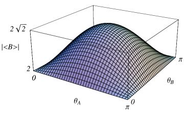
Figure 5.1: Plot of $C(\theta_{A},\theta_{B})=\max_{\rho\in\cal{D}}|\langle\mathcal{B}\rangle_{\rho}|$ as given in (5.14) for $0\leq\theta_{A},\theta_{B}\leq\pi$.

If both angles are chosen the same, i.e., $\theta_{A}=\theta_{B}:=\theta$, (5.14) simplifies to

$$C(\theta,\theta)=\sqrt{4+4\sin^{2}\theta},$$ (5.20)

which is plotted in Figure 5.3.

5.3.2 Separable qubit states

The set $\mathcal{D}_{\textrm{sep}}$ of separable two-qubit states is closed under local unitary transformations. Therefore, to find $\max_{\rho\in\mathcal{D}_{\textrm{sep}}}|\langle\mathcal{B}\rangle_{\rho}|$, we may consider the same choice of observables as before in (5.12) without loss of generality. Further, we only have to consider pure states and can take the state $|\,\Psi\rangle=|\,\psi_{1}\rangle|\,\psi_{2}\rangle$ with $|\,\psi_{1}\rangle=\cos\gamma_{1}e^{-i\phi_{1}/2}|\,0\rangle+\sin\gamma_{1}e^{i\phi_{1}/2}|\,1\rangle$ and $|\,\psi_{2}\rangle=\cos\gamma_{2}e^{-i\phi_{2}/2}|\,0\rangle+\sin\gamma_{2}e^{i\phi_{2}/2}|\,1\rangle$. We then obtain

$$\langle A\rangle_{\psi_{1}}=\sin 2\gamma_{1}\cos\phi_{1},\leavevmode\nobreak\ \leavevmode\nobreak\ \leavevmode\nobreak\ \langle A^{\prime}\rangle_{\psi_{1}}=\sin 2\gamma_{1}\cos(\phi_{1}-\theta_{A}),$$

$$\langle B\rangle_{{\psi_{2}}}=\sin 2\gamma_{2}\cos\phi_{2},\leavevmode\nobreak\ \leavevmode\nobreak\ \leavevmode\nobreak\ \langle B^{\prime}\rangle_{{\psi_{2}}}=\sin 2\gamma_{2}\cos(\phi_{2}-\theta_{B}).$$ (5.21)

Since $|\,\Psi\rangle$ is separable, we get $\langle A\otimes B\rangle_{\Psi}=\langle A\rangle_{{\psi_{1}}}\langle B\rangle_{{\psi_{2}}}$, etc., and the maximal expectation value of the CHSH operator becomes

$$D(\theta_{A},\theta_{B}) =\max_{{\Psi}}\,\langle\mathcal{B}\rangle_{\Psi}$$

$$=\max_{\gamma_{1},\gamma_{2},\phi_{1},\phi_{2}}\sin 2\gamma_{1}\sin 2\gamma_{2}[\cos\phi_{1}(\cos\phi_{2}+\cos(\phi_{2}-\theta_{B}))$$

$$\leavevmode\nobreak\ \leavevmode\nobreak\ \leavevmode\nobreak\ \leavevmode\nobreak\ \leavevmode\nobreak\ \leavevmode\nobreak\ \leavevmode\nobreak\ \leavevmode\nobreak\ \leavevmode\nobreak\ \leavevmode\nobreak\ \leavevmode\nobreak\ \leavevmode\nobreak\ \leavevmode\nobreak\ \leavevmode\nobreak\ \leavevmode\nobreak\ \leavevmode\nobreak\ \leavevmode\nobreak\ \leavevmode\nobreak\ \leavevmode\nobreak\ \leavevmode\nobreak\ \leavevmode\nobreak\ \leavevmode\nobreak\ \leavevmode\nobreak\ \leavevmode\nobreak\ +\cos(\phi_{1}-\theta_{A})(\cos\phi_{2}-\cos(\phi_{2}-\theta_{B}))].$$ (5.22)

This maximum is attained for $\gamma_{1}=\gamma_{2}=\pi/4$ and (5.22) reduces to:

$$D(\theta_{A},\theta_{B})=\max_{\phi_{1},\phi_{2}} \,\cos\phi_{1}(\cos\phi_{2}+\cos(\phi_{2}-\theta_{B}))$$

$$+\cos(\phi_{1}-\theta_{A})(\cos\phi_{2}-\cos(\phi_{2}-\theta_{B})).$$ (5.23)

A tedious but straightforward calculation yields that the maximum over $\phi_{1}$ and $\phi_{2}$ is given by

$$D(\theta_{A},\theta_{B})=\sqrt{2\big{(}1+\sqrt{1-\sin^{2}\theta_{A}\sin^{2}\theta_{B}}\,\big{)}}$$ (5.24)

The function (5.24) is plotted in Figure 5.2.

From this figure we conclude that the maximum of $|\langle\mathcal{B}\rangle_{\rho}|$ for separable two-qubit states becomes smaller and smaller when the angles approach orthogonality. For parallel and completely orthogonal settings we again retrieve the results of section 5.2.2.

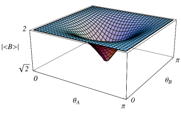
Figure 5.2: Plot of $D(\theta_{A},\theta_{B}):=\max_{\rho\in\cal{D}_{\textrm{sep}}}|\langle\mathcal{B}\rangle_{\rho}|$ as given in (5.24) for $0\leq\theta_{A},\theta_{B}\leq\pi$.

As a special case, suppose we choose $\theta_{A}=\theta_{B}:=\theta$. Then, (5.24) reduces to the much simpler expression

$$D(\theta,\theta)=|\cos\theta|+\sqrt{1+\sin^{2}\theta}.$$ (5.25)

This result strengthens the bound obtained previously by roy for this special case, which is:

$$D(\theta,\theta)\leq\left\{\begin{array}[]{ll}\sqrt{2}(|\cos\theta|+1),&|\cos\theta|\leq 3-2\sqrt{2},\\ 1+2\sqrt{|\cos\theta|}-|\cos\theta|,&\leavevmode\nobreak\ \leavevmode\nobreak\ \mathrm{otherwise}.\end{array}\right.$$ (5.28)

Both functions are shown in Figure 5.3.

Figure 5.3: Plot of the results (5.20) (dashed line) and (5.25) (uninterrupted line), and of the bound by roy given in (5.28) (dotted line).

5.4 Discussion

In this chapter we have given tight quantitative expressions for two trade-off relations. Firstly, between the degrees of local commutativity, as measured by the local angles $\theta_{A}$ and $\theta_{B}$, and the maximal degree of CHSH inequality violation, in the sense that if both local angles increase towards $\pi/2$ (i.e., the degree of local commutativity decreases), the maximum violation of the CHSH inequality increases. Secondly, a converse trade-off relation holds for separable two-qubit states: if both local angles increase towards $\pi/2$, the value attainable for the expectation of the CHSH operator decreases and thus the non-violation of the CHSH inequality increases. The extreme cases of these relations are obtained for anti-commuting local observables where the bounds of $2\sqrt{2}$ and $\sqrt{2}$ hold, which reproduces these results of the previous chapter. For the case of equal angles the trade-off relation for separable states strengthens a previous result of roy.

Our results are complementary to the well studied question what the maximum of the expectation value of the CHSH operator is when evaluated in a certain state (see e.g., GisiN; GISIN91; POPROHR). Here we have not focused on a certain given state, but instead on the observables chosen, i.e., we asked, independent of the specific state of the system, what the maximum of the expectation value of the CHSH operator is when using certain local observables. The answer found shows a diverging trade-off relation for the two classes of separable and non-separable two-qubit states.

Indeed, these two trade-off relations show that local non-commutativity has two diametrically opposed features: On the one hand, the choice of locally non-commuting observables is necessary to allow for any violation of the CHSH inequality in entangled states (a “more than classical” result). On the other hand, this very same choice of non-commuting observables implies a “less than classical” result for separable two-qubit states: For such states the correlations (in terms of $\langle\mathcal{B}\rangle_{\rho}$) obey a more stringent bound than allowed for by local hidden-variable theories, cf. the CHSH inequality (5.2).

These trade-off relations are useful for experiments aiming to detect entangled states. They have an experimental advantage above both Bell-type inequalities and entanglement witnesses as tests for two-qubit entanglement. This will be discussed next.

Figure 5.4: Violation factor $X$ (uninterrupted line) and $X_{\mathrm{CHSH}}$ (dashed line) for $\theta_{A}=\theta_{B}:=\theta$.

For comparison to the CHSH inequality as a test of entanglement, let us define the ’violation factor’ $X$ as the ratio $C(\theta_{A},\theta_{B})/D(\theta_{A},\theta_{B})$, i.e. the maximum correlation attained by entangled states divided by the maximum correlation attainable for separable states. In Figure (5.4) we have plotted this violation factor $X$ for the special case of equal angles, cf. (5.20) and (5.25) and compared it to the ratio by which these maximal correlations violate the CHSH inequality (5.2), i.e. $X_{\mathrm{CHSH}}:=C(\theta,\theta)/2$. Figure 5.4 shows that the violation factor $X$ is always higher than $X_{\rm CHSH}$ except when $\theta=0$. For angles $\theta\lesssim\pi/4$ these two factors differ only slightly, but the violation factor $X_{\mathrm{}}$ increases to $\sqrt{2}$ times the original factor $X_{\mathrm{CHSH}}$ when $\theta$ approaches $\pi/2$. Furthermore note that the factor $X_{\mathrm{}}$ increases more and more steeply, whereas $X_{\mathrm{CHSH}}$ increases less and less steeply. For the case of unequal angles the same features occur, as is evident from comparing Figures 5.1 and 5.2.

Therefore, the comparison of the correlation in entangled qubit states to the maximum correlation obtainable in separable states yields a stronger test for entanglement than violations of the CHSH inequality. Indeed, the violation factor may reach 2 instead of $\sqrt{2}$. This means that the separability inequality (5.10) detects more entangled states and tolerates greater noise robustness in detecting entanglement (cf. section 4.5). Clearly, the optimal case of this relation obtains when the local observables are exactly orthogonal to each other. On the other hand, in the case where at least one of the local pairs of observables are parallel, no improvement upon the CHSH inequality is obtained. But that case is trivial, i.e., no entangled state can violate either (5.2) or (5.10) in that case.

Other criteria for the detection of qubit entanglement than the CHSH inequality have been developed in the form of entanglement witnesses. In general, these criteria have two experimental drawbacks: (i) they are usually designed for the detection of a particular entangled state and hence require some a priori knowledge about the state, and (ii) they require the implementation of a specific set of local observables (e.g., locally orthogonal ones nonlinear; yu; zhang). The separability inequality (5.10) compares favorably on these two points, as we will discuss next.

In real experimental situations one might not be completely sure about which observables are being measured. For example, one might not be sure that the local angles are exactly orthogonal in the optimal setup. However, even in such cases, one might be reasonably sure that the angles are close to 90 degrees, e.g., that these angles certainly lie within some finite-sized interval $\epsilon$ around 90 degrees. In that case, the bound (5.10) for separable states would of course be higher than the optimal value of $\sqrt{2}$ and the increase depends on the size of the interval specified. But the trade-off relation presented in this letter tells us exactly how much higher the bound becomes as a function of the angles (e.g., $\theta=\pi/2\pm\epsilon$), so one can still obtain a relevant bound on $|\langle\mathcal{B}\rangle|$. One can thus still use it as a criterion for testing entanglement in the presence of some ignorance about the measured observables. Entanglement witnesses do not share this feature since no other trade-off relations have been obtained (at least to our knowledge) that quantify how the performance of the witness is changed when one allows for uncertainty in the observables that feature in the witness.

Note that for two qubits this result answers the question raised by nagataPRL where it was asked how separability inequalities for orthogonal observables could allow for some uncertainty $\epsilon$ in the orthogonality, i.e., allowing for $|\{A,A^{\prime}\}|\leq\epsilon$ (analogous for $B$, $B^{\prime}$). A further advantage of the separability inequalities (5.10) is that they are not state-dependent and are formulated in terms of locally measurable observables from the start, whereas it is usually the case (apart from a few simple cases) that constructions of entanglement witnesses involve some extremization procedure and are state-dependent. Furthermore, finding the decomposition of witnesses in terms of a few locally measurable observables is not always easy guhnewitness; guhnewitness1. However, it must be said that choosing the optimal set of observables in the separability inequalities for detecting a specific state of course also requires some prior knowledge of this state.

The results presented here only concern the case of two qubits and the bi-partite linear Bell-type inequality. It might prove useful to look for similar trade-off relations for nonlinear separability inequalities as well as for entanglement witnesses. Furthermore, it would be interesting to extend this analysis to the multi-partite Bell-type inequalities involving two dichotomous observables per party such as the Werner-Wolff-Żukowski-Brukner inequalities wernerwolf2; zukowskibrukner or the Mermin-type inequalities mermin. For the latter the situation for local anti-commutativity has already been investigated roy; nagataPRL; partsep, but for non-commuting observables that are not anti-commuting no results have yet been obtained.

III

Partial separability and
entanglement criteria for
multi-qubit quantum states

This chapter is largely based on (i) partsep, (ii) tothseev, and (iii) seevuff.

6.1 Introduction

The problem of characterizing entanglement for multi-partite quantum systems has recently drawn much attention. An important issue in this study is that, apart from the extreme cases of full separability and full entanglement of all particles in the system, one also has to face the intermediate situations in which only some subsets of particles are entangled and others not. The latter states are usually called ‘partially separable with respect to a specific partition’ or, more precisely, $k$-separable with respect to a specific partition if the $N$-partite system is separable into a specific partition of $k$ subsystems ($k\leq N$) duer2; duer22; duer; duer22; nagataPRL . The partial separability structure of multi-qubit states has been classified by duer2; duer22. This classification consists of a hierarchy of levels corresponding to the $k$-separable states for $k=1,\ldots N$, and within each level different classes are distinguished by specifying under which partitions of the system the state is $k$-separable or $k$-inseparable. As we shall argue, however, it is useful to extend this classification with one more class at each level $k$, since the notion of $k$-separability with respect to a specific partition does not exhaust all partial separability properties.

Several experimentally accessible conditions to characterize $k$-separable multi-qubit states have already been proposed, e.g., Bell-type inequalities laskowzukow; nagataPRL; roy; uffink; seevsvet; collins; gisin and, more generally, in terms of entanglement witnesses tothguhne2. However, these conditions address only part of the full classification since they do not distinguish between the various classes within a level. Here we derive separability conditions that do address the full classification of partial separability. This will be performed by generalizing the derivation of the two-qubit separability conditions of chapter 4 to the multi-qubit setting.

These new conditions take the form of inequalities that provide bounds on experimentally accessible correlations for the standard Bell-type experiments (involving at each site measurement of two dichotomic observables). These inequalities form a hierarchy with strong state-dependent bounds and numerical bounds that decrease by a factor of four for each level in the partial separability hierarchy. For the classes within a given level, the inequalities give state-dependent bounds, differing for each class. Violations of the inequalities provide strong sufficient criteria for various forms of non-separability and multi-qubit entanglement.

We next demonstrate the strength of these conditions in two ways: Firstly, by showing that they imply several other general experimentally accessible entanglement criteria, namely the fidelity criterion sackett; seevuff; fidelity, the Laskowski-Żukowski condition laskowzukow (with a strict improvement for $k=2,N$), and the Dür-Cirac criterion duer2; duer22. The first two are conditions for separability in general and the third is a condition for separability under specific partitions. We furthermore show that the new conditions imply the Mermin-type separability inequalities of nagataPRL; roy; uffink; seevsvet; collins; gisin. We also show that the latter are equivalent to the Laskowski-Żukowski separability condition.

Secondly, we compare the conditions to other state-specific multi-qubit entanglement criteria tothguhne2; guhne2007; chen both for their white noise robustness and for the number of measurement settings required in their implementation. In particular, we show (i) detection of bound entanglement for $N\geq 3$ with noise robustness for detecting the bound entangled states of duer22 that goes to $1$ for large $N$ (i.e., maximal noise robustness), (ii) detection of the four qubit Dicke state with noise robustness $0.84$ and $0.36$ for detecting it as entangled and fully entangled respectively, (iii) great noise and decoherence robustness noise2; noise in detecting entanglement of the $N$-qubit GHZ state where for colored noise and for decoherence due to dephasing the robustness for detecting full entanglement goes to $1$ for large $N$, and lastly, (iv) better white noise robustness than the stabilizer witness criteria of tothguhne2 for detecting the $N$-qubit GHZ states. In all these cases it is shown that only $N+1$ settings are needed.

Choosing the familiar Pauli matrices as the local orthogonal observables yields a convenient matrix element representation of the partial separability conditions. In this representation, the inequalities give specific bounds on the anti-diagonal matrix elements in terms of the diagonal ones. Further, some comments will be made along the way on how these results relate to the original purpose bell64 of Bell-type inequalities to test local hidden-variable models against quantum mechanics. Most notably, when the number of parties is increased, there is not only an exponentially increasing factor that separates the correlations allowed in maximally entangled states in comparison to those of local hidden-variable theories, but, surprisingly, also an exponentially increasing factor between the correlations allowed by LHV models and those allowed by non-entangled qubit states.

This chapter is structured as follows. In section 6.2 we define the relevant partial separability notions and extend the hierarchic partial separability classification of duer2; duer22. There we also introduce the notions of $k$-separable entanglement and of $m$-partite entanglement. Using these notions we investigate the relation between partial separability and multi-partite entanglement and show it to be non-trivial. The four experimentally accessible partial separability conditions are presented that are to be strengthened in the next section. In section 6.3 we derive the announced partial separability criteria for $N$ qubits in terms of experimentally accessible quantities. They provide the desired necessary conditions for the full hierarchic separability classification. From these we obtain the sufficient non-separability and entanglement criteria. In section 6.4 the experimental strength of these criteria is discussed. We end in section 6.5 with a discussion of the results obtained.

6.2 Partial separability and multi-partite
entanglement

In this section we introduce terminology and definitions to be used in later sections. We define the notions of $k$-separability, $\alpha_{k}$-separability, $k$-separable entanglement and $m$-partite entanglement and use these notions to capture aspects of the separability and entanglement structure in multi-partite states. We review the separability hierarchy introduced by duer2; duer22 and extend their classification. We also discuss four partial separability conditions known in the literature These conditions will be strengthened in 6.3.

6.2.1 Partial separability and the separability hierarchy

Consider an $N$-qubit system with Hilbert space $\mathcal{H}=\mathbb{C}^{2}\otimes\ldots\otimes\mathbb{C}^{2}$. Let $\alpha_{k}=(S_{1},\ldots,S_{k})$ denote a partition of $\{1,\ldots,N\}$ into $k$ disjoint nonempty subsets ($k\leq N$). Such a partition corresponds to a division of the system into $k$ distinct subsystems, also called a $k$-partite split duer2. A quantum state $\rho$ of this $N$-qubit system is $k$-separable under a specific $k$-partite split $\alpha_{k}$ duer2; duer22; duer; duer22; nagataPRL iff it is fully separable in terms of the $k$ subsystems in this split, i.e., iff

$$\rho=\sum_{i}p_{i}\otimes_{n=1}^{k}\rho_{i}^{S_{n}}\,,\leavevmode\nobreak\ \leavevmode\nobreak\ \leavevmode\nobreak\ \leavevmode\nobreak\ \leavevmode\nobreak\ p_{i}\geq 0,\leavevmode\nobreak\ \leavevmode\nobreak\ \sum_{i}p_{i}=1,$$ (6.1)

where $\rho^{S_{n}}$ is a state of the subsystem corresponding to $S_{n}$ in the split $\alpha_{k}$. We denote such states as $\rho\in{\cal D}_{N}^{\alpha_{k}}$ and also call them $\alpha_{k}$-separable, for short. Clearly, ${\cal D}_{N}^{\alpha_{k}}$ is a convex set. A state of the $N$-qubit system outside this set is called $\alpha_{k}$-inseparable.

More generally, a state $\rho$ is called $k$-separable laskowzukow; guhnetothbriegel; tothguhne1; acin; haffner, denoted as $\rho\in{\cal D}_{N}^{k\textrm{-sep}}$, iff there exists a convex decomposition

$$\rho=\sum_{j}p_{j}\otimes_{n=1}^{k}\rho^{S^{(j)}_{n}}\,,\leavevmode\nobreak\ \leavevmode\nobreak\ \leavevmode\nobreak\ \leavevmode\nobreak\ \leavevmode\nobreak\ p_{j}\geq 0,\leavevmode\nobreak\ \leavevmode\nobreak\ \sum_{j}p_{j}=1,$$ (6.2)

where each state $\otimes_{n=1}^{k}\rho^{S^{(j)}_{n}}$ is a tensor product of $k$ density matrices of the subsystems corresponding to some such partition $\alpha^{(j)}_{k}$, i.e., it factorizes under this split $\alpha_{k}^{(j)}$. In this definition, the partition may vary for each $j$, as long as it is a $k$-partite split, i.e., contains $k$ disjoint non-empty sets. Clearly ${\cal D}_{N}^{k\textrm{-sep}}$ is also convex; it is the convex hull of the union of all $\ {\cal D}_{N}^{\alpha_{k}}$ for fixed values of $k$ and $N$. States that are not $k$-separable will be called $k$-inseparable. Note that a $k$-separable state need not be $\alpha_{k}$-separable for any particular split $\alpha_{k}$. And even the converse implication need not hold: If a state is bi-separable under every bipartition, it does not have to be fully separable, as shown by the three-partite examples of bennett; eggeling; acin that give states that are bi-separable with respect to all bi-partite partitions, yet are not fully separable, i.e., they are three-inseparable. Similar observations (using different terminology) were obtained by guhnetothbriegel and tothguhne1, but below we will present a more systematic investigation.

The notion of $k$-separability naturally induces a hierarchic ordering of the $N$-qubit states. Indeed, the sequence of sets ${\cal D}_{N}^{k\textrm{-sep}}$ is nested: ${\cal D}_{N}^{N\textrm{-sep}}\subset{\cal D}_{N}^{(N-1)\textrm{-sep}}\subset\cdots\subset{\cal D}_{N}^{1\textrm{-sep}}$. In other words, $k$-separability implies $\ell$-separability for all $\ell\leq k$. We call a $k$-separable state that is not $(k+1)$-separable “$k$-separable entangled”. Thus, each $N$-qubit state can be characterized by the level $k$ for which it is $k$-separable entangled, and these levels provide a hierarchical ranking: at one extreme end are the $1$-separable entangled states which are fully entangled (e.g., the GHZ states), at the other end are the $N$-separable or fully separable states (e.g. product states or the “white noise state” $\leavevmode\hbox{\normalsize 1\kern-3.8pt\large 1}/2^{N}$).

Often, it is interesting to know how many qubits are entangled in a $k$-separable entangled state. However, this question does not have a unique answer. For example, take $N=4$ and $k=2$ (bi-separability). In this case two types of states may occur in the decomposition (6.2), namely $\rho^{\{ij\}}\otimes\rho^{\{kl\}}$ and $\rho^{\{i\}}\otimes\rho^{\{jkl\}}$ ($i,j,k,l=1,2,3,4$). A $2$-separable entangled four-partite state might thus be two- or three-partite entangled.

In general, an $N$-qubit state $\rho$ will be called $m$-partite entangled iff a decomposition of the state such as in (6.2) exists such that each subset $S^{(i)}$ contains at most $m$ parties, but no such decomposition is possible when all the $k$ subsets are required to contain less than $m$ parties seevuff. (guhnetothbriegel and tothguhne1 call this ‘not producible by $(m-1)$-partite entanglement’). It follows that a $k$-separable entangled state is also $m$-partite entangled, with $\lceil N/k\rfloor\leq m\leq N-k+1$. Here $\lceil N/k\rfloor$ denotes the smallest integer which is not less than $N/k$. Thus, a state that is $k$-separably entangled ($k<N$) is at least $\lceil N/k\rfloor$-partite entangled and might be up to $(N-k+1)$-partite entangled. Therefore, conditions that distinguish $k$-separability from $(k+1)$-separability also provide conditions for $m$-partite entanglement, but generally allowing a wide range of values of $m$. For example, for $N=100$ and $k=2$, $m$ might lie anywhere between 50 and 99.

Of course, a much tighter conclusion about $m$-partite entanglement can be drawn if we know exactly under which splits the state is separable. This is why the notion of $\alpha_{k}$-separability is helpful, since it provides these finer distinctions. For example, suppose that a 100-qubit state is separable under the bi-partite split $(\{1\},\{2,\ldots 100\})$ but under no other bi-partite split. This state would then be $2$-separable (bi-separable) but now we could also infer that $m=99$. On the other hand, if the state were only separable under the split $\{1,\ldots 50\},\{51,\ldots 100\}$, it would still be bi-separable, but only $m$-partite entangled for $m=50$.

duer2 provided such a fine-grained classification of $N$-qubit states by considering their separability or inseparability under all $k$-partite splits. Let us introduce this classification (with a slight extension) by means of the example of three qubits, labeled as $a,b,c$.

Class 3. Starting with the lowest level $k=3$, there is only one 3-partite split, $a$-$b$-$c$, and consequently only one class to be distinguished at this level , i.e. ${\cal D}_{3}^{a\textrm{-}b\textrm{-}c}$. This set coincides with ${\cal D}^{3\textrm{-sep}}_{3}$.

Classes 2.1—2.8 Next, at level $k=2$, there are three bi-partite splits: $a$-$(bc)$, $b$-$(ac)$ and $c$-$(ab)$ which define the sets ${\cal D}_{3}^{a\textrm{-}(bc)}$, ${\cal D}_{3}^{b\textrm{-}(ac)}$, and ${\cal D}_{3}^{c\textrm{-}(ab)}$. One can further distinguish classes defined by all logical combinations of separability and inseparability under these splits, i.e. all the set-theoretical intersections and complements shown in Figure 1. This leads to classes 2.2 – 2.8. duer2; duer22 showed that all these classes are non-empty. To these, we add one more class 2.1: the set of bi-separable states that are not separable under any split. As we have seen, this set is non-empty too.

Class 1. Finally, at level $k=1$ there is again only one (trivial) split $(abc)$, and thus only one class, consisting of all the fully entangled states, i.e., ${\cal D}_{3}^{1\textrm{-sep}}\setminus{\cal D}_{3}^{2\textrm{-sep}}$.

Figure 6.1: Schematic representation of the 10 partial separability classes of three-qubit states

We feel that the above extension is desirable since otherwise the Dür-Cirac classification would not distinguish between class 2.1 and class 1. However, states in class 2.1 are simply convex combinations of states that are bi-separable under different bi-partite splits. Such states can be realized by mixing the bi-separable states, and are conceptually different from the fully inseparable states of class 1.

This three-partite example serves to illustrate how the Dür-Cirac separability classification works for general $N$. Level $k$ ($1\leq k\leq N$) of the separability hierarchy consists of all $k$-separable entangled states. Each level is further divided into distinct classes by considering all logically possible combinations of separability and inseparability under the various $k$-partite splits. The number of such classes increases rapidly with $N$, and therefore we will not attempt to list them. In general, all such classes may be non-empty. As an extension of the Dür-Cirac classification, we distinguish at each level $1<k<N$ one further class, consisting of $k$-separable entangled states that are not separable under any $k$-partite split.

In order to find relations between these classes, the notion of a contained split is useful duer2. A $k$-partite split $\alpha_{k}$ is contained in a $l$-partite split $\alpha_{l}$, denoted as $\alpha_{k}\prec\alpha_{\ell}$, if $\alpha_{l}$ can be obtained from $\alpha_{k}$ by joining some of the subsets of $\alpha_{k}$. The relation $\prec$ defines a partial order between splits at different levels. This partial order is helpful because $\alpha_{k}$-separability implies $\alpha_{\ell}$-separability of all splits $\alpha_{\ell}$ containing $\alpha_{k}$. We will use this implication below to obtain conditions for separability of a $k$-partite split at level $k$ from such conditions on all $(k-1)$-partite splits at level $k-1$ this $k$-partite split is contained in. One can thus construct separability conditions for all classes at higher levels from the separability conditions for classes at level $k=2$. Conditions at a lower level thus imply conditions at a higher level.

The multi-partite entanglement properties of $k$-separable or $\alpha_{k}$-separable states are subtle, as can be seen from the following examples.

(i) mixing states does not conserve $m$-partite entanglement. Take $N=3$, then mixing the $2$-partite entangled $2$-separable states $|\,0\rangle\otimes(|\,00\rangle+|\,11\rangle)/\sqrt{2}$ and $|\,0\rangle\otimes(|\,00\rangle-|\,11\rangle)/\sqrt{2}$ with equal weights gives a $3$-separable state $(|\,000\rangle\langle\,000|+|\,011\rangle\langle\,011|)/2$.

(ii) an $N$-partite state can be $m$-partite entangled ($m<N$) even if it has no $m$-partite subsystem whose (reduced) state is $m$-partite entangled seevuff; guhnetothbriegel. Such states are said to have irreducible $m$-partite entanglement. Thus, a state of which some reduced state is $m$-partite entangled is itself at least $m$-partite entangled, but the converse need not be true.

(iii) consider a bi-separable entangled state that is only separable under the bi-partite split $(\{1\},\{2,\ldots,N\})$. One cannot infer that the subsystem $\{2,\ldots,N\}$ is $(N-1)$-partite entangled. A counterexample is the three-qubit state $\rho=(|\,0\rangle\langle\,0|\otimes P^{(bc)}_{-}+|\,1\rangle\langle\,1|\otimes P^{(bc)}_{+})/2$ which is bi-separable only under the partition $a\textrm{-}(bc)$, and thus bi-partite entangled, but has no bi-partite subsystem whose reduced state is entangled. Here $P^{(bc)}_{+}$ and $P^{(bc)}_{-}$ denote projectors on the Bell states $|\,\psi^{\pm}\rangle=\frac{1}{\sqrt{2}}(|\,01\rangle\pm|\,10\rangle)$ for parties $b$ and $c$, respectively.

(iv) a state that is inseparable under all splits but which is not fully inseparable (i.e., $\rho\in{\cal D}^{k\textrm{-sep}}_{N}$ with $k>1$ and $\rho\notin\cup_{\alpha_{k}}{\cal D}^{\alpha_{k}}_{N},\leavevmode\nobreak\ \forall\,\alpha_{k},k$) might still have all forms of $m$-partite entanglement apart from full entanglement, i.e., it could be $m$-partite entangled with $2\leq m\leq N-1$. Thus the state could even have $m$-partite entanglement as low as $2$-partite entanglement, although it is inseparable under all splits. For example, tothguhne1 consider a mixture of two $N$-partite states where each of them is $(\lceil N/2\rfloor)$- separable according to different splits. This mixed state is by construction $(\lceil N/2\rfloor)$- separable, not bi-separable under any split, yet only $2$-partite entangled. See also the example in footnote 2 which is $(N-1)$-separable and only $2$-partite entangled.

(v) Lastly, $N$-partite fully entangled states exist where no $m$-partite reduced state is entangled (such as $N$-qubit GHZ state) and also where all $m$-partite reduced states are entangled (such as the $N$-qubit W-states) durR.

These examples serve to emphasize that one should be very cautious in inferring the existence of entanglement in subsystems of a larger system which is known to be $m$-partite entangled or $k$-separable entangled for some specific value of $m$ and $k$.

6.2.2 Separability Conditions

We now review four separability conditions for qubits, which will all be strengthened in the next section. These are necessary conditions for states to be $k$-separable, $2$-separable, and $\alpha_{k}$-separable respectively.

(I) laskowzukow showed that for any $k$-separable $N$-qubit state $\rho$ the anti-diagonal matrix elements (denoted by $\rho_{j,\bar{\jmath}}$, where $\bar{\jmath}=d+1-j$, $d=2^{N}$ ) must satisfy

$$\max_{j}|\rho_{j,\bar{\jmath}}|\leq\big{(}\frac{1}{2}\big{)}^{k},\leavevmode\nobreak\ \leavevmode\nobreak\ \leavevmode\nobreak\ \forall\rho\in{\cal D}^{k\textrm{-sep}}_{N}.$$ (6.3)

This condition can be easily proven by the observation that for any density matrix to be physically meaningful its anti-diagonal matrix elements must not exceed $1/2$. Therefore, anti-diagonal elements of a product of $k$ density matrices cannot be greater than $(1/2)^{k}$. For pure states this can be checked directly and by convexity, this results then holds all $k$-separable states. Note that this condition is not basis dependent.

It follows from (6.3) that if the anti-diagonal matrix elements of state $\rho$ obey

$$\big{(}\frac{1}{2}\big{)}^{k}\geq\max_{j}|\rho_{j,\bar{\jmath}}|>\big{(}\frac{1}{2}\big{)}^{k+1},$$ (6.4)

then $\rho$ is at most $k$-separable, i.e., $k$-separable entangled, and thus at least $m$-partite entangled, with $m\geq\lceil N/k\rfloor$.

The partial separability condition (6.3) does not yet explicitly refer to directly experimentally accessible quantities. However, in the next section we will rewrite this condition in terms of expectation values of local observables, and show that they are equivalent to Mermin-type separability inequalities.

(II) Mermin-type separability inequalities nagataPRL; roy; uffink; seevsvet; gisin; collins. Consider the familiar CHSH operator for two qubits (labeled as $a$ and $b$) which is defined by:

$$M^{(2)}:=X_{a}\otimes X_{b}+X_{a}\otimes Y_{b}+Y_{a}\otimes X_{b}-Y_{a}\otimes Y_{b}.$$ (6.5)

Here, $X_{a}$ and $Y_{a}$ denote two spin observables on the Hilbert spaces ${\cal H}_{a}$ and ${\cal H}_{b}$ of qubit $a$, and $b$. The so-called Mermin operator mermin is a generalization of this operator to $N$ qubits (labeled as $(a,b,\ldots n)$), defined by the recursive relation:

$$M^{(N)}:=\frac{1}{2}M^{(N-1)}\otimes(X_{n}+Y_{n})+\frac{1}{2}M^{\prime(N-1)}\otimes(X_{n}-Y_{n}),$$ (6.6)

where $M^{\prime}$ is the same operator as $M$ but with all $X$’s and $Y$’s interchanged.

In the special case where, for each qubit, the spin observables $X$ and $Y$ are orthogonal, i.e. $\{X_{i},Y_{i}\}=0$ for $i\in\{a,\ldots n\}$, nagataPRL obtained the following $k$-separability conditions:

$$\langle M^{(N)}\rangle^{2}+\langle M^{\prime(N)}\rangle^{2}\leq 2^{(N+3)}\big{(}\frac{1}{4}\big{)}^{k},\leavevmode\nobreak\ \leavevmode\nobreak\ \forall\rho\in{\cal D}_{N}^{k\textrm{-sep}}.$$ (6.7)

As just mentioned, the next section will show that these inequalities are equivalent to the Laskowski-Żukowski inequalities. The quadratic inequalities (6.7) also imply the following sharp linear Mermin-type inequality for $k$-separability:

$$|\langle M^{(N)}\rangle|\leq 2^{(\frac{N+3}{2})}\big{(}\frac{1}{2}\big{)}^{k},\leavevmode\nobreak\ \leavevmode\nobreak\ \forall\rho\in{\cal D}_{N}^{k\textrm{-sep}}.$$ (6.8)

For $k=N$ inequality (6.8) reproduces a result obtained by roy.

(III). The fidelity $F(\rho)$ of a $N$-qubit state $\rho$ with respect to the generalized $N$-qubit GHZ state $|\,\Psi_{{\rm GHZ},\alpha}^{N}\rangle:=(|\,0\rangle^{\otimes N}+e^{i\alpha}|\,1\rangle^{\otimes N})/\sqrt{2}$ ($\alpha\in\mathbb{R}$) is defined as

$$F(\rho):=\max_{\alpha}\langle\Psi_{{\rm GHZ},\alpha}^{N}|\rho|\Psi_{{\rm GHZ},\alpha}^{N}\rangle=\frac{1}{2}(\rho_{1,1}+\rho_{d,d})+|\rho_{1,d}|,$$ (6.9)

The fidelity condition sackett; seevuff; fidelity (also known as the projection-based witness tothguhne2) says that for all bi-separable $\rho$:

$$F(\rho)\leq 1/2,\leavevmode\nobreak\ \leavevmode\nobreak\ \leavevmode\nobreak\ \forall\rho\in{\cal D}_{N}^{2\textrm{-sep}}.$$ (6.10)

In other words, $F(\rho)>1/2$ is a sufficient condition for full $N$-partite entanglement. An equivalent formulation of (6.10) is:

$$2|\rho_{1,d}|\leq\sum_{j\neq 1,d}\rho_{j,j},\leavevmode\nobreak\ \leavevmode\nobreak\ \leavevmode\nobreak\ \forall\rho\in{\cal D}^{2\textrm{-sep}}_{N}.$$ (6.11)

Of course, analogous conditions may be obtained by replacing $|\,\Psi_{{\rm GHZ},\alpha}^{N}\rangle$ in the definition (6.9) by any other maximally entangled state fidelity; nagata2002. Exploiting this feature, one can reformulate (6.11) in a basis-independent form:

$$2\max_{j}|\rho_{j,\bar{\jmath}}|\leq\sum_{i\neq j,\bar{\jmath}}\rho_{i,i},\leavevmode\nobreak\ \leavevmode\nobreak\ \leavevmode\nobreak\ \forall\rho\in{\cal D}^{2\textrm{-sep}}_{N}.$$ (6.12)

Note that in contrast to the Laskowski-Żukowski condition and the Mermin-type separability inequalities, the fidelity condition does not distinguish bi-separability and other forms of $k$-separability. Indeed, a fully separable state (e.g. $|\,0^{\otimes N}\rangle$ can already attain the value $F(\rho)=1/2$. Thus, the fidelity condition only distinguishes full inseparability (i.e., $k=1$) from other types of separability ($k\geq 2$). However, as will be shown in the next section, violation of the fidelity condition yields a stronger test for full entanglement than violation of the Laskowski-Żukowski condition.

(IV) The Dür-Cirac depolarization method duer; duer2 gives necessary conditions for partial separability under specific bi-partite splits. It uses a two-step procedure in which a general state $\rho$ is first depolarized to become a member of a special family of states, called $\rho_{N}$, after which this depolarized state is tested for $\alpha_{2}$-separability under a bi-partite split $\alpha_{2}$. If the depolarized state $\rho_{N}$ is not separable under $\alpha_{2}$, then neither is the original state $\rho$, but not necessarily vice versa since the depolarization process can decrease inseparability.

The special family of states $\rho_{N}$ is given by

$$\rho_{N}=\lambda_{0}^{+}|\,\psi_{0}^{+}\rangle\langle\,\psi_{0}^{+}|+\lambda_{0}^{-}|\,\psi_{0}^{-}\rangle\langle\,\psi_{0}^{-}|+\sum_{j=1}^{2^{N-1}-1}\lambda_{j}(|\,\psi_{j}^{+}\rangle\langle\,\psi_{j}^{+}|+|\,\psi_{j}^{-}\rangle\langle\,\psi_{j}^{-}|),$$ (6.13)

with the so-called orthonormal GHZ-basis $|\,\psi_{j}^{\pm}\rangle=\frac{1}{\sqrt{2}}|\,j0\rangle\pm|\,j^{\prime}1\rangle)$, where $j=j_{1}j_{2}\ldots j_{N-1}$ is in binary notation (i.e., a string of $N-1$ bits), and $j^{\prime}$ means a bit-flip of $j$: $j^{\prime}=j^{\prime}_{1}j^{\prime}_{2}\ldots j^{\prime}_{N-1}$, with $j^{\prime}_{i}=1,0$ if $j_{i}=0,1$. The depolarization process does not alter the values of $\lambda_{0}^{\pm}=\langle\,\psi_{0}^{\pm}|\rho|\,\psi_{0}^{\pm}\rangle$ and of $\lambda_{j}=(\langle\,\psi_{j}^{+}|\rho|\,\psi_{j}^{+}\rangle+\langle\,\psi_{j}^{-}|\rho|\,\psi_{j}^{-}\rangle)/2$ of the original state $\rho$. The values of $j=j_{1}j_{2}\ldots j_{N-1}$ can be used to label the various bi-partite splits by stipulating that $j=j_{1}j_{2}\ldots j_{N-1}$, $j_{n}=0,(1)$ corresponds to the $n$-th qubit belonging (not belonging) to the same subset as the last qubit. For example, the splits $a$-$(bc)$, $b$-$(ac)$, $c$-$(ab)$ have labels $j=10,01,11$ respectively.

The Dür-Cirac condition duer2 says that a state $\rho$ is separable under a specific bi-partite split $j$ if

$$|\lambda_{0}^{+}-\lambda_{0}^{-}|\leq 2\lambda_{j}\leavevmode\nobreak\ \leavevmode\nobreak\ \leavevmode\nobreak\ \Longleftrightarrow\leavevmode\nobreak\ \leavevmode\nobreak\ \leavevmode\nobreak\ 2|\rho_{1,d}|\leq\rho_{l,l}+\rho_{\bar{l},\bar{l}},\leavevmode\nobreak\ \leavevmode\nobreak\ \leavevmode\nobreak\ \leavevmode\nobreak\ \leavevmode\nobreak\ \forall\rho\in{\cal D}^{j}_{N},\leavevmode\nobreak\ \leavevmode\nobreak\ \leavevmode\nobreak\ \bar{l}=d+1-l,$$ (6.14)

For the states (6.13) this condition is in fact necessary and sufficient. In the right-hand side of the second inequality of (6.14) $l$ is determined from $j$ using Tr$[\rho|\,\psi_{j}^{+}\rangle\langle\,\psi_{j}^{+}|+|\,\psi_{j}^{-}\rangle\langle\,\psi_{j}^{-}|]=\rho_{l,l}+\rho_{\bar{l},\bar{l}}$.

Separability conditions for multi-partite splits are constructed from the conditions (6.14) by means of the partial order $\prec$ of containment. As mentioned above, if a state is $\alpha_{k}$-separable, then it is also $\alpha_{2}$-separable for all bi-partite splits $\alpha_{k}\prec\alpha_{2}$. Therefore, the conjunction of all $\alpha_{2}$-separability conditions must hold for such a state.

Note that if $|\lambda_{0}^{+}-\lambda_{0}^{-}|>2\max_{j}\lambda_{j}$, the state is inseparable under all bi-partite splits, but this does not imply that it is fully inseparable (cf. footnote 2). Indeed, this feature also exists for states of the form (6.13) as the following example shows. Take the following two members of the family (6.13) for $N=3$: for $\rho_{3}^{i}$ we choose $\lambda_{0}^{+}=1/2$, $\lambda_{0}^{-}=0$, $\lambda_{01}=0$, $\lambda_{10}=1/4$, $\lambda_{11}=0$, and for $\rho_{3}^{ii}$ : $\lambda_{0}^{+}=1/2$, $\lambda_{0}^{-}=0$, $\lambda_{01}=0$, $\lambda_{10}=0$, $\lambda_{11}=1/4$. It follows from condition (6.14) that $\rho_{3}^{i}$ is separable under split $a$-$(bc)$ and inseparable under other splits, while $\rho_{3}^{ii}$ is separable under the split $c$-$(ab)$ and inseparable under any other split. Now form a convex mixture of these two states: $\tilde{\rho}_{3}=\alpha\rho_{3}^{i}+\beta\rho_{3}^{ii}$ with $\alpha+\beta=1$ and $\alpha,\leavevmode\nobreak\ \beta\in(0,1)$. This state $\tilde{\rho}_{3}$ is still of the form (6.13), so that we can again apply condition (6.14) to conclude that $\tilde{\rho}_{3}$ is not separable under any bi-partite split, yet bi-separable by construction.

In the next section we give necessary conditions for $k$-separability and $\alpha_{k}$-separability that are stronger than the Laskowski-Żukowski condition (for $k=2,N$), the fidelity condition and the Dür-Cirac condition.

6.3 Deriving new partial separability conditions

In this section we present $k$-separability conditions for all levels and classes in the hierarchic classification of $N$-qubit states. Violations of the conditions give strong criteria for specific forms of non-separability and $m$-partite entanglement. The starting point will be the two-qubit results of chapter 4, whose result we rehearse here for both convenience and for introducing the notation to be used in this chapter. We next move on to the slightly more complicated case of three qubits, for which explicit separability conditions are given for each of the 10 classes in the separability hierarchy that were depicted in Figure 6.1. Finally, the case of $N$-qubits is treated by a straightforward generalization.

6.3.1 Two-qubit case: setting the stage

For two-qubit systems the separability hierarchy is very simple: there is only one possible split, and consequently just one class at each of the two levels $k=1$ and $k=2$, i.e., states are either inseparable (entangled) or separable.

Consider a system composed of a pair of qubits in the familiar setting of two distant sites, each receiving one of the two qubits, and where, at each site, a measurement of either of two spin observables is made. We will focus on the special case that these local spin observables are mutually orthogonal. Let $(X^{(1)}_{a},Y^{(1)}_{a},Z^{(1)}_{a})$ denote three orthogonal spin observables on qubit $a$, and $(X^{(1)}_{b},Y^{(1)}_{b},Z^{(1)}_{b})$ on qubit $b$. (The superscript $1$ denotes that we are dealing with single-qubit operators.) A familiar choice for the orthogonal triples $\{X^{(1)},Y^{(1)},Z^{(1)}\}$ are the Pauli matrices $\{\sigma_{x},\sigma_{y},\sigma_{z}\}$. But note that the choice of the two sets need not coincide. We further define $I^{(1)}_{a,b}:=\mathds{1}$. For all single-qubit pure states $|\,\psi\rangle$ we have

$$\langle X^{(1)}_{j}\rangle_{\psi}^{2}+\langle Y^{(1)}_{j}\rangle_{\psi}^{2}+\langle Z^{(1)}_{j}\rangle_{\psi}^{2}=\langle I^{(1)}_{j}\rangle_{\psi}^{2},\leavevmode\nobreak\ \leavevmode\nobreak\ \leavevmode\nobreak\ j=a,b,$$ (6.15)

and for mixed states $\rho$

$$\langle X^{(1)}_{j}\rangle^{2}+\langle Y^{(1)}_{j}\rangle^{2}+\langle Z^{(1)}_{j}\rangle^{2}\leq\langle I^{(1)}_{j}\rangle^{2},\leavevmode\nobreak\ \leavevmode\nobreak\ \leavevmode\nobreak\ j=a,b.$$ (6.16)

We write $X_{a}X_{b}$ or even $XX$ etc.  as shorthand for $X_{a}\otimes X_{b}$ and $\langle XX\rangle:=\mathrm{Tr}[\rho X_{a}\otimes X_{b}]$ for the expectation value in a general state $\rho$, and $\langle XX\rangle_{\Psi}:=\langle\,\Psi|X_{a}\otimes X_{b}|\,\Psi\rangle$ for the expectation in a pure state $|\,\Psi\rangle$.

So, let two triples of locally orthogonal observables be given, denoted as $\{X^{(1)}_{a},Y^{(1)}_{a},Z^{(1)}_{a}\}$ and $\{X^{(1)}_{b},Y^{(1)}_{b},Z^{(1)}_{b}\}$, where $a,b$ label the different qubits. We further introduce two sets of four two-qubit operators on $\mathcal{H}=\mathbb{C}^{2}\otimes\mathbb{C}^{2}$, labeled by the subscript $x=0,1$:

$$X_{0}^{(2)} :=\frac{1}{2}(X^{(1)}X^{(1)}-Y^{(1)}Y^{(1)}) X_{1}^{(2)} :=\frac{1}{2}(X^{(1)}X^{(1)}+Y^{(1)}Y^{(1)})$$

$$Y_{0}^{(2)} :=\frac{1}{2}(Y^{(1)}X^{(1)}+X^{(1)}Y^{(1)}) {Y}_{1}^{(2)} :=\frac{1}{2}(Y^{(1)}X^{(1)}-X^{(1)}Y^{(1)})$$

$$Z_{0}^{(2)} :=\frac{1}{2}(Z^{(1)}I^{(1)}+I^{(1)}Z^{(1)}) {Z}_{1}^{(2)} :=\frac{1}{2}(Z^{(1)}I^{(1)}-I^{(1)}Z^{(1)})$$

$$I_{0}^{(2)} :=\frac{1}{2}(I^{(1)}I^{(1)}+Z^{(1)}Z^{(1)}) {I}_{1}^{(2)} :=\frac{1}{2}(I^{(1)}I^{(1)}-Z^{(1)}Z^{(1)}).$$ (6.17)

Here, the superscript label indicates that we are dealing with two-qubit operators. Later on, $X_{x}^{(2)}$ will sometimes be notated as $X_{x,ab}^{(2)}$, and similarly for $Y_{x}^{(2)}$, $Z_{x}^{(2)}$ and $I_{x}^{(2)}$. This more extensive labeling will prove convenient for the multi-qubit generalization. Note that $(X^{(2)}_{x})^{2}=(Y^{(2)}_{x})^{2}=(Z^{(2)}_{x})^{2}=(I^{(2)}_{x})^{2}=I^{(2)}_{x}$ for $x=0,1$, and that all eight operators mutually anti-commute. Furthermore, if the orientations of the two triples is the same, these two sets form representations of the generalized Pauli group, i.e., they have the same commutation relations as the Pauli matrices on $\mathbb{C}^{2}$, i.e.: $[X_{x}^{(2)},Y_{x}^{(2)}]=2iZ_{x}^{(2)}$, etc.  and

$$\langle X_{x}^{(2)}\rangle^{2}+\langle Y_{x}^{(2)}\rangle^{2}+\langle Z_{x}^{(2)}\rangle^{2}\leq\langle I_{x}^{(2)}\rangle^{2},\leavevmode\nobreak\ \leavevmode\nobreak\ \leavevmode\nobreak\ x\in\{0,1\},$$ (6.18)

with equality only for pure states. Note that we can rewrite the CHSH inequality (4.2) in terms of these observables as: $|\langle X_{0}^{(2)}+Y_{0}^{(2)}\rangle|\leq 1,\leavevmode\nobreak\ \forall\rho\in{\cal D}^{2\textrm{-sep}}_{2}$.

Let us now consider the separability inequalities of chapter 4. In terms of the observables of (6.17) the separability inequality of (4.9) becomes:

$$\langle X_{x}^{(2)}\rangle^{2}+\langle Y_{x}^{(2)}\rangle^{2}\leq\frac{1}{4}(\langle I_{a}^{(1)}\rangle-\langle Z^{(1)}_{a}\rangle^{2})(\langle I_{b}^{(1)}\rangle-\langle Z^{(1)}_{b}\rangle^{2}),\leavevmode\nobreak\ \leavevmode\nobreak\ \leavevmode\nobreak\ \forall\rho\in{\cal D}^{2\textrm{-sep}}_{2}.$$ (6.19)

Since $(\langle X_{0}^{(2)}+Y_{0}^{(2)}\rangle)^{2}+(\langle X_{0}^{(2)}-Y_{0}^{(2)}\rangle)^{2}=2(\langle X_{0}^{(2)}\rangle^{2}+\langle Y_{0}^{(2)}\rangle^{2})$ we obtain from (6.19) that $|\langle X_{0}^{(2)}+Y_{0}^{(2)}\rangle|\leq\sqrt{1/2}$, thereby reproducing (4.10) which shows the strengthening of the CHSH separability inequality by a factor $\sqrt{2}$.

The separability condition of (6.19) can be strengthened even further as was done in section 4.4 to produce (4.35). In terms of the notation of this chapter this separability condition is

$$\max\left\{\begin{array}[]{c}\langle X_{0}^{(2)}\rangle^{2}+\langle Y_{0}^{(2)}\rangle\\ \langle X_{1}^{(2)}\rangle^{2}+\langle Y_{1}^{(2)}\rangle\end{array}\right\}\leq\min\left\{\begin{array}[]{c}\langle I_{0}^{(2)}\rangle^{2}-\langle Z_{0}^{(2)}\rangle^{2}\\ \langle I_{1}^{(2)}\rangle^{2}-\langle Z_{1}^{(2)}\rangle^{2}\end{array}\right\}\leq\frac{1}{4},\leavevmode\nobreak\ \leavevmode\nobreak\ \forall\rho\in{\cal D}^{2\textrm{-sep}}_{2}.$$ (6.24)

If we leave out the upper bound of $1/4$ in (6.24), then of the four inequalities in (6.24) two are trivially true for all states, whether separable or not, and the other two in fact provide the separability criteria. Which two of the four depends on the orientation of the local orthogonal observables. Let us choose the orientations for both parties to be the same, then the non-trivial inequalities are $\langle X_{0}^{(2)}\rangle^{2}+\langle Y_{0}^{(2)}\rangle\leq\langle I_{1}^{(2)}\rangle^{2}-\langle Z_{1}^{(2)}\rangle^{2}$ and $\langle X_{1}^{(2)}\rangle^{2}+\langle Y_{1}^{(2)}\rangle\leq\langle I_{0}^{(2)}\rangle^{2}-\langle Z_{0}^{(2)}\rangle^{2}$. Choosing the orientations to be different gives the other two non-trivial inequalities.

To conclude this section we give an explicit form of the separability inequalities (6.24) by choosing the Pauli matrices $\{\sigma_{x},\sigma_{y},\sigma_{z}\}$ for both triples $\{X^{(1)}_{a}\!,Y^{(1)}_{a}\!,Z^{(1)}_{a}\}$ and $\{X^{(1)}_{b}\!,Y^{(1)}_{b}\!,Z^{(1)}_{b}\}$. This choice enables us to write the inequalities (6.24) in terms of the density matrix elements on the standard $z$-basis $\{|\,00\rangle,|\,01\rangle,|\,10\rangle,|\,11\rangle\}$, labeled here as $\{|\,1\rangle,|\,2\rangle,|\,3\rangle,|\,4\rangle\}$. This choice of observables yields $\langle X_{0}^{(2)}\rangle=2\mathrm{Re}\,\rho_{1,4}$, $\langle Y_{0}^{(2)}\rangle=-2\mathrm{Im}\,\rho_{1,4}$, $\langle I_{0}^{(2)}\rangle=\rho_{1,1}+\rho_{4,4}$, $\langle Z_{0}^{(2)}\rangle=\rho_{1,1}-\rho_{4,4}$, $\langle X_{1}^{(2)}\rangle=2\mathrm{Re}\,\rho_{2,3}$, $\langle Y_{1}^{(2)}\rangle=-2\mathrm{Im}\,\rho_{2,3}$, $\langle I_{1}^{(2)}\rangle=\rho_{2,2}+\rho_{3,3}$, $\langle Z_{1}^{(2)}\rangle=\rho_{2,2}-\rho_{3,3}$. So, in this choice, we can write (6.24) as:

$$\max\{|\rho_{1,4}|^{2},\,|\rho_{2,3}|^{2}\}\leq\min\{\rho_{1,1}\rho_{4,4},\,\rho_{2,2}\rho_{3,3}\}\leq\frac{1}{16},\leavevmode\nobreak\ \leavevmode\nobreak\ \leavevmode\nobreak\ \leavevmode\nobreak\ \rho\in{\cal D}^{2\textrm{-sep}}_{2}.$$ (6.25)

In the form (6.25), it is easy to compare the result to the separability conditions reviewed in subsection II.B. Assume for simplicity that $|\rho_{1,4}|$ is the largest of all the anti-diagonal elements $|\rho_{j\bar{\jmath}}|$. Then, for $\rho\in{\cal D}^{2\textrm{-sep}}_{2}$, and using $\langle M^{(2)}\rangle^{2}+\langle M^{\prime(2)}\rangle^{2}=8(\langle X_{0}^{(2)}\rangle^{2}+\langle Y_{0}^{(2)}\rangle^{2})$ the Mermin-type separability inequality (6.7) becomes $|\rho_{1,4}|^{2}\leq 1/16$, which is equivalent to the Laskowski-Żukowski condition $|\rho_{1,4}|\leq 1/4$; the fidelity/Dür-Cirac conditions read: $2|\rho_{1,4}|\leq\rho_{2,2}+\rho_{3,3}$; and the condition (6.25): $|\rho_{1,4}|^{2}\leq\rho_{2,2}\rho_{3,3}$. Using the trivial inequality $(\sqrt{\rho_{22}}-\sqrt{\rho_{33}})^{2}\geq 0\Longleftrightarrow 2\sqrt{\rho_{2,2}\rho_{3,3}}\leq\rho_{2,2}+\rho_{3,3}$, we can then write the following chain of inequalities

$$4|\rho_{1,4}|-(\rho_{1,1}+\rho_{4,4})\overset{A}{\leq}2|\rho_{1,4}|\overset{\textrm{sep}}{\leq}2\sqrt{\rho_{2,2}\rho_{3,3}}\overset{A}{\leq}\rho_{2,2}+\rho_{3,3}\,,$$ (6.26)

where we used the symbols $\overset{A}{\leq}$ and $\overset{\textrm{sep}}{\leq}$ to denote inequalities that hold for all states, and for the separability condition (6.25) respectively.

The Laskowski-Żukowski condition is then recovered by comparing the first and fourth expressions in this chain, the fidelity/ Dür-Cirac conditions by comparing the second and fourth expression, and a new condition – not previously mentioned – can be obtained by comparing the first and third term, whereas condition (6.25), i.e. the comparison between the second and third expression in (6.26), is the strongest inequality in this chain, and thus implies and strengthens all of these other conditions.

6.3.2 Three-qubit case

We now derive separability conditions that distinguish the $10$ classes in the $3$-qubit classification of section 6.2.1 by generalizing the method of section 6.3.1. To begin with, define four sets of three-qubit observables from the two-qubit operators (6.17):

$$X_{0}^{(3)} :=\frac{1}{2}\,(X^{(1)}X^{(2)}_{0}-Y^{(1)}Y^{(2)}_{0}) {X}_{1}^{(3)} :=\frac{1}{2}\,(X^{(1)}{X}^{(2)}_{0}+Y^{(1)}Y^{(2)}_{0})$$

$$Y_{0}^{(3)} :=\frac{1}{2}\,(Y^{(1)}X^{(2)}_{0}+X^{(1)}Y^{(2)}_{0}) {Y}_{1}^{(3)} :=\frac{1}{2}\,(Y^{(1)}X^{(2)}_{0}-X^{(1)}Y^{(2)}_{0})$$

$$Z_{0}^{(3)} :=\frac{1}{2}\,(Z^{(1)}I^{(2)}_{0}+I^{(1)}Z^{(2)}_{0}) {Z}_{1}^{(3)} :=\frac{1}{2}\,(Z^{(1)}I^{(2)}_{0}-I^{(1)}Z^{(2)}_{0})$$

$$I_{0}^{(3)} :=\frac{1}{2}\,(I^{(1)}I^{(2)}_{0}+Z^{(1)}Z^{(2)}_{0}) {I}_{1}^{(3)} :=\frac{1}{2}\,(I^{(1)}{I}^{(2)}_{0}-Z^{(1)}Z^{(2)}_{0})$$

$$X_{2}^{(3)} :=\frac{1}{2}\,(X^{(1)}X^{(2)}_{1}-Y^{(1)}Y^{(2)}_{1}) X_{3}^{(3)} :=\frac{1}{2}\,(X^{(1)}X^{(2)}_{1}+Y^{(1)}Y^{(2)}_{1})$$

$$Y^{(3)}_{2} :=\frac{1}{2}\,(Y^{(1)}{X}^{(2)}_{1}+X^{(1)}{Y}^{(2)}_{1}) Y_{3}^{(3)} :=\frac{1}{2}\,(Y^{(1)}{X}^{(2)}_{1}-X^{(1)}{Y}^{(2)}_{1})$$

$$Z_{2}^{(3)} :=\frac{1}{2}\,(Z^{(1)}{I}^{(2)}_{1}+I^{(1)}{Z}^{(2)}_{1}) Z_{3}^{(3)} :=\frac{1}{2}\,(Z^{(1)}{I}^{(2)}_{1}-I^{(1)}{Z}^{(2)}_{1})$$

$$I_{2}^{(3)} :=\frac{1}{2}\,(I^{(1)}{I}^{(2)}_{1}+Z^{(1)}Z^{(2)}_{1}) I^{(3)}_{3} :=\frac{1}{2}\,(I^{(1)}{I}^{(2)}_{1}-Z^{(1)}{Z}^{(2)}_{1}),$$ (6.27)

where $X^{(1)}X^{(2)}_{0}=X^{(1)}_{a}\otimes X^{(2)}_{0,bc}$, etc., $a,b,c$ label the three qubits. In analogy to the two-qubit case, we note that all these operators anticommute and that if the orientations of the triples for each qubit are the same, the operators in (6.27) yield representations of the generalized Pauli group: $[X_{x}^{(3)},Y_{x}^{(3)}]=2iZ_{x}^{(3)}$, for $x=0,1,2,3$. For convenience, we will indeed assume these orientations to be the same, unless noted otherwise. Choosing orientations differently would yield similar separability conditions, in the same vein as in the previous section. Under this choice we have, for all $k$,

$$\langle X_{x}^{(3)}\rangle^{2}+\langle Y_{x}^{(3)}\rangle^{2}+\langle Z_{x}^{(3)}\rangle^{2}\leq\langle I_{x}^{(3)}\rangle^{2},\leavevmode\nobreak\ \leavevmode\nobreak\ \leavevmode\nobreak\ \forall\rho\in{\cal D}_{N}^{k\textrm{-sep}}$$ (6.28)

with equality only for pure states.

We now derive conditions for the different levels and classes of the partial separability classification. Most of the proofs are by straightforward generalization of the method of the previous section and these will be omitted.

Suppose first that the three-qubit state is pure and separable under split $a$-$(bc)$. From the definitions (6.27) we obtain:

$$\langle X_{0}^{(3)}\rangle^{2}+\langle Y_{0}^{(3)}\rangle^{2} =\frac{1}{4}\,(\,\langle X^{(1)}_{a}\rangle^{2}+\langle Y^{(1)}_{a}\rangle^{2}\,)\,(\,\langle X^{(2)}_{0,bc}\rangle^{2}+\langle Y^{(2)}_{0,bc}\rangle^{2}\,) =\langle X_{1}^{(3)}\rangle^{2}+\langle Y_{1}^{(3)}\rangle^{2}$$

$$=$$ (6.29)

$$\langle I_{0}^{(3)}\rangle^{2}-\langle Z_{0}^{(3)}\rangle^{2} =\frac{1}{4}\,(\,\langle I^{(1)}_{a}\rangle^{2}-\langle Z^{(1)}_{a}\rangle^{2}\,)\,(\,\langle I^{(2)}_{0,bc}\rangle^{2}-\langle Z^{(2)}_{0,bc}\rangle^{2}\,) =\langle I_{1}^{(3)}\rangle^{2}-\langle Z_{1}^{(3)}\rangle^{2},$$

$$\langle X_{2}^{(3)}\rangle^{2}+\langle Y_{2}^{(3)}\rangle^{2} =\frac{1}{4}\,(\,\langle X^{(1)}_{a}\rangle^{2}+\langle Y^{(1)}_{a}\rangle^{2}\,)\,(\,\langle X^{(2)}_{1,bc}\rangle^{2}+\langle Y^{(2)}_{1,bc}\rangle^{2}\,) =\langle X_{3}^{(3)}\rangle^{2}+\langle Y_{3}^{(3)}\rangle^{2}$$

$$=$$ (6.30)

$$\langle I_{2}^{(3)}\rangle^{2}-\langle Z_{2}^{(3)}\rangle^{2} =\frac{1}{4}\,(\,\langle I^{(1)}_{a}\rangle^{2}-\langle Z^{(1)}_{a}\rangle^{2}\,)\,(\,\langle I^{(2)}_{1,bc}\rangle^{2}-\langle Z^{(2)}_{1,bc}\rangle^{2}\,) =\langle I_{3}^{(3)}\rangle^{2}-\langle Z_{3}^{(3)}\rangle^{2}.$$

Similarly, for pure states that are separable under split $b$-$(ac)$, we obtain analogous equalities by interchanging the labels $x=1$ and $x=3$ (denoted as $1\leftrightarrow 3$); and for split $c$-$(ab)$ by $1\leftrightarrow 2$.

Of course, these equalities hold for pure states only, but by the convex analysis of section 6.3.1 we obtain from (6.29), (6.30) inequalities for all mixed states that are bi-separable under the split $a$-$(bc)$:

$$\begin{array}[]{clcl}\max\limits_{x\in\{0,1\}}\langle X_{x}^{(3)}\rangle^{2}+\langle Y_{x}^{(3)}\rangle^{2}\leq\min\limits_{x\in\{0,1\}}\langle I_{x}^{(3)}\rangle^{2}-\langle Z_{x}^{(3)}\rangle^{2}\leq\frac{1}{4}\\ \max\limits_{x\in\{2,3\}}\langle X_{x}^{(3)}\rangle^{2}+\langle Y_{x}^{(3)}\rangle^{2}\leq\min\limits_{x\in\{2,3\}}\langle I_{x}^{(3)}\rangle^{2}-\langle Z_{x}^{(3)}\rangle^{2}\leq\frac{1}{4}\end{array},\leavevmode\nobreak\ \leavevmode\nobreak\ \leavevmode\nobreak\ \forall\rho\in{\cal D}_{3}^{a\textrm{-}(bc)}.$$ (6.33)

For states that are bi-separable under split $b$-$(ac)$ the analogous inequalities with $1\leftrightarrow 3$ hold, i.e.,

$$\begin{array}[]{clcl}\max\limits_{x\in\{0,3\}}\langle X_{x}^{(3)}\rangle^{2}+\langle Y_{x}^{(3)}\rangle^{2}\leq\min\limits_{x\in\{0,3\}}\langle I_{x}^{(3)}\rangle^{2}-\langle Z_{x}^{(3)}\rangle^{2}\leq\frac{1}{4}\\ \max\limits_{x\in\{1,2\}}\langle X_{x}^{(3)}\rangle^{2}+\langle Y_{x}^{(3)}\rangle^{2}\leq\min\limits_{x\in\{1,2\}}\langle I_{x}^{(3)}\rangle^{2}-\langle Z_{x}^{(3)}\rangle^{2}\leq\frac{1}{4}\end{array},\leavevmode\nobreak\ \leavevmode\nobreak\ \leavevmode\nobreak\ \forall\rho\in{\cal D}_{3}^{b\textrm{-}(ac)}.$$ (6.36)

and for the split $c$-$(ab)$ we need to replace $1\leftrightarrow 2$:

$$\begin{array}[]{clcl}\max\limits_{x\in\{0,2\}}\langle X_{x}^{(3)}\rangle^{2}+\langle Y_{x}^{(3)}\rangle^{2}\leq\min\limits_{x\in\{0,2\}}\langle I_{x}^{(3)}\rangle^{2}-\langle Z_{x}^{(3)}\rangle^{2}\leq\frac{1}{4}\\ \max\limits_{x\in\{1,3\}}\langle X_{x}^{(3)}\rangle^{2}+\langle Y_{x}^{(3)}\rangle^{2}\leq\min\limits_{x\in\{1,3\}}\langle I_{x}^{(3)}\rangle^{2}-\langle Z_{x}^{(3)}\rangle^{2}\leq\frac{1}{4}\end{array},\leavevmode\nobreak\ \leavevmode\nobreak\ \leavevmode\nobreak\ \forall\rho\in{\cal D}_{3}^{c\textrm{-}(ab)}.$$ (6.39)

A general bi-separable state $\rho\in{\cal D}^{2\textrm{-sep}}_{3}$ is a convex mixture of states that are separable under some bi-partite split, i.e., $\rho=p_{1}\rho_{a\textrm{-}(bc)}+p_{2}\rho_{b\textrm{-}(ac)}+p_{3}\rho_{c\textrm{-}(ab)}$ with $\sum_{j=1}^{3}p_{j}=1$. Since $\sqrt{\langle{X^{(3)}_{0}}\rangle^{2}+\langle{Y^{(3)}_{0}}\rangle^{2}}$ is convex in $\rho$ we get from (6.33- 6.39) for such a state:

$$\sqrt{\langle{X^{(3)}_{0}}\rangle^{2}+\langle{Y^{(3)}_{0}}\rangle^{2}}=p_{1}\sqrt{\langle{X^{(3)}_{0}}\rangle^{2}_{\rho_{a\textrm{-}(bc)}}\!\!+\langle{Y^{(3)}_{0}}\rangle^{2}_{\rho_{a\textrm{-}(bc)}}}\! +p_{2}\sqrt{\langle X^{(3)}_{0}\rangle^{2}_{\rho_{b\textrm{-}(ac)}}\!\!+\langle Y^{(3)}_{0}\rangle^{2}_{\rho_{b\textrm{-}(ac)}}}\!$$

$$+p_{3}\sqrt{\langle X^{(3)}_{0}\rangle^{2}_{\rho_{c\textrm{-}(ab)}}\!\!+\langle Y^{(3)}_{0}\rangle^{2}_{\rho_{c\textrm{-}(ab)}}}$$

$$\leq p_{1}\sqrt{\langle I^{(3)}_{1}\rangle^{2}_{\rho_{a\textrm{-}(bc)}}\!\!-\langle Z^{(3)}_{1}\rangle^{2}_{\rho_{a\textrm{-}(bc)}}}\! +p_{2}\sqrt{\langle I^{(3)}_{3}\rangle^{2}_{\rho_{b\textrm{-}(ac)}}\!\!-\langle Z^{(3)}_{3}\rangle^{2}_{\rho_{b\textrm{-}(ac)}}}\!$$

$$+p_{3}\sqrt{\langle I^{(3)}_{2}\rangle^{2}_{\rho_{c\textrm{-}(ab)}}\!\!-\langle Z^{(3)}_{2}\rangle^{2}_{\rho_{c\textrm{-}(ab)}}}.$$ (6.40)

Here $\langle\cdot\rangle_{\rho_{a\textrm{-}(bc)}}$ means taking the expectation value in the state $\rho_{a\textrm{-}(bc)}$, etc. Analogous bounds hold for the expressions $\sqrt{\langle X_{x}^{(3)}\rangle^{2}+\langle Y_{x}^{(3)}\rangle^{2}}$ for $x=1,2,3$.

From the numerical upper bounds in the conditions (6.33- 6.39) it is easy to obtain a first bi-separability condition:

$$\langle X_{x}^{(3)}\rangle^{2}+\langle Y_{x}^{(3)}\rangle^{2}\leq 1/4,\leavevmode\nobreak\ \leavevmode\nobreak\ \leavevmode\nobreak\ \forall\rho\in{\cal D}^{2\textrm{-sep}}_{3},\leavevmode\nobreak\ \leavevmode\nobreak\ \leavevmode\nobreak\ x\in\{0,1,2,3\}.$$ (6.41)

This is equivalent to the Laskowski-Żukowski condition (6.3) for $k=2$, as will be shown below. However, a stronger condition can be obtained by noting that $\sqrt{\langle I^{(3)}_{y}\rangle^{2}-\langle Z^{(3)}_{y}\rangle^{2}}$ is concave in $\rho$ so that

$$p_{1}\sqrt{\langle{I^{(3)}_{y}}\rangle^{2}_{\rho_{a\textrm{-}(bc)}}-\langle{Z^{(3)}_{y}}\rangle^{2}_{\rho_{a\textrm{-}(bc)}}} +p_{2}\sqrt{\langle I^{(3)}_{y}\rangle^{2}_{\rho_{b\textrm{-}(ac)}}-\langle Z^{(3)}_{y}\rangle^{2}_{\rho_{b\textrm{-}(ac)}}}$$ (6.42)

$$\hskip-28.45274pt+p_{3}\sqrt{\langle I^{(3)}_{y}\rangle^{2}_{\rho_{c\textrm{-}(ab)}}-\langle Z^{(3)}_{y}\rangle^{2}_{\rho_{c\textrm{-}(ab)}}}\leq\sqrt{\langle I^{(3)}_{y}\rangle^{2}-\langle Z^{(3)}_{y}\rangle^{2}}.$$

After taking a sum over $y\neq x$ in (6.42), the left hand side of (6.42) is larger than the right hand side of (6.3.2). This yields a stronger condition for bi-separability of $3$-qubit states

$$\sqrt{\langle X^{(3)}_{x}\rangle^{2}+\langle Y^{(3)}_{x}\rangle^{2}}\leq\sum_{y\neq x}\sqrt{\langle I^{(3)}_{y}\rangle^{2}-\langle Z^{(3)}_{y}\rangle^{2}},\leavevmode\nobreak\ \leavevmode\nobreak\ \leavevmode\nobreak\ \forall\rho\in{\cal D}^{2\textrm{-sep}}_{3},\leavevmode\nobreak\ \leavevmode\nobreak\ \leavevmode\nobreak\ x,y\in\{0,1,2,3\}.$$ (6.43)

That (6.43) is indeed a stronger than (6.41) will be shown below using the density matrix representation of this condition. If one would alter the orientation of the orthogonal triple of observables for a certain qubit, then the right-hand side of (6.43) changes by adding either $1$, $2$ or $3$ (modulo $3$) to $x$ in the sum on the right hand side, depending on for which qubit the orientation was changed.

Next, consider the case of a $3$-separable state, $\rho\in{\cal D}_{3}^{3\textrm{-sep}}$. One might then use the fact that this split is contained in all three bi-partite splits $a$-$(bc)$, $b$-$(ac)$ and $c$-$(ab)$ to conclude that the inequalities (6.33, 6.36, 6.39) must hold simultaneously. Thus, 3-separable states must obey:

$$\max_{x}\{\langle X^{(3)}_{x}\rangle^{2}+\langle Y^{(3)}_{x}\rangle^{2}\}\leq\min_{x}\{\langle I^{(3)}_{x}\rangle^{2}-\langle Z^{(3)}_{x}\rangle^{2}\}\leq\frac{1}{4},\leavevmode\nobreak\ \leavevmode\nobreak\ \leavevmode\nobreak\ \forall\rho\in{\cal D}_{3}^{3\textrm{-sep}}.$$ (6.44)

However, a more stringent condition holds by virtue of the following equalities for pure $3$-separable states:

$$\langle{X^{(3)}_{0}}\rangle^{2}+\langle{Y^{(3)}_{0}}\rangle^{2} =\frac{1}{16}\,(\,\langle X^{(1)}_{a}\rangle^{2}+\langle Y^{(1)}_{a}\rangle^{2}\,)\,(\,\langle X^{(1)}_{b}\rangle^{2}+\langle Y^{(1)}_{b}\rangle^{2}\,)\,(\,\langle X^{(1)}_{c}\rangle^{2}+\langle Y^{(1)}_{c}\rangle^{2}\,)$$

$$=\langle X^{(3)}_{1}\rangle^{2}+\langle Y^{(3)}_{1}\rangle^{2}=\langle X^{(3)}_{2}\rangle^{2}+\langle Y^{(3)}_{2}\rangle^{2}=\langle X^{(3)}_{3}\rangle^{2}+\langle Y^{(3)}_{3}\rangle^{2},$$ (6.45)

$$\langle{I^{(3)}_{0}}\rangle^{2}-\langle{Z^{(3)}_{0}}\rangle^{2} =\frac{1}{16}\,(\,\langle I^{(1)}_{a}\rangle^{2}-\langle Z^{(1)}_{a}\rangle^{2}\,)\,(\,\langle I^{(1)}_{b}\rangle^{2}-\langle Z^{(1)}_{b}\rangle^{2}\,)\,(\,\langle I^{(1)}_{c}\rangle^{2}-\langle Z^{(1)}_{c}\rangle^{2}\,)$$

$$=\langle I^{(3)}_{1}\rangle^{2}-\langle Z^{(3)}_{1}\rangle^{2}=\langle I^{(3)}_{2}\rangle^{2}-\langle Z^{(3)}_{2}\rangle^{2}=\langle I^{(3)}_{3}\rangle^{2}-\langle Z^{(3)}_{3}\rangle^{2}.$$ (6.46)

From these equalities for pure states it is easy to obtain, by a convexity argument similar to previous cases, an upper bound of $1/16$ instead of $1/4$ in (6.44):

$$\max_{x}\{\langle X^{(3)}_{x}\rangle^{2}+\langle Y^{(3)}_{x}\rangle^{2}\}\leq\min_{x}\{\langle I^{(3)}_{x}\rangle^{2}-\langle Z^{(3)}_{x}\rangle^{2}\}\leq\frac{1}{16},\leavevmode\nobreak\ \leavevmode\nobreak\ \leavevmode\nobreak\ \forall\rho\in{\cal D}_{3}^{3\textrm{-sep}}.$$ (6.47)

In summary, the states at the different separability levels $k=1,2,3$ have state independent bounds for the quantities $\langle X^{(3)}_{x}\rangle^{2}+\langle Y^{(3)}_{x}\rangle^{2}$, $x\in\{0,1,2,3\}$, that differ a factor $4$ for each level. They are respectively $1$, $1/4$ and $1/16$. These bounds can be strengthened by state-dependent bounds that use the quantities $\langle I^{(3)}_{x}\rangle^{2}-\langle Z^{(3)}_{x}\rangle^{2}$. This gives the separability inequalities (6.43), (6.44) and (6.47). Separability with respect to specific splits results in strong state-dependent bounds such as for example given in (6.33) for the split $a$-$(bc)$. The conditions obtained give different conditions for each of the 10 classes in the full separability classification of three qubits, summarized in table 6.1.

Class	Separability conditions
1	(6.28)
2.1	(6.43)
2.2	(6.33)
2.3	(6.36)
2.4	(6.39)
2.5	(6.33) & (6.36) but not (6.39)
2.6	(6.33) & (6.39) but not (6.36)
2.7	(6.36) & (6.39) but not (6.33)
2.8	((6.33) & (6.36)& (6.39))$\Longleftrightarrow$ (6.44)
3	(6.47)

Table 6.1: Separability conditions for the 10 classes in the separability classification of three-qubit states.

Violations of these partial separability conditions give sufficient conditions for particular types of entanglement. For example, if inequality (6.47) is violated, then the state must be in one of the bi-separable classes $2.1$ to $2.8$ or in class $1$, which implies that the state is at least $2$-partite entangled; if (6.43) violated it is in class $1$ and thus fully inseparable (fully entangled), and so on.

In order to gain further familiarity with the above separability inequalities, we choose the ordinary Pauli matrices $\{\sigma_{x},\sigma_{y},\sigma_{z}\}$ for the locally orthogonal observables $\{X^{(1)},Y^{(1)},Z^{(1)}\}$, and formulate them in terms of density matrix elements in the standard $z$-basis. Inequalities (6.33,6.36,6.39) now read successively:

$$\begin{array}[]{l}\max\{|\rho_{1,8}|^{2},|\rho_{4,5}|^{2}\}\leq\min\{\rho_{4,4}\rho_{5,5},\rho_{1,1}\rho_{8,8}\}\leq 1/16\\ \max\{|\rho_{2,7}|^{2},|\rho_{3,6}|^{2}\}\leq\min\{\rho_{2,2}\rho_{7,7},\rho_{3,3}\rho_{6,6}\}\leq 1/16\end{array},\leavevmode\nobreak\ \leavevmode\nobreak\ \leavevmode\nobreak\ \forall\rho\in{\cal D}_{3}^{a\textrm{-}(bc)},$$ (6.50)

$$\begin{array}[]{l}\max\{|\rho_{1,8}|^{2},|\rho_{3,6}|^{2}\}\leq\min\{\rho_{3,3}\rho_{6,6},\rho_{1,1}\rho_{8,8}\}\leq 1/16\\ \max\{|\rho_{2,7}|^{2},|\rho_{4,5}|^{2}\}\leq\min\{\rho_{2,2}\rho_{7,7},\rho_{4,4}\rho_{5,5}\}\leq 1/16\end{array},\leavevmode\nobreak\ \leavevmode\nobreak\ \leavevmode\nobreak\ \forall\rho\in{\cal D}_{3}^{b\textrm{-}(ac)},$$ (6.53)

$$\begin{array}[]{l}\max\{|\rho_{1,8}|^{2},|\rho_{2,7}|^{2}\}\leq\min\{\rho_{2,2}\rho_{7,7},\rho_{1,1}\rho_{8,8}\}\leq 1/16\\ \max\{|\rho_{3,6}|^{2},|\rho_{4,5}|^{2}\}\leq\min\{\rho_{3,3}\rho_{6,6},\rho_{4,4}\rho_{5,5}\}\leq 1/16\end{array},\leavevmode\nobreak\ \leavevmode\nobreak\ \leavevmode\nobreak\ \forall\rho\in{\cal D}_{3}^{c\textrm{-}(ab)}.$$ (6.56)

For a general bi-separable state we can rewrite (6.41) as:

$$\max\{|\rho_{1,8},|\rho_{2,7}|,|\rho_{3,6}|,|\rho_{4,5}|\}\leq 1/4\leavevmode\nobreak\ \leavevmode\nobreak\ \leavevmode\nobreak\ \forall\rho\in{\cal D}_{3}^{2\textrm{-sep}}.$$ (6.57)

It can easily be seen that this is equivalent to Laskowski-Żukowski’s condition (6.3) for $k=2$. The condition (6.43) for bi-separability yields:

$$\begin{array}[]{l}|\rho_{1,8}|\leq\sqrt{\rho_{2,2}\rho_{7,7}}+\sqrt{\rho_{3,3}\rho_{6,6}}+\sqrt{\rho_{4,4}\rho_{5,5}}\\ |\rho_{2,7}|\leq\sqrt{\rho_{1,1}\rho_{8,8}}+\sqrt{\rho_{3,3}\rho_{6,6}}+\sqrt{\rho_{4,4}\rho_{5,5}}\\ |\rho_{3,6}|\leq\sqrt{\rho_{1,1}\rho_{8,8}}+\sqrt{\rho_{2,2}\rho_{7,7}}+\sqrt{\rho_{4,4}\rho_{5,5}}\\ |\rho_{4,5}|\leq\sqrt{\rho_{1,1}\rho_{8,8}}+\sqrt{\rho_{2,2}\rho_{7,7}}+\sqrt{\rho_{3,3}\rho_{6,6}}\end{array},\leavevmode\nobreak\ \leavevmode\nobreak\ \leavevmode\nobreak\ \forall\rho\in{\cal D}_{3}^{2\textrm{-sep}}.$$ (6.62)

Finally, condition (6.44) for general $3$-separable states becomes: $\forall\rho\in{\cal D}_{3}^{3\textrm{-sep}}$:

$$\max\{|\rho_{1,8}|^{2},|\rho_{2,7}|^{2},|\rho_{3,6}|^{2},|\rho_{4,5}|^{2}\}\leq\min\{\rho_{1,1}\rho_{8,8},\rho_{2,2}\rho_{7,7},\rho_{3,3}\rho_{6,6},\rho_{4,4}\rho_{5,5}\}\leq\frac{1}{64}.$$ (6.63)

Note that the separability inequalities (6.50)-(6.63) all give bounds on anti-diagonal elements in terms of diagonal elements.

We will now show that these bounds improve upon the separability conditions discussed in section 6.2.2. We focus on the anti-diagonal element $\rho_{1,8}$ (i.e., we suppose that this is the largest anti-diagonal matrix element) since this is easiest for comparison. However, the same argument holds for any other anti-diagonal matrix element.

The Dür-Cirac conditions in terms of $|\rho_{1,8}|$ read as follows. For partial separability under the split $a$-$(bc)$: $2|\rho_{1,8}|\leq\rho_{4,4}+\rho_{5,5}$, under the split $b$-$(ac)$: $2|\rho_{1,8}|\leq\rho_{3,3}+\rho_{6,6}$, and lastly under the split $c$-$(ab)$: $2|\rho_{1,8}|\leq\rho_{2,2}+\rho_{7,7}$. Next, the Laskowski-Żukowski condition (6.3) gives for $\rho\in{\cal D}_{3}^{2\textrm{-sep}}$ that $|\rho_{1,8}|\leq 1/4$ and for $\rho\in{\cal D}_{3}^{3\textrm{-sep}}$ that $|\rho_{1,8}|\leq 1/8$. The fidelity condition (6.9) gives that if $\rho\in{\cal D}_{3}^{2\textrm{-sep}}$ then $2|\rho_{1,8}|\leq\rho_{2,2}+\ldots+\rho_{7,7}$.

In order to show that all these conditions are implied by our separability conditions, we employ some inequalities which hold for all states $\rho$: $|\rho_{1,8}|^{2}\leq\rho_{1,1}\rho_{8,8}$ (this follows from (6.28)), and $(\sqrt{\rho_{4,4}}-\sqrt{\rho_{5,5}})^{2}\geq 0\Longleftrightarrow 2\sqrt{\rho_{4,4}\rho_{5,5}}\leq\rho_{4,4}+\rho_{5,5}$, and similarly $2\sqrt{\rho_{3,3}\rho_{6,6}}\leq\rho_{2,2}+\rho_{6,6}$ and $2\sqrt{\rho_{2,2}\rho_{7,7}}\leq\rho_{2,2}+\rho_{7,7}$. Using these trivial inequalities one easily sees that the conditions (6.50)-(6.56) imply the Dür-Cirac conditions for separability under the three bi-partite splits. It is also easy to see that the condition for 3-separability (6.63) strengthens the Laskowski-Żukowski condition (6.3) for $k=3$. However, it is not so easy to see that (6.62) strengthens both the fidelity and Laskowski-Żukowski condition for $k=2$. We will nevertheless show that this is indeed the case.

Let us use the symbols $\overset{A}{\leq}$ and $\overset{2\textrm{-sep}}{\leq}$ to denote inequalities that hold for all states or for bi-separable states respectively. Combining the above trivial inequalities with condition (6.62) yields the following sequence of inequalities:

$$4|\rho_{1,8}|-(\rho_{1,1}+\rho_{8,8})\overset{A}{\leq}2|\rho_{1,8}|\overset{2\textrm{-sep}}{\leq}2\sqrt{\rho_{4,4}\rho_{5,5}}+ 2\sqrt{\rho_{3,3}\rho_{6,6}}+2\sqrt{\rho_{2,2}\rho_{7,7}}$$

$$\overset{A}{\leq}\rho_{2,2}+\cdots+\rho_{7,7}.$$ (6.64)

The inequality between the second and third expression is (6.62). It implies the other inequalities that follow from (6.64). Comparing the first and fourth expression of (6.64) one obtains the Laskowski-Żukowski condition (6.3), while a comparison of the second and fourth yields the fidelity criterion (6.9). Comparing the first and third term gives a new condition which was not previously mentioned. All these are implied by condition (6.62).

To end this section we show that the separability inequalities for $x=0$ give Mermin-type separability inequalities. Consider the Mermin operator mermin for three qubits:

$$M^{(3)}:=X^{(1)}_{a}X^{(1)}_{b}Y^{(1)}_{c}+Y^{(1)}_{a}X^{(1)}_{b}X^{(1)}_{c}+X^{(1)}_{a}Y^{(1)}_{b}X^{(1)}_{c}-Y^{(1)}_{a}Y^{(1)}_{b}Y^{(1)}_{c},$$ (6.65)

and define $M^{\prime(3)}$ in the same way, but with all $X$ and $Y$ interchanged. We can now use the identity $16(\langle{X^{(3)}_{0}}\rangle^{2}+\langle{Y^{(3)}_{0}}\rangle^{2})=\langle M^{(3)}\rangle^{2}+\langle M^{\prime(3)}\rangle^{2}$ to obtain from the separability conditions (6.41) and (6.47) the following quadratic inequality for $k$-separability:

$$16(\langle{X^{(3)}_{0}}\rangle^{2}+\langle{Y^{(3)}_{0}}\rangle^{2})=\langle M^{(3)}\rangle^{2}+\langle M^{\prime(3)}\rangle^{2}\leq 64\big{(}\frac{1}{4}\big{)}^{k},\leavevmode\nobreak\ \leavevmode\nobreak\ \forall\rho\in{\cal D}_{3}^{k\textrm{-sep}}.$$ (6.66)

Of course, a similar bound holds when $\langle X_{0}\rangle^{2}+\langle Y_{0}\rangle^{2}$ in the left-hand side is replaced by $\langle X_{x}\rangle^{2}+\langle Y_{x}\rangle^{2}$ for $x=1,2,3$. This reproduces, for $N=3$, the result (6.7) of nagataPRL. From the density matrix representation, we see that these Mermin-type separability conditions are in fact equivalent to the Laskowski-Żukowski condition (6.3). These quadratic inequalities imply the following linear Mermin-type Bell-inequalities for partial separability:

$$|\langle M_{3}\rangle|\leq 2^{3-k},\leavevmode\nobreak\ \leavevmode\nobreak\ \forall\rho\in{\cal D}_{3}^{k\textrm{-sep}}.$$ (6.67)

These inequalities are sharp so that $\sup_{\rho\in{\cal D}_{3}^{k\textrm{-sep}}}|\langle M_{3}\rangle|=2^{3-k}$. For full separability ($k=3$) this reproduces a result obtained by roy, and for bi-separability ($k=2$) this reproduces the result of tothseev. Note that these conditions do not distinguish the different classes within level $k=2$, as was the case in (6.50)-(6.56).

Lastly, we note that (6.67) for $k=2$, which holds for locally orthogonal observables, strengthens the following Mermin-type bi-separability inequality that holds for general observables $A,A^{\prime}$, $B,B^{\prime}$ and $C,C^{\prime}$ gisin; seevuff:

$$|\langle ABC^{\prime}+AB^{\prime}C+A^{\prime}BC-A^{\prime}B^{\prime}C^{\prime}\rangle|\leq 2^{3/2},\leavevmode\nobreak\ \leavevmode\nobreak\ \leavevmode\nobreak\ \forall\rho\in{\cal D}_{3}^{2\textrm{-sep}}.$$ (6.68)

Again we see that the restriction to orthogonal observables gives stronger conditions.

6.3.2.1 Analysis of experiment producing full three-qubit entanglement

In an early work by seevuff several experiments were discussed and it was investigated whether three-qubit entanglement was present in these experiments. It was there concluded that the experiments did not provide conclusive evidence for such full three-qubit entanglement. However, in that analysis the Mermin-type bi-separability inequality (6.68) was used (amongst others) to test for full entanglement. But as shown above, this bi-separability condition can be sharpened for the case of orthogonal observables to (6.67), i.e., to $|\langle M_{3}\rangle|\leq 2$.

The experiment described by PAN aimed to create a GHZ state with three photons and indeed used such orthogonal observables. They obtained a value of $\langle M_{3}\rangle=2.83\pm 0.09$. We can thus conclude that although this experiment did not violate the original Mermin-type separability inequality (6.68) it does violate the condition (6.67) that holds for orthogonal observables thereby indicating full three-qubit entanglement. This sheds new light on old experimental data in PAN and shows that genuine three-qubit entanglement has already been realized experimentally.

Note that duer2; duer22 also claimed that this experiment created full three-qubit entanglement. However, their analysis in fact only tested for inseparability with respects to all possible bi-partite splits, and not for full inseparability, i.e., for full entanglement. Thus they can indeed claim that the experiment has shown the existence of a state that is inseparable with respect to all splits, but not that it has shown full three-qubit entanglement.

Finally, we note that using some idealization assumptions about the data of the experiment of PAN nagata2002 showed that the experiment contained three-particle entanglement but without using a Mermin-type separability inequality.

6.3.3 $N$-qubit case

In this section we generalize the analysis of the previous section to $N$ qubits to obtain conditions for $k$-separability and $\alpha_{k}$-separability. The proofs are analogous to the previous cases, and will be omitted. Explicit conditions for $k$-separability are presented for all levels $k=1,\ldots,N$. Further, we give a recursive procedure to derive $\alpha_{k}$-separability conditions for each $k$-partite split $\alpha_{k}$ at all level $k$. From these, one can easily construct the conditions that distinguish all the classes in $N$-partite separability classification by enumerating all possible logical combinations of separability or inseparability under each of these splits at a given level. We will however not attempt to write down these latter conditions explicitly since the number of classes grows exponentially with the number of qubits. We start by considering bi-partite splits, and bi-separable states (level $k=2$), and then move upwards to obtain separability conditions for splits on higher levels.

We define $2^{(N-1)}$ sets of four observables $\{X^{(N)}_{x},\leavevmode\nobreak\ Y^{(N)}_{x},\leavevmode\nobreak\ Z^{(N)}_{x},\leavevmode\nobreak\ I^{(N)}_{x}\}$ , with $x\in\{0,1,\ldots,\\ 2^{(N-1)}-1\}$ recursively from the $(N-1)$-qubit observables:

$$X^{(N)}_{y} :=\frac{1}{2}\,(X^{(1)}\otimes X_{y/2}^{(N-1)}-Y^{(1)}\otimes Y_{y/2}^{(N-1)})$$

$$X^{(N)}_{y+1} :=\frac{1}{2}\,(X^{(1)}\otimes X_{y/2}^{(N-1)}+Y^{(1)}\otimes Y_{y/2}^{(N-1)})$$

$$Y^{(N)}_{y} :=\frac{1}{2}\,(Y^{(1)}\otimes X_{y/2}^{(N-1)}+X^{(1)}\otimes Y_{y/2}^{(N-1)})$$

$$Y^{(N)}_{y+1} :=\frac{1}{2}\,(Y^{(1)}\otimes X_{y/2}^{(N-1)}-X^{(1)}\otimes Y_{y/2}^{(N-1)})$$

$$Z^{(N)}_{y} :=\frac{1}{2}\,(Z^{(1)}\otimes I_{y/2}^{(N-1)}+I^{(1)}\otimes Z_{y/2}^{(N-1)})$$

$$Z^{(N)}_{y+1} :=\frac{1}{2}\,(Z^{(1)}\otimes I_{y/2}^{(N-1)}-I^{(1)}\otimes Z_{y/2}^{(N-1)})$$

$$I^{(N)}_{y} :=\frac{1}{2}\,(I^{(1)}\otimes I_{y/2}^{(N-1)}+Z^{(1)}\otimes Z_{y/2}^{(N-1)})$$

$$I^{(N)}_{y+1} :=\frac{1}{2}\,(I^{(1)}\otimes I_{y/2}^{(N-1)}-Z^{(1)}\otimes Z_{y/2}^{(N-1)}),$$ (6.69)

with $y\leavevmode\nobreak\ \mathrm{even}$, i.e., $y\in\{0,2,4,\ldots\}$. Analogous relations between these observables hold as those between the observables (6.17) and (6.27). In particular, if the orientations of each triple of local orthogonal observables is the same, these sets form representations of the generalized Pauli group, and every $N$-qubit state obeys $\langle X^{(N)}_{x}\rangle^{2}+\langle Y^{(N)}_{x}\rangle^{2}\leq\langle I^{(N)}_{x}\rangle^{2}-\langle Z^{(N)}_{x}\rangle^{2}$, with equality only for pure states.

6.3.3.1 Bi-separability

Consider a state that is separable under some bi-partite split $\alpha_{2}$ of the $N$ qubits. For each such split we get $2^{(N-1)}$ separability inequalities in terms of the sets $\{X^{(N)}_{x},\leavevmode\nobreak\ Y^{(N)}_{x},\leavevmode\nobreak\ Z^{(N)}_{x},\leavevmode\nobreak\ I^{(N)}_{x}\}$ labeled by $x\in\{0,1\ldots,2^{(N-1)}-1\}$. These separability inequalities provide necessary conditions for the $N$-qubit state to be separable under the split under consideration. In order to find these inequalities, we first determine the $N$-qubit analogs of the three-qubit pure state equalities (6.29) and (6.30) corresponding to this bi-partite split. We have not found a generic expression that lists them all for each possible split and all $x$. However, for the split where the first qubit is separated from the $(N-1)$ other qubits, i.e. $\alpha_{2}=a\textrm{-}(bc\ldots n)$ a generic form can be given:

$$\langle X_{x}^{(N)}\rangle^{2}+\langle Y_{x}^{(N)}\rangle^{2} =\frac{1}{4}\,(\,\langle X^{(1)}_{a}\rangle^{2}+\langle Y^{(1)}_{a}\rangle^{2}\,)\,(\,\langle X^{(N-1)}_{x/2}\rangle^{2}+\langle Y^{(N-1)}_{x/2}\rangle^{2}\,)$$

$$=\langle X_{x+1}^{(N)}\rangle^{2}+\langle Y_{x+1}^{(N)}\rangle^{2}=$$

$$\langle I_{x}^{(N)}\rangle^{2}-\langle Z_{x}^{(N)}\rangle^{2} =\frac{1}{4}\,(\,\langle I^{(1)}_{a}\rangle^{2}-\langle Z^{(1)}_{a}\rangle^{2}\,)\,(\,\langle I^{(N-1)}_{x/2}\rangle^{2}-\langle Z^{(N-1)}_{x/2}\rangle^{2}\,)$$

$$=\langle I_{x+1}^{(N)}\rangle^{2}-\langle Z_{x+1}^{(N)}\rangle^{2},$$ (6.70)

where, without loss of generality, $x$ is chosen to be even, i.e. $x\in\{0,2,4,\ldots\}$. For other bi-partite splits the sets of observables labeled by $x$ are permuted, in a way depending on the particular split.

For example, for $N=4$ where $x\in\{0,1,\ldots,7\}$ the equalities (6.70) give the result for the split $a$-$(bcd)$. The corresponding equalities for other bi-partite splits are obtained by the following permutations of $x$: for split $b$-$(acd)$: $1\leftrightarrow 3$ and $5\leftrightarrow 7$; for split $c$-$(abd)$: $1\leftrightarrow 6$ and $3\leftrightarrow 4$; and for split $d$-$(abc)$: $1\leftrightarrow 4$ and $3\leftrightarrow 6$. For the split $(ab)$-$(cd)$: $1\leftrightarrow 2$ and $5\leftrightarrow 6$; for $(ac)$-$(bd)$: $1\leftrightarrow 7$ and $3\leftrightarrow 5$; and lastly, for $(ad)$-$(bc)$: $1\leftrightarrow 5$ and $3\leftrightarrow 7$.

For mixed states that are separable under a given bi-partite split the equalities (6.70) (and their analogs obtained via suitable permutations) become inequalities. We again state them for the split $a$-$(bc\ldots n)$:

$$\max\left\{\begin{array}[]{c}\langle X_{x}^{(N)}\rangle^{2}+\langle Y_{x}^{(N)}\rangle^{2}\\ \langle X_{x+1}^{(N)}\rangle^{2}+\langle Y_{x+1}^{(N)}\rangle^{2}\end{array}\right\}\leq \min\left\{\begin{array}[]{c}\langle I_{x}^{(N)}\rangle^{2}-\langle Z_{x}^{(N)}\rangle^{2}\\ \langle I_{x+1}^{(N)}\rangle^{2}-\langle Z_{x+1}^{(N)}\rangle^{2}\end{array}\right\}\leq\frac{1}{4},\leavevmode\nobreak\ \leavevmode\nobreak\ \forall\rho\in{\cal D}_{N}^{a\textrm{-}(bc\ldots n)},$$ (6.75)

with $x\in\{0,2,4,\ldots\}$. The proof of (6.75) is a straightforward generalization of the convex analysis in section 6.3.1. Again, for the other bi-partite splits, the labels $x$ are permuted in a way depending on the particular split.

For a general bi-separable state $\rho\in{\cal D}_{N}^{2\textrm{-sep}}$, we thus obtain the following bi-separability conditions:

$$\langle{X}_{x}^{(N)}\rangle^{2}+\langle{Y}_{x}^{(N)}\rangle^{2}\leq 1/4,\leavevmode\nobreak\ \forall x,\leavevmode\nobreak\ \leavevmode\nobreak\ \leavevmode\nobreak\ \forall\rho\in{\cal D}_{N}^{2\textrm{-sep}},$$ (6.76)

which is equivalent to the Laskowski-Żukowski condition for $k=2$ (as will be shown below). And just as in the three-qubit case, we also obtain a stronger condition

$$\sqrt{\langle{X}_{x}^{(N)}\rangle^{2}+\langle{Y}_{x}^{(N)}\rangle^{2}}\leq\sum_{y\neq x}\sqrt{\langle I_{y}^{(N)}\rangle^{2}-\langle Z_{y}^{(N)}\rangle^{2}},\leavevmode\nobreak\ \leavevmode\nobreak\ \leavevmode\nobreak\ \forall\rho\in{\cal D}_{N}^{2\textrm{-sep}},$$ (6.77)

with $x,y=0,1,\ldots,2^{(N-1)}-1$. Violation of this inequality is a sufficient condition for full inseparability, i.e., for full $N$-partite entanglement.

The inequalities (6.77) are stronger than the fidelity criterion (6.9) and the Laskowski-Żukowski criterion (6.3) for $k=2$, and inequalities (6.75) are stronger than the Dür-Cirac condition (6.14) for separability under bi-partite splits. This will be shown below in subsection 6.3.3.3.

6.3.3.2 Partial separability criteria for levels $2<k\leq N$

For levels $k>2$ we sketch a procedure to find $\alpha_{k+1}$-separability inequalities recursively from inequalities at the preceding level. Suppose that at level $k$ the inequalities are given for separability under each $k$-partite split $\alpha_{k}$ of the $N$ qubits, and that these $\alpha_{k}$-separability inequalities take the form:

$$\max_{x\in z_{i}^{\alpha_{k}}}\langle{X}_{x}^{(N)}\rangle^{2}+\langle{Y}_{x}^{(N)}\rangle^{2}\leq\min_{x\in z_{i}^{\alpha_{k}}}\langle I_{x}\rangle^{2}-\langle Z_{x}\rangle^{2}\leq\frac{1}{4^{(k-1)}},\leavevmode\nobreak\ \leavevmode\nobreak\ \forall\rho\in{\cal D}_{N}^{\alpha_{k}},$$ (6.78)

with $i\in\{1,2,\dots,2^{(N-k)}\}$. where $z_{i}^{\alpha_{k}}$ denote ‘solution sets’ for the specific $k$-partite split $\alpha_{k}$. For example, in the case of three qubits, the solution sets for the bi-partite split $a$-$(bc)$ are $z_{1}^{a\textrm{-}(bc)}=\{0,1\}$ and $z_{2}^{a\textrm{-}(bc)}=\{2,3\}$, as can be seen from (6.33). The solution sets for other bi-partite splits can be read off (6.36) and (6.39) so as to give: $z_{1}^{b\textrm{-}(ac)}=\{0,3\}$, $z_{2}^{b\textrm{-}(ac)}=\{1,2\}$, and $z_{1}^{c\textrm{-}(ab)}=\{0,2\}$, $z_{2}^{c\textrm{-}(ab)}=\{1,3\}$. And for future purposes we list them for the case of four qubits in table 6.2 below. These were obtained by determining (6.75) for $N=4$ and for all bi-partite splits $\alpha_{2}$.

split $\alpha_{2}$ $a$-$(bcd)$ $b$-$(acd)$ $c$-$(abd)$ $d$-$(abc)$ $(ab)$-$(cd)$ $(ac)$-$(bd)$ $(ad)$-$(bc)$ $z_{1}^{\alpha_{2}}$ $\{0,1\}$ $\{0,3\}$ $\{0,6\}$ $\{0,4\}$ $\{0,2\}$ $\{0,7\}$ $\{0,5\}$ $z_{2}^{\alpha_{2}}$ $\{2,3\}$ $\{1,2\}$ $\{1,7\}$ $\{1,5\}$ $\{1,3\}$ $\{1,6\}$ $\{1,4\}$ $z_{3}^{\alpha_{2}}$ $\{4,5\}$ $\{5,6\}$ $\{2,4\}$ $\{2,6\}$ $\{4,6\}$ $\{2,5\}$ $\{2,7\}$ $z_{4}^{\alpha_{2}}$ $\{6,7\}$ $\{4,7\}$ $\{3,5\}$ $\{3,7\}$ $\{5,7\}$ $\{3,4\}$ $\{3,6\}$

Table 6.2: Solution sets for the seven different bi-partite splits of four qubits.

Now move one level higher and consider a given $(k+1)$-partite split $\alpha_{(k+1)}$. This split is contained in a total number of $\binom{k+1}{2}=k(k+1)/2$  $k$-partite splits $\alpha_{k}$. Call the collection of these $k$-partite splits $\mathcal{S}_{\alpha_{(k+1)}}$. We then obtain preliminary separability inequalities for the split $\alpha_{k+1}$ from the conjunction of all separability inequalities for the splits $\alpha_{k}$ in the set $\mathcal{S}_{\alpha_{(k+1)}}$. To be specific, this yields:

$$\max_{\alpha_{k}\in\mathcal{S}_{\alpha_{k+1}}}\max_{x\in z_{i}^{\alpha_{k}}}\langle{X}_{x}^{(N)}\rangle^{2}+\langle{Y}_{x}^{(N)}\rangle^{2}\leq\min_{\alpha_{k}\in\mathcal{S}_{\alpha_{(k+1)}}} \min_{x\in z_{i}^{\alpha_{k}}}\langle I^{(N)}_{x}\rangle^{2}-\langle Z^{(N)}_{x}\rangle^{2}$$

$$\leq\frac{1}{4^{k-1}},\leavevmode\nobreak\ \leavevmode\nobreak\ \forall\rho\in{\cal D}_{N}^{\alpha_{(k+1)}},$$ (6.79)

This may be written more compactly as

$$\max_{x\in z_{i}^{\alpha_{k+1}}}\langle{X}_{x}^{(N)}\rangle^{2}+\langle{Y}_{x}^{(N)}\rangle^{2}\leq\min_{x\in z_{i}^{\alpha_{k+1}}}\langle I^{(N)}_{x}\rangle^{2}-\langle Z^{(N)}_{x}\rangle^{2}\leq\frac{1}{4^{k-1}},\leavevmode\nobreak\ \leavevmode\nobreak\ \forall\rho\in{\cal D}_{N}^{\alpha_{(k+1)}},$$ (6.80)

with $i\in\{1,2,\dots,2^{(N-k-1)}\}$. (In fact, this can be regarded as an implicit definition of the solution sets $z^{\alpha_{k+1}}_{i}$.) More importantly, by an argument similar to that leading from (6.44) to (6.47) one finds a stronger numerical bound in the utmost right-hand side of these inequalities, namely $4^{-k}$ instead of $4^{-(k-1)}$. Thus, the final result is:

$$\max_{x\in z_{i}^{\alpha_{k+1}}}\langle{X}_{x}^{(N)}\rangle^{2}+\langle{Y}_{x}^{(N)}\rangle^{2}\leq\min_{x\in z_{i}^{\alpha_{k+1}}}\langle I^{(N)}_{x}\rangle^{2}-\langle Z^{(N)}_{x}\rangle^{2}\leq\frac{1}{4^{k}},\leavevmode\nobreak\ \leavevmode\nobreak\ \forall\rho\in{\cal D}_{N}^{\alpha_{(k+1)}},$$ (6.81)

with $i\in\{1,2,\dots,2^{(N-k-1)}\}.$ This shows that the $\alpha_{k}$-separability inequalities indeed take the same form as (6.78) at all levels.

As an example of this recursive procedure, take $N=4$, set $k=3$, and choose the split $a$-$b$-$(cd)$. This split is contained in three $2$-partite splits $a$-$(bcd)$, $b$-$(acd)$ and $(ab)$-$(cd)$. Using (6.79) and the first, second and fifth column of table 6.2 one obtains the following two solutions sets for the split $a$-$b$-$(cd)$: $z_{1}^{a\textrm{-}b\textrm{-}(cd)}=\{0,1,2,3\}$ and $z_{2}^{a\textrm{-}b\textrm{-}(cd)}=\{4,5,6,7\}$. This leads to the separability inequalities:

$$\begin{array}[]{clcl}\max\limits_{x\in\{0,1,2,3\}}\langle X_{x}^{(4)}\rangle^{2}+\langle Y_{x}^{(4)}\rangle^{2}&\leq&\min\limits_{x\in\{0,1,2,3\}}\langle I_{x}^{(4)}\rangle^{2}-\langle Z_{x}^{(4)}\rangle^{2}&\leq\frac{1}{16}\\ \max\limits_{x\in\{4,5,6,7\}}\langle X_{x}^{(4)}\rangle^{2}+\langle Y_{x}^{(4)}\rangle^{2}&\leq&\min\limits_{x\in\{4,5,6,7\}}\langle I_{x}^{(4)}\rangle^{2}-\langle Z_{x}^{(4)}\rangle^{2}&\leq\frac{1}{16}\end{array},\forall\rho\in{\cal D}_{4}^{a\textrm{-}b\textrm{-}(cd)}.$$ (6.84)

For other $3$-partite splits the inequalities can be obtained in a similar way so as to give table 6.3 below.

split $\alpha_{3}$ $a$-$b$-$(cd)$ $(ab)$-$c$-$d$ $a$-$b$-$(cd)$ $(ac)$-$b$-$d$ $(ad)$-$b$-$c$ $(bd)$-$a$-$c$ $z_{1}^{\alpha_{3}}$ {0,1,2,3} {0,2,4,6} {0,1,4,5} {0,3,4,7} {0,3,5,6} {0,1,6,7} $z_{2}^{\alpha_{3}}$ {4,5,6,7} {1,3,5,7} {2,3,6,7} {1,2,5,6} {1,2,4,7} {2,3,4,5}

Table 6.3: Solution sets for the six different $3$-partite splits of four qubits.

As a special case, we mention the result for full separability, i.e., for $k=N$. There is only one $N$-partite split, namely where all qubits end up in a different set. Further, there is only one solution set $z_{i}^{\alpha_{N}}$ and it contains all $x\in\{0,1,\ldots,2^{(N-1)}-1\}$. States $\rho$ that are separable under this split thus obey:

$$\max_{x}\langle{X}_{x}^{(N)}\rangle^{2}+\langle{Y}_{x}^{(N)}\rangle^{2}\leq\min_{x}\langle I_{x}^{(N)}\rangle^{2}-\langle Z_{x}^{(N)}\rangle^{2}\leq\frac{1}{4^{(N-1)}},\leavevmode\nobreak\ \leavevmode\nobreak\ \leavevmode\nobreak\ \forall\rho\in{\cal D}_{N}^{N\textrm{-sep}}.$$ (6.85)

Violation of this inequality is a sufficient condition for some entanglement to be present in the $N$-qubit state. The condition (6.85) strengthens the Laskowski- Żukowski condition (6.3) for $k=N$ (to be shown below).

For an $N$-qubit $k$-separable state $\rho\in{\cal D}_{N}^{k\textrm{-sep}}$, i.e., a state that is a convex mixture of states that are separable under some $k$-partite split, we obtain from (6.81) the following $k$-separability conditions:

$$\langle{X}_{x}^{(N)}\rangle^{2}+\langle{Y}_{x}^{(N)}\rangle^{2}\leq\frac{1}{4^{(k-1)}},\leavevmode\nobreak\ \forall x,\leavevmode\nobreak\ \leavevmode\nobreak\ \leavevmode\nobreak\ \forall\rho\in{\cal D}_{N}^{k\textrm{-sep}},$$ (6.86)

which is equivalent to the Laskowski-Żukowski condition (6.3) for all $N$ and $k$ (this will be shown below using the density matrix formulation of these conditions). However, in analogy to (6.43) we also obtain the stronger condition:

$$\sqrt{\langle{X}_{x}^{(N)}\rangle^{2}+\langle{Y}_{x}^{(N)}\rangle^{2}}\leq\min_{l}\sum_{y\in\mathcal{T}_{k,l}^{N,x}}\sqrt{\langle{I}_{y}^{(N)}\rangle^{2}-\langle{Z}_{y}^{(N)}\rangle^{2}},\leavevmode\nobreak\ \leavevmode\nobreak\ \leavevmode\nobreak\ \forall\rho\in{\cal D}_{N}^{k\textrm{-sep}},$$ (6.87)

where, for given $N,k$ and $x$, $\mathcal{T}_{k,l}^{N,x}$ denotes a tuple of values of $y\neq x$, each one being picked from each of the solutions sets $z_{i}^{\alpha_{k}}$ that contain $x$, where $\alpha_{k}$ ranges over all the $k$-partite splits of the $N$ qubits. In general, there will be many ways of picking such values, and we use $l$ as an index to label such tuples.

For example, in the case $N=3$, there are a total of 6 solution sets (two for each of the three bi-partite splits): $\{0,1\},\{2,3\},\{0,2\},\{1,3\},\{0,3\},\{1,2\}$. If we set $x=0$ and pick a member different from 0 from each of those sets that contain $0$, we find: $\mathcal{T}_{2,1}^{3}=\{1,2,3\}$. This is in fact the only such choice and thus $l=1$. Thus, in this example condition (6.87) reproduces the result (6.43).

As a more complicated example, take $N=4$, $k=3$, and choose again $x=0$. In this case there are six 3-partite splits each of which has two solution sets, as given in table 6.3. The solution sets that contain 0 are all on the top row of this table. There are now many ways of constructing a tuple by picking elements that differ from 0 from each of these sets , for example ${\cal T}^{4,0}_{3,1}=\{1,2,1,3,3,1\}$, ${\cal T}^{4,0}_{3,2}=\{1,2,1,3,3,6\}$, etc. In this case one has to take a minimum in (6.87) over all these $l=1,\ldots,3^{6}$ tuples.

For $k=2$, condition (6.87) reduces to (6.77) and for $k=N$ to (6.85). For these values of $k$, the condition is stronger than (6.86) (see the next section). For $k\neq 2,N$, this is still an open question.

To conclude this subsection, let us recapitulate. We have found separability conditions in terms of local orthogonal observables for each of the $N$ parties that are necessary for $k$-separability and for separability under splits $\alpha_{k}$ at each level on the hierarchic separability classification. Violations of these separability conditions give sufficient criteria for $k$-separable entanglement and $m$-partite entanglement with $\lceil N/k\rfloor\leq m\leq N-k+1$. The separability conditions are stronger than the Dür-Cirac condition for separability under specific splits, and stronger than the fidelity condition and the Laskowski-Żukowski condition for bi-separability. The latter condition is also strengthened for $k=N$. These implications are shown in the next section.

6.3.3.3 The conditions in terms of matrix elements

Choosing the Pauli matrices $\{\sigma_{x}^{(j)},\sigma_{y}^{(j)},\sigma_{z}^{(j)}\}$ as local orthogonal observables, with the same orientation at each qubit, allows one to formulate the separability conditions in terms of the density matrix elements $\rho_{i,j}$ on the standard $z$-basis. For these choices we obtain:

$$X_{0}^{(N)} =|\,0\rangle\langle\,1|^{\otimes N}+|\,1\rangle\langle\,0|^{\otimes N}, \langle X_{0}^{(N)}\rangle=2\mathrm{Re}\,\rho_{1,d},$$

$$Y_{0}^{(N)} =-i|\,0\rangle\langle\,1|^{\otimes N}+i|\,1\rangle\langle\,0|^{\otimes N},\qquad \langle Y_{0}^{(N)}\rangle=-2\mathrm{Im}\,\rho_{1,d},$$

$$I_{0}^{(N)} =|\,0\rangle\langle\,0|^{\otimes N}+|\,1\rangle\langle\,1|^{\otimes N}, \langle I_{0}^{(N)}\rangle=\rho_{1,1}+\rho_{d,d},$$

$$Z_{0}^{(N)} =|\,0\rangle\langle\,0|^{\otimes N}-|\,1\rangle\langle\,1|^{\otimes N}, \langle Z_{0}^{(N)}\rangle=\rho_{1,1}-\rho_{d,d},$$ (6.88)

where $d=2^{N}$. Analogous relations hold for $X_{x}^{(N)},\leavevmode\nobreak\ Y_{x}^{(N)},\leavevmode\nobreak\ Z_{x}^{(N)},\leavevmode\nobreak\ I_{x}^{(N)}$ for $x\neq 0$.

Let us treat the case $N=4$ in detail. First, consider the level $k=2$. Bi-separability under the split $a$-$(bcd)$ gives the following inequalities for the anti-diagonal matrix elements:

$$\begin{array}[]{clcl}\max\{|\rho_{1,16}|^{2},|\rho_{8,9}|^{2}\}&\leq&\min\{\rho_{1,1}\rho_{16,16},\rho_{8,8}\rho_{9,9}\}&\leq 1/16\\ \max\{|\rho_{2,15}|^{2},|\rho_{7,10}|^{2}\}&\leq&\min\{\rho_{2,2}\rho_{15,15},\rho_{7,7}\rho_{10,10}\}&\leq 1/16\\ \max\{|\rho_{3,14}|^{2},|\rho_{6,11}|^{2}\}&\leq&\min\{\rho_{3,3}\rho_{14,14},\rho_{6,6}\rho_{11,11}\}&\leq 1/16\\ \max\{|\rho_{5,12}|^{2},|\rho_{4,13}|^{2}\}&\leq&\min\{\rho_{5,5}\rho_{12,12},\rho_{4,4}\rho_{13,13}\}&\leq 1/16\end{array},\leavevmode\nobreak\ \leavevmode\nobreak\ \leavevmode\nobreak\ \leavevmode\nobreak\ \mbox{ $\forall\rho\in{\cal D}_{4}^{a\textrm{-}(bcd)}$}$$ (6.93)

The analogous inequalities for separability under other bi-partite splits are obtained by suitable permutations on the labels. Indeed, for split $b$-$(acd)$ labels 8 and 5, 9 and 12, 2 and 3, 5 and 14 are permuted, which we denote as: $(8,9,2,15)\leftrightarrow(5,12,3,14)$; and for split $c$-$(abd)$: $(8,9,2,15)\leftrightarrow(3,14,5,12)$; for split $d$-$(abc)$: $(8,9,3,14)\leftrightarrow(2,15,5,12)$; for the split $(ab)$-$(cd)$: $(8,9,3,14)\leftrightarrow(4,13,7,10)$; for $(ac)$-$(bd)$: $(8,9,5,12)\leftrightarrow(6,11,7,10)$; and lastly, for the split $(ad)$-$(bc)$: $(8,9,5,12)\leftrightarrow(7,10,6,11)$. For a general bi-separable state we obtain

$$|\rho_{1,16}|\leq\sqrt{\rho_{2,2}\rho_{15,15}}+\sqrt{\rho_{3,3}\rho_{14,14}}+\ldots+\sqrt{\rho_{8,8}\rho_{9,9}},\leavevmode\nobreak\ \leavevmode\nobreak\ \leavevmode\nobreak\ \forall\rho\in{\cal D}_{4}^{2\textrm{-sep}},$$ (6.94)

and analogous for the other anti-diagonal elements.

Next, consider one level higher, i.e., $k=3$. There are six different $3$-partite splits for a system consisting of four qubits. For separability under each such split a different set of inequalities can be obtained from (6.79). To be more precise, such a set consists of the conjunction of all the separability inequalities for the bi-partite splits at level $k=2$ this particular $3$-partite split is contained in. For $N=4$ each $3$-partite split is contained in three bi-partite splits. For example, for separability under split $a$-$b$-$(cd)$ we obtain:

$$\max \left\{\begin{array}[]{l}|\rho_{1,16}|^{2},|\rho_{8,9}|^{2},|\rho_{4,13}|^{2},|\rho_{5,12}|^{2}\end{array}\right\}$$ (6.96)

$$\leavevmode\nobreak\ \leavevmode\nobreak\ \leavevmode\nobreak\ \leavevmode\nobreak\ \leavevmode\nobreak\ \leavevmode\nobreak\ \leavevmode\nobreak\ \leavevmode\nobreak\ \leavevmode\nobreak\ \leavevmode\nobreak\ \leavevmode\nobreak\ \leavevmode\nobreak\ \leavevmode\nobreak\ \leavevmode\nobreak\ \leavevmode\nobreak\ \leavevmode\nobreak\ \leavevmode\nobreak\ \leavevmode\nobreak\ \leavevmode\nobreak\ \leavevmode\nobreak\ \leq\min\left\{\begin{array}[]{l}\rho_{1,1}\rho_{16,16},\leavevmode\nobreak\ \rho_{8,8}\rho_{9,9},\leavevmode\nobreak\ \rho_{4,4}\rho_{13,13},\leavevmode\nobreak\ \rho_{5,5}\rho_{12,12}\end{array}\right\}\leq 1/64,$$ (6.98)

$$\max \left\{\begin{array}[]{l}|\rho_{2,15}|^{2},|\rho_{3,14}|^{2},|\rho_{6,11}|^{2},|\rho_{7,10}|^{2}\end{array}\right\}$$ (6.100)

$$\leavevmode\nobreak\ \leavevmode\nobreak\ \leavevmode\nobreak\ \leavevmode\nobreak\ \leavevmode\nobreak\ \leavevmode\nobreak\ \leavevmode\nobreak\ \leavevmode\nobreak\ \leavevmode\nobreak\ \leavevmode\nobreak\ \leavevmode\nobreak\ \leavevmode\nobreak\ \leavevmode\nobreak\ \leavevmode\nobreak\ \leavevmode\nobreak\ \leavevmode\nobreak\ \leavevmode\nobreak\ \leavevmode\nobreak\ \leavevmode\nobreak\ \leavevmode\nobreak\ \leq\min\left\{\begin{array}[]{l}\rho_{2,2}\rho_{15,15},\leavevmode\nobreak\ \rho_{3,3}\rho_{14,14},\leavevmode\nobreak\ \rho_{6,6}\rho_{11,11},\leavevmode\nobreak\ \rho_{7,7}\rho_{10,10}\end{array}\right\}\leq 1/64.$$ (6.102)

This is the density matrix formulation of (6.84).

A general $3$-separable state $\rho\in{\cal D}_{4}^{3\textrm{-sep}}$ is a convex mixture of states that each are separable under some such $3$-partite split. The separability condition follows from (6.87):

$$|\rho_{1,16}|\leq\min_{l}(\sum_{j\in\tilde{\mathcal{T}}_{3,l}^{4,0}}\sqrt{\rho_{j,j}\rho_{17-j,17-j}}),\leavevmode\nobreak\ \leavevmode\nobreak\ \leavevmode\nobreak\ \forall\rho\in{\cal D}_{4}^{3\textrm{-sep}},$$ (6.103)

where $\tilde{\mathcal{T}}_{3,l}^{4,0}$ is the tuple of indices $j\in\{1,16\}$ that label the anti-diagonal density matrix elements $\rho_{j,17-j}$ corresponding to the density matrix formulation of the set of operators $\langle{X}_{y}^{(4)}\rangle^{2}+\langle{Y}_{y}^{(4)}\rangle$ with $y$ determined by $\mathcal{T}_{3,l}^{4,0}$. Here we have used that the anti-diagonal element $\rho_{1,16}$ corresponds to $\langle{X}_{0}^{(4)}\rangle^{2}+\langle{Y}_{0}^{(4)}\rangle^{2}$. For $N=4$, $k=3$ there are six possible splits, so for each $l$, $j$ is picked from a total of six sets. For the case under consideration the sets are $\{1,4,5,8\},\{1,2,3,4\},\{1,3,5,7\},\{1,2,5,6\},\\ \{1,2,7,8\}$, and $\{1,3,6,8\}$. For each $l$ one chooses a tuple of values of $j$ where one value is picked from each of these six sets, except for the value $1$ which is excluded. Analogous inequalities are obtained for the other anti-diagonal matrix elements. Finally for full separability ($k=4$) we get:

$$\max\{|\rho_{1,16}|^{2},|\rho_{2,15}|^{2},\ldots,|\rho_{8,9}|^{2}\}\leq\min\{\rho_{1,1}\rho_{16,16},\rho_{2,2}\rho_{15,15},\ldots,\rho_{8,8}\rho_{9,9}\}\leq 1/256,$$ (6.104)

with $\forall\rho\in{\cal D}_{4}^{4\textrm{-sep}}$.

For general $N$, it is easy to see that (6.76) yields the Laskowski-Żukowski condition (6.3). It is instructive to look at the extremes of bi-separability and full separability, since for them explicit forms can be given. For $k=2$ condition (6.77) reads:

$$|\rho_{{l},\bar{l}}|\leq\sum_{n\neq l,\bar{l}}\sqrt{\rho_{n,n}\rho_{\bar{n},\bar{n}}}/2,\leavevmode\nobreak\ \leavevmode\nobreak\ \forall\rho\in{\cal D}_{N}^{2\textrm{-sep}}\leavevmode\nobreak\ \leavevmode\nobreak\ \leavevmode\nobreak\ \mbox{where $\bar{l}=d+1-l$, $\bar{n}=d+1-n$},$$ (6.105)

with $l,n\in\{1,\dots,d\}$. For $k=N$, we can reformulate condition (6.85) as

$$\max\{|\rho_{1,d}|^{2},|\rho_{2,d-1}|^{2}\ldots\}\leq\min\{\rho_{1,1}\rho_{d,d},\rho_{2,2}\rho_{d-1,d-1},\ldots\}\leq 1/4^{N},\leavevmode\nobreak\ \leavevmode\nobreak\ \forall\rho\in{\cal D}_{N}^{N\textrm{-sep}}.$$ (6.106)

It is easily seen that the condition (6.106) is stronger than the Laskowski-Żukowski condition (6.3) for this case.

Again, these inequalities give bounds on anti-diagonal matrix elements in terms of diagonal ones on the $z$-basis. These density matrix representations depend on the choice of the Pauli matrices as the local observables. However, every other triple of locally orthogonal observables with the same orientation can be obtained from the Pauli matrices by suitable local basis transformations, and therefore this matrix representation does not loose generality. Choosing different orientations of the triples one obtains the corresponding inequalities by suitable permutations of anti-diagonal matrix elements.

We will now show that (6.105) is indeed stronger than the fidelity condition (6.9) and the Laskowski-Żukowski condition (6.3) for $k=2$ by following the same analysis as in the three-qubit case. We again assume, for convenience, that the anti-diagonal element $\rho_{1,d}$ is the largest of all anti-diagonal elements. Using some inequalities that hold for all states together with the condition (6.105) for bi-separability we get the following sequence of inequalities for $\rho_{1,d}$:

$$4|\rho_{1,d}|-(\rho_{1,1}+\rho_{d,d})\overset{A}{\leq}2|\rho_{1,d}|\overset{2\textrm{sep}}{\leq} 2\sqrt{\rho_{2,2}\rho_{d-1,d-1}}+\cdots+2\sqrt{\rho_{d/2,d/2}\rho_{d/2+1,d/2+1}}$$

$$\overset{A}{\leq}\rho_{22}+\cdots+\rho_{d-1,d-1}.$$ (6.107)

The inequality in the middle is (6.105). It implies all other inequalities in the sequence (6.107). The inequality between the first and fourth term yields the Laskowski-Żukowski condition for $k=2$, and between the second and fourth gives the fidelity criterion in the formulation (6.11). One also sees that the fidelity criterion is stronger than the Laskowski-Żukowski condition for $k=2$.

We finally discuss two examples showing that the bi-separability condition (6.105) is stronger in detecting full entanglement than other methods. First, consider the family of $N$-qubit states

$$\rho_{N}^{\prime}=\lambda_{0}^{+}|\,\psi_{0}^{+}\rangle\langle\,\psi_{0}^{+}|+\lambda_{0}^{-}|\,\psi_{0}^{-}\rangle\langle\,\psi_{0}^{-}|+\sum_{j=1}^{2^{N-1}-1}\lambda_{j}(|\,\psi_{k}^{+}\rangle+|\,\psi_{j}^{-}\rangle)(\langle\,\psi_{j}^{+}|+\langle\,\psi_{j}^{-}|).$$ (6.108)

The states (6.108) violate (6.105) for all $|\lambda_{0}^{+}-\lambda_{0}^{-}|\neq 0$ and are thus detected as fully entangled by that condition. In that case they are also inseparable under any split. The fidelity criterion (6.11), however, detects these states as fully entangled only for $|\lambda_{0}^{+}-\lambda_{0}^{-}|\geq\sum_{j}\lambda_{j}$. Violation of (6.105) thus allows for detecting more states of the form $\rho_{N}^{\prime}$ as fully entangled than violation of the fidelity criterion. Further, the Dür-Cirac criteria detect these states as inseparable under any split for $|\lambda_{0}^{+}-\lambda_{0}^{-}|>2\lambda_{j}$, $\forall j$, which includes less states than a violation of (6.105). This generalizes the observation of ota from two qubits to the $N$-qubit case.

Secondly, consider the $N$-qubit GHZ-like states $|\,\theta\rangle=\cos{\theta}|\,0\rangle^{\otimes N}+\sin{\theta}|\,1\rangle^{\otimes N}$ with density matrix

$$|\,\theta\rangle\langle\,\theta|=\left(\begin{array}[]{lll}\cos^{2}{\theta}&\cdots&\cos{\theta}\sin{\theta}\\ \leavevmode\nobreak\ \leavevmode\nobreak\ \vdots&&\leavevmode\nobreak\ \leavevmode\nobreak\ \vdots\\ \cos{\theta}\sin{\theta}&\cdots&\sin^{2}{\theta}\\ \end{array}\right).$$ (6.109)

We can easily read off from the density matrix $|\,\theta\rangle\langle\,\theta|$ that the far off-anti-diagonal matrix elements $\rho_{1,d}=\rho_{d,1}$ is equal to $\cos{\theta}\sin{\theta}$ and that the diagonal matrix elements $\rho_{2,2},\ldots,\rho_{d-1,d-1}$ are all equal to zero. Using (6.105) we see that these states are fully $N$-partite entangled for $\rho_{1,d}=\cos{\theta}\sin{\theta}\neq 0$, i.e., for all $\theta\neq 0,\pi/2$ (mod $\pi$). Thus, all fully entangled states of this form are detected by condition (6.105), including those not detectable by any standard multi-partite Bell inequality zukow2002.

6.3.3.4 Relationship to Mermin-type inequalities for partial separability and to LHV models

We will now show that the separability inequalities of the previous section imply already known Mermin-type inequalities for partial separability.

Using the identity $2^{(N+1)}(\langle X^{(N)}_{0}\rangle^{2}+\langle Y^{(N)}_{0}\rangle^{2})=\langle M^{(N)}\rangle^{2}+\langle M^{\prime(N)}\rangle^{2}$, for the Mermin operators (6.6) together with the upper bound for the separability inequality of (6.86) for $x=0$ gives the following sharp quadratic inequality:

$$\langle M^{(N)}\rangle^{2}+\langle M^{\prime(N)}\rangle^{2}\leq 2^{(N+3)}\big{(}\frac{1}{4}\big{)}^{k},\leavevmode\nobreak\ \leavevmode\nobreak\ \forall\rho\in{\cal D}_{N}^{k\textrm{-sep}}.$$ (6.110)

which reproduces the result (6.7) found by nagataPRL. Since (6.76) is equivalent to (6.3) we see that the Mermin type separability condition is in fact one of Laskowski-Żukowski conditions written in terms of local observables $X$ and $Y$.

As a special case we consider a split of the form $\{1\},\ldots,\{\kappa\},\{\kappa+1,\ldots,n\}$). Any state that is separable under this split is $(\kappa+1)$-separable so we get the condition $\langle M^{(N)}\rangle^{2}+\langle M^{\prime(N)}\rangle^{2}\leq 2^{(N-2\kappa+1)}$, and hence $|\langle M^{(N)}\rangle|\leq 2^{(N-2\kappa+1)/2}$. This strengthens the result of gisin by a factor $2^{\kappa/2}$ for these specific Mermin operators (6.6).

As another special case of the inequalities (6.110), consider $k=N$. In this case, the inequalities express a condition for full separability of $\rho$. These inequalities are maximally violated by fully entangled states by an exponentially increasing factor of $2^{N-1}$, since the maximal value of $|\langle M^{(N)}\rangle|$ for any quantum state $\rho$ is $2^{(N+1)/2}$ wernerwolf. Furthermore, LHV models violate them also by an exponentially increasing factor of $2^{(N-1)/2}$, since for all $N$, LHV models allow a maximal value for $|\langle M^{(N)}\rangle|$ of $2$ gisin; seevuff, which is a factor $2^{(N-1)/2}$ smaller than the quantum maximum using entangled states. This bound for LHV models is sharp since the maximum is attained by choosing the LHV expectation values $\langle\sigma_{x}^{i}\rangle=\langle\sigma_{y}^{i}\rangle=1$ for all $i\in\{1,\ldots,N\}$. This shows that there are exponentially increasing gaps between the values of $|\langle M^{(N)}\rangle|$ attainable by fully separable states, fully entangled states and LHV models. This is shown in Figure 6.2.

That the maximum violation of multi-partite Bell inequalities allowed by quantum mechanics grows exponentially with $N$ with respect to the value obtainable by LHV models has been known for quite some years mermin; wernerwolf. However, it is equally remarkable that the maximum value obtainable by separable quantum states exponentially decreases in comparison to the maximum value obtainable by LHV models, cf.  Fig. 6.2. We thus see exponential divergence between separable quantum states and LHV theories: as $N$ grows, the latter are able to give correlations that need more and more entanglement in order to be reproducible in quantum mechanics.

But why does quantum mechanics have correlations larger than those obtainable by a LHV model? Here we give an argument showing that it is not the degree of entanglement but the degree of inseparability that is responsible. The degree of entanglement of a state may be quantified by the value $m$ that indicates the $m$-partite entanglement of the state, and the degree of inseparability by the value of $k$ that indicates the $k$-separability of the state. Now suppose we have $100$ qubits. For partial separability of $k\geq 51$ no state of these $100$ qubits can violate the Mermin inequality (6.8) above the LHV bound, although the state could be up to $50$-partite entangled ($m\leq 50$). However, for $k=2$, a state is possible that is also $50$-partite entangled, but which allows for violation of the Mermin inequality by an exponentially large factor of $2^{97/2}$. For $k<N$, a $k$-separable state is always entangled in some way, so we see that it is the degree of partial separability, not the amount of entanglement in a multi-qubit state that determines the possibility of a violation of the Mermin inequality. Of course, some entanglement must be present, but the inseparability aspect of the state determines the possibility of a violation. This is also reflected in the fact that for a given $N$ it is the value of $k$, and not that of $m$, which determines the sharp upper bounds of the Mermin inequalities.

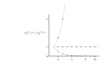
Figure 6.2: The maximum value for $\langle X_{0}\rangle^{2}+\langle Y_{0}\rangle^{2}$ obtainable by entangled quantum states (dots), by separable quantum states (crosses) and by LHV models (squares), plotted as a function of the number of qubits $N$. Note the exponential divergence between both the maxima obtained for entangled states as well as for separable states compared to the LHV value, where the former maximum is exponentially increasing and the latter maximum is exponentially decreasing.

6.4 Experimental strength of the $k$-separable
entanglement criteria

Violations of the above conditions for partial separability provide sufficient criteria for detecting $k$-separable entanglement (and $m$-partite entanglement with $\lceil N/k\rfloor\leq m\leq N-k+1$). It has already been shown that these criteria are stronger than the Laskowski-Żukowski criterion for $k$-inseparability for $k=2,N$ (i.e., detecting some and full entanglement), the fidelity criterion for full inseparability (i.e., full entanglement) and the Dür-Cirac criterion for inseparability under splits. In this section we will elaborate further on the experimental usefulness and strength of these entanglement criteria, when focusing on specific $N$-qubit states. The strength of an entanglement criterion to detect a given entangled state may be assessed by determining how well it copes with two desiderata tothguhne2: the noise robustness of the criterion for this given state should be high, and the number of local measurements settings needed for its implementation should be small.

In this section we will first take a closer look at the issue of noise robustness and at the number of required settings for implementation of the separability criteria, both in the general state-independent case and in the case of detecting target states. We then show the strength of the criteria for a variety of specific $N$-qubit states.

6.4.1 Noise robustness and the number of measurement
settings

White noise robustness of an entanglement criterion for a given entangled state is the maximal fraction $p_{0}$ of white noise which may be admixed to this state so that the state can no longer be detected as entangled by the criterion. Thus, for a given entangled state $\rho$, the noise robustness of a criterion is the threshold value $p_{0}$ for which the state $\rho=p\,\mathds{1}/2^{N}+(1-p)\rho$, with $p\geq p_{0}$ can no longer be detected by that criterion.

So, for the criterion for detecting full entanglement (6.105), the white noise robustness is found by solving the threshold equation for $p_{0}$:

$$|(1-p_{0})\rho_{l,\bar{l}}|=\sum_{j\neq l}\sqrt{(\frac{p_{0}}{2^{N}}+(1-p_{0})\rho_{j,j})(\frac{p_{0}}{2^{N}}+(1-p_{0})\rho_{\bar{\jmath},\bar{\jmath}})},$$ (6.111)

The state is fully entangled for $p<p_{0}$.

For the criterion (6.106), for detecting some entanglement, one finds a similar threshold equation:

$$\max_{l}\{|(1-p_{0})\rho_{l,\bar{l}}|^{2}\}=\min_{j}\{(\frac{p_{0}}{2^{N}}+(1-p_{0})\rho_{j,j})(\frac{p_{0}}{2^{N}}+(1-p_{0})\rho_{\bar{\jmath},\bar{\jmath}})\}.$$ (6.112)

This equation is quadratic and easily solved. Again, the state is entangled for $p<p_{0}$.

A local measurement setting setting; terhalComputSci; guhnehyllus is an observable such as $\mathcal{M}=\sigma_{1}\otimes\sigma_{l}\ldots\otimes\sigma_{N}$, where $\sigma_{l}$ denote single qubit observables for each of the $N$ qubits. Measuring such a setting (determining all coincidence probabilities of the $2^{N}$ outcomes) also enables one to determine the probabilities for observables like $\mathds{1}\otimes\sigma_{2}\ldots\otimes\sigma_{N}$, etc. guhne2007. Now consider the observables $X_{x}^{(N)}$ and $Y_{x}^{(N)}$ that appear in the separability criteria of (6.70)-(6.87). As is easily seen from their definitions in (6.69), one can measure such an observable using $2^{N}$ local settings. However, these same $2^{N}$ settings then suffice to measure the observables $X_{x}^{(N)}$ and $Y_{x}^{(N)}$ for all other $x$ since these are linear combinations of the same settings. Thus, $2^{N}$ measurement settings are sufficient to determine $\langle{X}_{x}^{(N)}\rangle$ and $\langle{Y}_{x}^{(N)}\rangle$ for all $x$. It remains to determine the number of settings needed for the terms $\langle I_{x}^{(N)}\rangle$ and $\langle Z_{x}^{(N)}\rangle$. For all $x$ these terms contain only two single-qubit observables: $Z^{(1)}$ and $I^{(1)}=\mathds{1}$. They can thus be measured by a single setting, i.e., $\left(Z^{(1)}\right)^{\otimes N}$.

Thus, in total $2^{N}+1$ settings are needed in order to test the separability conditions. This number grows exponentially with the number of qubits. However, this is the price we pay for being so general, i.e., for having criteria that work for all states. If we apply the criteria to detecting forms of inseparability and entanglement of specific entangled $N$-qubit states, this number can be greatly reduced. Knowledge of the target state enables one to select a single separability inequality for an optimal value of $x$ in (6.70)-(6.87). Violation of this single inequality is then sufficient for detecting the entanglement in this state, and, as we will now show, the required number of settings then grows only linear in $N$, with $N+1$ being the optimum for many states of interest.

For simplicity, assume that the local observables featuring in the criteria are the Pauli spin observables with the same orientation for each qubit. We can then readily use the density matrix representations of the separability criteria given at the end of each subsection in the previous section. Choosing the local observables differently amounts to performing suitable bases changes to the density matrix representations and would not affect the argument.

The matrix representations of the conditions show that only some anti-diagonal matrix elements and the values of some diagonal matrix elements have to be determined in order to test whether these inequalities are violated. Indeed, observe that for all $x$  $\langle I_{x}^{(N)}\rangle^{2}-\langle Z_{x}^{(N)}\rangle^{2}=4\rho_{j,j}\rho_{\bar{\jmath},\bar{\jmath}}$ with $\bar{\jmath}=d+1-j$ for some $j\in\{1,2,\ldots,d\}$ and $\langle X_{x}^{(N)}\rangle^{2}-\langle Y_{x}^{(N)}\rangle^{2}=4|\rho_{j,\bar{\jmath}}|^{2}$ denotes some anti-diagonal matrix element. It suffices to consider $x=0$ since conditions for other values of $x$ are obtained by some local unitary basis changes that will be explicitly given later on. We now want to rewrite the density matrix representation for this single separability inequality with $x=0$ in terms of less than $2^{N}+1$ settings.

Determining the diagonal matrix elements requires only a single setting, namely $\sigma_{z}^{\otimes N}$. Next, we should determine the modulus of the far-off anti-diagonal element $\rho_{1,d}$ ($d=2^{N}$) by measuring $X_{0}^{(N)}$ and $Y_{0}^{(N)}$, since $\langle X_{0}^{(N)}\rangle=2$Re$\rho_{1,d}$ and $\langle Y_{0}^{(N)}\rangle=2$Im$\rho_{1,d}$ (cf. (6.88)). Following the method of guhne2007, these matrix elements can be obtained from two settings $\mathscr{M}_{l}$ and $\tilde{\mathscr{M}}_{l}$, given by

$$\mathscr{M}_{l} =\big{(}\cos(\frac{l\pi}{N})\sigma_{x}+\sin(\frac{l\pi}{N})\sigma_{y}\big{)}^{\otimes N},\leavevmode\nobreak\ \leavevmode\nobreak\ \leavevmode\nobreak\ l=1,2,\ldots,N\leavevmode\nobreak\ ,$$ (6.113)

$$\tilde{\mathscr{M}}_{l} =\big{(}\cos(\frac{l\pi+\pi/2}{N})\sigma_{x}+\sin(\frac{l\pi+\pi/2}{N})\sigma_{y}\big{)}^{\otimes N},\leavevmode\nobreak\ \leavevmode\nobreak\ \leavevmode\nobreak\ l=1,2,\ldots,N.$$ (6.114)

These operators obey:

$$\sum_{l=1}^{N}(-1)^{l}\,\mathscr{M}_{l} =N\,X_{0}^{(N)},$$ (6.115)

$$\sum_{l=1}^{N}(-1)^{l}\,\tilde{\mathscr{M}}_{l} =N\,Y_{0}^{(N)}.$$ (6.116)

The proof of (6.115) is given by guhne2007 and (6.116) can be proven in the same way.

These relations show that the imaginary and the real part of an anti-diagonal element can be determined by the $N$ settings $\mathscr{M}_{l}$ and $\tilde{\mathscr{M}}_{l}$ respectively. This implies that the bi-separability condition (6.105) needs only $2N+1$ measurement settings. However, if each anti-diagonal term is real valued (which is often the case for states of interest) it can be determined by the $N$ settings $\mathscr{M}_{l}$, so that in total $N+1$ settings suffice.

Implementation of the criteria for other $x$ involves determining the modulus of some other anti-diagonal matrix element instead of the far-off anti-diagonal element $\rho_{1,d}$. The settings that allow for this determination can be obtained from a local unitary rotation on the settings $\mathscr{M}_{l}$ and $\tilde{\mathscr{M}}_{l}$ needed to measure $|\rho_{1,d}|$. This can be done as follows.

Suppose we want to determine the modulus of the matrix element $\rho_{j,\bar{\jmath}}$. The unitary rotation to be applied is given by $U_{j}=\sigma_{j_{1}}\otimes\sigma_{j_{2}}\otimes\ldots\otimes\sigma_{j_{N}}$ with $j=j_{1}j_{2}\ldots j_{N}$ in binary notation, with $\sigma_{0}=\mathds{1}$ and $\sigma_{1}=\sigma_{x}$. The settings that suffice are then given by $\mathscr{M}_{j,l}=U_{j}\,\mathscr{M}_{l}\,U_{j}^{\dagger}$ and $\tilde{\mathscr{M}}_{j,l}=U_{j}\,\tilde{\mathscr{M}}_{l}\,U_{j}^{\dagger}$ ($l=1,2,\ldots,N$). For example, take $N=4$ and suppose we want to determine $\rho_{5,4}$. We obtain the required settings by applying the local unitary $U_{5}=\mathds{1}\otimes\sigma_{x}\otimes\mathds{1}\otimes\sigma_{x}$ (since the binary notation of $5$ on four bits is $0101$) to the two settings $\mathscr{M}_{l}$ and $\tilde{\mathscr{M}_{l}}$ given in (6.113) and (6.116) respectively that for $N=4$ allow for determining $|\rho_{1,16}|$. In conclusion, using the above procedure the modulus of each anti-diagonal element can be determined using $2N$ settings, and in case they are real (or imaginary) $N$ settings suffice.

Since the strongest separability inequality for the specific target state under consideration is chosen, this reduction in the number of settings does not reduce the noise robustness for detecting forms of entanglement as compared to that obtained using the entanglement criteria in terms of the usual settings $X_{x}^{(N)}$, etc.

In conclusion, if the state to be detected is known, the $2N$ settings of (6.113) and (6.114) together with the single setting $\sigma_{z}^{\otimes N}$ suffice, and in case this state has solely real or imaginary anti-diagonal matrix elements only $N+1$ settings are needed. The white noise robustness using these settings is just as great as using the general condition that use the observables $X_{x}^{(N)}$ and $Y_{x}^{(N)}$, and is found by solving (6.111) or (6.112) for detecting full and some entanglement respectively.

As a final note, we observe that in order to determine the modulus of not just one but of all anti-diagonal matrix elements it is more efficient to use the observables $X_{x}^{(N)}$, $Y_{x}^{(N)}$ than the observables of (6.113) and (6.114). The first method needs $2^{N}$ settings to do this and the second needs $2^{N}N/2$ settings (since there are $2^{N}/2$ independent anti-diagonal elements), i.e., the latter needs more settings than the former for all $N$.

Let us apply the above procedure to an example, taken from guhne2007, the so-called four-qubit singlet state, which is given by:

$$|\,\Phi_{4}\rangle=(|\,0011\rangle+|\,1100\rangle-\frac{1}{2}(|\,01\rangle+|\,10\rangle)\otimes(|\,01\rangle+|\,10\rangle))/\sqrt{3}.$$ (6.117)

For detecting it as fully entangled (6.111) gives a noise robustness $p_{0}=12/29\approx 0.41$, and for detecting it as entangled (6.112) gives a noise robustness of $16/19\approx 0.84$. The implementation needs $16+1=17$ settings.

This number of settings can be reduced by using the fact that this state has only real anti-diagonal matrix elements and that we need only look at the largest anti-diagonal element. As shown above, this matrix element can be measured in $4$ settings. Thus the total number of settings required is reduced to only $5$. The off-diagonal matrix element to be determined is $|\,0011\rangle\langle\,1100|$. The four settings that allow for this determination are obtained from the four settings given in (6.113) by applying the unitary operator $U_{3}=\mathds{1}\otimes\mathds{1}\otimes\sigma_{x}\otimes\sigma_{x}$ to these settings.

For comparison, note that guhne2007 showed that the projector-based witness for the state (6.117) detects full entanglement with a white noise robustness $p_{0}=0.267$ and uses $15$ settings, whereas the optimal witness from guhne2007 uses only $3$ settings and has $p_{0}=0.317$. Here we obtain $p_{0}\approx 0.41$ using $5$ settings, implying a significant increase in white noise robustness using only two settings more.

This example gives the largest noise robustness when the conditions are measured in the standard $z$-basis. However, sometimes one obtains larger noise robustness when the state is first rotated so as to be expressed in a different basis before it is analyzed. For example, consider the four qubit Dicke state $|\,2,4\rangle$, where $|\,l,N\rangle=\binom{N}{l}^{-1/2}\sum_{k}\pi_{k}(|\,1_{1},\ldots,1_{l},0_{l+1},\ldots,0_{N}\rangle)$ are the symmetric Dicke states dicke (with $\{\pi_{k}(\cdot)\}$ the set of all distinct permutations of the $N$ qubits). In the standard basis this state does not violate any of the separability conditions we have discussed above. However, if each qubit is rotated around the $x$-axis by $90$ degrees all of the separability conditions can be violated with quite high noise robustness. Indeed, it is detected as inseparable under all splits through violation of conditions (6.75) for $p<p_{0}=16/19\approx 0.84$ and as fully entangled through violation of condition (6.77) for $p<p_{0}=4/11\approx 0.36$ using $5$ settings. For comparison, chen used specially constructed entanglement witnesses for detection of full entanglement in these states, and they obtained as noise robustness $p_{0}=2/9\approx 0.22$ using only $2$ settings. We have not performed an optimization procedure, so it is unclear whether or not the values obtained for $p_{0}$ can be improved.

6.4.2 Noise and decoherence robustness for the $N$-qubit GHZ state

In this subsection we determine the robustness of our separability criteria for detecting the $N$-qubit GHZ state in five kinds of noise processes (admixing white and colored noise, and three types of decoherence: depolarization, dephasing and dissipation of single qubits). We give the noise robustness as a function of $N$ for detecting some entanglement, inseparability with respect to all splits and full entanglement. We compare the results for white noise robustness of the criteria for full entanglement to that of the fidelity criterion (6.10) and to that of the so called stabilizer criteria of tothguhne2; tothguhne3.

The $N$-qubit GHZ state $|\,\Psi_{\mathrm{GHZ},0}^{N}\rangle=\frac{1}{\sqrt{2}}(|\,0\rangle^{\otimes N}+|\,1\rangle^{\otimes N}$) can be transformed into a mixed state $\rho_{N}$ by admixing noise to this state or by decoherence. Let us consider the following five such processes.

(i) Mixing in a fraction $p$ of white noise gives:

$$\rho_{N}^{\textrm{(i)}}=(1-p)|\,\Psi_{\mathrm{GHZ},0}^{N}\rangle\langle\,\Psi_{\mathrm{GHZ},0}^{N}|+p\frac{\mathds{1}}{2^{N}}.$$ (6.118)

(ii) Mixing in a fraction $p$ of colored noise noise2 gives:

$$\rho_{N}^{\textrm{(ii)}}=(1-p)|\,\Psi_{\mathrm{GHZ},0}^{N}\rangle\langle\,\Psi_{\mathrm{GHZ},0}^{N}|+\frac{p}{2}(|\,0\ldots 0\rangle\langle\,0\ldots 0|+|\,1\ldots 1\rangle\langle\,1\ldots 1|).$$ (6.119)

(iii) A depolarization process noise with a depolarization degree $p$ of a single qubit gives:

$$|\,i\rangle\langle\,j|\longrightarrow(1-p)|\,i\rangle\langle\,j|+p\,\delta_{ij}\frac{\mathds{1}}{2},$$

$$\rho_{N}^{\textrm{(iii)}}=\frac{1}{2}\big{[}\big{(}(1-\frac{p}{2})|\,0\rangle\langle\,0|+\frac{p}{2}|\,1\rangle\langle\,1|\big{)}^{\otimes N}+\big{(} \frac{p}{2}|\,0\rangle\langle\,0|+(1-\frac{p}{2})|\,1\rangle\langle\,1|\big{)}^{\otimes N}$$

$$+(1-p)^{N}\big{(}|\,0\rangle\langle\,1|^{\otimes N}+|\,1\rangle\langle\,0|^{\otimes N}\big{)}\big{]}.$$ (6.120)

(iv) A dephasing process noise with a dephasing degree $p$ of a single qubit gives:

$$|\,i\rangle\langle\,j|\longrightarrow(1-p)|\,i\rangle\langle\,j|+p\,\delta_{ij}|\,i\rangle\langle\,j|,$$

$$\rho_{N}^{\textrm{(iv)}}=\frac{1}{2}\big{[}|\,0\rangle\langle\,0|^{\otimes N}+|\,1\rangle\langle\,1|^{\otimes N}+(1-p)^{N}(|\,0\rangle\langle\,1|^{\otimes N}+|\,1\rangle\langle\,0|^{\otimes N})\big{]}.$$ (6.121)

(v) A dissipation process noise with a dissipation degree $p$ of a single qubit (where the ground state is taken to be $|\,0\rangle$) gives:

$$|\,i\rangle\langle\,i|\longrightarrow(1-p)|\,i\rangle\langle\,i|+p|\,0\rangle\langle\,0|,$$

$$|\,i\rangle\langle\,j|\longrightarrow(1-p)^{1/2}|\,i\rangle\langle\,j|,\leavevmode\nobreak\ \leavevmode\nobreak\ \leavevmode\nobreak\ \leavevmode\nobreak\ i\neq j,$$

$$\rho_{N}^{\textrm{(v)}}=\frac{1}{2}\big{[}|\,0\rangle\langle\,0|^{\otimes N}+(p|\,0\rangle\langle\,0|+(1-p)|\,1\rangle\langle\,1|)^{\otimes N}+$$

$$\leavevmode\nobreak\ \leavevmode\nobreak\ \leavevmode\nobreak\ \leavevmode\nobreak\ \leavevmode\nobreak\ \leavevmode\nobreak\ \leavevmode\nobreak\ \leavevmode\nobreak\ \leavevmode\nobreak\ \leavevmode\nobreak\ \leavevmode\nobreak\ \leavevmode\nobreak\ \leavevmode\nobreak\ \leavevmode\nobreak\ \leavevmode\nobreak\ \leavevmode\nobreak\ \leavevmode\nobreak\ \leavevmode\nobreak\ \leavevmode\nobreak\ \leavevmode\nobreak\ \leavevmode\nobreak\ \leavevmode\nobreak\ \leavevmode\nobreak\ \leavevmode\nobreak\ \leavevmode\nobreak\ \leavevmode\nobreak\ \leavevmode\nobreak\ \leavevmode\nobreak\ \leavevmode\nobreak\ \leavevmode\nobreak\ \leavevmode\nobreak\ \leavevmode\nobreak\ \leavevmode\nobreak\ \leavevmode\nobreak\ \leavevmode\nobreak\ \leavevmode\nobreak\ \leavevmode\nobreak\ \leavevmode\nobreak\ \leavevmode\nobreak\ \leavevmode\nobreak\ \leavevmode\nobreak\ \leavevmode\nobreak\ \leavevmode\nobreak\ \leavevmode\nobreak\ (1-p)^{N/2}(|\,0\rangle\langle\,1|^{\otimes N}+|\,1\rangle\langle\,0|^{\otimes N})\big{]}.$$ (6.122)

We now consider the question for what values of $p$ these states $\rho_{N}^{(\textrm{i})}$ to $\rho_{N}^{(\textrm{v})}$ are detected, firstly, as containing some entanglement (using the condition (6.106)) and, secondly, as inseparable under any split (using the conditions of the form (6.75) for all bi-partite splits). In other words, we determine the noise (or decoherence) robustness of violations of all these conditions for $\rho_{N}^{(\textrm{i})}$ to $\rho_{N}^{(\textrm{v})}$. We find the following threshold values $p_{0}$.

(i) $$p_{0}=\frac{1}{1+2^{(1-N)}},$$

(ii) $$p_{0}=1,\leavevmode\nobreak\ \leavevmode\nobreak\ \leavevmode\nobreak\ \leavevmode\nobreak\ \forall N,$$

(iii) $$(1-p_{0})^{N}=(1-\frac{p_{0}}{2})^{\alpha}(\frac{p_{0}}{2})^{(N-\alpha)}+(1-\frac{p_{0}}{2})^{(N-\alpha)}(\frac{p_{0}}{2})^{\alpha},$$ (6.123)

(iv) $$p_{0}=1,\leavevmode\nobreak\ \leavevmode\nobreak\ \leavevmode\nobreak\ \leavevmode\nobreak\ \forall N,$$

(v) $$p_{0}=1,\leavevmode\nobreak\ \leavevmode\nobreak\ \leavevmode\nobreak\ \leavevmode\nobreak\ \forall N.$$

For cases (i), (ii), (iv) and (v) the threshold values $p_{0}$ for detecting some entanglement and inseparability with respect to all splits are the same because for these cases the product of the diagonal matrix elements $\rho_{j,j}\rho_{\bar{j},\bar{j}}$ is the same for all $j\neq 1,d$. Only in case (iii) is this product different for different $j$. We then have to take the minimum and maximum value, respectively, from which it follows that $\alpha$ is to be set to $[N/2]$ for detecting some entanglement and to $1$ for detecting inseparability with respect to all splits. Here $[N/2]$ is the largest integer smaller or equal to $N/2$.

The result in case (i) is in accordance with the results of duer2; duer, where it is furthermore shown that the opposite holds as well, i.e., iff $p<1/(1+2^{(1-N)})$ then $\rho_{N}^{\textrm{(i)}}$ is inseparable under any split and otherwise it is fully separable. Thus all states of the form (6.118) that are inseparable under any split are detected by violations of the conditions of the form (6.75) for all bi-partite splits. The same holds for cases (ii), (iv) and (v), since all states $\rho_{N}^{\textrm{(ii)}}$, $\rho_{N}^{\textrm{(iv)}}$ and $\rho_{N}^{\textrm{(v)}}$ are inseparable under any split for all $p<1$. In other words, as soon as a fraction of the GHZ state is present, these states are inseparable under any split. In case (i) $p_{0}$ increases monotonically from $p_{0}=2/3$ for $N=2$ to $p_{0}=1$ for large $N$. For process (iii) these limiting values are not so straightforward: $p_{0}=(3-\sqrt{3})/3\approx 0.42$ for $N=2$, and $p_{0}=(5-\sqrt{5})/5\approx 0.55$ for large $N$. In conclusion, the noise and decoherence robustness is high for all $N$, except maybe for case (iii).

Next, consider the noise robustness for detecting full entanglement by means of the bi-separability condition (6.77). The result is the following:

(i) $$p_{0}=1/(2(1-2^{-N})),$$

(ii) $$p_{0}=1,\leavevmode\nobreak\ \leavevmode\nobreak\ \leavevmode\nobreak\ \leavevmode\nobreak\ \forall N,$$

(iii) $$p_{0}\approx 0.42,0.28,0.22,0.18,\leavevmode\nobreak\ \leavevmode\nobreak\ N=2,3,4,5.$$ (6.124)

(iv) $$p_{0}=1,\leavevmode\nobreak\ \leavevmode\nobreak\ \leavevmode\nobreak\ \leavevmode\nobreak\ \forall N,$$

(v) $$p_{0}\approx 1,0.48,0.39,0.35,\leavevmode\nobreak\ \leavevmode\nobreak\ N=2,3,4,5.$$

For case (i) the noise robustness is equivalent to the fidelity criterion (6.10). For large $N$ $p_{0}$ decreases to the limit value $p_{0}=1/2$. Case (ii) and (iv) have $p_{0}=1$, thus as soon as the states $\rho_{N}^{\textrm{(ii)}}$ and $\rho_{N}^{\textrm{(iv)}}$ are entangled they are fully entangled. For cases (iii) and (v) we listed the noise robustness found numerically for $N=2$ to $N=5$. These values decrease for increasing $N$.

Let us compare the results for white noise robustness (case (i)) to the results obtained from the so-called stabilizer formalism gottesman. This formalism is used by tothguhne2; tothguhne3 to derive entanglement witnesses that are especially useful for minimizing the number of settings required to detect either full or some entanglement. Here we will only consider the criteria formulated for detecting entanglement of the $N$-qubit GHZ states. The stabilizer witness by Tóth & Gühne that detects some entanglement has $p_{0}=2/3$, independent of $N$, and requires only three settings (cf.  Eq. (13) in tothguhne2). The strongest witness for full entanglement of Tóth & Gühne has a robustness $p_{0}=1/(3-2^{(2-N)})$ and requires only two settings (cf. Eq. (23) in tothguhne2).

Figure 6.3 shows these threshold noise ratios for detecting full entanglement for these three criteria. Note that the criterion of tothguhne2 needs only two measurement settings, whereas our criteria need $N+1$ settings. So although the former are less robust against white noise admixture, they compare favorably with respect to minimizing the number of measurement settings.

Although we give a criterion for full entanglement that is generally stronger than the fidelity criterion, for the $N$-partite GHZ state this does not lead to better noise robustness. It appears that for large $N$ the noise threshold $p_{0}=1/2$ is the best one can do. However, in the limit of large $N$ the GHZ state is inseparable under all splits for all $p_{0}<1$, as was shown in (i) in (6.4.2). See also Figure 6.3.

We have seen that if the state $\rho_{N}^{\textrm{(i)}}$ is entangled it is also inseparable under any split. Because of the high symmetry of both the GHZ state and white noise, one might conjecture that if this state is entangled it is also fully entangled. At present, however it is unknown whether this is indeed true. Detecting the states $\rho_{N}^{\textrm{(i)}}$ as fully entangled appears to be a much more demanding task than detecting them as inseparable under all splits. In the first case, for large $N$, only a fraction of $50\%$ noise is permitted, in the second case one can permit any noise fraction (less than $100\%$). Note that we have given explicit examples of states that are diagonal in the GHZ basis (cf. (6.14) of section 6.2.2), and that are inseparable under any split, but not fully entangled. But these are not of the form $\rho_{N}^{\textrm{(i)}}$.

Lastly, we mention that our criteria detect the various forms of entanglement and inseparability also if the state $|\,\Psi_{\mathrm{GHZ},0}^{N}\rangle$ is replaced by any other maximally entangled state (i.e., any state of the GHZ basis, cf. (6.13)), a feature which is not possible using linear entanglement witnesses. There is no single linear witness that detects entanglement of all maximally entangled states.

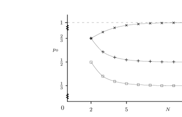
Figure 6.3: The threshold noise ratios $p_{0}$ for detection of full $N$-qubit entanglement when admixing white noise to the $N$-qubit GHZ state for the criterion (6.77) derived here (plus-signs) and for the stabilizer witness of tothguhne2 (squares). The noise robustness for detecting inseparability under all splits as given in (i) in (6.4.2) is also plotted (crosses).

6.4.3 Detecting bound entanglement for $N\geq 3$

Violation of the separability inequality (6.85) allows for detecting all bound entangled states of dur. These states have the form

$$\rho_{B}=\frac{1}{N+1}\left(|\,\Psi_{{\rm GHZ},\alpha}^{N}\rangle\langle\,\Psi_{{\rm GHZ},\alpha}^{N}|+\frac{1}{2}\sum_{l=1}^{N}P_{l}+\bar{P}_{l}\right),$$ (6.125)

with $P_{l}$ the projector on the state $|\,0\rangle_{1}\ldots|\,1\rangle_{l}\ldots|\,0\rangle_{N}$, and where $\bar{P}_{l}$ is obtained from $P_{l}$ by replacing all zeros by ones and vice versa. For $N\geq 4$ these states are entangled and have positive partial transposition (PPT) with respect to transposition of any qubit. This means they are bound entangled bound. Note that they are detected as entangled by the $N$-partite Mermin inequality $|M_{N}|\leq 2$ of section 6.3.3 only for $N\geq 8$ dur. However, the condition (6.85) detects them as entangled for $N\geq 4$. Thus all bound entangled states of this form are detected as entangled by this latter condition. The white noise robustness for this purpose is $p_{0}=2^{N}/(2+2N+2^{N})$, which for $N=4$ gives $p_{0}=8/13\approx 0.615$ and goes to $1$ for large $N$. Note that for $N=4$, this state violates the condition for $4$-separability, and the condition for $3$-separability (6.87), but not the condition for $2$-separability. It is thus at least $2$-separable entangled. It is not detected as fully entangled by these criteria. (Of course, it could still be fully entangled since these criteria are only sufficient and not necessary for entanglement). For general $N$ we have not investigated the $k$-separable entanglement of the states (6.125), although this can be readily performed using the criteria of (6.87).

Another interesting bound entangled state is the so-called four qubit Smolin state smolin

$$\rho_{S}=\frac{1}{4}\sum_{j=1}^{4}|\,\Psi^{j}_{ab}\rangle\langle\,\Psi^{j}_{ab}|\otimes|\,\Psi^{j}_{cd}\rangle\langle\,\Psi^{j}_{cd}|,$$ (6.126)

where $\{|\,\Psi^{j}\rangle\}$ is the set of four Bell states $\{|\,\phi^{\pm}\rangle,|\,\psi^{\pm}\rangle\}$, and $a,b,c,d$ label the four qubits. This state is also detected as entangled by the criterion (6.85), and with white noise robustness $p_{0}=2/3$. The Smolin state violates the separability conditions (6.75) for bi-separability under the splits $a$-$(bcd)$, $b$-$(acd)$, $c$-$(abd)$, $d$-$(abc)$. However, it is separable under the splits $(ab)$-$(cd)$, $(ac)$-$(bd)$, $(ad)$-$(bc)$ (cf. smolin). This state is thus inseparable under splits that partition the system into two subsets with one and three qubits, but it is separable when each subset contains two qubits.

So far we have detected bound entanglement for $N\geq 4$. What about $N=3$? Consider the three-qubit bound entangled state of duer22:

$$\rho=\frac{1}{3}|\,\Psi_{GHZ,0}^{3}\rangle\langle\,\Psi_{GHZ,0}^{3}|+\hskip-0.71114pt\frac{1}{6}(|\,001\rangle\langle\,001|+\hskip-0.71114pt|\,010\rangle\langle\,010|+\hskip-0.71114pt|\,101\rangle\langle\,101|+\hskip-0.71114pt|\,110\rangle\langle\,110|).$$ (6.127)

This state is detected as entangled by the criterion (6.44), with white noise robustness $p_{0}=4/7\approx 0.57$. It violates the bi-separability condition (6.33) for the split $a$-$(bc)$ so it is at least bi-separable entangled, but does not violate the condition (6.43) for bi-separability i.e., it is not detected as fully entangled. In fact, it can be shown using the results of duer that this state is separable under the splits $b$-$(ac)$ and $c$-$(ab)$.

6.5 Discussion

We have discussed partial separability of quantum states by distinguishing $k$-separa-bility from $\alpha_{k}$-separability and used these distinctions to extend the classification proposed by Dür and Cirac. We discussed the relationship of partial separability to multi-partite entanglement and distinguished the notions of a $k$-separable entangled state and a $m$-partite entangled state and indicated the interrelations of these kinds of entanglement.

Next, we have presented necessary conditions for partial separability in the hierarchic separability classification. These are formulated in terms of experimentally accessible correlation inequalities for operators defined by products of local orthogonal observables. Violations of these inequalities provide, for all $N$-qubit states, criteria for the entire hierarchy of $k$-separable entanglement, ranging from the levels $k$=1 (full or genuine $N$-particle entanglement) to $k=N$ (full separability, no entanglement), as well as for specific classes within each level. Choosing the Pauli matrices as the locally orthogonal observables provided matrix representations of the criteria that bound anti-diagonal matrix elements in terms of diagonal ones.

Further, the $N$-qubit Mermin-type separability inequalities for partial separability were shown to follow from the partial separability conditions derived in this chapter. The bi-separability conditions are stronger than the fidelity criterion and the Laskowski-Żukowski criterion, and the latter criterion is also shown to be strengthened for full separability and biseparability. For separability under splits the conditions are stronger than the Dür-Cirac conditions. Violation of these conditions thus give entanglement criteria that detect more entangled states than violations of these three other separability conditions.

We have furthermore shown that the required number of measurement settings for implementation of these criteria, which is $2^{N}+1$ in general, can be drastically reduced if entanglement of a given target state is to be detected. In that case, it may be reduced to $2N+1$, and for multi-qubit states with either real or imaginary anti-diagonal matrix elements, only $N+1$ settings are needed.

When comparing the entanglement criteria to other state-specific multi-qubit entanglement criteria it was found that the white noise robustness was high for a great variety of interesting multi-qubit states, whereas the number of required settings was only $N+1$. However, these other state-specific entanglement criteria need less settings although for the states analyzed here they give lower noise robustness. Analyzing some specific target states shows that the entanglement criteria detect bound entanglement for $N\geq 3$.

Furthermore, we applied the entanglement criteria for some and full entanglement to the $N$-qubit GHZ state subjected to two different kinds of noise and three different kinds of decoherence. The robustness against colored noise and against dephasing turns out to be maximal (i.e., $p_{0}=1$) both for detecting some and full entanglement. It is remarkable that for large $N$ the GHZ state allows for maximal white noise robustness for the state to remain inseparable under all possible splits, whereas for detecting full entanglement the best known result – to our best knowledge – only allows for a white noise robustness of $p_{0}=1/2$. It would be very interesting to search for full entanglement criteria that can close this gap, or if this is shown to be impossible to understand why this is the case.

Orthogonality of the local observables is crucial in the above derivation of separability conditions. It is due to this assumption that the multi-qubit operators form representations of the generalized Pauli group. It would be interesting to analyze the role of orthogonality in deriving the inequalities. For two qubits it has been shown by tradeoff, see chapter 5, that when orthogonality is relaxed the separability conditions become less strong, and we conjecture the same holds for their multi-qubit analogs. Relaxing the requirement of orthogonality has the advantage that some uncertainty in the angles may be accommodated, which is desirable since in real experiments it may be hard to measure perfectly orthogonal observables.

It is also interesting that the separability inequalities are equivalent to bounds on anti-diagonal matrix elements in terms of products of diagonal ones. We thus gain a new perspective on why they allow for entanglement detection: they probe the values of anti-diagonal matrix elements, which encode entanglement information about the state; and if these elements are large enough, this entanglement is detected. Note furthermore that compared to the Mermin-type separability inequalities we need not do much more to obtain our stronger inequalities. We must solely determine some diagonal matrix elements, and this can be easily performed using the single extra setting $\sigma_{z}^{\otimes N}$.

Our recursive definition of the multi-partite correlation operators (see (6.69)) is by no means unique. One can generate many new inequalities by choosing the locally orthogonal observables differently, e.g., by permuting their order in each triple of local observables. It could well be that combining such new inequalities with those presented here yield even stronger separability conditions, as is indeed the case for pure two-qubit states uffseev, see chapter 4. Unfortunately, we have no conclusive answers for this open question.

We end by suggesting three further lines of future research. Firstly, it would be interesting to apply the entanglement criteria to an even larger variety of $N$-qubit states than analyzed here, including for example all $N$-qubit graph and Dicke states. Secondly, the generalization from qubits to qudits (i.e., $d$-dimensional quantum systems) would, if indeed possible, prove very useful since strong partial separability criteria for $N$ qudits have – to our knowledge – not yet been obtained. And finally, it would be beneficial to have optimization procedures for choosing the set of local orthogonal observables featuring in the entanglement criteria that gives the highest noise robustness for a given set of states. We believe we have chosen such optimal sets for the variety of states analyzed here, but since no rigorous optimization was performed, our choices could perhaps be improved.

To end this chapter we comment on the noteworthy result that the Mermin-type separability inequalities show that the strength of the correlations in separable qubit states is exponentially decreasing when compared to the strength of the correlations allowed for by LHV models. From a more fundamental point of view it is quite remarkable that the strengthened Bell-type inequalities which were shown to hold for separable qubit states, do not hold for LHV theories, for which the Bell-type inequalities were originally designed. This shows that the latter theories are able to give correlations for which quantum mechanics, in order to reproduce them using qubit states, needs recourse to entangled states; and even more and more so when the number of particles increases.

Assuming that the LHV doctrine is a necessary ingredient for the notion of classicality, the idea that it is the separable qubit states which are the classical states among all qubit states needs revision. Although werner was the first to point to this, we here show a much more radical and general departure, especially when the number of qubits grows. Of course, if more general measurement scenarios than the standard Bell experiment setup are allowed things might change. Given the surprising results found here between separability of qubit states and local hidden-variable structures, the question what is exactly the classical part of quantum mechanics seems to still be not fully answered and open for new investigations.

However, it should be mentioned that, just as was the case in chapter 4 for the two-qubit separability inequalities, these findings hold only for the case of qubits. By choosing the Hilbert space of the systems under consideration to be large enough any choice of observables can be made commuting. Using separable states of a system consisting of such systems one can, after all, reproduce the predictions of all LHV models.

Thus one may take an experimental violation of the Mermin-type separability inequalities by $N$-qubits to mean two things: (i) either one can conclude that the state of the $N$-qubits is entangled, or (ii) the state might be separable but then one is not dealing with qubits after all and some degrees of freedom must have been overlooked.

Chapter 7 Monogamy of correlations

This chapter is in part based on seevmon.

7.1 Introduction to the monogamy of entanglement
and of correlations

If a pure quantum state of two systems is entangled, then none of the two systems can be entangled with a third system. This can be easily seen. Suppose that systems $a$ and $b$ are in a pure entangled state. Then when the system $ab$ is considered as part of a larger system, the reduced density operator for $ab$ must by assumption be a pure state. However, for the composite system $ab$ (or for any of its subsystems $a$ or $b$) to be entangled with another system, the reduced density operator of $ab$ must be a mixed state. But since it is by assumption pure, no entanglement between $ab$ and any other system can exist. This feature is referred to as the monogamy of pure state entanglement.

This monogamy can also be understood as a consequence of the linearity of quantum mechanics that is also responsible for the no-cloning theorem. For suppose that party $a$ has a qubit which is maximally pure state entangled to both a qubit held by party $b$ and a qubit held by party $c$. Party $a$ thus has a single qubit coupled to two perfect entangled quantum channels, which this party could exploit to teleport two perfect copies of an unknown input state, thereby violating the no-cloning theorem, and thus the linearity of quantum mechanics terhal.

If the state of two systems is not a pure entangled state but a mixed entangled state, then it is possible that both of the two systems are entangled to a third system. For example, the $W$-state $|\,\psi\rangle=(|\,001\rangle+|\,010\rangle+|\,100\rangle)/\sqrt{3}$ has bi-partite reduced states that are all identical and entangled. This feature is called ‘sharing of mixed state entanglement’, or ‘promiscuity of entanglement’. So we see that entanglement is strictly speaking only monogamous in the case of pure entangled states. In the case of mixed entangled states it can be promiscuous. But this promiscuity is not unbounded: although some entangled bi-partite states may be shareable with some finite number of parties, no entangled bi-partite state can be shared with an infinite number of parties. Here a bi-partite state $\rho_{ab}$ is said to be $N$-shareable when it is possible to find a quantum state $\rho_{a{b_{1}}{b_{2}}\ldots{b_{N}}}$ such that $\rho_{ab}=\rho_{{a{b_{1}}}}=\rho_{a{b_{2}}}=\ldots=\rho_{a{b_{N}}}$, where $\rho_{a{b_{k}}}$ is the reduced state for parties $a$ and $b_{k}$. Consider the following theorem fannes; raggio: A bi-partite state is $N$-shareable for all $N$ (also called $\infty$-shareable masanes06) iff it is separable. Thus no bi-partite entangled state, pure or mixed, is $N$-shareable for all $N$.

The monogamy of entanglement was first quantified by ckw who gave a trade-off relation between how entangled $a$ is with $b$, and how entangled $a$ is with $c$ in a three-qubit system $abc$ that is in a pure state, using the measure of bi-partite entanglement called the tangle osborne. It states that $\tau(\rho_{ab})+\tau(\rho_{ac})\leq\tau(\rho_{a(bc)})$ where $\tau(\rho_{ab})$ is the tangle between $A$ and $B$, analogous for $\tau(\rho_{ac})$ and $\tau(\rho_{a(bc)})$ is the bi-partite entanglement across the split $a$-$(bc)$. The multi-partite generalization has been recently proven by osborne. In general, $\tau$ can vary between $0$ and $1$, but monogamy constrains the entanglement (as quantified by $\tau$) that party $a$ can have with each of parties $b$ and $c$.

Classically one does not have such a trade-off. All classical probability distributions can be shared toner2. If parties $a$, $b$ and $c$ have bits instead of quantum bits (qubits) and if $a$’s bit is always the same as $b$’s bit then there is no restriction on how $a$’s bit is correlated to $c$’s bit.

Let us however not just look at entanglement but also at correlations that result from making local measurements on quantum systems. As we have seen many times already, these correlations can violate Bell-type inequalities that hold for local hidden-variable models. Such Bell-type inequality violating correlations turn out to be monogamous. This is termed ‘monogamy of quantum non-locality’ or ‘non-local correlations are monogamous’.

Let us show this in a setup where each party implements two possible dichotomous observables. The CHSH inequality is the only non-trivial local Bell-type inequality for this setup. All quantum correlations that violate this inequality are monogamous as follows from the following tight trade-off inequality for a three-partite system $abc$ proven by tonerverstraete:

$$\langle\mathcal{B}_{ab}\rangle_{\textrm{qm}}^{2}+\langle\mathcal{B}_{ac}\rangle_{\textrm{qm}}^{2}\leq 8,$$ (7.1)

where $\mathcal{B}_{ab}$ is the CHSH operator (4.1) for parties $a$ and $b$, and analogous for $\mathcal{B}_{ac}$.

Figure 7.1: Monogamy of quantum and no-signaling correlations. All quantum correlations lie within the circle, and all no-signaling correlations lie within the tilted larger square. For comparison the classical correlations are also shown. These lie within the square with edge length $2$. The correlations obtainable by orthogonal measurements on separable two-qubit states lie within the smallest square.

Quantum correlations thus show an interesting trade-off relationship: In case the correlations between party $a$ and $b$ are non-local (i.e., when $|\langle\mathcal{B}_{ab}\rangle_{\textrm{qm}}|>2$) the correlations between parties $a$ and $c$ cannot be non-local (i.e., necessarily $|\langle\mathcal{B}_{ac}\rangle_{\textrm{qm}}|\leq 2$), and vice versa (cf. scarani). These non-local quantum correlations can thus not be shared. Furthermore, in case they are maximally non-local, i.e., $|\langle\mathcal{B}_{ab}\rangle_{\textrm{qm}}|=2\sqrt{2}$ the other must be uncorrelated, i.e., it must be that $|\langle\mathcal{B}_{ac}\rangle_{\textrm{qm}}|=0$, and vice versa. Here it is crucial that the measurements performed by party $a$ are the same in both expressions.

This trade-off relation is plotted in Figure 7.1. It provides a non-trivial bound on the set of quantum correlations because a three-partite system $abc$ cannot simultaneously violate the CHSH inequality for correlations between $ab$ (summing over $c$’s outcomes) and between $ac$ (summing over $c$’s outcomes). Both general unrestricted and local correlations do not obey such a monogamy trade-off. The first type can reach the absolute maxima $|\mathcal{B}_{ab}|_{\textrm{max}}=|\mathcal{B}_{ac}|_{\textrm{max}}=4$, and the second type can attain the maximal value for local correlations, i.e, $\langle\mathcal{B}_{ab}\rangle_{\textrm{lhv}}=\langle\mathcal{B}_{ac}\rangle_{\textrm{lhv}}=2$.

The reason for this is that general unrestricted correlations and local correlations can be shared. The latter fact is proven by masanes06 and the first we will prove here. However, first we need the relevant definitions. Shareability of a general unrestricted probability distribution is defined as follows (where for simplicity we restrict ourselves to shareability of bi-partite distributions). A bi-partite distribution $P(a,b_{1}|A,B_{1},\ldots,B_{N})$ is $N$-shareable with respect to the second party if an $(N+1)$-partite distribution $P(a,b_{1},\ldots,b_{N}|A,B_{1},\ldots,B_{N})$ exists that is symmetric with respect to $(b_{1},B_{1}),\,(b_{2},B_{2}),\,\ldots,\,(b_{N},B_{N})$ and with marginals $P(a,b_{i}|A,B_{1},\ldots,B_{N})$ equal to the original distribution $P(a,b_{1}|A,B_{1},\ldots,B_{N})$, for all $i$. For notational clarity we use $b_{i}$ and $B_{i}$ (instead of $a_{i}$ and $A_{i}$) to denote outcomes and observables respectively for the parties other than the first party. If a distribution is shareable for all $N$ it is called $\infty$-shareable.

Shareability of a no-signaling probability distribution is defined analogously: A no-signaling distribution $P(a,b_{1}|A,B_{1})$ is $N$-shareable with respect to the second party if there exist an $(N+1)$-partite distribution $P(a,b_{1},\ldots,b_{N}|A,B_{1},\ldots,B_{N})$ being symmetric with respect to $(b_{1},B_{1}),\,(b_{2},B_{2}),\,\ldots,\,(b_{N},B_{N})$ with marginals $P(a,b_{i}|A,B_{i})$ equal to the original distribution $P(a,b_{1}|A,B_{1})$, for all $i$. The difference between shareability of unrestricted correlations and of no-signaling correlations is that in the first case the marginals depend on all $N+1$ settings, whereas in the latter case they only depend on the two settings $A$ and $B_{i}$.

Suppose we are given a general unrestricted correlation $P(a,b_{1}|A,B_{1},\ldots,B_{N})$. We can then construct

$$P(a,b_{1},\ldots,b_{N}|A,B_{1},\ldots,B_{N})=P(a,b_{1}|A,B_{1},\ldots,B_{N})\delta_{b_{1},b_{2}}\cdots\delta_{b_{1},b_{N}},$$ (7.2)

which has by construction the same marginals $P(a,b_{i}|A,B_{1},\ldots,B_{N})$ equal to the original distribution $P(a,b_{1}|A,B_{1},\ldots,B_{N})$. This holds for all $i$, thereby proving the $\infty$-shareability. Thus an unrestricted correlation can be shared for all $N$. If we restrict the distributions to be no-signaling, masanes06 proved that $\infty$-shareability implies that the distribution is local, i.e., it can be written as

$$P(a,b_{1},\ldots,b_{N})|A,B_{1}\ldots,B_{N})=\int_{\Lambda}d\lambda p(\lambda)P(a|A,\lambda)P(b_{1}|B_{1},\lambda)\cdots P(b_{N}|B_{N},\lambda),$$ (7.3)

for some local distributions $P(a|A,\lambda),P(b_{1}|B_{1},\lambda),\ldots,P(b_{N}|B_{N},\lambda)$ and hidden-variable distribution $p(\lambda)$.

Because general unrestricted correlations and local ones can be shared they both will not show any monogamy. This implies that partially-local correlations also do not show any monogamy, since these are combinations of local and general unrestricted correlations between subsystems of the $N$-systems.

The above result by masanes06 shows that quantum and no-signaling correlations can not be $\infty$-shareable and they must therefore show monogamy effects. Monogamy of quantum correlations has already been shown above via the trade-off relation (7.1), so let us move to no-signaling correlations. First consider a very strong monogamy property for extremal no-signaling correlations, already mentioned by barrett05. Suppose one has some no-signaling three-party probability distribution $P(a_{1},a_{2},a_{3}|A_{1},A_{2},A_{3})$ for parties $a$, $b$ and $c$. In case the marginal distribution $P(a_{1},a_{2}|A_{1},A_{2})$ of system $ab$ is extremal then it cannot be correlated to the third system $c$, as the following proof by barrett05 shows.

Bayes’ rule and no-signaling give

$$P(a_{1},a_{2},a_{3}|A_{1},A_{2},A_{3}) =P(a_{1},a_{2},|A_{1},A_{2},A_{3},a_{3})P(a_{3}|A_{1},A_{2},A_{3})$$

$$=P(a_{1},a_{2}|A_{1},A_{2},A_{3},a_{3})P(a_{3}|A_{3}).$$ (7.4)

Therefore the marginal $P(a_{1},a_{2}|A_{1},A_{2})$ can be rewritten as

$$P(a_{1},a_{2}|A_{1},A_{2}) =\sum_{a_{3}}P(a_{1},a_{2},a_{3}|A_{1},A_{2},A_{3})$$

$$=\sum_{a_{3}}P(a_{1},a_{2}|A_{1},A_{2},A_{3},a_{3})P(a_{3}|A_{3}),\leavevmode\nobreak\ \forall A_{3}.$$ (7.5)

Since by supposition $P(a_{1},a_{2}|A_{1},A_{2})$ is extremal the decomposition is unique, this gives
$P(a_{1},a_{2}|A_{1},A_{2},A_{3},a_{3})=P(a_{1},a_{2}|A_{1},A_{2}),\forall a_{3},A_{3}$. Then combining all this gives:

$$P(a_{1},a_{2},a_{3}|A_{1},A_{2},A_{3})=P(a_{1},a_{2}|A_{1},A_{2})P(a_{3}|A_{3}),$$ (7.6)

which implies that party $c$ is completely uncorrelated with party $ab$: the extremal correlation $P(a_{1},a_{2}|A_{1},A_{2})$ is completely monogamous. Note that this implies that all local Bell-type inequalities for which the maximal violation consistent with no-signaling is attained by a unique correlation have monogamy constraints. This follows because all Bell-type inequalities are linear in the correlations, therefore, if the maximal violation is produced by a unique correlation, it can only be produced by an extreme point of the no-signaling polytope. Otherwise the correlation that produces maximal violation would not be unique. An example is the CHSH inequality, as will be shown below.

Extremal no-signaling correlations thus show monogamy, but what about non-extremal no-signaling correlations? Just as was the case for quantum states where non-extremal (mixed state) entanglement can be shared, non-extremal no-signaling correlations can be shared as well. This can be seen from the fact that no-signaling correlations obey the following tight trade-off relation in terms of the CHSH operators toner2:

$$|\langle\mathcal{B}_{ab}\rangle_{\textrm{ns}}|+|\langle\mathcal{B}_{ac}\rangle_{\textrm{ns}}|\leq 4.$$ (7.7)

This is also depicted in Figure 7.1. Extremal no-signaling correlations can attain $|\langle\mathcal{B}_{ab}\rangle_{\textrm{ns}}|=4$ so that necessarily $|\langle\mathcal{B}_{ac}\rangle_{\textrm{ns}}|=0$, and vice versa (this is monogamy of extremal no-signaling correlations), whereas non-extremal ones are shareable since the correlation terms $|\langle\mathcal{B}_{ab}\rangle_{\textrm{ns}}|$ and $|\langle\mathcal{B}_{ac}\rangle_{\textrm{ns}}|$ can both be non-zero at the same time. But note that in case the no-signaling correlations are non-local they can not be shared, i.e., it is not possible that $|\langle\mathcal{B}_{ab}\rangle_{\textrm{ns}}|\geq 2$ and $|\langle\mathcal{B}_{ac}\rangle_{\textrm{ns}}|\geq 2$. This shows that if these non-local correlations can be shared they must be signaling.

For general unrestricted correlations no monogamy holds, i.e., $|\langle\mathcal{B}_{ab}\rangle|$ and $|\langle\mathcal{B}_{ac}\rangle|$ are not mutually constrained and can each obtain a value of $4$ so as to give the absolute maximum of the left hand side of (7.7) which is the value $8$. The monogamy bound (7.7) therefore gives a way of discriminating no-signaling from general correlations: if it is violated the correlations cannot be no-signaling (i.e., they must be signaling). This discerning inequality uses product expectation values only, in contrast to the facets of the no-signaling polytope that only give non-trivial constrains on the marginal expectation values, as was discussed in chapter 2, section 2.3.1.1.

For classical correlations no such trade-off as in (7.1) or as in (7.7) holds. Indeed, it is possible to have both $|\langle\mathcal{B}_{ab}\rangle_{\textrm{lhv}}|=2$ and $|\langle\mathcal{B}_{ac}\rangle_{\textrm{lhv}}|=2$, see also Figure 7.1. This reflects the fact that classical correlations are always shareable. The correlations that separable quantum states allow for are also shareable. Indeed, in the $\langle\mathcal{B}_{ab}\rangle_{\textrm{qm}}$-$\langle\mathcal{B}_{ac}\rangle_{\textrm{qm}}$ plane of Figure 7.1 such correlations can reach the full square with edge length $2$. Analogous to what we have seen in chapter 5, it is the case that when considering qubits and measurements that are restricted to orthogonal ones only one obtains tighter bounds. These restrict the possible values of $\langle\mathcal{B}_{ab}\rangle_{\textrm{qm}}$ and $\langle\mathcal{B}_{ac}\rangle_{\textrm{qm}}$ to the smallest square of Figure 7.1: $|\langle\mathcal{B}_{ab}\rangle_{\textrm{qm}}|,|\langle\mathcal{B}_{ac}\rangle_{\textrm{qm}}|\leq\sqrt{2}$, $\rho\in\mathcal{D}_{\textrm{sep}}$. But again there is no monogamy for separable states in this case since this full square can be reached.

7.1.1 A stronger monogamy relation for the non-locality of
bi-partite quantum correlations

We will now give an alternative simpler proof of the inequality (7.1) that also allows us to strengthen it as well. The proof uses the idea that (7.1), which describes the interior of a circle in the $\langle\mathcal{B}_{ab}\rangle$-$\langle\mathcal{B}_{ac}\rangle$ plane, is equivalent to the interior of the set of tangents to this circle. It is thus a compact way of writing the following infinite set of linear equalities

$$\mathcal{S}=\max_{\theta}\langle\mathcal{S}_{\theta}\rangle_{\textrm{qm}}\leq 2\sqrt{2},$$ (7.8)

where we have used $\sqrt{x^{2}+y^{2}}=\max_{\theta}(\cos\theta\,x+\sin\theta\,y)$, and where $\mathcal{S}_{\theta}=\cos\theta\,\mathcal{B}_{ab}+\sin\theta\,\mathcal{B}_{ac}$.

We will now prove this by showing that $|\langle\mathcal{B}_{ab}\cos\theta+\mathcal{B}_{ac}\sin\theta\rangle_{\textrm{qm}}|\leq 2\sqrt{2}$ for all $\theta$, using a method presented by dieks in a different context. In this proof we only consider quantum correlations so for brevity we drop the subscript ‘qm’ from the expectation values. Let us first write

$$\mathcal{B}_{ab}\cos\theta+\mathcal{B}_{ac}\sin\theta=(A+A^{\prime})B\cos\theta+ (A-A^{\prime})B^{\prime}\cos\theta+$$

$$(A+A^{\prime})C\sin\theta+(A-A^{\prime})C\sin\theta.$$ (7.9)

Next we express $A$ and $A^{\prime}$ in terms of orthogonal Pauli observables in some basis using the geometry of Figure 7.2: $A=\cos\gamma\sigma_{x}+\sin\gamma\sigma_{z}$ and $A^{\prime}=\cos\gamma\sigma_{x}-\sin\gamma\sigma_{z}$. This gives $A+A^{\prime}=2\cos\gamma\sigma_{x},\leavevmode\nobreak\ A-A^{\prime}=2\sin\gamma\sigma_{z}$.

Figure 7.2: Expressing $A$ and $A^{\prime}$ in terms of orthogonal Pauli spin observables in some basis.

Taking the expectation value of (7.9) gives

$$|\langle\mathcal{B}_{ab}\cos\theta\rangle_{ab}+\langle\mathcal{B}_{ac}\sin\theta\rangle_{ac}|=\leavevmode\nobreak\ 2|\langle\sigma_{x}B\rangle_{ab}\cos\gamma\cos\theta+\langle\sigma_{z}B^{\prime}\rangle_{ab}\sin\gamma\cos\theta$$

$$+\langle\sigma_{x}C\rangle_{ac}\cos\gamma\sin\theta+\langle\sigma_{z}C^{\prime}\rangle_{ac}\sin\gamma\sin\theta|$$ (7.10)

The right hand side can be considered to be twice the absolute value of the inproduct of the two four-dimensional vectors $\bm{a}=(\langle\sigma_{x}B\rangle_{ab},\langle\sigma_{z}B^{\prime}\rangle_{ab},\langle\sigma_{x}C\rangle_{ac},\langle\sigma_{z}C^{\prime}\rangle_{ac})$ and $\bm{b}=(\cos\gamma\cos\theta,$ $\sin\gamma\cos\theta,$$\cos\gamma\sin\theta,$$\sin\gamma\sin\theta)$. If we now apply the Cauchy-Schwartz inequality $|(\bm{a},\bm{b})|\leq||\bm{a}||\,||\bm{b}||$ we find

$$|\langle\mathcal{B}_{ab}\cos\theta\rangle_{ab} +\langle\mathcal{B}_{ac}\sin\theta\rangle_{ac}|$$

$$\leq 2\sqrt{\langle\sigma_{x}B\rangle_{ab}^{2}+\langle\sigma_{z}B^{\prime}\rangle_{ab}^{2}+\langle\sigma_{x}C\rangle_{ac}^{2}+\langle\sigma_{z}C^{\prime}\rangle_{ac}^{2}}\leavevmode\nobreak\ \times$$

$$\qquad\qquad\qquad\qquad\sqrt{\cos^{2}\gamma(\cos^{2}\theta+\sin^{2}\theta)+\sin^{2}\gamma(\cos^{2}\theta+\sin^{2}\theta)}$$

$$\leq 2\sqrt{2(\langle\sigma_{x}\rangle_{a}^{2}+\langle\sigma_{z}\rangle_{a}^{2})}$$

$$\leq 2\sqrt{2}\sqrt{1-\langle\sigma_{y}\rangle_{a}^{2}}$$ (7.11)

$$\leq 2\sqrt{2}$$ (7.12)

This proves (7.8). Here we have used that $\langle\sigma_{x}\rangle_{\textrm{qm}}^{2}+\langle\sigma_{y}\rangle_{\textrm{qm}}^{2}+\langle\sigma_{z}\rangle_{\textrm{qm}}^{2}\leq 1$ for all single qubit quantum states, and for clarity we have used the subscripts $ab$, $ac$ and $a$ to indicate with respect to which subsystems the quantum expectation values are taken. Using (7.11) we obtain

$$\langle\mathcal{B}_{ab}\rangle_{\textrm{qm}}^{2}+\langle\mathcal{B}_{ac}\rangle_{\textrm{qm}}^{2}\leq 8(1-\langle\sigma_{y}\rangle_{a}^{2}),$$ (7.13)

which strengthens the original monogamy inequality (7.1). An alternative strengthening of (7.1) was already found by tonerverstraete: $\langle\mathcal{B}_{ab}\rangle_{\textrm{qm}}^{2}+\langle\mathcal{B}_{ac}\rangle_{\textrm{qm}}^{2}\leq 8(1-\langle\sigma_{y}\sigma_{y}\rangle_{bc}^{2})$.

So far we have only focused on subsystems $ab$ and $ac$, and not on the subsystem $bc$. One could thus also consider the quantity $\langle\mathcal{B}_{bc}\rangle_{\textrm{qm}}$. The above method would give the intersection of the three cylinders $\langle\mathcal{B}_{ab}\rangle_{\textrm{qm}}^{2}+\langle\mathcal{B}_{ac}\rangle_{\textrm{qm}}^{2}\leq 8$, $\langle\mathcal{B}_{ab}\rangle_{\textrm{qm}}^{2}+\langle\mathcal{B}_{bc}\rangle_{\textrm{qm}}^{2}\leq 8$, $\langle\mathcal{B}_{ac}\rangle_{\textrm{qm}}^{2}+\langle\mathcal{B}_{bc}\rangle_{\textrm{qm}}^{2}\leq 8$. It is known tonerverstraete that this bound is not tight.

It might be tempting to think that because of these results we could have the following even stronger inequality than (7.1):

$$\langle\mathcal{B}_{ab}\rangle_{\textrm{qm}}^{2}+\langle\mathcal{B}_{ac}\rangle_{\textrm{qm}}^{2}+\langle\mathcal{B}_{bc}\rangle_{\textrm{qm}}^{2}\leq 8.$$ (7.14)

However, this is not true. For a pure separable state (e.g. $|\,000\rangle$) the left hand side has a maximum of $12$, which violates (7.14). But inequality (7.14) is true for the exceptional case that we have maximal violation for one pair, say $ab$, since we know from (7.1) that $\langle\mathcal{B}_{ac}\rangle_{\textrm{qm}}$ and $\langle\mathcal{B}_{bc}\rangle_{\textrm{qm}}$ for the other two pairs must then be zero. We can see the monogamy trade-off at work: in case of maximal violation of the CHSH inequality (i.e., for maximal entanglement) the left hand side of (7.14) has a maximum of 8, whereas in case of no violation of the CHSH inequality it allows for a maximum value of 12, which can be obtained by pure separable states. Thus we see the opposite behavior from what is happening in the ordinary CHSH inequality: for the expression considered here separability gives higher values, and entanglement necessarily lower values.

A correct bound is obtained from (7.11) and the two similar ones for the other two expressions $\langle\mathcal{B}_{ab}\rangle_{\textrm{qm}}^{2}+\langle\mathcal{B}_{bc}\rangle_{\textrm{qm}}^{2}$ and $\langle\mathcal{B}_{ac}\rangle_{\textrm{qm}}^{2}+\langle\mathcal{B}_{bc}\rangle_{\textrm{qm}}^{2}$. This gives:

$$\langle\mathcal{B}_{ab}\rangle_{\textrm{qm}}^{2}+\langle\mathcal{B}_{ac}\rangle_{\textrm{qm}}^{2}+\langle\mathcal{B}_{bc}\rangle_{\textrm{qm}}^{2}\leq 12-4(\langle\sigma_{y}\rangle_{a}^{2}+\langle\sigma_{y}\rangle_{b}^{2}+\langle\sigma_{y}\rangle_{c}^{2}).$$ (7.15)

However, it is unknown if this inequality is tight.

7.1.2 Monogamy of non-local quantum correlations vs.
monogamy of entanglement

Two types of monogamy and shareability have been discussed: of entanglement and of correlations. These are different in principle, although sometimes they go hand in hand. Monogamy (shareability) of entanglement is a property of a quantum state, whereas monogamy (shareability) of correlations is not solely determined by the state of the system under consideration, but it is also dependent on the specific setup used to determine the correlations. That is, it is crucial to also know the number of observables per party and the number of outcomes per observable. It is thus possible that a quantum state can give non-local correlations that are monogamous when obtained in one setup, but which are shareable when obtained in another setup. An example of this will be given below. This example also shows that shareability of non-local quantum correlations and shareability of entanglement are related in a non-trivial way.

masanes06 already remarked (and as was discussed above) that, if we consider an unlimited number of parties, locality and $\infty$-shareability of bi-partite correlations are identical properties. This is analogous to the fact that quantum separability and $\infty$-shareability of a quantum state are identical in the case of an unlimited number of parties. But if we consider shareability with respect to only one other party the analogy between locality, separability and shareability breaks down. Instead we have the following result: Shareability of non-local quantum correlations implies shareability of entanglement of mixed states, but not vice versa. The proof runs as follows. Because by assumption the correlations are shareable they are identical for parties $a$ and $b$ and $a$ and $c$. Furthermore, because the correlations are non-local, the quantum states for $ab$ and $ac$ that are supposed to give rise to these correlations must be entangled. They furthermore must be non-pure, i.e., mixed, because entanglement of pure states can not be shared. This concludes the proof. Below we give an example of this and show that the converse implication does not hold. In order to do so we will first discuss methods that reveal the shareability of non-local correlations.

In general a bi-partite quantum state can be investigated using different setups that each have a different number of observables per party and outcomes per observable. In each such a setup the monogamy of the correlations that are obtainable via measurements on the state can be investigated. This is performed via a Bell-type inequality that distinguishes local from non-local correlations in the setup used.

Let us first assume the case of two parties that each measure two dichotomous observables. For this case the only relevant local Bell-type inequality is the CHSH inequality for which we have seen that the Toner-Verstraete trade-off (7.1) implies that all quantum non-local correlations must be monogamous: it is not possible to have correlations between party $a$ and $b$ of subsystem $ab$ and between $a$ and $c$ of subsystem $ac$ such that both $|\langle\mathcal{B}_{ab}\rangle_{\textrm{qm}}|$ and $|\langle\mathcal{B}_{ac}\rangle_{\textrm{qm}}|$ violate the LHV bound.

It is tempting to think that those entangled states that show monogamy of non-local quantum correlations will also show monogamy of entanglement. This, however, is not the case. We have seen that in general entanglement of mixed states can be shared to another party, and for our particular case considered here three-party pure entangled states exist whose reduced bi-partite states are identical, entangled and able to violate the CHSH inequality (e.g., the W-state of (7.24) has such reduced bi-partite states). These reduced bi-partite states are mixed and their entanglement is shareable, yet they show monogamy of the non-local correlations obtainable from these states in a setup that has two dichotomous observables per party. Thus we cannot infer from the monogamy of non-local correlations that quantum states responsible for such correlations have monogamy of entanglement; some of them have shareable mixed state entanglement. Consequently, the study of the non-locality of correlations in a setup that has two dichotomous observables per party, and consequently the CHSH inequality, does not reveal shareability of the entanglement of bi-partite mixed states.

It is possible to reveal shareability of entanglement of bi-partite mixed states using a Bell-type inequality. But for that it is necessary that the non-local correlations which are obtained from the state in question are not monogamous, i.e., a setup must be used in which some non-local quantum correlations turn out to be shareable. The case of two dichotomous observables per party was shown not to suffice. However, adding one observable per party does suffice. Consider the setup where each of the two parties measures three dichotomic observables, which will be denoted by $A,A^{\prime},A^{\prime\prime}$ and $B,B,B^{\prime\prime}$ respectively. collinsgisin have shown that for this setup only one relevant new inequality besides the CHSH inequality can be obtained (modulo permutations of observables and outcomes). This inequality reads:

$$\langle\mathcal{C}\rangle_{\textrm{lhv}}:=\leavevmode\nobreak\ \langle AB\rangle_{\textrm{lhv}}+\langle A^{\prime}B\rangle_{\textrm{lhv}}+\langle A^{\prime\prime}B\rangle_{\textrm{lhv}}+\langle AB^{\prime}\rangle_{\textrm{lhv}}+\langle A^{\prime}B^{\prime}\rangle_{\textrm{lhv}}+\langle AB^{\prime\prime}\rangle_{\textrm{lhv}}$$

$$-\langle A^{\prime\prime}B^{\prime}\rangle_{\textrm{lhv}}-\langle A^{\prime}B^{\prime\prime}\rangle_{\textrm{lhv}}+\langle A\rangle_{\textrm{lhv}}+\langle A^{\prime}\rangle_{\textrm{lhv}}-\langle B\rangle_{\textrm{lhv}}-\langle B^{\prime}\rangle_{\textrm{lhv}}\leq 4$$ (7.16)

collinsgisin show that the fully entangled pure three-qubit state $|\,\phi\rangle=\mu|\,000\rangle+\sqrt{(1-\mu^{2})/2}(|\,110\rangle+|\,101\rangle)$ gives for some values of $\mu$ correlations between party $a$ and $b$ of subsystem $ab$ and between $a$ and $c$ of subsystem $ac$ such that the inequality is violated: $\langle\mathcal{C}_{ab}\rangle_{\textrm{qm}}\geq 4$ and $\langle\mathcal{C}_{ac}\rangle_{\textrm{qm}}\geq 4$. Some of the non-local correlations between party $a$ and $b$ can thus be shared with party $a$ and $c$.

Since $|\,\phi\rangle$ is a pure entangled three-qubit state the two-qubit reduced states $\rho_{ab}$ and $\rho_{ac}$ of subsystem $ab$ and $ac$ respectively are mixed. Furthermore, since the state $|\,\phi\rangle$ is symmetric with respect to qubit $b$ and $c$ these reduced states are identical. They must also be entangled because they violate the two-party inequality (7.16). Therefore, the two-qubit mixed entangled state $\rho_{ab}$ is shareable to at least one other qubit. This shows that the inequality (7.16) is suitable to reveal shareability of entanglement of mixed states.

It would be interesting to investigate the multi-partite extension of these results. Does monogamy exist for quantum correlations that violate a $N$-qubit Bell-type inequality, such as the $N$-partite Mermin-type inequalities? Are these inequalities also suitable for revealing shareability of entanglement of mixed $N$-qubit states for some definite number $N$? In the next section, section 7.2, such an investigation is performed for $N=3$: we study the monogamy of bi-separable three-partite quantum correlations that violate a three-qubit Bell-type inequality that has two dichotomic measurement per party. For this specific Bell-type inequality we find that maximal violation by the bi-separable three-partite quantum correlations is monogamous. This is to be expected because maximal quantum correlations are obtained from pure state entanglement which is monogamous, but we non-trivially find that the correlations that give non-maximal violations can be shared.

7.2 Monogamy of three-qubit bi-separable
quantum correlations

Recently a set of Bell-type inequalities was presented by sun that gives a finer classification for entanglement in three-partite systems than was previously known. The inequalities distinguish three different types of bi-partite entanglement that may exist in three-partite systems. They not only determine if one of the three parties is separable with respect to the other two, but also which one. It was shown that the three inequalities give a bound that can be thought of as tracing out a sphere in the space of expectations of the three Bell operators that were used in the inequalities. Here we strengthen this bound by showing that all states are confined within the interior of the intersection of three cylinders and the already mentioned sphere.

Furthermore, in chapters 4 and 5.4 it was shown that considerably stronger separability inequalities for the expectation of Bell operators can be obtained if one restricts oneself to local orthogonal spin observables (so-called LOO’s nonlinear; yu). We will show that the same is the case for the Bell operators considered here by strengthening all above mentioned three-partite inequalities under the restriction of orthogonal observables.

The relevant three-partite inequalities are included in the $N$-partite inequalities derived by chenalbeveriofei. It was shown that these $N$-partite inequalities can be violated maximally by the $N$-partite maximally entangled GHZ states chenalbeveriofei, but, as will be shown here, they can also be maximally violated by states that contain only $(N-1)$-partite entanglement. Although these inequalities thus give a further classification of multi-partite entanglement (besides some other interesting properties), they can not be used to distinguish full $N$-partite entanglement from $(N-1)$-partite entanglement in $N$-partite states. It is shown that this is neither the case for the stronger bounds that are derived for the case of LOO’s.

In subsection 7.2.1 the case of unrestricted spin observables is analyzed and subsection 7.2.2 is devoted to the restriction to LOO’s. Lastly, in the discussion of subsection 7.2.3 we will interpret the presented quadratic inequalities as indicating a type of monogamy of maximal bi-separable three-party quantum correlations. Non-maximal correlations can however be shared. This is contrasted to the Toner-Verstraete monogamy inequalities (7.1).

7.2.1 Analysis for unrestricted observables

chenalbeveriofei consider $N$-parties that each have two alternative dichotomic measurements denoted by $A_{j}$ and $A_{j}^{\prime}$ (outcomes $\pm 1$) and show that local hidden-variable models (LHV) require that

$$|\langle D_{N}^{(i)}\rangle_{\textrm{lhv}}|:=\frac{1}{2}|\langle B_{N-1}^{(i)}(A_{i}+A_{i}^{\prime})+(A_{i}-A_{i}^{\prime})\rangle_{\textrm{lhv}}|\leq 1,$$ (7.17)

for $i=1,2,\ldots,N$, where $B_{N-1}^{(i)}$ is the Bell polynomial of the Werner-Wolf-Żukowski-Brukner (WWZB) inequalities wernerwolf2; zukowskibrukner for the $N-1$ parties, except for party $i$. These Bell-type inequalities have only two different local settings and are contained in the general inequalities for $N>2$ parties that have more than two alternative measurement settings derived by laskowski. Indeed, they follow from the latter when choosing certain settings equal. Note furthermore that the WWZB inequalities are contained in the inequalities of (7.17) by choosing $A_{N}=A_{N}^{\prime}$.

The quantum mechanical counterpart of the Bell-type inequality of (7.17) is obtained by introducing operators $A_{k}$, $A_{k}^{\prime}$ for each party $k$ that represent the dichotomic observables in question. Let us define analogously sun the operator

$$\mathcal{D}_{N}^{(i)}:=\mathcal{B}_{N-1}^{(i)}\otimes(A_{i}+A_{i}^{\prime})/2+\mathds{1}_{N-1}^{(i)}\otimes(A_{i}-A_{i}^{\prime})/2,$$ (7.18)

for $i=1,2,\ldots,N$. Here $\mathcal{B}_{N-1}^{(i)}$ and $\mathds{1}_{N-1}^{(i)}$ are respectively the Bell operator of the WWZB inequalities and the identity operator both for the $N-1$ qubits not involving qubit $i$.

Quantum mechanical counterparts of the local realism inequalities of (7.17) are obtained by deducing relevant bounds on the expression $\langle\mathcal{D}_{N}^{(i)}\rangle_{\textrm{qm}}:=\mathrm{Tr}[\mathcal{D}_{N}^{(i)}\rho]$, where $\rho$ is a $N$-party quantum state. For example, separable states must obey

$$|\langle\mathcal{D}_{N}^{(i)}\rangle_{\textrm{qm}}|\leq 1.$$ (7.19)

In the remainder we only consider quantum correlations so we drop the subscript ‘qm’ from the expectation value expressions.

Since the Bell inequality of (7.19) uses only two alternative dichotomic observables for each party the maximum violation of this Bell inequality is obtained for an $N$-party pure qubit state and furthermore for projective observables masanes; masanes05; tonerverstraete. In the following we will thus consider qubits only and the observables will be represented by the spin operators $A_{k}=\bm{a}_{k}\cdot\bm{\sigma}$ and $A_{k}^{\prime}=\bm{a}^{\prime}_{k}\cdot\bm{\sigma}$ with $\bm{a}_{k}$ and $\bm{a}_{k}^{\prime}$ unit vectors that denote the measurement settings and $\bm{a}\cdot\bm{\sigma}=\sum_{l}a_{l}\sigma_{l}$ where $\sigma_{l}$ are the familiar Pauli spin observables for $l=x,y,z$ on $\mathcal{H}=\mathbb{C}^{2}$. In fact, it suffices tonerverstraete to consider only real and traceless observables, so we can set $a_{y}=0$ for all observables.

An interesting feature of the inequalities in (7.19) is that all generalized GHZ states $|\,\psi_{\alpha}^{N}\rangle=\cos\alpha|\,0\rangle^{\otimes N}+\sin\alpha|\,1\rangle^{\otimes N}$ can be made to violate them for all $\alpha$, which is not the case for the WWZB inequalities chenalbeveriofei; laskowski. Furthermore, the maximum is given by

$$\max_{A_{i},A_{i}^{\prime}}|\langle\mathcal{D}_{N}^{(i)}\rangle|=2^{(N-2)/2},$$ (7.20)

as was proven by chenalbeveriofei. They also noted that this maximum is attained for the maximally entangled $N$-party GHZ state $|\,GHZ_{N}\rangle$ (i.e., $\alpha=\pi/4$) and for all local unitary transformations of this state. However, not noted by chenalbeveriofei is the fact that the maximum is also obtainable by $N$-partite states that only have $(N-1)$-partite entanglement, which is the content of the following theorem.

Theorem 1. Not only can the maximum value of $2^{(N-2)/2}$ for $\langle\mathcal{D}_{N}^{(i)}\rangle$ be reached by fully $N$-partite entangled states (proven by chenalbeveriofei) but also by $N$-partite states that only have $(N-1)$-partite entanglement.

Proof: Firstly, $(\mathcal{B}_{N-1}^{(i)})^{2}\leq 2^{(N-2)}\mathds{1}_{N-1}^{(i)}$ (as proven in wernerwolf2). Here $X\leq Y$ means that $Y-X$ is semi-positive definite. Thus the maximum possible eigenvalue of $\mathcal{B}_{N-1}^{(i)}$ is $2^{(N-2)/2}$. Consider a state $|\Psi_{N-1}^{(i)}\rangle$ for which $\langle\mathcal{B}_{N-1}^{(i)}\rangle_{|\,\Psi_{N-1}^{(i)}\rangle}=2^{(N-2)/2}$. This must be wernerwolf2 a maximally entangled $(N-1)$-partite state (for the $N$ parties except for party $i$), such as the state $|\,GHZ_{N-1}\rangle$. Next consider the state $|\,\xi^{(i)}\rangle=|\,\Psi_{N-1}^{(i)}\rangle\otimes|\,0_{i}\rangle$, with $|\,0_{i}\rangle$ an eigenstate of the observable $A_{i}$ with eigenvalue $1$. This is an $N$-partite state that only has $(N-1)$-partite entanglement. Furthermore choose $A_{i}=A^{\prime}_{i}$ in (7.18). We then obtain $\langle\mathcal{D}_{N}^{(i)}\rangle_{|\,\xi^{(i)}\rangle}=\langle\mathcal{B}_{N-1}^{(i)}\rangle_{|\,\Psi_{N-1}^{(i)}\rangle}\langle A_{i}\rangle_{|\,0_{i}\rangle}=2^{(N-2)/2}$, which was to be proved. $\square$

This theorem thus shows that the Bell inequalities of (7.19) can not distinguish between full $N$-partite entanglement and $(N-1)$-partite entanglement, and thus can not serve as full $N$-partite entanglement witnesses.

Let us now concentrate on the three-partite case ($N=3$ and $i=1,2,3$). sun obtain that fully separable three-partite states satisfy $|\langle\mathcal{D}_{3}^{(i)}\rangle|\leq 1$, which does not violate the local realistic bound of (7.17). General states give $|\langle\mathcal{D}_{3}^{(i)}\rangle|\leq\sqrt{2}$, which follows from (7.20). As follows from Theorem 1 this can be saturated by both fully entangled states as well as for bi-separable entangled states (e.g., two-partite entangled three-partite states).

sun have furthermore presented a set of Bell-type inequalities that distinguish three possible forms of bi-separable entanglement. They consider bi-separable states that are separable with respect to partitions $1-23$, $2-13$ and $3-12$ respectively, where the set of states in these partitions is denoted as $S_{1-23},S_{2-13},S_{3-12}$ and which we label by $j=1,2,3$ respectively. These sets contain states such as $\rho_{1}\otimes\rho_{23},\leavevmode\nobreak\ \rho_{2}\otimes\rho_{13}$, and $\rho_{3}\otimes\rho_{12}$ respectively. We call the correlations obtained from a state that is bi-separable with respect to one of the three partitions ‘bi-separable three-partite correlations’.

For states in partition $j$ (and for $i=1,2,3$) sun obtained

$$|\langle\mathcal{D}_{3}^{(i)}\rangle|\leq\chi_{i,j}\,,$$ (7.21)

with $\chi_{i,j}=\sqrt{2}$ for $i=j$ and $\chi_{i,j}=1$ otherwise.

They furthermore proved that for all three qubit states

$$\langle\mathcal{D}_{3}^{(1)}\rangle^{2}+\langle\mathcal{D}_{3}^{(2)}\rangle^{2}+\langle\mathcal{D}_{3}^{(3)}\rangle^{2}\leq 3,\leavevmode\nobreak\ \leavevmode\nobreak\ \leavevmode\nobreak\ \forall\rho.$$ (7.22)

Although this inequality is stronger than the set above (for details see Figure 1 in sun), it can be saturated by fully separable states. For example, choose the state $|\,000\rangle$ and all observables to be projections onto this state. Then we get $\langle\mathcal{D}_{3}^{(1)}\rangle_{|\,000\rangle}^{2}+\langle\mathcal{D}_{3}^{(2)}\rangle_{|\,000\rangle}^{2}+\langle\mathcal{D}_{3}^{(3)}\rangle_{|\,000\rangle}^{2}=3$.

Let us consider $\mathcal{D}_{3}^{(i)}$ (for $i=1,2,3$) to be three coordinates of a space in the same spirit as sun did. They showed that the fully separable states are confined to a cube with edge length $2$ and the bi-separable states in partition $j=1,2,3$ are confined to cuboids with size either $2\sqrt{2}\times 2\times 2,\leavevmode\nobreak\ 2\times 2\sqrt{2}\times 2$, or $2\times 2\times 2\sqrt{2}$. Note that states exist that are bi-separable with respect to all three partitions (and thus must lie within the cube with edge length $2$), but which are not fully separable bennett. Furthermore, all three-qubit states are in the intersection of the cube with size $2\sqrt{2}$ and of the sphere with radius $\sqrt{3}$. sun note that this sphere is just the external sphere of the cube with edge $2$, which is consistent with the above observation that fully separable states can lie on this sphere. If we look at the $\mathcal{D}_{3}^{(i)}-\mathcal{D}_{3}^{(i+1)}$ plane we get Figure 7.3. The fully separable states are in region I; region II belongs to the bi-separable states of partition $j=i+1$; and region III belongs to states of partition $j=i$. Other bi-separable states and fully entangled states are outside these regions but within the circle with radius $\sqrt{3}$. However, in the following theorem we show a quadratic inequality even stronger than (7.22) which thus strengthens the bound in Figure 7.3 given by the circle of radius $\sqrt{3}$ and which forces the bi-separable states just mentioned into the black regions.

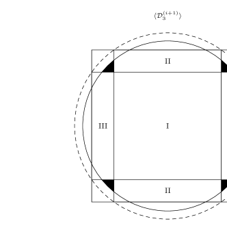
Figure 7.3: $\mathcal{D}_{3}^{(i)}-\mathcal{D}_{3}^{(i+1)}$ plane with the stronger bound given by the circle with radius $\sqrt{5/2}$ which strengthens the less strong bound with radius $\sqrt{3}$ that is given by the dashed circle.

Theorem 2. For the case where each observer chooses between two settings all three-qubit states obey the following inequality:

$$\langle\mathcal{D}_{3}^{(i)}\rangle^{2}+\langle\mathcal{D}_{3}^{(i+1)}\rangle^{2}\leq\frac{5}{2},\leavevmode\nobreak\ \leavevmode\nobreak\ \leavevmode\nobreak\ \forall\rho,$$ (7.23)

for $i=1,2,3$ and where $i$ and $i+1$ are both modulo 3.

Proof: The proof uses the exact same steps as the proof of (7.22) by sun and can be easily performed, although the left hand side of (7.23) contains only two terms instead of the three terms in the left hand side of (7.22). This results in only a minor change in calculations. Case (3) in this proof then has the highest bound of $5/2$, whereas the other three cases give a lower bound equal to $2$. $\square$

Note that in contrast to (7.22) the inequality of (7.23) can not be saturated by separable states, since the latter have a maximum of 2 for the left hand expression in (7.23).

If we again look at the space given by the coordinates $\mathcal{D}_{3}^{(i)}$ (for $i=1,2,3$), we have thus found that all states are, firstly, confined within the intersection of the three orthogonal cylinders $\langle\mathcal{D}_{3}^{(i)}\rangle^{2}+\langle\mathcal{D}_{3}^{(i+1)}\rangle^{2}\leq 5/2$ (with $i+1$ and $i+2$ both modulo $3$) each with radius $\sqrt{5/2}$ and, secondly, they must furthermore still lie within the cube of edge length $2\sqrt{2}$, and thirdly they must also lie within the sphere with radius $\sqrt{3}$. In Figure 7.3 we see the strengthened bound of (7.23) as compared to the bound of sun. However, we see from this figure that neither the intersection of the three cylinders, nor the sphere, nor the cube give tight bounds.

The black areas in Figure 7.3 are non-empty. For the case of (7.23) states thus exist that have both $|\langle D_{3}^{(i)}\rangle|>1$ and $|\langle D_{3}^{(i+1)}\rangle|>1$ (for some $i$). For example, the so-called $W$-state

$$|\,W\rangle=(|\,001\rangle+|\,010\rangle+|\,100\rangle)/\sqrt{3},$$ (7.24)

gives $|\langle D_{3}^{(i)}\rangle|=1.022$ for all $i$ when the observables are chosen as follows: $A_{i}=\cos\alpha_{i}\,\sigma_{z}+\sin\alpha_{i}\,\sigma_{x}$ with $\alpha_{i}=-0.133$ and $A_{i}^{\prime}=\cos\beta_{i}\,\sigma_{z}+\sin\beta_{i}\,\sigma_{x}$ with $\beta_{i}=0.460$.

7.2.2 Restriction to local orthogonal spin observables

roy and uffseev have shown that considerably stronger separability inequalities for the expectation of the bi-partite Bell operator $\mathcal{B}_{2}$ can be obtained if one restricts oneself to local orthogonal observables (LOO’s). See chapter 4. We will now show that the same is the case for the Bell operator $\mathcal{D}_{3}^{(i)}$. The following theorem strengthens all previous bounds of section II for general observables.

Theorem 3. Suppose all local observables are orthogonal, i.e., $\bm{a}_{i}\cdot\bm{a}_{i}^{\prime}=0$, then the following inequalities hold:

(i) For all states: $|\langle\mathcal{D}_{3}^{(i)}\rangle|\leq\sqrt{3/2}$.

(ii) For fully separable states: $|\langle\mathcal{D}_{3}^{(i)}\rangle|\leq\sqrt{3/4}$.

(iii) For bi-separable states in partition $j=1,2,3$:

$$|\langle\mathcal{D}_{3}^{(i)}\rangle|\leq\chi_{i,j}\,,$$ (7.25)

with $\chi_{i,j}=\sqrt{3/2}$ for $i=j$ and $\chi_{i,j}=\sqrt{3/4}$ otherwise.

(iv) Lastly, for all states:

$$\langle D_{3}^{(i)}\rangle^{2}+\langle D_{3}^{(i+1)}\rangle^{2}\leq 2.$$ (7.26)

Proof: (i) The square of $\mathcal{D}_{3}^{(i)}$ is given by

$$(\mathcal{D}_{3}^{(i)})^{2}=(\mathcal{B}_{2}^{(i)})^{2}\otimes\frac{1}{2}(1+\bm{a}_{i}\cdot\bm{a}^{\prime}_{i})\mathds{1}_{i}+\mathds{1}_{2}^{(i)}\otimes\frac{1}{2}(1-\bm{a}_{i}\cdot\bm{a}^{\prime}_{i})\mathds{1}_{i},$$ (7.27)

where $\mathds{1}_{2}^{(i)}$ is the identity operator for the $2$ qubits not including qubit $i$. For orthogonal observables we get $\bm{a}_{i}\cdot\bm{a}^{\prime}_{i}=0$, and $(\mathcal{B}_{2}^{(i)})^{2}\leq 2\mathds{1}_{2}^{(i)}$ (as proven in roy; uffseev). The maximum eigenvalue of $(\mathcal{D}_{3}^{(i)})^{2}$ is thus $3/2$, which implies that $|\langle\mathcal{D}_{3}^{(i)}\rangle|\leq\sqrt{3/2}$.

(ii) For fully separable states we have from (7.18) that

$$\langle\mathcal{D}_{3}^{(i)}\rangle=\frac{1}{2}(\langle\mathcal{B}_{2}^{(i)}\rangle\langle(A_{i}+A_{i}^{\prime})\rangle+\langle(A_{i}-A_{i}^{\prime})\rangle).$$ (7.28)

Furthermore for the case of orthogonal observables $|\langle\mathcal{B}_{2}^{(i)}\rangle|\leq 1/\sqrt{2}$ roy; uffseev. Thus $|\langle\mathcal{D}_{3}^{(i)}\rangle|\leq|(\langle(A_{i}+A_{i}^{\prime})\rangle/\sqrt{2}+\langle(A_{i}-A_{i}^{\prime})\rangle)/2|.$ Since the averages are linear in the state $\rho$ the maximum is obtained for a pure state of qubit $i$. This state can be represented as $1/2(\mathds{1}+\bm{o}\cdot\bm{\sigma})$, with $|\bm{o}|=1$ and $\bm{o}\cdot\bm{\sigma}=\sum_{k}o_{k}\sigma_{k}$ ($k=x,y,z$). Take $C=(A_{i}+A_{i}^{\prime})$, $D=(A_{i}-A_{i}^{\prime})$ and $\bm{s}=\bm{a}_{i}+\bm{a}_{i}^{\prime}$, $\bm{t}=\bm{a}_{i}-\bm{a}_{i}^{\prime}$. We get $|\bm{s}|=|\bm{t}|=\sqrt{2}$. Choose now without losing generality tonerverstraete $\bm{s}=\sqrt{2}(\cos\theta,0,\sin\theta)$ and $\bm{t}=\sqrt{2}(-\sin\theta,0,\cos\theta)$. Then

$$|\langle\mathcal{D}_{3}^{(i)}\rangle| \leq|(\bm{s}\cdot\bm{o}/\sqrt{2}+\bm{t}\cdot\bm{o})/2|$$

$$=|\frac{1}{2}\big{(}(o_{z}-\sqrt{2}o_{x})\sin\theta+(o_{x}+\sqrt{2}o_{z})\cos\theta|\big{)}.$$

Maximizing over $\theta$ (i.e., $\max_{\theta}(X\cos\theta+Y\sin\theta)=\sqrt{X^{2}+Y^{2}}$) and using $o_{x}^{2}+o_{y}^{2}+o_{z}^{2}=1$ we finally get

$$|\langle\mathcal{D}_{3}^{(i)}\rangle| \leq|\sqrt{3/4(o_{x}^{2}+o_{z}^{2})}|\leq\sqrt{3/4}.$$ (7.29)

(iii) For bi-separable states in partition $j=i$ we get the same as in (7.28), but now $|\langle\mathcal{B}_{2}^{(i)}\rangle|\leq\sqrt{2}$. Using the method of (ii) we get

$$|\langle\mathcal{D}_{3}^{(i)}\rangle| \leq|(\sqrt{2}\,\bm{s}\cdot\bm{o}+\bm{t}\cdot\bm{o})/2|\leq\sqrt{3/2}.$$ (7.30)

For bi-separable states in partition $i+1$ and $i+2$ a somewhat more elaborate proof is needed. Let us set $i=1$ and $j=3$ for convenience (for the other partition $j=2$ we get the same result). The maximum is again obtained for pure states. Every pure state in partition $j=3$ can be written as $|\,\psi\rangle=|\,\psi\rangle_{12}\otimes|\,\psi\rangle_{3}$. Then

$$|\langle\mathcal{D}_{3}^{(i)}\rangle|=\,| \frac{1}{4}\langle(A_{1}+A_{1}^{\prime})(A_{2}+A_{2}^{\prime})\rangle_{|\,\psi_{12}\rangle}\langle A_{3}\rangle_{|\,\psi_{3}\rangle}$$

$$+\frac{1}{4}\langle(A_{1}+A_{1}^{\prime})(A_{2}-A_{2}^{\prime})\rangle_{|\,\psi_{12}\rangle}\langle A_{3}^{\prime}\rangle_{|\,\psi_{3}\rangle}+\frac{1}{2}\langle(A_{1}-A_{1}^{\prime})\otimes\mathds{1}_{2}\rangle_{|\,\psi_{12}\rangle}|$$ (7.31)

Using the technique in (ii) above it is found that the maximum over $|\,\psi_{3}\rangle$ gives

$$|\langle\mathcal{D}_{3}^{(i)}\rangle|\leq\,|\frac{\sqrt{2}}{4}\,\big{(}\,\langle(A_{1}+A_{1}^{\prime})\,A_{2}\rangle_{|\,\psi_{12}\rangle}^{2} +\langle(A_{1}+A_{1}^{\prime})\,A_{2}^{\prime}\rangle_{|\,\psi_{12}\rangle}^{2}\,\big{)}^{1/2}$$

$$+\frac{1}{2}\langle(A_{1}-A_{1}^{\prime})\otimes\mathds{1}_{2}\rangle_{|\,\psi_{12}\rangle}|.$$ (7.32)

Without losing generality we choose $A_{i}$, $A_{i}^{\prime}$ in the $x-z$ plane tonerverstraete and $|\,\psi\rangle_{12}=\cos\theta|\,01\rangle+\sin\theta|\,10\rangle$. We can use the symmetry to set $A_{1}=A_{2}=A$ and $A_{1}^{\prime}=A_{2}^{\prime}=A^{\prime}$. This gives

$$|\langle\mathcal{D}_{3}^{(i)}\rangle|\leq\,|\frac{1}{2}(a_{z}-a_{z}^{\prime})\cos(2\theta)+\frac{\sqrt{2}}{4}\big{(}(a_{z}+a_{z}^{\prime})^{2}+((a_{x}+a_{x}^{\prime})^{2}\sin(2\theta))^{2}\big{)}^{1/2}|.$$ (7.33)

Since the observables $A$ and $A^{\prime}$ must be orthogonal (i.e., $\bm{a}\cdot\bm{a}^{\prime}=0$), this expression obtains its maximum for $a_{x}=a_{x}^{\prime}=1/\sqrt{2}$ and $a_{z}=-a_{z}^{\prime}=1/\sqrt{2}$. We finally get:

$$|\langle\mathcal{D}_{3}^{(i)}\rangle|\leq\frac{\sqrt{2}}{2}\cos(2\theta)+\frac{1}{2}\sin(2\theta)\leq\sqrt{3/4}.$$ (7.34)

(iv) We use the exact same steps of the proof of Sun & Fei of (7.22) (i.e., sun) but since the observables are orthogonal only case (4) of that proof needs to be evaluated. This can be easily performed for the left hand side of (7.26) that contains only two terms instead of the three terms on the right hand side of (7.22), thereby resulting in only a minor modification of the calculations giving the result $\langle D_{3}^{(i)}\rangle^{2}+\langle D_{3}^{(i+1)}\rangle^{2}\leq 2$. $\square$

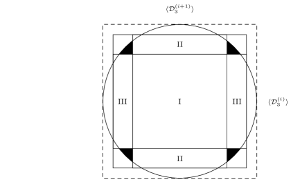
Figure 7.4: The results of Theorem 3 for orthogonal observables. For comparison to the case where the observables were not restricted to be orthogonal, the dashed square is included that has edge length $2\sqrt{2}$ and which is the largest square in Figure 7.3.

These results for orthogonal observables can again be interpreted in terms of the space given by the coordinates $\mathcal{D}_{3}^{(i)}$ (for $i=1,2,3$). The same structure as in Figure 7.3 then arises but with the different numerical bounds of Theorem 2. The fully separable states are confined to a cube with edge length $\sqrt{3}$ and the bi-separable states in partition $j=1,2,3$ are confined to cuboids with size either $\sqrt{6}\times\sqrt{3}\times\sqrt{3},\leavevmode\nobreak\ \sqrt{3}\times\sqrt{6}\times\sqrt{3}$, or $\sqrt{3}\times\sqrt{3}\times\sqrt{6}$. Furthermore, all three-qubit states are in the intersection of firstly the cube with edge length $\sqrt{6}$, secondly of the three orthogonal cylinders with radius $\sqrt{2}$, and thirdly of the sphere with radius $\sqrt{3}$.

The corresponding $\mathcal{D}_{3}^{(i)}-\mathcal{D}_{3}^{(i+1)}$ plane is drawn in Figure 7.4. Compared to the case where no restriction was made to orthogonal observables (cf. Figure 7.3) we see that we can still distinguish the different kinds of bi-separable states, but they can still not be distinguished from fully three-partite entangled states since both types of states still have the same maximum for $\langle\mathcal{D}_{3}^{(i)}\rangle$. Furthermore, the ratio of the different maxima of $\langle\mathcal{D}_{3}^{(i)}\rangle$ for fully separable and bi-separable states is still the same, i.e., the ratio is $\sqrt{2}/1=(\sqrt{3/2})/(\sqrt{3/4})=\sqrt{2}$.

The black areas in Figure 7.4 are again non-empty since states exist that have both $|\langle D_{3}^{(i)}\rangle|>\sqrt{3/4}$ and $|\langle D_{3}^{(i+1)}\rangle|>\sqrt{3/4}$ for the case of orthogonal observables. For example, the $W$-state of (7.24) gives $|\langle D_{3}^{(i)}\rangle|=0.906$ for all $i$, for the local angles $\alpha_{i}=0.54=\beta_{i}-\pi/2$ in the $x$-$z$ plane.

7.2.3 Discussion of the monogamy aspects

Let us take another look at the quadratic inequalities $\langle D_{3}^{(i)}\rangle^{2}+\langle D_{3}^{(i+1)}\rangle^{2}\leq 5/2$ of (7.23) for general observables and $\langle D_{3}^{(i)}\rangle^{2}+\langle D_{3}^{(i+1)}\rangle^{2}\leq 2$ of (7.26) for orthogonal observables. These can be interpreted as monogamy inequalities for maximal bi-separable three-qubit quantum correlations (i.e., bi-separable correlations that saturate the inequalities), since the inequalities show that a state that has maximal bi-separable correlations for a certain partition can not have it maximally for another partition. Indeed, when partition $i$ gives $|\langle D_{3}^{(i)}\rangle|=\sqrt{2}$ it must be the case according to (7.23) that for the other two partitions both $|\langle D_{3}^{(i+1)}\rangle|\leq\sqrt{1/2}$ and $|\langle D_{3}^{(i+2)}\rangle|\leq\sqrt{1/2}$ must hold. The latter two must thus be non-maximal as soon as the first type of bi-separable correlation is maximal. And for the second inequality of (7.26) using orthogonal observables we get that when $|\langle D_{3}^{(i)}\rangle|=\sqrt{3/2}$ (this is maximal) it must be the case that both $|\langle D_{3}^{(i+1)}\rangle|\leq\sqrt{1/2}$ and $|\langle D_{3}^{(i+2)}\rangle|\leq\sqrt{1/2}$, which is non-maximal.

From this we see that the first (i.e., (7.23) for general observables) is a stronger monogamy relationship than the second (i.e., (7.26) for orthogonal observables) in the sense that the trade-off between how much the maximal value for $|\langle D_{3}^{(i)}\rangle|$ for one partition $i$ restricts the value of $|\langle D_{3}^{(i+1)}\rangle|$, $|\langle D_{3}^{(i+2)}\rangle|$ for the other two partitions below the maximal value is larger in the first case than in the second case.

Let us see how this compares to the Toner-Verstraete monogamy inequality $\langle\mathcal{B}^{(i)}_{2}\rangle^{2}+\langle\mathcal{B}^{(i+1)}_{2}\rangle^{2}\leq 2$ of (7.1). Here $|\langle\mathcal{B}^{(i)}_{2}\rangle_{\textrm{lhv}}|\leq 1$ is the ordinary CHSH inequality (scaled down by a factor of $2$) for the local correlations of the two qubits other than qubit $i$ (cf. (7.1)). The Toner-Verstraete monogamy inequality is even stronger than the ones presented here, because when $|\langle\mathcal{B}^{(i)}_{2}\rangle|$ obtains its maximal value of $\sqrt{2}$ it must be that $|\langle\mathcal{B}^{(i+1)}_{2}\rangle|$=$|\langle\mathcal{B}^{(i+2)}_{2}\rangle|=0$.

Furthermore, in section 7.1.2 we have seen that the Toner-Verstraete monogamy relationship shows that the non-locality indicated by correlations that violate the CHSH inequality cannot be shared: as soon as for some $i$ one has $|\langle\mathcal{B}^{(i)}_{2}\rangle|>1$, it must be that both $|\langle\mathcal{B}^{(i+1)}_{2}\rangle|<1$ and $|\langle\mathcal{B}^{(i+2)}_{2}\rangle|<1$. But we have also seen that collinsgisin have nevertheless shown that the quantum non-locality indicated by a violation of the bi-partite Bell-type inequality (7.16) indicates can be shared. Since $|\langle D_{3}^{(i)}\rangle_{\textrm{lhv}}|\leq 1$ are local Bell-type inequalities (see (7.17)) whose violation can be seen to indicate some non-locality, the inequalities considered here could possibly also indicate some quantum non-locality sharing. Indeed, this is the case since it was shown that the black areas in Figure 7.3 are non-empty. Violation of the Bell-type inequalities given here thus indicate shareability of the non-locality of bi-separable three-qubit quantum correlations.

In conclusion, we have presented stronger bounds for bi-separable correlations in three-partite systems than were given by sun and extended this analysis to the case of the restriction to orthogonal observables which gave even stronger bounds. The quadratic inequalities for bi-separable correlations give a monogamy relationship for correlations that violate these inequalities maximally (i.e., such correlations cannot be shared), but they indicate shareability of the non-maximally violating correlations.

We hope that future research will reveal more of the monogamy of multi-partite quantum correlations. It could therefore be fruitful to generalize this work from three to a larger number of parties. Even more interesting would be including also no-signaling correlations besides correlations that come from quantum states.

7.3 Discussion

In this chapter we have seen that, apart from using Bell-type inequalities in terms of all parties involved, another fruitful way of studying the different kinds of correlations is via the question whether the correlations can be shared. Here one focuses on subsets of the parties and whether their correlations can be extended to parties not in the original subsets. This can be done either directly in terms of joint probability distributions or in terms of relations between Bell-type inequalities that hold for different, but overlapping subsets of the parties involved.

We have proven that unrestricted general correlations can be shared to any number of parties (called $\infty$-shareable). In the case of no-signaling correlations it was already known that such correlations can be $\infty$-shareable iff the correlations are local. We have shown that this implies, firstly, that partially-local correlations are also $\infty$-shareable, since they are combinations of local and unrestricted correlations between subsets of the parties. Secondly, it implies that both quantum and no-signaling correlations that are non-local are not $\infty$-shareable and we have shown monogamy constraints for such correlations.

We have investigated the relationship between sharing non-local quantum correlations and sharing mixed entangled states, and already for the simplest bi-partite correlations this was shown to be non-trivial. The Collins-Gisin Bell-type inequality indicates that non-local quantum correlations can be shared and it thus indicates sharing of entanglement of mixed states. The CHSH inequality was shown not to indicate this. This shows that non-local bi-partite correlations in a setup with two-dichotomous observables per party cannot be shared, whereas this is possible in a setup with one observable per party more.

We have given a simpler proof of the monogamy relation $\langle\mathcal{B}_{ab}\rangle_{\textrm{qm}}^{2}+\langle\mathcal{B}_{ac}\rangle_{\textrm{qm}}^{2}\leq 8$ of tonerverstraete. We have furthermore provided a different strengthening of this constraint than the one given by Toner and Verstraete. For no-signaling correlations we have argued that the monogamy constraint $|\langle\mathcal{B}_{ab}\rangle_{\textrm{ns}}|+|\langle\mathcal{B}_{ac}\rangle_{\textrm{ns}}|\leq 4$ of toner2 can be interpreted as a non-trivial bound on the set of three-partite no-signaling correlations. This discerning inequality uses product expectation values only. We know of no other such non-trivial bounds for no-signaling correlations of three or more parties (in the next chapter this will be further discussed).

Lastly, we have derived monogamy constraints for three-qubit bi-separable quantum correlations, which is a first example of investigating monogamy of quantum correlations using a three-partite Bell-type inequality.

Chapter 8 Discerning multi-partite partially-
local, quantum mechanical and
no-signaling correlations

This chapter is in part based on seevsvet.

8.1 Introduction

In the previous chapters we have seen that quadratic and linear Bell-type inequalities distinguish the correlations of various types of multi-partite quantum states. We have also we seen that Mermin-type inequalities discern LHV models from quantum mechanics, i.e., they discern local correlations from quantum correlations. In this chapter we will construct new Bell-type inequalities to discern partially-local from quantum mechanical correlations and also discuss the issue of discerning multi-partite no-signaling correlations. Unfortunately, the Mermin-type inequalities do not suffice for either purpose.

Let us recall the notion of partial locality by reviewing some of the definitions that were given in chapter 2. For $N=2$ locality and partial locality coincide so we start our investigation at $N=3$. Here we consider three-partite models where arbitrary correlations (e.g., a signaling correlation) are allowed between two of the three parties but only local correlations between these two and the third party. The two parties that are non-locally correlated need not be fixed in advance, but can be chosen with probability $p_{i}$. The correlations (joint probability distributions) are thus of the form

$$P(a_{1},a_{2},a_{3}|A_{1},A_{2},A_{3})=\int_{\Lambda}d\lambda\,[\, p_{1}\,\rho_{1}(\lambda)P_{1}(a_{1}|A_{1},\lambda)P_{1}(a_{2},a_{3}|A_{2},A_{3},\lambda)$$

$$+p_{2}\,\rho_{2}(\lambda)P_{2}(a_{2}|A_{2},\lambda)P_{2}(a_{1},a_{3}|A_{1},A_{3},\lambda)$$

$$+p_{3}\,\rho_{3}(\lambda)P_{3}(a_{3}|A_{3},\lambda)P_{3}(a_{1},a_{2}|A_{1},A_{2},\lambda)\,].$$ (8.1)

with $A_{i}$ observables and $a_{i}$ outcomes and where $P_{1}(a_{2},a_{3}|A_{2},A_{3},\lambda)$ can be any probability distribution; it need not factorise into $P_{1}(a_{2}|A_{2},\lambda)P_{1}(a_{3}|A_{3},\lambda)$. Analogously for the other two joint probability terms. The $\rho_{i}(\lambda)$ are the hidden-variable distributions. Models that allow for correlations of the form (8.1) are called partially-local hidden-variable models (PLHV) models. Models whose correlations cannot be written in this form are fully non-local, i.e., they are said to contain full non-locality.

For the three-partite case svetlichny derived a non-trivial Bell-type inequality for partially-local correlations of the form (8.1). This inequality can thus distinguish between full three-partite non-locality and two-partite non-locality in a three-partite system. A priori it is not clear if the correlations of the form (8.1) are stronger than quantum mechanical correlations. However, Svetlichny showed that quantum states exist that give correlations that violate the inequality, thereby proving that these correlations are fully non-local. Furthermore, no-signaling correlations were shown to violate the inequality maximally jones; barrett05. Thus three-partite quantum and no-signaling correlations exist that cannot be reproduced by any three-partite PLHV model, despite the fact that PLHV models allow for arbitrary strong signaling correlations between any two of the three parties.

In this chapter we generalize Svetlichny’s inequalities to the multi-partite case and we call them Svetlichny inequalities. Quantum mechanics violates these inequalities for some fully entangled multi-qubit states and these thus contain fully non-local correlations. In a recent four particle experiment such a violation was observed, so full non-locality occurs in nature. It is an open question whether all fully entangled states imply full non-locality. If they do, this cannot always be shown by violations of the Svetlichny inequalities, because we will show that fully entangled states exist that do not violate any of them.

After we announced the multi-partite generalization of Svetlichny’s three-partite inequality, as published in seevsvet, collins independently also presented such a generalization. CER commented upon the original three-partite case, and jones performed an extension of the generalization and furthermore showed that no-signaling correlations can give maximal violation of the Svetlichny inequalities.

The outline of this chapter is as follows. In section 8.2 some preliminary results and notations are presented. In section 8.3 the three-partite case is treated as a stepping stone to the multi-partite generalization of section 8.4. In presenting the three-partite case we use the presentation as in collins and CER. For the multi-partite generalization we use the original proof given by us, and present some further multi-partite results by jones. In section 8.5 we look at some further aspects of quantum mechanical violations of the generalized Svetlichny inequalities. In section 8.6 we comment on the fact that although the Svetlichny inequalities discern partially-local and quantum correlations from the most general correlations, they cannot do so for no-signaling correlations. What set of inequalities that bound some linear sum of product expectation values (possibly including some marginal expectation values) and that would discern the multi-partite no-signaling correlations, we pose as an interesting open problem. Lastly, in section 8.7 we give a conclusion and discussion of the results obtained.

8.2 Preliminaries

In order to introduce the Svetlichny inequality and to give its multi-partite generalization in the next section it is helpful to introduce the so-called Mermin polynomials, whose quantum counterpart we have already encountered in chapter 5.4 and that were used to give the Mermin-type separability inequalities (6.8). Let $A_{j}$ and $A_{j}^{\prime}$ be dichotomic observables for parties $j=1,\ldots N$. The Mermin polynomials are defined in the following way: Let $M_{2}=A_{1}A_{2}+A_{1}^{\prime}A_{2}+A_{1}A_{2}^{\prime}-A_{1}^{\prime}A_{2}^{\prime}$ (i.e., analogous to the Bell operator $\mathcal{B}$), and define recursively

$$M_{j}:=\frac{1}{2}(M_{j-1}(A_{j}+A_{j}^{\prime})+M_{j-1}^{\prime}(A_{j}-A_{j}^{\prime})),$$ (8.2)

where for $M_{j}^{\prime}$ all primed and non-primed observables are exchanged. For $N=3$ we get

$$M_{3}:= A_{1}^{\prime}A_{2}A_{3}+A_{1}A_{2}^{\prime}A_{3}+A_{1}A_{2}A_{3}^{\prime}-A_{1}^{\prime}A_{2}^{\prime}A_{3}^{\prime},$$ (8.3)

$$M_{3}^{\prime}:= A_{1}A_{2}^{\prime}A_{3}^{\prime}+A_{1}^{\prime}A_{2}A^{\prime}_{3}+A_{1}^{\prime}A^{\prime}_{2}A_{3}-A_{1}A_{2}A_{3}.$$ (8.4)

In the following we consider expectation values of these polynomials as predicted by the different types of correlations as distinguished in chapter 2. That is, we consider the expectation values $\langle M_{N}\rangle_{\textrm{plhv}}$, $\langle M_{N}\rangle_{\textrm{qm}}$ and $\langle M_{N}\rangle_{\textrm{ns}}$. Furthermore, the absolute maximum on $\langle M_{N}\rangle$ is denoted by $|M_{N}|_{\textrm{max}}$ and is equal to the number of terms in the Mermin polynomial. It is always possible to find a fully non-local model that is able to give this absolute maximum.

gisin were the first to derive that $|\langle M_{N}\rangle_{\textrm{lhv}}|\leq 2$, $|\langle M_{N}\rangle_{\textrm{qm}}|\leq 2^{(N+1)/2}$, $|M_{N}|_{\textrm{max}}=2^{(N+1)/2}$ for $N$ = odd, and $|M_{N}|_{\textrm{max}}=2^{N/2}$ for $N$ = even. It was shown in chapter 5.4 that the tight quantum bounds on Mermin polynomials distinguish various forms of entanglement including full entanglement. An interesting question now is if these polynomials are also suitable for detecting full multi-partite non-locality. For this purpose one needs to find the bounds on $\langle M_{N}\rangle_{\textrm{plhv}}$ so as to answer if one can use some Mermin-type inequality to distinguish a partially-local from a fully non-local model. It will be shown that for $N$ = even that this is indeed the case, but not for $N$ = odd. Consequently, for $N$ = odd new inequalities need to be found. Svetlichny provided the case $N=3$, which we will review in the next section. Later we will generalize his inequality to all $N$.

8.3 Three-partite partial locality

Consider the Mermin polynomial $M_{3}$. For this case $\max|\langle M_{3}\rangle_{\textrm{qm}}|=|M_{3}|_{\textrm{max}}=4$. We want to determine $\max|\langle M_{3}\rangle_{\textrm{plhv}}|$. collins obtained this as follows. Consider the recursive relation (8.2) so as to obtain $M_{3}=(M_{2}(A_{3}+A_{3}^{\prime})+M_{2}^{\prime}(A_{3}-A_{3}^{\prime}))/2$. Now assume partial factorisability in the sense that party $3$ factorises from party $1$ and $2$. We note that this is not a limiting restriction because the same results follows for the two other choices or convex combinations of these three possibilities. The desired maximum becomes: $\max|\langle M_{3}\rangle_{\textrm{plhv}}|=\max|\,|M_{2}|_{\textrm{max}}\langle A_{3}+A_{3}^{\prime}\rangle+|M_{2}|_{\textrm{max}}\langle A_{3}-A_{3}^{\prime}\rangle|/2$. Here the absolute maxima for the expectation values of $M_{2}$ and $M_{2}^{\prime}$ can be attained since arbitrary strong correlations between party $1$ and $2$ are allowed. Since we are dealing with dichotomic observables with outcomes $\pm 1$, the maximum of $|\langle M_{3}\rangle_{\textrm{plhv}}|$ is obtained if $|\langle A_{3}\rangle|=|\langle A_{3}^{\prime}\rangle|=1$. Without loss of generality we choose $\langle A_{3}\rangle=\langle A_{3}^{\prime}\rangle=1$ so that $\max|\langle M_{3}\rangle_{\textrm{plhv}}|=|M_{2}|_{\textrm{max}}=|M_{3}|_{\textrm{max}}=4$. In conclusion, we have obtained the tight bound

$$|\langle M_{3}\rangle_{\textrm{plhv}}|,|\langle M_{3}\rangle_{\textrm{qm}}|\leq|M_{3}|_{\textrm{max}}=4,$$ (8.5)

from which it follows that $M_{3}$ does not distinguish between PLHV models, quantum mechanics and models that allow for full unrestricted non-locality between all parties.

The problem lies in the fact that $M_{3}$ only has four correlation terms. CER showed that a PLHV model with correlations as in (8.1) can reproduce whatever values are assumed for the four expectation values in $M_{3}$. Likewise another such PLHV model can be found that reproduces the expectation values in $M_{3}^{\prime}$. Thus, in order to give a non-trivial bound for PLHV models one needs to consider at least more than four product expectation values. Svetlichny considered all eight possible terms using the following two polynomials:

$$S^{\pm}_{3}:=M_{3}\pm M_{3}^{\prime}.$$ (8.6)

We call these Svetlichny polynomials. Both polynomials have eight terms from which one obtains $|S_{3}^{\pm}|_{\textrm{max}}=8$. Using the recursive relation (8.2) we see that $S_{3}^{\pm}$ is equal to $M_{2}A_{3}^{\prime}\pm M_{2}^{\prime}A_{3}$. Then for the case of partial factorisability where party $3$ factorises from party $1$ and $2$ one obtains that the maximum of $|\langle S_{3}^{\pm}\rangle_{\textrm{plhv}}|$ is given by $|M_{2}\pm M_{2}^{\prime}|_{\textrm{max}}=2|A_{1}A_{2}^{\prime}\pm A_{1}^{\prime}A_{2}|_{\textrm{max}}=4$, which is half the absolute maximum $|S_{3}^{\pm}|_{\textrm{max}}=8$. This finally gives a non-trivial inequality: all PLHV models that allow correlations of the form (8.1) must obey the following non-trivial bound

$$|\langle S^{\pm}_{3}\rangle_{\textrm{plhv}}|\leq 4.$$ (8.7)

Explicitly the inequalities read:

$$|\langle S_{3}^{\pm}\rangle|= |\langle A_{1}A_{2}A_{3}\rangle\pm\langle A_{1}A_{2}A_{3}^{\prime}\rangle\pm\langle A_{1}A_{2}^{\prime}A_{3}\rangle\pm\langle A_{1}^{\prime}A_{2}A_{3}\rangle$$

$$-\langle A_{1}A_{2}^{\prime}A_{3}^{\prime}\rangle-\langle A_{1}^{\prime}A_{2}A_{3}^{\prime}\rangle-\langle A_{1}^{\prime}A_{2}^{\prime}A_{3}\rangle\pm\langle A_{1}^{\prime}A_{2}^{\prime}A_{3}^{\prime}\rangle|\leq 4,$$ (8.8)

These are necessary conditions to be obeyed by all three-partite PLHV models.

Since $\langle S_{3}^{+}\rangle^{2}+\langle S_{3}^{-}\rangle^{2}=2(\langle M_{3}\rangle^{2}+\langle M_{3}^{\prime}\rangle^{2})$ we obtain from the Mermin-type separability inequalities (6.8) that the maximum value attainable by quantum mechanics is $\max|\langle S^{\pm}_{3}\rangle_{\textrm{qm}}|=4\sqrt{2}$. This is attained for a GHZ state, as first shown by svetlichny. Quantum mechanics thus contains states that have full non-locality.

In conclusion, Svetlichny obtained the following bounds:

$$2\max|\langle S^{\pm}_{3}\rangle_{\textrm{plhv}}|=\sqrt{2}\max|\langle S^{\pm}_{3}\rangle_{\textrm{qm}}|=|S^{\pm}_{3}|_{\textrm{max}}=8.$$ (8.9)

The three bounds are each time increased with a factor $\sqrt{2}$. In the next section we give the multi-partite generalization of these bounds. It is noteworthy that no-signaling correlations can reach the absolute maximum jones: $\max|\langle S^{\pm}_{3}\rangle_{\textrm{ns}}|=|S^{\pm}_{3}|_{\textrm{max}}$. This means that the Svetlichny polynomials cannot be used to distinguish three-partite no-signaling correlations from more general correlations that are signaling. This will be further commented upon in section 8.6.

To end this section we mention that it is an open question what is the minimum number of correlation terms one should consider in a Svetlichny-like polynomial in order to distinguish between bi-partite non-locality and full three-partite non-locality. We have seen that four terms does not suffice, whereas eight terms does suffice, but perhaps one can do with less.

8.4 Generalization to $N$-partite partial locality

For four parties the strategy of the previous section gives

$$\max|\langle M_{4}\rangle_{\textrm{plhv}}|=4,\leavevmode\nobreak\ \max|\langle M_{4}\rangle_{\textrm{qm}}|=4\sqrt{2},\leavevmode\nobreak\ \textrm{whereas}\leavevmode\nobreak\ |M_{4}|_{\textrm{max}}=8,$$ (8.10)

and analogously for $M_{4}^{\prime}$. This shows that for four parties the Mermin polynomial gives non-trivial bounds on PLHV models. Let us now generalize this by showing that (up to a numerical factor) the Mermin polynomials $M_{N}$ and $M_{N}^{\prime}$ for $N$ = even give valid Svetlichny inequalities that test partial factorisability. However, just as was the case for $N=3$ it will be shown that for $N$ = odd one should take a linear combination of the two Mermin polynomials $M_{N}$ and $M_{N}^{\prime}$.

Consider an $N$-partite system and let us now make the following partial factorisability assumption (we recall this from chapter 2): An ensemble of such systems consists of subensembles in which each one of the subsets of the $N$ parties form extended systems, whose subsystems can be correlated in any way (e.g., entangled, fully non-local) which however are uncorrelated to each other. Let us for the time being focus our attention on one of these subensembles, formed by a system consisting of two subsystems of $k<N$ and $N-k<N$ parties which are uncorrelated to each other. Assume also for the time being that the first subsystem is formed by parties $1,2,\dots,k$ and the other by the remaining. We express our partial factorisability hypothesis by assuming a factorisable expression for the probability $p(a_{1},a_{2},\ldots,a_{N}|A_{1},A_{2},\cdots,A_{N})$ for observing the results $a_{i}$, for the observables $A_{i}$:

$$p(a_{1},a_{2},\ldots,a_{N}|A_{1},A_{2},\ldots,A_{N})=$$

$$\int P(a_{1},\ldots,a_{k}|A_{1},\ldots,A_{k},\lambda)P(a_{k+1},\ldots,a_{N}|A_{k+1},\ldots,A_{N},\lambda)\,\rho(\lambda)\,d\lambda,$$ (8.11)

where the probabilities are conditioned to the hidden variable $\lambda$ with probability measure $d\rho$. Formulas similar to (8.11) with different choices of the composing parties and different value of $k$ describe the other subensembles. We need not consider decomposition into more than two subsystems as then any two can be considered jointly as parts of one subsystem still uncorrelated with respect to the others.

Consider the expectation value of the product of the observables in the original ensemble

$$\langle A_{1}A_{2}\cdots A_{N}\rangle_{\textrm{plhv}}=\sum_{J}(-1)^{n(J)}p(J),$$

where $J$ stands for an $N$-tuple $j_{1},\dots,j_{N}$ with $j_{k}=\pm 1$, $n(J)$ is the number of $-1$ values in $J$ and $p(J)$ is the probability of achieving the indicated values of the observables. Using the hypothesis of Eq. (8.11) as a constraint we now derive non-trivial inequalities satisfied by the numbers $\langle A_{1}A_{2}\cdots A_{N}\rangle_{\textrm{plhv}}$ when introducing two alternative dichotomic observables $A_{i}^{1},A_{i}^{2}$, $i=1,2,\dots,N$ (here we write $A^{1}_{i}$ and $A^{2}_{i}$ instead of $A_{i}$ and $A^{\prime}_{i}$ for the dichotomic observables for party $i$). To simplify the notation we write $\langle i_{1}i_{2}\cdots i_{N}\rangle_{\textrm{plhv}}$ for $\langle A_{1}^{i_{1}}A_{2}^{i_{2}}\cdots A_{N}^{i_{N}}\rangle_{\textrm{plhv}}$, where $i_{1}=1,2$ denotes which of the two dichotomic observables is chosen for party $1$, etc. For any value of $k$ and any choice of these $k$ parties to comprise one of the subsystems we obtain (proof in the Appendix on page 8) the following inequalities:

$$\sum_{I}\nu^{\pm}_{t(I)}\langle i_{1}i_{2}\cdots i_{N}\rangle_{\textrm{plhv}}\leq 2^{N-1},$$ (8.12)

where $I=(i_{1},i_{2},\dots,i_{N})$, $t(I)$ is the number of times index $2$ appears in $I$, and $\nu^{\pm}_{k}$ is a sequence of signs given by

$$\nu^{\pm}_{k}=(-1)^{\frac{k(k\pm 1)}{2}}.$$ (8.13)

These sequences have period four with cycles $(1,-1,-1,1)$ and $(1,1,-1,-1)$ respectively. We call these inequalities alternating. They are direct generalizations of the three-partite inequalities by svetlichny. The alternating inequalities are satisfied by a system with any form of partial factorisability, so their violation is a sufficient indication of full non-factorisability.

Introduce now the operator

$$S_{N}^{\pm}=\sum_{I}\nu_{t(I)}^{\pm}A_{1}^{i_{1}}\cdots A_{N}^{i_{N}}.$$ (8.14)

Using Eq. (8.12) the $N$-partite alternating inequalities can be expressed as

$$|\langle S^{\pm}_{N}\rangle_{\textrm{plhv}}|\leq 2^{N-1}.$$ (8.15)

For even $N$ the two inequalities are interchanged by a global change of labels $1$ and $2$ and are thus equivalent. However for odd $N$ this is not the case and thus they must be considered a-priori independent. To see this consider the effect of such a change upon the cycle $(1,-1,-1,1)$. If $N$ is even, we get $(-1)^{N/2}(1,1,-1,-1)$ which gives the second alternating inequality. For $N$ = odd, we get $\pm(1,-1,-1,1)$, which results in the same inequality. Similar results hold for the other cycle. The inequalities (8.15) are necessary conditions for a PLHV model to exist. It is not known what a necessary and sufficient set would be.

The bound (8.15) for PLHV models is sharp since it can be obtained by considering for example the bi-separable partition $\{1,\ldots,N-1\}\,,\,\{N\}$ and choosing the absolute maximum for $S_{N-1}^{\pm}$, which is $2^{N-1}$ since there are just that many terms in the operator $S_{N-1}^{\pm}$, and choosing $\langle A_{N}\rangle=\langle A_{N}^{\prime}\rangle=1$ for party $N$.

Let us consider the Svetlichny polynomials at closer scrutiny. The following recursive relation holds:

$$S_{N}^{\pm}=S_{N-1}^{\pm}A_{N}\mp S_{N-1}^{\mp}A_{N}^{\prime},$$ (8.16)

with $S_{2}^{+}=-M_{2}$ and $S_{2}^{-}=M_{2}^{\prime}$ . Consider the term $S_{N-1}^{\pm}A_{N}$. The maximum of $|\langle S_{N-1}^{\pm}A_{N}\rangle|$ is equal to the maximum of $|\langle S_{N-1}^{\pm}\rangle|$ since $\max|\langle A_{N}\rangle|=1$. Similarly for the other term. Thus one can take the $N$-partite bound as twice the $(N-1)$-partite bound.

The Svetlichny polynomials $S_{N}$ are related to the Mermin polynomials $M_{N}$ by the following linear recursive relations uffink:

$$S^{\pm}_{N}=2^{l-1}\left((-1)^{l(l\pm 1)/2}M_{N}\mp(-1)^{l(l\mp 1)/2}M^{\prime}_{N}\right),\leavevmode\nobreak\ \leavevmode\nobreak\ \leavevmode\nobreak\ \leavevmode\nobreak\ \textrm{for}\leavevmode\nobreak\ N\textrm{ = odd, and }N=2\,l+1,$$

$$S^{\pm}_{N}=2^{l-1}(-1)^{l(l\pm 1)/2}M_{N}^{\pm}, \textrm{for}\leavevmode\nobreak\ N\textrm{ = even, and }N=2\,l,$$ (8.17)

where $M_{N}^{+}:=M_{N}$ and $M_{N}^{-}:=M_{N}^{\prime}$.

The expectation values are thus related as:

$$|\langle S_{N}^{\pm}\rangle|=\left\{\begin{array}[]{cc}2^{(N-2)/2}|\langle M_{N}^{\pm}\rangle|,&\textrm{if}\leavevmode\nobreak\ N\textrm{ = even},\\ 2^{(N-3)/2}|\langle M_{N}^{\pm}\pm M_{N}^{\mp}\rangle|,\nobreak\leavevmode\nobreak\leavevmode\nobreak\leavevmode&\textrm{if}\leavevmode\nobreak\ N\textrm{ = odd}.\end{array}\right.$$ (8.20)

Note that from the above relations we get the following identity:

$$\langle S_{N}^{+}\rangle^{2}+\langle S_{N}^{-}\rangle^{2}=2^{N-2}(\langle M_{N}\rangle^{2}+\langle M_{N}^{\prime}\rangle^{2}).$$ (8.21)

Hence, the quadratic separability inequalities of (6.7) for multi-partite quantum states can be equally expressed in terms of operators $S_{N}$. The maximal quantum mechanical violation the left-hand side of the $N$-partite alternating inequalities of (8.15) is thus equal to $2^{N-1}\sqrt{2}$. This upper bound is in fact achieved for the GHZ states for appropriate values of the polarizer angles of the relevant spin observables.

In conclusion, fully entangled quantum states can violate the Svetlichny inequalities by a factor as large as $\sqrt{2}$ seevsvet; collins, thereby proving that quantum correlations contain full multi-partite non-locality. The absolute maximum is a factor $\sqrt{2}$ larger than the maximum quantum bound. Thus

$$2\max|\langle S_{N}\rangle_{\textrm{plhv}}|=\sqrt{2}\max|\langle S_{N}\rangle_{\textrm{qm}}|=|S_{N}|_{\textrm{max}}=2^{N}.$$ (8.23)

Note that quantum mechanics can never attain the absolute maximum for the expectation value of the Svetlichny polynomials $S^{\pm}_{N}$. This is in contradistinction to what was the case for the Mermin polynomials $M_{N}$ and $M_{N}^{\prime}$, where for $N$ = odd quantum mechanics is able to give the absolute maximum on $|\langle M_{N}\rangle_{\textrm{qm}}|$ and $|\langle M_{N}^{\prime}\rangle_{\textrm{qm}}|$. It is thus the quantum bound on the Svetlichny polynomials, and not on the Mermin polynomials that distinguishes quantum correlations from more general correlations for all $N$.

The two alternating solutions for $N=2$ are the usual CHSH inequalities, i.e, $|\langle M_{2}\rangle_{\textrm{lhv}}|\leq 2$, and $|\langle M_{2}\rangle_{\textrm{lhv}}^{\prime}|\leq 2$, where for $N=2$ there is of course no distinction between a LHV and PLHV model. The ones for $N=3$ give rise to the two inequalities found in Svetlichny svetlichny that are also given in (8.7), and for $N=4$ we have $|\langle S_{4}^{+}\rangle_{\textrm{plhv}}|=2|\langle M_{4}\rangle_{\textrm{plhv}}|\leq 8$ and where the second inequality is $|\langle S_{4}^{-}\rangle_{\textrm{plhv}}|=2|\langle M_{4}^{\prime}\rangle_{\textrm{plhv}}|\leq 8$.

8.4.1 Alternative formulation

After seevsvet announced their generalized Svetlichny inequalities collins independently announced similar inequalities. They define the following Svetlichny polynomials

$$\widetilde{S}_{N}=\left\{\begin{array}[]{cc}M_{N},&\textrm{if}\leavevmode\nobreak\ N\textrm{ = even},\\ \frac{1}{2}(M_{N}+M_{N}^{\prime}),\nobreak\leavevmode\nobreak\leavevmode\nobreak\leavevmode&\textrm{if}\leavevmode\nobreak\ N\textrm{ = odd},\end{array}\right.$$ (8.26)

and prove for $N$ = odd: $|\langle\widetilde{S}_{N}\rangle_{\textrm{plhv}}|\leq 2^{(N-1)/2}$, and for $N$ = even: $|\langle\widetilde{S}_{N}\rangle_{\textrm{plhv}}|\leq 2^{(N-2)/2}$. The quantum bounds are a factor $\sqrt{2}$ higher and the absolute maxima $|\widetilde{S}_{N}|_{\textrm{max}}$ are a factor $2$ higher. These bounds give the same structure as in (8.23) which was obtained using the Svetlichny polynomial $S^{\pm}_{N}$ used here. This formulation (8.26) is used by jones and marcovitch.

Although using (8.26) gives a simpler recursive relation in terms of the Mermin polynomials than was the case for $S^{\pm}_{N}$ as given in (8.17), the bounds for $\widetilde{S}_{N}$ now depend on whether $N$ is even or odd, which we regard to be an unwelcome feature.

8.5 Further remarks on quantum mechanical
violations

We have seen that using $N$-partite GHZ states the Svetlichny inequalities can be violated by as large as a factor $\sqrt{2}$. The GHZ states are fully entangled and this full entanglement is a necessary feature to give a violation. This follows from the fact that (6.7) of chapter 5.4 shows (using the identity (8.21)) that any bi-separable state (i.e., $k=2$) has a maximal value for $\langle S_{N}^{\pm}\rangle_{\textrm{qm}}$ equal to $2^{(N-3/2)}$, which is a factor $\sqrt{2}$ below the PLHV bound as given in (8.15). Thus a ‘gap’ appears between the correlations that can be obtained by bi-separable quantum states and those obtainable by PLHV models. It thus takes fully entangled states to obtain all the correlations obtainable by a PLHV model. This is analogous to the results found in section 6.3.3.4 for the LHV case, where it was shown that one needs entangled states to give all the correlations that are producible by LHV models.

These results imply that the mere requirement of locality (factorisability) between just two subsets, although within each subset full blown non-locality is admissible, already forces the correlations to be less strong than some of the quantum mechanical correlations, although they are nevertheless still stronger than those obtainable from bi-separable quantum states.

An interesting question to ask next is whether the $N$-partite non-locality that is found in the fully entangled GHZ states is generic or whether it can only be found in some specific states. That is, can we generalize the observation that $N$-party entangled pure states contain $2$-partite non-locality GisiN; GISIN91; POPROHR (any such state can be made to violate the CHSH inequality for some set of observables) so as to be able to claim that all fully entangled pure states are fully non-local? This question is still open. However, for mixed states this probably does not hold. Indeed, fully entangled mixed states exist that cannot be made to violate the Svetlichny inequality, as we will now show.

8.5.1 Hidden full non-locality?

Let us consider the GHZ states mixed with white noise, notated as:

$$\rho_{N}=(1-p)|\,\psi_{{\rm\sc GHZ},\alpha}^{N}\rangle\langle\,\psi_{{\rm\sc GHZ},\alpha}^{N}|+p\,\mathds{1}/2^{N},$$ (8.27)

with $0\leq p\leq 1$. The white noise robustness of the GHZ states so as to exhibit full non-locality is obtaining by determining for which value of $p$ the Svetlichny inequalities can be violated. It is easily found that this gives $p<1-1/\sqrt{2}\approx 0.29$. We already know that for $p<1/(2(1-2^{-N}))$ this set is fully $N$-partite entangled (it violates the sufficient criterion of (6.77), cf. (6.4.2)). For $N=3$ this gives $p<4/7$ and for large $N$ this goes to $p<1/2$. Consequently, for $1-1/\sqrt{2}<p<1/(2(1-2^{-N}))$ the set $\rho_{N}$ is fully $N$-partite entangled, but nevertheless cannot be made to violate the Svetlichny inequality (8.15).

Note however, that does result not prove that these states are not fully non-local since the Svetlichny inequalities are not sufficient for a PLHV model to exist, i.e., they are only necessary requirements. What it does show is that in case these states are fully non-local (to be shown by some other method), this non-locality cannot be revealed using a Svetlichny inequality. If such states indeed exist, they contain what we propose to call ‘hidden full non-locality’. This terminology is motivated by an analogous feature for the two-partite case: bi-partite states exist that are entangled and which have a local model for all measurements using two dichotomic observables per party (and thus cannot violate the CHSH inequality) whose non-locality can nevertheless be revealed using a local filtering process. POPESCU called these ‘hidden nonlocal’.

Experiments indicating full non-locality in a quantum system

Although the experiment by PAN did create full three-qubit entanglement, as was argued for in section 6.3.2, it is unclear if full non-locality was experimentally produced, since no violation of a three-partite Svetlichny inequality has been tested. However for $N=4$, such a violation is reported by zhao since there the Svetlichny inequality using $S_{4}^{+}=M_{4}$ was violated using a GHZ state, which confirms full four-partite non-locality.

8.6 On discriminating no-signaling correlations
using expectation values only

We have seen that quantum mechanics cannot maximally violate the Svetlichny inequalities, i.e., $\max|\langle S_{N}^{\pm}\rangle_{\textrm{qm}}|=|S_{N}^{\pm}|_{\textrm{max}}/\sqrt{2}$. Thus the inequalities obtained from the Svetlichny polynomials allow for distinguishing quantum correlations from more general correlations, something the Mermin polynomials were unable to do for odd $N$. However, the Svetlichny polynomials unfortunately do not distinguish no-signaling correlations from the most general correlations, for it is the case that $\max|\langle S_{N}^{\pm}\rangle_{\textrm{ns}}|=|S_{N}^{\pm}|_{\textrm{max}}$, as proven by jones. Thus no non-trivial bound for the no-signaling correlations is obtained.

Of course, the defining conditions of no-signaling themselves give the facets of the no-signaling polytope. However, we believe it is interesting to ask for non-trivial inequalities in terms of product expectation values $\langle A_{1}\cdots A_{N}\rangle$ despite the fact that these cannot be facets of the no-signaling polytope. For $N=2$ we were able to find such a set of Bell-type inequalities (in section 3.5.2) and for $N=3$ it was argued in the previous chapter that the monogamy inequality (7.7) is able to discriminate no-signaling from general three-partite correlations. But for $N>3$ no such Bell-type inequalities or monogamy inequalities are known to exist. We thus leave as an open question the search for non-trivial no-signaling Bell-type inequalities in terms of product expectation values for $N>3$. The Svetlichny polynomials use all possible combinations of the products $A_{1}A_{2}\cdots A_{N}$ for all $A_{1},\ldots,A_{N}$. It does not seem likely that, when compared to $S_{N}^{\pm}$, using different linear combinations of these terms with coefficients $\pm 1$ will help. One must thus probably resort to including marginal expectation values that have less than $N$ terms, just as was the case in for example the bi-partite inequalities (3.70). It might furthermore be necessary to allow for more than just two local settings or for more than just two possible outcomes per observable. We expect that the method used in the bi-partite case that gave the non-trivial no-signaling inequalities (3.70) and (3.72) generalizes to the multi-partite case, but we have not performed such a generalization.

8.7 Discussion

The multi-partite investigation of discriminating partially-local, quantum mechanical and no-signaling correlations has given us many results, but some interesting questions remain unsolved, as we will now discuss.

In this chapter we have derived Bell-type inequalities – which we have called Svetlichny inequalities – that discriminate partially-local correlations from quantum correlations, and also quantum correlations from no-signaling correlations. It is however unknown if these inequalities are tight, i.e., if they give facets of the partially-local polytope. It would be interesting to try and find the full set of tight Svetlichny inequalities for $N$ parties, although this might be a computationally hard problem. For three parties, however, it is likely that this problem is computationally tractable.

The Svetlichny inequalities do not discriminate no-signaling correlations from general unrestricted correlations. For no-signaling correlations no non-trivial bound exists on the expectation value of the Svetlichny polynomials. Providing such discriminating conditions for multi-partite no-signaling correlations ($N>3$) in terms of product expectation values (possibly including some marginal expectation values) is left as an open problem.

Fully entangled quantum states were shown to violate the Svetlichny inequality, thereby showing that they are fully non-local: no PLHV model can give rise to these quantum correlations. However, we showed that fully entangled mixed states exist that cannot be made to violate the inequalities. Their full non-locality, if indeed present, thus needs to be shown in a different, yet hitherto unknown way.

Lastly, we note that jones consider a class of models more general than we have considered here, and they showed that these models must still obey the Svetlichny inequalities. The models they considered did not impose partial locality on the correlations, but allowed for specific fully non-local correlations that follow from a so-called partially paired communication graph which represents a specific signaling pattern between all of the parties. It was shown that these models can not be made to violate the Svetlichny inequalities. Thus the non-locality needed in obtaining a violation of the Svetlichny inequalities must be stronger than the non-locality of these partially paired communication graphs. Because quantum mechanics violates the Svetlichny inequalities, jones interpret their result as indicating that quantum correlations are much more non-local than previously thought.

Appendix: Proof of inequality (8.12)

We seek inequalities of the form

$$\sum_{I}\sigma_{I}\langle i_{1}i_{2}\cdots i_{N}\rangle_{\textrm{plhv}}\leq M,$$ (8.28)

where $\sigma_{I}$ is a sign and $M$ non-trivial. Following almost verbatim the analysis in svetlichny, one must look for $\sigma_{I}$ which solve the minimax problem

$$m=\min_{\sigma}m_{\sigma}=\min_{\sigma}\max_{\xi,\eta}\sum_{I}\sigma_{I}\xi_{i_{1}\cdots i_{k}}\eta_{i_{k+1}\cdots i_{N}},$$ (8.29)

where $\xi_{i_{1}\cdots i_{k}}=\pm 1$ and $\eta_{i_{k+1}\cdots i_{N}}=\pm 1$ are also signs. Without loss of generality we can take $k\geq N-k$.

One can derive some useful upper bound on $m$. Toward this end, we choose to set $\eta_{i_{k+1}\cdots i_{N-1}2}=\zeta_{i_{k+1}\cdots i_{N-1}}\eta_{i_{k+1}\cdots i_{N-1}1}$ for some sign $\zeta_{i_{k+1}\cdots i_{N-1}}$, using the fact that $i_{N}=1,2$. Taking into account that $\sigma_{I}^{2}=1$, and denoting by $\hat{I}$ the $(N-1)$-tuple $(i_{1},\dots,i_{N-1})$ we have:

$$m_{\sigma}=\max\sum_{\hat{I}}\sigma_{\hat{I}1}\eta_{i_{k+1}\cdots i_{N-1}1}\xi_{i_{1}\cdots i_{k}}(1+\sigma_{\hat{I}1}\sigma_{\hat{I}2}\zeta_{i_{k+1}\cdots i_{N-1}}).$$ (8.30)

The maximum being over $\xi_{i_{1}\cdots i_{k}}$, $\eta_{i_{k+1}\cdots i_{N-1}1}$, and $\zeta_{i_{k+1}\cdots i_{N-1}}$.

Now certainly one has

$$m_{\sigma}\leq\hat{m}_{\sigma}=\max\sum_{\hat{I}}|1+\sigma_{\hat{I}1}\sigma_{\hat{I}2}\zeta_{i_{k+1}\cdots i_{N-1}}|,$$ (8.31)

the maximum taken over $\zeta_{i_{k+1}\cdots i_{N-1}}$.

If we define $\hat{m}=\min_{\sigma}\hat{m}_{\sigma}$ one easily sees that $\hat{m}=2^{N-1}$. This can only be achieved under the following condition:

$$\begin{array}[]{l}\hbox{\sl For each fixed\ }(i_{k+1},\dots,i_{N-1})\hbox{\sl\ exactly\ }2^{k-1}\\ \hbox{\sl of the quantities\ }\sigma_{\hat{I}1}\sigma_{\hat{I}2}\hbox{\sl\ are\ }+1\hbox{\sl\ and\ }2^{k-1}\hbox{\sl\ are\ }-1.\end{array}$$ (8.34)

Although it may be that $m<\hat{m}$ we have proven that $m=\hat{m}=8$ in all cases for $N=4$, and $m=\hat{m}$ for $k=N-1$ for any $N$.

We shall call any choice of the $\sigma_{I}$ satisfying this condition a minimal solution.

What immediately follows from the above is that any solution of (8.34) for a given value of $P$ is a solution for all greater values of $k\leq N-1$. A violation of an inequality so obtained for the smallest possible value of $k\geq N/2$ precludes then any PLHV model of the $N$-partite correlations.

Assume provisionally that only bi-partitions $\{1,\ldots,k\},\{N-k,\ldots,N\}$ occurs. The whole ensemble consists of subensembles corresponding to different choices of the $k$ parties. We do not know in any particular system to which of the subensembles the system belongs. To take account of this, our inequality must be one that would arise under any choice of the $k$ parties. Call a minimal solution $\sigma_{I}$ admissible if $\sigma_{\pi(I)}$ is also a minimal solution for any permutation $\pi$. An inequality that follows from an admissible solution will therefore be one that must be satisfied by any subensemble of systems with split $\{1,\ldots,k\},\{N-k,\ldots,N\}$.

The set of admissible solutions breaks up into orbits by the action of the permutation group. The overall sign of $\sigma_{I}$ is not significant and two solutions that differ by a sign are considered equivalent. The set of these equivalence classes also breaks up into orbits by the action of the permutation group. It is remarkable that there are orbits consisting of one equivalence class only. For such, one must have $\sigma_{\pi(I)}=\pm\sigma_{I}$. The sign in front of the right-hand side must be a one-dimensional representation of the permutation group, so one must have either $\sigma_{\pi(I)}=\sigma_{I}$ or $\sigma_{\pi(I)}=(-1)^{s(\pi)}\sigma_{I}$, where $s(\pi)$ is the parity of $\pi$. The second case is impossible since one then would have $\sigma_{11\cdots 1}=-\sigma_{11\cdots 1}$ as a result of a flip permutation. Since an overall sign is not significant one can now fix $\sigma_{11\cdots 1}=1$. As the only permutation invariant of $I$ is $t(I)$, the number of times index $2$ appears in $I$, we must have $\sigma_{I}=\nu_{t(I)}$ for some $(N+1)$-tuple ($\nu_{0}=1$ by convention) $\nu=(1,\nu_{1},\nu_{2},\dots,\nu_{N})$. We must now solve for the possible values of $\nu$.

Let $a=t(i_{k+1}\cdots i_{N-1})$ and $b=t(i_{1}\cdots i_{k})$, then condition (8.34) for our choice of $\sigma_{I}$, is equivalent to $\nu$ satisfying

$$\sum_{b=0}^{k}\left(\begin{array}[]{c}k\\ b\end{array}\right)\nu_{a+b}\nu_{a+b+1}=0,\quad a=0,1,\dots N-k-1.$$ (8.37)

Let $\mu_{k}=\nu_{k}\nu_{k+1}$. Eq. (8.37) then becomes

$$\sum_{b=0}^{k}\left(\begin{array}[]{c}k\\ b\end{array}\right)\mu_{a+b}=0,\quad a=0,1,\dots N-k-1.$$ (8.40)

Now it is obvious that there are at least two solutions of (8.40) valid for all $k$, to wit $\mu_{k}=\pm(-1)^{k}$ since then (8.40) is just the expansion of $(1-1)^{k}$ or $(-1+1)^{k}$. Call these solutions the alternating solutions. Finally we get from $\mu_{k}=\nu_{k}\nu_{k+1}$ the two solutions (8.13) once we’ve chosen the overall sign to set $\nu_{0}=1$.

IV

The quantum world is not built up
from correlations

This chapter is a slightly adapted version of seevcor.

9.1 Introduction

What is quantum mechanics about? This question has haunted the physics community ever since the conception of the theory in the 1920’s. Since the work of J.S. Bell we know at least that quantum mechanics is not about a local realistic structure built up out of values of physical quantities bell64. This is because of the well known fact, that if one considers the values of physical quantities to be locally real (i.e., if they are to obey the doctrine of local realism), then they must obey a local Bell-type inequality, which quantum mechanics violates. The paradigmatic example of a quantum system that gives such a violation is the singlet state of two spin-${\frac{1}{2}}$ particles. This state describes two particles that are anti-correlated in spin. Bell’s result shows that the two particles in the singlet state cannot be regarded to possess local realistic values for all their (single particle) physical quantities, values which do not vary depending on what one does to another spatially separated system. Instead, the singlet state tells us that upon measurement the spin values, if measured in the same direction on each particle, will always be found anti-parallel. Because this (anti-) correlation is found in all such measurements, an obvious question to ask is whether or not we can think of this (anti-) correlation as a real property of the two-particle system independent of measurement.

Could it be that what is real about two systems in the singlet state are not the local spin values, but merely the correlations between the two systems? Is quantum mechanics about a physical world consisting not of systems that have objective local realistic values of quantities but solely of objective local realistic correlations, of which some are non-contextually revealed in experiment? In other words, is there a fundamental difference according to quantum mechanics as regards the physical status of values of quantities and of correlations, as for example Mermin seems to suggest?

There is good reason to think that these questions should be answered in the positive, since a non-trivial theorem (which is true in quantum mechanics) points into this direction. The theorem (to be treated in the next section) shows that the global state of a composite quantum system can be completely determined by specifying correlations (i.e., joint probability distributions) when sufficient local measurements are performed on each subsystem. It thus suffices to consider only correlations between measurements performed on subsystems only in order to completely specify the state of the composite system. But can one also think of these correlations to be objective properties that pertain local realistically to the composite quantum system in question? As mentioned before in the case of the anti-correlation of the singlet state, one is tempted to think that this is indeed the case. However in this chapter we will demonstrate that, however tempting, no such interpretation is possible and that these questions (as well as the questions mentioned earlier) can thus not be answered in the positive. This is shown using a Bell-type inequality argument which shows that the correlations cannot be regarded as objective properties constrained by local realism that somehow pertain to the composite system in question. Our strategy is analogous to the one Bell adopted when he showed that in quantum mechanics one cannot have values for all physical quantities that are determined via deterministic or stochastic local hidden variables. We extend Bell’s analysis by showing that this is also impossible for correlations among subsystems of an individual isolated composite system. Neither of them can be used to build up a world consisting of some local realistic structure.

cabello and jordan give the same answer to similar questions using a Kochen-Specker-type kochenspecker, Greenberger-Horne-Zeilinger (GHZ) -type ghz; GHZ or Hardy-type hardy argument. Besides giving the Bell-type inequality version of the argument (which in a sense completes the discussion because it was still lacking), the advantage of the argument given in this chapter above these previous arguments, is that it is more easily experimentally accessible using current technology. For this purpose, we explicitly present a quantum state and the measurements that are to be performed in order to test the inequality.

The structure of this chapter is as follows. In sec. 9.2 we will present an argument to the effect that quantum correlations are objective local properties that pertain to composite quantum systems and that do not vary depending on what one does to another, spatially separated system. In the next two sections we will however show that this line of thought is in conflict with quantum mechanics itself. To get such a conclusive result we need to be very formal and rigorous. In sec. 9.3 we will therefore define our notion of correlation and derive a Bell-type inequality for correlations using a stochastic hidden-variable model under the assumption of local realism. This formalizes the idea of correlations as objective local realistic properties. In sec. 9.4 we show that this inequality, when turned into it’s quantum mechanical form, is violated by quantum correlations. We present a quantum state and a set of measurements that allow for such a violation and furthermore show that it is the maximum possible violation.

In sec. 9.5 we apply this result to argue that entanglement cannot be considered ontologically robust when the quantum state is taken to be a complete description of the system in question. We present four conditions that arguably can be regarded as necessary conditions for ontological robustness of entanglement and show that they are all four violated by quantum mechanics. However, we argue that it nevertheless can be considered a resource in quantum information theory to perform computational and information-theoretic tasks. In the last section, sec. 9.6, we briefly discuss the implications of our results, compare our argument to the ones given by cabello and by jordan and return to the questions stated in the beginning of this introduction.

9.2 Does the quantum world consist of
correlations?

In many important instances a system can be regarded as composed out of separate subsystems. In a physical theory that describes such composite systems it can be asked whether one can assume that the global state of the system can be completely determined by specifying correlations (joint probability distributions) when a sufficient number of local measurements are performed on each subsystem. barrett calls this the global state assumption. Perhaps not surprisingly, the assumption holds for classical probability theory and for quantum mechanics on a complex Hilbert space. However, it need not be satisfied in an arbitrary theory, which shows that the theorem is non-trivial. For example, wootters has shown that for quantum mechanics on a real Hilbert space the assumption does not hold because the correlations between subsystems do not suffice to build up the total state. By counting available degrees of freedom of the state of a composite system and of the states of its subsystems one can easily convince oneself that this is the case.

merminithaca1 has called the fact that in quantum mechanics the global state assumption holds sufficiency of subsystems correlations, or the SSC theorem. He phrases it as follows. Given a system $\mathcal{S}=\mathcal{S}_{1}+\mathcal{S}_{2}$ with density matrix $\rho$, then $\rho$ is completely determined by correlations $P(a,b|A,B)$ (joint probability distributions conditioned on the settings chosen, see section 2.2.5) that determine the mean values $\langle A\otimes B\rangle_{\textrm{qm}}=\textrm{Tr}[\rho(A\otimes B)]=\sum_{a,b}ab\,P(ab|AB)$, for an appropriate set of observable pairs $\{A\},\{B\}$. The proof relies on three facts: Firstly, the mean values of all observables for the entire system determine its state. Secondly, the set of all products over subsystems of subsystem observables (i.e., the set $\{A\otimes B\}$) contains a basis for the algebra of all such system-wide observables. Thirdly, the algorithm that supplies observables with their mean value is linear on the algebra of observables.

As an example of the theorem, consider the well known singlet state $|\,\psi^{-}\rangle=(|\,01\rangle-|\,10\rangle)/\sqrt{2}$ of two qubits (spin-$\frac{1}{2}$ particles) written as the one-dimensional projection operator

$$\hat{P}_{s}=|\,\psi^{-}\rangle\langle\,\psi^{-}|=\frac{1}{4}(\mathds{1}-\sigma_{z}\otimes\sigma_{z}-\sigma_{x}\otimes\sigma_{x}-\sigma_{y}\otimes\sigma_{y}).$$ (9.1)

The mean value of $\hat{P}_{s}$ is determined by the mean values of the products of the $x$, $y$ and $z$ components of the individual spins:

$$\langle\hat{P}_{s}\rangle_{\textrm{qm}}=\frac{1}{4}(1-\langle\sigma_{z}\otimes\sigma_{z}\rangle_{\textrm{qm}}-\langle\sigma_{x}\otimes\sigma_{x}\rangle_{\textrm{qm}}-\langle\sigma_{y}\otimes\sigma_{y}\rangle_{\textrm{qm}}).$$ (9.2)

Since the mean value of this projector is 1 for the singlet, the singlet state is thus determined by the spin correlations in $x$, $y$ and $z$ direction having the value $-1$ for $\langle\sigma_{z}\otimes\sigma_{z}\rangle_{\textrm{qm}}$, $\langle\sigma_{x}\otimes\sigma_{x}\rangle_{\textrm{qm}}$ and $\langle\sigma_{y}\otimes\sigma_{y}\rangle_{\textrm{qm}})$ which is perfect anti-correlation in all these three directions. Because of rotational invariance of the singlet state one can choose any three orthogonal $x$, $y$ and $z$ directions. Perfect anti-correlation of any three orthogonal components is thus enough to ensure that the global state is the singlet state. Thus correlations among all subsystems completely determine the density matrix for the composite system they make up, or in Mermin’s words merminithaca2: “anything you can say in terms of quantum states can be translated into a statement about subsystem correlations, i.e., about joint distributions.” Note that while these correlations are relational properties of the two individual systems (i.e., qubits), they are taken to be intrinsic properties of the joint system composed of the two qubits, as the possession of the correlation properties by the joint system does not, we may suppose, depend on any relation the joint system has to any further (possibly spatially separated) systems.

It is tempting to think that because of this SSC theorem and because of the fact that Bell has shown that a quantum state is not a prescription of local realistic values of physical quantities, that we can take a quantum state to be nothing but the encapsulation of all the quantum correlations present in the quantum system. Indeed, the SSC theorem was used by merminithaca1; merminithaca2; merminithaca3 to argue for the idea that correlations are physically real and give a local realistic underpinning of quantum mechanics, whereas values of quantities do not (although by now he has set these ideas aside). Without wanting to claim that Mermin is committed to the issue we address next, we explore if correlations between subsystems of an individual isolated composed system, although determining the state of the total composite system, can also be be considered to be real objective local properties of such a system. That is, can one consider quantum correlations to be properties obeying the doctrine of local realism that somehow (pre-)exist in the quantum state? Are correlations somehow atomic local realistic building blocks of the (quantum) world?

In the next two sections we will show that none of these questions can be answered in the positive. The supposition we made above that the correlations of the composite two-qubit system in the singlet state are intrinsic to this two-qubit system and thus do not depend on the relation this system has to a further possibly spatially separated system turns out to be false. Therefore, and arguably surprisingly, they cannot be regarded to be local realistic properties. We will be formal and rigorous and follow the road paved by Bell for us, but enlarge it to not only include values of quantities but also correlations.

9.3 A Bell-type inequality for correlations between correlations

Consider two spatially separated parties $I$ and $II$ which each have a bi-partite system. Furthermore, assume that each party determines the correlations of the bi-partite system at his side. By correlations we here mean the conditional joint probability distributions $P^{I}(ab|AB)$ and $P^{II}(cd|CD)$, where $A$ and $B$ are physical quantities each associated to one of the subsystems in the bi-partite system that party $I$ has, and where $a$ and $b$ denote the possible values these quantities can obtain. The same holds for quantities $C$, $D$ and possible outcomes $c$, $d$ but then for party $II$. We now assume local realism for these correlations in the following well-known way. The correlations party $I$ finds are determined by some hidden variable $\lambda\in\Lambda$ (with distribution $\rho(\lambda)$ and hidden-variable space $\Lambda$). The same of course holds for $II$. We next look at the relationship correlations within each of $I$ and $II$ have with the correlations possessed by the total system composed of $I$ and $II$, i.e., we consider correlations between the correlations $P^{I}(ab|AB)$ and $P^{II}(cd|CD)$. Because of locality the correlations one party will obtain are for a given $\lambda$ statistically independent of the correlations that the other party will find. Under these assumptions the joint probability distribution that encodes the correlations between the correlations factorises, i.e.,

$$P(ab,cd|AB,CD,\lambda)=P^{I}(ab|AB,\lambda)\,P^{II}(cd|CD,\lambda),$$ (9.3)

so as to give

$$P(ab,cd|AB,CD)=\int_{\Lambda}P^{I}(ab|AB,\lambda)\,P^{II}(cd|CD,\lambda)\,\mu(\lambda)\,d\lambda.$$ (9.4)

Here we assume a so-called stochastic hidden-variable model where the hidden-variables $\lambda$ determine only the correlations $P^{I}(ab|AB,\lambda)$, $P^{II}(cd|CD,\lambda)$, and not the values $a$,$b$,$c$,$d$ of the quantities $A$,$B$,$C$,$D$. Neither does it determine the probabilities for these values to be found. Thus the correlations $P^{I}(ab|AB,\lambda)$ and $P^{II}(cd|CD,\lambda)$ itself need not factorise (if they would factorise one obtains the familiar situation of local realism for values of quantities).

Suppose now that we deal with dichotomic quantities $A,B,C,D$ with possible outcomes $a,b,c,d\in\{-1,1\}$. We denote the mean value of the product of the tuples $AB$ and $CD$ by

$$\langle AB,CD\rangle_{\textrm{lc}}=\sum_{a,b,c,d}abcd\,P(ab,cd|AB,CD)$$ (9.5)

where the subscript ‘lc’ stands for ‘local correlations’, indicating that the joint distribution $P(ab,cd|AB,CD)$ is given by (9.4) that encodes the idea of local realism for correlations.

Then because of the factorisability in (9.4) we get the following Bell-type inequality, in familiar CHSH form,

$$|\langle AB,CD\rangle_{\textrm{lc}}+\langle AB,(CD)^{\prime}\rangle_{\textrm{lc}}+\langle(AB)^{\prime},CD\rangle_{\textrm{lc}}-\langle(AB)^{\prime},(CD)^{\prime}\rangle_{\textrm{lc}}|\leq 2.$$ (9.6)

Here $AB,\,(AB)^{\prime}$ denote two sets of quantities that give rise to two different joint probabilities (i.e., correlations) at party $I$. Similarly for the set $CD$ and $(CD)^{\prime}$ at party $II$.

This is a Bell-type inequality which relates the correlations between $I$ and $II$ to the correlations within each of $I$ and $II$. In the next section we show that quantum mechanics violates it by a suitably chosen entangled state of the composite system comprising both $I$ and $II$. Despite the resemblance between our inequality and the usual CHSH inequality, they are fundamentally different because the latter is in terms of correlations between values of subsystem quantities whereas the former is in terms of correlations between correlations and does not assume anything about the values of subsystem quantities.

9.4 Quantum correlations are not local elements of reality

Consider a four-partite quantum system $\mathfrak{O}$ that consists of two pairs of qubits (spin-$\frac{1}{2}$ particles) where parties $I$ and $II$ each receive a single pair. In this section we will provide an entangled state of the four-qubit quantum system $\mathfrak{O}$ and specific sets of two-qubit observables each performed by parties $I$ and $II$ (that each have a pair of qubits) with the following property: These observables give rise to correlations in the two-qubit subsystems, which violate the Bell-type inequality of the previous section (see (9.6)) in its quantum mechanical version, which is

$$|\langle\mathfrak{B}\rangle_{\textrm{qm}}|=|\langle AB,CD\rangle_{\textrm{qm}} +\langle AB,(CD)^{\prime}\rangle_{\textrm{qm}}$$

$$+\langle(AB)^{\prime},CD\rangle_{\textrm{qm}}-\langle(AB)^{\prime},(CD)^{\prime}\rangle_{\textrm{qm}}|\leq 2.$$ (9.7)

where $\mathfrak{B}$ is the corresponding Bell polynomial $\mathfrak{B}=AB\otimes CD+AB\otimes(CD)^{\prime}+(AB)^{\prime}\otimes CD-(AB)^{\prime}\otimes(CD)^{\prime}$.

Now that we have the quantum mechanical version of the Bell-type inequality in terms of correlations between correlations, we will provide an example of a violation of it. Consider two sets of two dichotomic observables represented by self-adjoint operators $X,\leavevmode\nobreak\ X^{\prime}$ and $Y,\leavevmode\nobreak\ Y^{\prime}$ for party $I$ and $II$ respectively. Each observable acts on the subspace $\mathcal{H}=\mathbb{C}^{2}\otimes\mathbb{C}^{2}$ of the two-qubit system held by the respective party $I$ or $II$. These observables are chosen to be dichotomous, i.e. to have possible outcomes in $\{-1,1\}$. They are furthermore chosen to be sums of projection operators and thus give rise to unique joint probability distributions on the set of quantum states. Measuring these observables thus implies determining some quantum correlations. For these observables $X$, $X^{\prime}$, $Y$ and $Y^{\prime}$ the Bell operator $\mathfrak{B}$ on $\mathcal{H}=\mathbb{C}^{2}\otimes\mathbb{C}^{2}\otimes\mathbb{C}^{2}\otimes\mathbb{C}^{2}$ becomes $\mathfrak{B}=X\otimes Y+X\otimes Y^{\prime}+X^{\prime}\otimes Y-X^{\prime}\otimes Y^{\prime}$. The observables have the following form. Firstly,

$$X=\hat{P}_{\psi^{+}}+\hat{P}_{\phi^{+}}-\hat{P}_{\psi^{-}}-\hat{P}_{\phi^{-}},$$ (9.8)

which is a sum of four projections onto the Bell basis $|\,\psi^{\pm}\rangle=1/\sqrt{2}(|\,01\rangle\pm|\,10\rangle)$ and $|\,\phi^{\pm}\rangle=1/\sqrt{2}(|\,00\rangle\pm|\,11\rangle)$. Secondly,

$$X^{\prime}=\hat{P}_{|\,00\rangle}+\hat{P}_{|\,01\rangle}-\hat{P}_{|\,10\rangle}-\hat{P}_{|\,11\rangle},$$ (9.9)

where the projections are onto the product states $|\,00\rangle,\leavevmode\nobreak\ |\,01\rangle,\leavevmode\nobreak\ |\,10\rangle,\leavevmode\nobreak\ |\,11\rangle$. And finally,

$$Y=\hat{P}_{|\,00\rangle}+\hat{P}_{|\,b+\rangle}-\hat{P}_{|\,b-\rangle}-\hat{P}_{|\,11\rangle},$$ (9.10)

$$Y^{\prime}=\hat{P}_{|\,11\rangle}+\hat{P}_{|\,b^{\prime}+\rangle}-\hat{P}_{|\,b^{\prime}-\rangle}-\hat{P}_{|\,00\rangle},$$ (9.11)

where we have $|\,b\pm\rangle=C^{\pm}(|\,01\rangle+(1\pm\sqrt{2})|\,10\rangle)$ and $|\,b^{\prime}\pm\rangle=C^{\mp}(|\,01\rangle+(-1\pm\sqrt{2})|\,10\rangle)$, with normalization coefficients $C^{\pm}=(4\pm 2\sqrt{2})^{-1/2}$ .

Consider now the four particle entangled pure state

$$|\,\Psi\rangle=\frac{1}{\sqrt{2}}(|\,0101\rangle-|\,1010\rangle).$$ (9.12)

The mean value of the Bell operator $\mathfrak{B}$ for the above choice of $X$, $X^{\prime}$, $Y$, $Y^{\prime}$ in the state $|\,\Psi\rangle$ is equal to

$$|\langle\mathfrak{B}\rangle_{\textrm{qm}}|=|\,{\rm Tr}[\mathfrak{B}|\,\Psi\rangle\langle\,\Psi|]\,|=2\sqrt{2}.$$ (9.13)

This gives us a violation of the Bell-type inequality (9.4) by a factor of $\sqrt{2}$. This violation proves that quantum correlations cannot be considered to be local elements of reality that pertain to a composite quantum system.

The violation is the maximum value because Tsirelson’s inequality cirelson (i.e., $|\langle\mathfrak{B}\rangle_{\textrm{qm}}|=|{\rm Tr}[\mathfrak{B}\rho]|\leq 2\sqrt{2}$ for all quantum states $\rho$) must hold for all dichotomic observables $X,X^{\prime},Y,Y^{\prime}$ on $\mathcal{H}=\mathbb{C}^{2}\otimes\mathbb{C}^{2}$ (possible outcomes in $\{-1,1\}$). One can easily see this because for $X,X^{\prime},Y,Y^{\prime}$ we have that $X^{2}=X^{\prime 2}=Y^{2}=Y^{\prime 2}=\mathds{1}$, and it thus follows that the proof of landau of Tsirelson’s inequality goes through.

9.5 Entanglement is not ontologically robust

Entanglement is the fact that certain quantum states of a composite system exist that are not convex sums of product states (cf. section 2.3.2.1). The SSC theorem of section 9.2 tells us that quantum states, and thus also their entanglement, can be completely characterized by the quantum correlations that it gives rise to. Therefore the result of the previous section also applies to entanglement. Then, if one considers the quantum state description to be complete, entanglement cannot be viewed as ontologically robust in the sense of being an objective local realistic property pertaining to some composite system. If one would do so nevertheless, one can construct a composite system that contains as a subsystem the entanglement (i.e. the entangled system) in question and which would allow for a violation of the Bell-type inequality (9.4). This implies (contra the assumption) that the entanglement cannot be regarded in a local realistic way, which we take to be a necessary condition for ontological robustness.

It is possible that one thinks that the requirement of local realism is too strong a requirement for ontological robustness. However, that one cannot think of entanglement as a property which has some ontological robustness can already be seen using the following weaker requirement: anything which is ontologically robust can, without interaction, not be mixed away, nor swapped to another object, nor flowed irretrievably away into some environment. Precisely these features are possible in the case of entanglement and thus even the weaker requirement for ontological robustness does not hold.

These features show up at the level of quantum states when considering a quantum system in conjunction with other quantum systems: entanglement can (i) be created in previously non-interacting particles using swapping, (ii) be mixed away and (iii) flow into some environment upon mixing, all without interaction between the subsystems in question. It is this latter point, the fact that no interaction is necessary in these processes, that one cannot think of entanglement as ontologically robust.

To see that the above weaker requirement for ontological robustness of entanglement does not hold consider the following examples of the three above mentioned features.

(i) Consider two maximally entangled pairs (e.g., two singlets) that are created at spacelike separation, where from each pair a particle is emitted such that these two meet and the other particle of each pair is emitted such that they fly away in opposite directions. Conditional on a suitable joint measurement performed on the pair of particles that will meet (a so called Bell-state measurement) the state of the remaining two particles, although they have never previously interacted nor are entangled initially, will be ‘thrown’ into a maximally entangled state. The entanglement is swapped swap.

(ii) Equally mixing the two maximally entangled Bell states $|\,\psi^{\pm}\rangle$ gives the separable mixed state

$$\rho=(P_{|\,\psi^{+}\rangle}+P_{|\,\psi^{-}\rangle})/2=(P_{|\,01\rangle}+P_{|\,10\rangle})/2.$$ (9.14)

The entanglement is thus mixed away, without any necessary interaction between the subsystems.

(iii) Equally mixing the following two states of three spin 1/2 particles, where particles $2$ and $3$ are entangled in both states,

$$|\,\psi\rangle=|\,0\rangle\otimes|\,\psi^{-}\rangle,\leavevmode\nobreak\ \leavevmode\nobreak\ \leavevmode\nobreak\ \leavevmode\nobreak\ |\,\phi\rangle=|\,1\rangle\otimes|\,\psi^{+}\rangle,$$ (9.15)

gives the state

$$\rho=(|\,\psi\rangle\langle\,\psi|+|\,\phi\rangle\langle\,\phi|)/2=(P_{0}\otimes P_{|\,\psi^{-}\rangle}+P_{1}\otimes P_{|\,\psi^{+}\rangle})/2.$$ (9.16)

This three-particle state is two-particle entangled although it has no two-particle subsystem whose (reduced) state is entangled (cf. section 6.2). The bi-partite entanglement has thus irretrievably flowed into the three particle state, again without any necessary interaction between the subsystems.

Another argument against the ontological robustness of entanglement – not further studied here – is that it is not relativistically invariant because a state that is entangled in some inertial frame becomes less entangled (measured using the so-called logarithmic negativity) if the observers are relatively accelerated, and in the limit of infinite acceleration it can even vanish fuentes.

Does this lack of ontological robustness of entanglement question the widespread idea of entanglement as a resource for quantum information and computation tasks? We think it does not. Quantum information theory is precisely a theory devised to deal with the surprising characteristics of entanglement such as the ontologically non-robustness here advocated (and many other features, such as for example teleportation). Entanglement is taken to a be specific type of correlation that can be used as a resource for encoding and manipulating (quantum) bits of information. For that purpose the ontological status of the information or of that which bears the information does not matter. The only thing that matters is that one can manipulate systems that behave in a specific quantum-like way (of which it is said to be due to entanglement) according to certain information theoretic rules. Whether the systems indeed contain entanglement in some ontologically robust sense is irrelevant.

To conclude this section we should mention that timpson do argue for the ontological robustness of entanglement in the mixing case (ii) above by introducing ontological relevance to the preparation procedure of a quantum state, which supposedly can always be captured in the full quantum mechanical description. They introduce the distinction between ‘improper’ and ‘proper separability’, which is analogous to the well known distinction between proper and improper mixtures, to argue that one can retain an ontologically robust notion of entanglement. They thus call the separable mixed state (9.14) improperly separable because the entanglement in the mixture becomes hidden on mixing (i.e, it disappears), although there are some extra facts of the matter that tell that the separable state is in fact composed out of an ensemble of entangled states. Because of the existence of these extra facts of the matter “there need be no mystery at the conceptual level over the disappearance” [timpson, sec. 2]. We agree, and the introduced distinction between proper and improper separability indeed shows this. However, we are not convinced that their analysis of the improperly separable states indicates ontological robustness of entanglement.

The issue at stake hinges on what one takes to be necessary and/or sufficient conditions for ontological robustness. Consider a state that is improperly separable and which thus consists of a mixture of entangled states. If one would take the mere existence of the extra matters of fact (that tell that the state is improperly mixed) to be sufficient for ontological robustness of the entanglement, then the whole thing becomes circular, since that existence is guaranteed by definition in all states that are improperly separable. Other conditions are needed. Although Timpson and Brown do not explicitly give necessary or sufficient conditions for ontological robustness, they do argue that using the extra facts of the matter an observer is able to perform a place selection procedure that would allow the ensemble to be separated out into the original statistically distinct sub-ensembles [i.e., into the entangled states]. We take it that the existence of such a selection procedure is thus posited as a sufficient condition for ontological robustness: “all that is required is access to these further facts” [timpson, sec. 1].

We agree on this point, but we believe that it is very well conceivable that according to quantum mechanics we do not in principle always have access to these extra facts. Perhaps the interactions between the object systems involved in the preparation procedure and the environment are such that the observer cannot become correlated to both the extra facts and the objects states in the right way for the facts to be accessible, or, alternatively, the interactions could be such that no classical record of the extra facts could possibly be left in the environment. To put it differently, although we agree that in the case of improper separability one can uphold an ignorance interpretation of the state in question and that furthermore the ignorance is in principle about some extra facts of the matter, we do not agree that it is certain that the ignorance about these extra facts of the matter can be removed by the observer in accordance with the dynamics of quantum mechanics in all conceivable preparation procedures. This issue thus awaits a (dis)proof of principle.

The existence of a selection procedure is indeed a sufficient condition for ensuring the ontological robustness of entanglement in improperly separable states. But since it is unclear whether one can indeed meet this condition it seems to be more fruitful to look for necessary conditions. We have proposed four different such conditions for ontological robustness and argued that they can not be met.

9.6 Discussion

The Bell-type inequality violation of section 9.4 tells us that despite the fact that a quantum state of a composite system is determined by the correlations between each of its possible subsystems, one cannot conclude that the quantum state can be given a local realistic account in terms of the correlations it gives rise to. Just like values of quantities correlations cannot be used to build up a world consisting out of some local realistic structure. We have that mathematically quantum correlations determine the quantum state, but ontologically they cannot be considered to be local realistic building blocks of the world. Of course, if one wants to build up another world where the building blocks need not be constrained by local realism (e.g., a world consisting of unrestricted primitive intrinsic correlations that do not supervene on intrinsic properties of the subsystems) then these results are not relevant for this.

A special type of quantum correlation is entanglement. Although entanglement is taken to be a resource in quantum information theory, we have argued that it cannot be considered ontologically robust because it is not an objective local realistic property and furthermore that without interaction it can be mixed away, swapped to another object, and flowed irretrievably into some environment.

The Bell-type inequality argument of section 9.4 was inspired by the work of cabello and jordan who obtain almost exactly the same conclusion, although by different arguments. The argument of Cabello differs the most from ours because he uses a different conception of what a quantum correlation is. His argument speaks of types of correlations which are associated with eigenvalues of product observables. We believe this notion to be less general than our notion of quantum correlation which only takes joint probability distributions to be correlations. Jordan’s argument, in contrast, does in effect use the same notion of quantum correlation as we do. He considers mean values of products of observables and since these are determined by mean values of (sums of) products of projection operators he restricts himself to the latter. Jordan thus uses the same notion as we do because the latter determine all joint probability distributions.

However, Cabello and Jordan both need perfect correlations for their argument to work because the state dependent GHZ- or Hardy argument they use (Cabello uses both, Jordan only the latter argument) need such strong correlations. Our Bell-type inequality argument does not rely on this specific type of correlation because non-perfect statistical correlations already suffice to violate the Bell-type inequality here presented. We therefore believe our argument has an advantage over the one used by Cabello and Jordan, because it is more amenable to experimental implementation.

In fact, the Bell-type inequality argument here presented can be readily implemented using current experimental technology. Indeed, it is already possible to create fully four-particle-entangled states sackett; zhao and measurement of the four observables $X$, $X^{\prime}$, $Y$, $Y^{\prime}$ of (9.8)-(9.11) seems not to be problematic since they are sums of ordinary projections. Furthermore, as said before, there is no need to produce perfect correlations; non-perfect statistical ones will suffice. We therefore hope that in the near future experiments testing our argument will be carried out.

Lastly, returning to the questions stated in the introduction, in so far as Mermin in his merminithaca1; merminithaca2; merminithaca3 is committed to take correlations (as we have defined them here) to be interpreted local realistically (which we think he is), his tentative interpretation is at odds with predictions of quantum mechanics and would allow, in view of the argument given here, for an experimental verdict.

Chapter 10 Disentangling holism

This chapter is a slightly adapted version of seevhol.

10.1 Introduction

Holism is often taken to be the idea that the whole is more than the sum of its parts. Because of being too vague, this idea has only served as a guideline or intuition to various sharper formulations of holism. Here we shall be concerned with the one relevant to physics, i.e., the doctrine of metaphysical holism, which is the idea that properties or relations of a whole are not determined or cannot be determined by intrinsic properties or relations of the parts. This is taken to be opposed to a claim of supervenience healey91, to reductionism maudlin98, to local physicalism teller86, and to particularism teller89. In all these cases a common approach is used to define what metaphysical holism is: via the notion of supervenience. According to this common approach metaphysical holism is the doctrine that some facts, properties, or relations of the whole do not supervene on intrinsic properties and relations of the parts, the latter together making up the

so-called supervenience basis. As applied to physical theories, quantum mechanics is then taken to be the paradigmatic example of a holistic theory, since certain composite states (i.e., entangled states) do not supervene on subsystem states, a feature not found in classical physical theories.

However, in this chapter we want to critically review the supervenience approach to holism and propose a new criterion for deciding whether or not a physical theory is holistic. The criterion for whether or not a theory is holistic proposed here is an epistemological one. It incorporates the idea that each physical theory (possibly supplemented with a property assignment rule via an interpretation) has the crucial feature that it tells us how to actually infer properties of systems and subsystems.

The guiding idea of the approach here suggested, is that some property of a whole would be holistic if, according to the theory in question, there is no way we can find out about it using only local means, i.e., by using only all possible non-holistic resources available to an agent. In this case, access to the parts would not suffice for inferring the properties of the whole, not even via all possible subsystem property determinations that can be performed, and consequentially we would have some instantiation of holism, called epistemological holism. The set of non-holistic resources is called the resource basis. We propose that this basis includes at least all local operations and classical communication of the kind the theory in question allows for.

The approach suggested here thus focuses on the inference of properties instead of on the supervenience of properties. It can be viewed as a shift from ontology to epistemology and also as a shift that takes into account the full potential of physical theories by including what kind of property inferences or measurements are possible according to the theory in question. The claim we make is that these two approaches are crucially different and that each have their own merits. We show the fruitfulness of the new approach by illustrating it in classical physics, Bohmian mechanics and orthodox quantum mechanics.

The structure of this chapter is as follows. First we will present in section 10.2 a short review of the supervenience approach to holism. We especially look at the supervenience basis used. To illustrate this approach We consider what it has to say about classical physics and quantum mechanics. Here we rigorously show that in this approach classical physics is non-holistic and furthermore that the orthodox interpretation of quantum mechanics is deemed holistic. In the next section (section 10.3) we will give a different approach based on an epistemological stance towards property determination within physical theories. This approach is contrasted with the approach of the previous section and furthermore argued to be a very suitable one for addressing holism in physical theories.

In order to show its fruitfulness we will apply the epistemological approach to different physical theories. Indeed, in section 10.4 classical physics and Bohmian mechanics are proven not to be epistemologically holistic, whereas the orthodox interpretation of quantum mechanics is shown to be epistemologically holistic without making appeal to the feature of entanglement, a feature that was taken to be absolutely necessary in the supervenience approach for any holism to arise in the orthodox interpretation of quantum mechanics. Finally in section 10.5 we will recapitulate, and argue this new approach to holism to be a fruit of the rise of the new field of quantum information theory.

10.2 Supervenience approaches to holism

The idea that holism in physical theories is opposed to supervenience of properties of the whole on intrinsic properties or relations of the parts, is worked out in detail by teller86 and by healey91, although others have used this idea as well, such as french89, maudlin98 and esfeld01. We will review the first two contributions in this section.

Before discussing the specific way in which part and whole are related, healey91 clears the metaphysical ground of what it means for a system to be composed out of parts, so that the whole supervenience approach can get off the ground. We take this to be unproblematic here and say that a whole is composed if it has component parts. Using this notion of composition, holism is the claim that the whole has features that cannot be reduced to features of its component parts. Both healey91 and teller86 use the same kind of notion for the reduction relation, namely supervenience. However, whereas Teller only speaks about relations of the whole and non-relational properties of the parts, Healey uses a broader view on what features of the whole should supervene on what features of the parts. Because of its generality we take essentially Healey’s definition to be paradigmatic for the supervenience approach to holism. In this approach, holism in physical theories means that there are physical properties or relations of the whole that are not supervenient on the intrinsic physical properties and relations of the component parts. An essential feature of this approach is that the supervenience basis, i.e., the properties or relations on which the whole may or may not supervene, are only the intrinsic ones, which are those which the parts have at the time in question in and out of themselves, regardless of any other individuals.

We see that there are three different aspects involved in this approach. The first has to do with the metaphysical, or ontological effort of clarifying what it means that a whole is composed out of parts. We took this to be unproblematic. The second aspect gives us the type of dependence the whole should have to the parts in order to be able to speak of holism. This was taken to be supervenience. Thirdly, and very importantly for the rest of this chapter, the supervenience basis needs to be specified because the supervenience criterion is relativized to this basis. healey91 takes this basis to be “just the qualitative, intrinsic properties and relations of the parts, i.e., the properties and relations that these bear in and out of themselves, without regard to any other objects, and irrespective of any further consequences of their bearing these properties for the properties of any wholes they might compose.” Similarly teller86 uses “properties internal to a thing, properties which a thing has independently of the existence or state of other objects.”

Although the choice of supervenience basis is open to debate because it is hard to specify precisely, the idea is that we should not add global properties or relations to this basis. It is supposed to contain only what we intuitively think to be non-holistic. However, as we aim to show in the next sections, an alternative basis exists to which a criterion for holism can be relativized. This alternative basis, the resource basis as we call it, arises when one adopts a different view when considering physical theories. For such theories not only present us an ontological picture of the world (although possibly only after an interpretation is provided), but also they present specific forms of property assignment and property determination. The idea then is that these latter processes, such as measurement or classical communication, have intuitively clear non-holistic features, which allow for an epistemological analysis of whether or not a whole can be considered to be holistic or not.

However, before presenting this new approach, we discuss how the supervenience approach treats classical physics and quantum mechanics (in the orthodox interpretation). In treating these two theories we will first present some general aspects related to the structure of properties these theories allow for, since they are also needed in future sections.

10.2.1 Classical physics in the supervenience approach

Classical physics assigns two kinds of properties to a system. State independent or fixed properties that remain unchanged (such as mass and charge) and dynamical properties associated with quantities called dynamical variables (such as position and momentum) healey91. It is the latter we are concerned with in order to address holism in a theory since these are subject to the dynamical laws of the theory. Thus in order to ask whether or not classical physics is holistic we need to specify how parts and wholes get assigned the dynamical properties in the theory. This ontological issue is unproblematic in classical physics, for it views objects as bearers of determinate properties (both fixed and dynamical ones). The epistemological issue of how to gain knowledge of these properties is treated via the idea of measurement. A measurement is any physical operation by which the value of a physical quantity can be inferred. Measurement reveals this value because it is assumed that the system has the property that the quantity in question has that value at the time of measurement. In classical physics there is no fundamental difference between measurement and any other physical process. isham95 puts it as follows: “Properties are intrinsically attached to the object as it exists in the world, and measurement is nothing more than a particular type of physical interaction designed to display the value of a specific quantity.” The bridge between ontology and epistemology, i.e., between property assignment (for any properties to exist at all (in the theory)) and property inference (to gain knowledge about them), is an easy and unproblematic one called measurement.

The specific way the dynamical properties of an object are encoded in the formalism of classical physics is in a state space $\Omega$ of physical states $x$ of a system. This is a phase space where at each time a unique state $x$ can be assigned to the system. Systems or ensembles can be described by pure states which are single points $x$ in $\Omega$ or by mixed states which are unique convex combinations of the pure states. The set of dynamical properties determines the position of the system in the phase space $\Omega$ and conversely the dynamical properties of the system can be directly determined from the coordinates of the point in phase space. Thus, a one-to-one correspondence exists between systems and their dynamical properties on the one hand, and the mathematical representation in terms of points in phase space on the other. Furthermore, with observation of properties being unproblematic, the state corresponds uniquely to the outcomes of the (ideal) measurements that can be performed on the system. The specific property assignment rule for dynamical properties that captures the above is the following.

A physical quantity $\mathfrak{A}$ is represented by a function $A:\leavevmode\nobreak\ \Omega\to\mathbb{R}$ such that $A(x)$ is the value $A$ possesses when the state is $x$. To the property that the value of $A$ lies in the real-valued interval $\Delta$ there is associated a Borel-measurable subset

$$\Omega_{A\in\Delta}=A^{-1}\{\Delta\}=\{x\in\Omega|A(x)\in\Delta\},$$ (10.1)

of states in $\Omega$ for which the proposition that the system has this property is true. Thus dynamical properties are associated with subsets of the space of states $\Omega$, and we have the one-to-one correspondence mentioned above between properties and points in the state space now as follows: $A(x)\in\Delta\Leftrightarrow x\in\Omega_{A\in\Delta}$. Furthermore, the logical structure of the propositions about the dynamical properties of the system is identified with the Boolean $\sigma$-algebra $\mathcal{B}$ of subsets of the space of states $\Omega$. This encodes the normal logical way (i.e., Boolean logic) of dealing with propositions about properties.

In order to address holism we need to be able to speak about properties of composite systems in terms of properties of the subsystems. The first we will call global properties, the second local properties. It is a crucial and almost defining feature of the state space of classical physics that the local dynamical properties suffice for inferring all global dynamical properties. This is formalized as follows. Consider the simplest case of a composite system with two subsystems (labeled $1$ and $2$). Let the tuple $<\Omega_{12},\mathcal{B}_{12}>$ characterize the state space of the composite system and the Boolean $\sigma$-algebra of subsets of that state space. The latter is isomorphic to the logic of propositions about the global properties. This tuple is determined by the subsystems in the following way. Given the tuples $<\Omega_{1},\mathcal{B}_{1}>$ and $<\Omega_{2},\mathcal{B}_{2}>$ that characterize the subsystem state spaces and property structures, $\Omega_{12}$ is the Cartesian product space of $\Omega_{1}$ and $\Omega_{2}$, i.e.,

$$\Omega_{12}=\Omega_{1}\times\Omega_{2},$$ (10.2)

and furthermore,

$$\mathcal{B}_{12}=\mathcal{A}(\mathcal{B}_{1},\mathcal{B}_{2}),$$ (10.3)

where $\mathcal{A}(\mathcal{B}_{1},\mathcal{B}_{2})$ is the smallest $\sigma$-algebra generated by $\sigma$-algebras that contain Cartesian products as elements. This algebra is defined by the following three properties halmos88: (i) if $\mathcal{A}_{1}\in\mathcal{B}_{1}$, $\mathcal{A}_{2}\in\mathcal{B}_{2}$ then $\mathcal{A}_{1}\times\mathcal{A}_{2}\in\mathcal{A}(\mathcal{B}_{1},\mathcal{B}_{2})$, (ii) it is closed under countable conjunction, disjunction and taking differences, (iii) it is the smallest one generated in this way. The $\sigma$-algebra $\mathcal{B}_{12}$ thus contains by definition all sets that can be written as a countable conjunction of Cartesian product sets such as $\Lambda_{1}\times\Lambda_{2}\subset\Omega_{12}$ (with $\Lambda_{1}\subset\Omega_{1}$, $\Lambda_{2}\subset\Omega_{2}$), also called rectangles.

The above means that the Boolean $\sigma$-algebra of the properties of the composite system is in fact the product algebra of the subsystem algebras. Thus propositions about global properties (e.g., global quantity $B$ having a certain value) can be written as disjunctions of propositions which are conjunctions of propositions about local properties alone (e.g., subsystem quantities $A_{1}$ and $A_{2}$ having certain values). In other words, the truth value of all propositions about $B$ can be determined from the truth value of disjunctions of propositions about properties concerning $A_{1}$ and $A_{2}$ respectively. The first and the latter thus have the same extension.

On the phase space $\Omega_{12}$ all this gives rise to the following structure. To the property that the value of $B$ of a composite system lies in $\Delta$ there is associated a Borel-measurable subset of $\Omega_{12}$, for which the proposition that the system has this property is true:

$$\{(x_{1},x_{2})\in\Omega_{12}|\leavevmode\nobreak\ B(x_{1},x_{2})\in\Delta\}\in\mathcal{B}_{12},$$ (10.4)

where $(x_{1},x_{2})$ are the pure states (i.e., points) in the phase space of the composite system and $x_{1}$ and $x_{2}$ are the subsystem states that each lie in the state space $\Omega_{1}$ or $\Omega_{2}$ of the respective subsystem. The important thing to note is that this subset lies in the product algebra $\mathcal{B}_{12}$ and therefore is determined by the subsystem algebras $\mathcal{B}_{1}$ and $\mathcal{B}_{2}$ via the relation in (10.3).

From the above we conclude, and so is concluded in the supervenience approaches mentioned in the introduction of section 10.1, although on other non-formal grounds, that classical physics is not holistic. For the global properties supervene on the local ones because the Boolean algebra structure of the global properties is determined by the Boolean algebra structures of the local ones. Thus all quantities pertaining to the global properties defined on the composite phase space such as $B(x_{1},x_{2})$ are supervening quantities.

For concreteness consider two examples of such supervening quantities $B(x_{1},x_{2})$ of a composite system. The first is $q=\parallel\mathbf{q_{1}}-\mathbf{q_{2}}\parallel$ which gives us the global property of a system that specifies the distance between two subsystems. The second is $\mathbf{F}=-\bm{\nabla}V(\parallel\mathbf{q_{1}}-\mathbf{q_{2}}\parallel)$ which gives us the property of a system that indicates how strong the force is between its subsystems arising from the potential $V$. This could for example be the potential $\frac{m_{1}m_{2}G}{\parallel\mathbf{q_{1}}-\mathbf{q_{2}}\parallel}$ for the Newtonian gravity force. Although both examples are highly non-local and could involve action at a distance, no holism is involved since the global properties supervene on the local ones. As teller86 puts it: “Neither action at a distance nor distant spatial separation threaten to enter the picture to spoil the idea of the world working as a giant mechanism, understandable in terms of the individual parts.”

Some words about the issue of whether spatial relations are to be considered holistic, are in order here. Although the spatial relation of relative distance of the whole indicates the way in which the parts are related with respect to position, whereby it is not the case that each of the parts has a position independent of the other one, it is here nevertheless not regarded a holistic property since it is supervening on spatial position. We have seen that the distance $q$ between two systems is treated supervenient on the systems having positions $\mathbf{q_{1}}$ and $\mathbf{q_{2}}$ in the sense expressed by equation (10.4). However, the argumentation given here requires an absolutist account of space so that position can be regarded as an intrinsic property of a system. But one can deny this and adopt a relational account of space and then spatial relations become monadic and positions become derivative, which has the consequence that one has to incorporate spatial relations in the supervenience basis.

On an absolutist account of space the spatial relation of relative distance between the parts of a whole is shown to be supervenient upon local properties, and it is thus not to be included in the supervenience basis. A relationist account, however, does include the spatial relations in the supervenience basis. The reason is that on this account they are to be regarded as intrinsically relational, and therefore non-supervening on the subsystem properties. cleland84 and french89 for example argue spatial relations to be non-supervening relations. Furthermore, some hold that all other intrinsic relations can be regarded to be supervenient upon these. The intuition is that wholes seem to be built out of their parts if arranged in the right spatial relations, and these spatial relations are taken to be in some sense monadic and therefore not holistic.

Thus we see that issues depend on what view one has about the nature of space (or space-time). Here we will not argue for any position, but merely note that if one takes an absolutist stance towards space so that bodies are considered to have a particular position, then spatial relations can be considered to be supervening on the positions of the relata in the manner indicated by the decomposition of (10.4). This discussion about whether spatial relations are to be regarded as properties that should be included in the supervenience basis clearly indicates that the supervenience criterion must be relativized to the supervenience basis. As we will see later on this is analogous to the fact that the epistemological criterion proposed here must be relativized to the resource basis.

As a final note in this section, we mention that because of the one-to-one correspondence in classical physics between physical quantities on the one hand and states on the state space on the other hand, and because composite states are uniquely determined by subsystem states (as can be seen from (10.2)), it suffices to consider the state space of a system to answer the question whether or not some theory is holistic. The supervenience basis is thus determined by the state space (supplemented with the fixed properties). However, this is a special case and it contrasts with the quantum mechanical case (as will be shown in the next subsection). The supervenience approach should take this into account. Nevertheless, the supervenience approach mostly limits itself to the quantum mechanical state space in determining whether or not quantum mechanics is holistic. The epistemological approach to be developed here uses also other relevant features of the formalism, such as property determination, and focuses therefore primarily on the structure of the assigned properties and not on that of the state space. This will be discussed in the following sections.

10.2.2 Quantum physics in the supervenience approach

In this section we will first treat some general aspects of the quantum mechanical formalism before discussing how the supervenience approach deals with this theory.

In quantum mechanics, just as in classical physics, systems are assigned two kinds of properties. On the one hand, the fixed properties that we find in classical physics supplemented with some new ones such as intrinsic spin. On the other hand, dynamical properties such as components of spin healey91. These dynamical properties are, again just as in classical physics, determined in a certain way by values observables have when the system is in a particular state. However, the state space and observables are represented quite differently from what we have already seen in classical physics. In general, a quantum state does not correspond uniquely to the outcomes of the measurements that can be performed on the system. Instead, the system is assigned a specific Hilbert space $\mathcal{H}$ as its state space and the physical state of the system is represented by a state vector $\left|\,\psi\right\rangle$ in the pure case and a density operator $\rho$ in the mixed case. Any physical quantity $\mathfrak{A}$ is represented by an observable or self-adjoint operator $\hat{A}$. Furthermore, the spectrum of $\hat{A}$ is the set of possible values the quantity $\mathfrak{A}$ can have upon measurement.

The pure state $\left|\,\psi\right\rangle$ can be considered to assign a probability distribution $p_{i}=|\left\langle\,\psi\right|i\rangle|^{2}$ to an orthonormal set of states $\verb|{|\left|\,i\right\rangle\verb|}|$. In the case where one of the states is the vector $\left|\,\psi\right\rangle$, it is completely concentrated onto this vector. The state $\left|\,\psi\right\rangle$ can thus be regarded as the analogon of a $\delta$-distribution on the classical phase space $\Omega$, as used in statistical physics. However the radical difference is that the pure quantum states do not (in general) form an orthonormal set. This implies that the pure state $\left|\,\psi\right\rangle$ will also assign a positive probability to a different state $\left|\,\phi\right\rangle$ if they are non-orthogonal and thus have overlap. This is contrary to the classical case, where the pure state $\delta(q-q_{0},p-p_{0})$ concentrated on $(p_{0},q_{0})\in\Omega$ will always give rise to a probability distribution that assigns probability zero to every other pure state, since pure states on $\Omega$ cannot have overlap. Furthermore, the probability that the value of an observable $\hat{B}$ lies in the real interval $X$ when the system is in the quantum state $\rho$ is $Tr\,(\rho P_{\hat{B},X})$ where $P_{\hat{B},X}$ is the projector associated to the pair $(\hat{B},X)$ by the spectral theorem for self-adjoint operators. This probability is in general not concentrated in $\{0,1\}$ even when $\rho$ is a pure state. Only in the special case that the state is an eigenstate of the observable $\hat{B}$ is it concentrated in $\{0,1\}$, and the system is assigned the corresponding eigenvalue with certainty. From this we see that there is no one-to-one correspondence between values an observable can obtain and states of the quantum system.

Because of this failure of a one-to-one correspondence there are interpretations of quantum mechanics that postulate different connections between the state of the system and the dynamical properties it possesses. Whereas in classical physics this was taken to be unproblematic and natural, in quantum mechanics it turns out to be problematic and non-trivial. But a connection must be given in order to ask about any holism, since we have to be able to speak about possessed properties and thus an interpretation that gives us a property assignment rule is necessary. Here we will consider the well-known orthodox interpretation of quantum mechanics that uses the so called eigenstate-eigenvalue link for this connection: a physical system has the property that quantity $\mathfrak{A}$ has a particular value if and only if its state is an eigenstate of the operator $\hat{A}$ corresponding to $\mathfrak{A}$. This value is the eigenvalue associated with the particular eigenvector. Furthermore, in the orthodox interpretation measurements are taken to be ideal von Neumann measurements, whereby upon measurement the system is projected into an eigenstate of the observable being measured and the value found is the eigenvalue corresponding to that particular eigenstate. The probability for this eigenvalue to occur is given by the well-known Born rule $\left\langle\,i\right|\rho\left|\,i\right\rangle$, with $\left|\,i\right\rangle$ the eigenstate that is projected upon and $\rho$ the state of the system before measurement. Systems thus have properties only if they are in an eigenstate of the corresponding observables, i.e., the system either already is or must first be projected into such an eigenstate by the process of measurement. We thus see that the epistemological scheme of how we gain knowledge of properties, i.e., the measurement process described above, serves also as an ontological one defining what properties of a system can be regarded to exist at a given time at all.

Let us now go back to the supervenience approach to holism and ask what it says about quantum mechanics in the orthodox interpretation stated above. According to all proponents of this approach mentioned in the Introduction quantum mechanics is holistic. The reason for this is supposed to be the feature of entanglement, a feature absent in classical physics. In order to discuss the argument used, let us first recall some aspects of entanglement that were already treated in chapter 2. Entanglement is a property of composite quantum systems whereby the state of the system cannot be derived from any combination of the subsystem states. It is due to the tensor product structure of a composite Hilbert space and the linear superposition principle of quantum mechanics. In the simplest case of two subsystems, the precise definition is that the composite state $\rho$ cannot be written as a convex sum of products of single particle states, i.e., $\rho\neq\sum_{i}p_{i}\rho^{1}_{i}\otimes\rho^{2}_{i}$, with $p_{i}\in[0,1]$ and $\sum_{i}p_{i}=1$. In the pure case, an entangled state is one that cannot be written as a product of single particle states. Examples include the so-called Bell states $\left|\,\psi^{-}\right\rangle$ and $\left|\,\phi^{-}\right\rangle$ of a spin-${\frac{1}{2}}$ particle. These states can be written as

$$\left|\,\psi^{-}\right\rangle=\frac{1}{\sqrt{2}}(\left|\,01\right\rangle_{z}-\left|\,10\right\rangle_{z}),\leavevmode\nobreak\ \leavevmode\nobreak\ \leavevmode\nobreak\ \leavevmode\nobreak\ \leavevmode\nobreak\ \leavevmode\nobreak\ \left|\,\phi^{-}\right\rangle=\frac{1}{\sqrt{2}}(\left|\,00\right\rangle_{z}-\left|\,11\right\rangle_{z}),$$ (10.5)

with $\left|\,0\right\rangle_{z}$ and $\left|\,1\right\rangle_{z}$ eigenstates of the spin operator $\hat{S}_{z}=\frac{\hbar}{2}\hat{\sigma}_{z}$, i.e., the spin up and down state in the $z$-direction respectively. These Bell states are eigenstates for total spin of the composite system given by the observable $\hat{S}^{2}=(\hat{S}_{1}+\hat{S}_{2})^{2}$ with eigenvalue $0$ and $2\hbar^{2}$ respectively.

According to the orthodox interpretation, if the composite system is in one of the states of (10.5), the system possesses one of two global properties for total spin which are completely different, namely eigenvalue $0$ and eigenvalue $2\hbar^{2}$. The question now is whether or not this spin property is holistic, i.e., does it or does it not supervene on subsystem properties? According to the supervenience approach it does not and the argument goes as follows. Since the individual subsystems have the same reduced state, namely the completely mixed state $\mathds{1}/2$, and because these are not eigenstates of any spin observable, no spin property at all can be assigned to them. So there is a difference in global properties to which no difference in the local properties of the subsystems corresponds. Therefore there is no supervenience and we have an instantiation of holism. It is the feature of entanglement in this example that is held responsible for holism. maudlin98 even defines holism in quantum mechanics in terms of entanglement and esfeld01 puts it as follows: “The entanglement of two or more states is the basis for the discussion on holism in quantum physics.” Also french89, although using a different approach to supervenience (see footnote 4), shares this view: “Since the state function […] is not a product of the separate state functions of the particles, one cannot […] ascribe to each particle an individual state function. It is this, of course, which reveals the peculiar non-classical holism of quantum mechanics.”

We would now like to make an observation of a crucial aspect of the reasoning the supervenience approach uses to conclude that quantum mechanics endorses holism. In the above and also in other cases the issue is treated via the concept of entanglement of quantum states. This, however, is a notion primarily tied to the structure of the state space of quantum mechanics, i.e., the Hilbert space, and not to the structure of the properties assigned in the interpretation in question. There is no one-to-one correspondence between states and assigned dynamical properties, contrary to what we have already seen in the classical case. Thus questions in terms of states, such as ‘is the state entangled?’ and in terms of properties such as ‘is there non-supervenience?’ are different in principle. And although there is some connection via the property assignment rule using the eigenvalue-eigenstate link, we claim them to be relevantly different. Holism is a thesis about the structure of properties assigned to a whole and to its parts, not a thesis about the state space of a theory. The supervenience approach should carefully ensure that it takes this into account. However, the epistemological approach of the next section naturally takes this into account since it focuses directly on property determination. It probes the structure of the assigned properties and not just that of the state space.

The reason that in the supervenience approach one immediately and solely looks at the structure of the state space is because in its supervenience basis only the properties the subsystems have in and out of themselves at the time in question are regarded. This means that using the eigenstate-eigenvalue rule for the dynamical properties one focuses on properties the system has in so far as the state of the system implies them. Only eigenstates give rise to properties, other states do not. A different approach, still in the orthodox interpretation, would be to focus on properties the system can possess according to the possible property determinations quantum mechanics allows for. It is the structure of the properties that can be possibly assigned at all, which is then at the heart of our investigations. In this view one could say that the physical state of a system is regarded more generally, as also howard89 does, as a set of dispositions for the system to manifest certain properties under certain (measurement) circumstances, whereby the eigenstates are a special case assigning properties with certainty. This view is the one underlying the epistemological approach which will be proposed and worked out next.

10.3 An epistemological criterion for holism in
physical theories

Before presenting the new criterion for holism we would like to motivate it by going back to the spin-${\frac{1}{2}}$ example of the last section. Let us consider the example, which according to the supervenience approach gives an instantiation of holism, from a different point of view. Instead of solely considering state descriptions, let us look at what physical processes can actually be performed according to the theory in question in order to gain knowledge of the system. We call this an epistemological stance. We will show next that it then is possible to determine, using only non-holistic means (to be specified later on) whether or not one is dealing with the Bell state $\left|\,\psi^{-}\right\rangle$ or $\left|\,\phi^{-}\right\rangle$ of (10.5). How? First measure on each subsystem the spin in the $z$-direction. Next, compare these results using classical communication. If the results have the same parity, the composite system was in the state $\left|\,\phi^{-}\right\rangle$ with global spin property $2\hbar^{2}$. And if the results do not have the same parity, the system was in the state $\left|\,\psi^{-}\right\rangle$ with global spin property $0$.

Thus using local measurements and classical communication the different global properties can be inferred after all. There is no indication of holism in this approach, which is different from what the supervenience approach told us in the previous section. Although it remains true that the mixed reduced states of the individual subsystems do not determine the composite state and neither a local observable (of which there is no eigenstate), enough information can be nevertheless gathered by local operations and classical communication to infer the global property. We see that from an epistemological point of view we should not get stuck on the fact that the subsystems themselves have no spin property because they are not in an eigenstate of a spin observable. We can assign them a state, and thus can perform measurements and assign them some local properties, which in this case do determine the global property in question.

From this example we see that this approach to holism does not merely look at the state space of a theory, but focuses on the structure of properties assigned to a whole and to its parts, as argued before that it should do. Then how do we spot candidates for holism in this approach? Two elements are crucial. Firstly, the theory must contain global properties that cannot be inferred from the local properties assigned to the subsystems, while, secondly, we must take into account non-holistic constraints on the determination of these properties. These constraints are that we only use the resource basis available to local agents (who each have access to one of the subsystems). The guiding intuition is that using this resource basis will provide us with only non-holistic features of the whole. From this we finally get the following criterion for holism in a physical theory:

A physical theory is holistic if and only if it is impossible in principle, for a set of local agents each having access to a single subsystem only, to infer the global properties of a system as assigned in the theory (which can be inferred by global measurements), by using the resource basis available to the agents.

Crucial is the specification of the resource basis. The idea is that these are all non-holistic resources for property determination available to an agent. However, just as in the case of the specification of the supervenience basis, this basis probably cannot be uniquely specified, i.e., the exact content of the basis is open to debate. Here we propose that these resources include at least all local operations and classical communication (abbreviated as LOCC). The motivation for this is the intuition that local operations, i.e., anything we do on the separate subsystems, and classically communicating whatever we find out about it, will only provide us with non-holistic properties of a composite system. However it could be possible to include other, although more debatable, non-holistic resources. A good example of such a debatable resource we have already seen: Namely, whether or not an agent can consider the position of a subsystem as a property of the subsystem, so that he can calculate relative distances when he knows the fixed positions of other subsystems. Another example is provided by the discussion of footnote 10 which suggests the question whether or not an agent can use a shared Cartesian reference frame, or a channel that transmits objects with well-defined orientations, as a resource for determining the relative angle between directions at different points in space.

We believe that the determination of these and other spatial relations should be nevertheless included in the resource basis, for we take these relations to be (spatially) non-local, yet not holistic. Furthermore, because we are dealing with epistemology in specifying the resource basis, we do not think that including them necessarily implies ontological commitment as to which view one must endorse about space or space-time. Therefore, when discussing different physical theories in the next section, we will use as the content of the resource basis, firstly, the determination of spatial relations, and secondly LOCC (local operations and classical communication). The latter can usually be unproblematically formalized within physical theories and do not depend on, for example, the ontological view one has about spacetime. We thus propose to study the physical realizability of measuring or determining global properties while taking as a constraint that one uses LOCC supplemented with the determination of spatial relations.

Let us mention some aspects of this proposed approach before it is applied in the next section. Firstly, it tries to formalize the question of holism in the context of what modern physical theories are, taking them to be (i) schemes to find out and predict what the results are of certain interventions, which can be possibly used for determination of assigned properties, and (ii), although not relevant here, possibly describing physical reality. Theories are no longer taken to necessarily present us with an ontological picture of the world specified by the properties of all things possessed at a given time.

Secondly, the approach treats the concept of property physically and not ontologically (or metaphysically). We mean by this that the concept is treated analogous to the way Einstein treated space and time (as that what is given by measuring rods and revolutions of clocks), namely as that which can be attributed to a system when measuring it, or as that which determines the outcomes of interventions.

Thirdly, by including classical communication, this approach considers the possibility of determining some intrinsic relations among the parts such as the parity of a pair of bits, as was seen in the previous spin-${\frac{1}{2}}$ example. The parts are considered as parts, i.e., as constituting a whole with other parts and therefore being related to each other. But the idea is that they are nevertheless considered non-holistically by using only the resource basis each agent has for determining properties and relations of the parts.

Fourthly, as mentioned before, the epistemological criterion for holism is relativized to the resource basis. Note that this is analogous to the supervenience criterion which is relativized to the supervenience basis. We believe this relativizing to be unavoidable and even desirable because it, reflects the ambiguity and debatable aspect inherent in any discussion about holism. Yet, in this way it is incorporated in a fair and clear way.

Lastly, note that the epistemological criterion is logically independent of the supervenience criterion. Thus whether or not a theory is holistic in the supervenience approach is independent of whether or not it is holistic in the newly proposed epistemological approach. This is the case because not all intrinsic properties and relations in the supervenience basis are necessarily accessible using the resource basis, and conversely, some that are accessible using the resource basis may not be included in the supervenience one.

10.4 Holism in classical physics and quantum
mechanics; revisited

In this section we will apply the epistemological criterion for holism to different physical theories, where we use as the content of the resource basis the determination of spatial relations supplemented with LOCC.

10.4.1 Classical physics and Bohmian mechanics

In section 10.2.1 classical physics on a phase space was deemed non-holistic in the supervenience approach because global properties in this theory were argued to be supervening on subsystem properties. Using the epistemological criterion we again find that classical physics is deemed non-holistic. The reason is that because of the one-to-one relationship between properties and the state space and the fact that a Cartesian product is used for combining subsystem state spaces, and because measurement in classical physics is unproblematic as a property determining process, the resource basis determines all subsystem properties. We thus are able to infer the Boolean $\sigma$-algebra of the properties of the subsystems. Finally, given this the global properties can be inferred from the local ones (see section 10.2.1) because the Boolean algebra structure of the global properties is determined by the Boolean algebra structures of the local ones, as was given in (10.3). Hence no epistemological holism can be found.

Another interesting theory that also uses a state space with a Cartesian product to combine state spaces of subsystems is Bohmian mechanics (see e.g. durr95). It is not a phase space but a configuration space. This theory has an ontology of particles with well defined positions on trajectories. Here we discuss the interpretation where this theory is supplemented with a property assignment rule just as in classical physics (i.e., all functions on the state space correspond to possible properties that can all be measured). Indeed, pure physical states of a system are given by single points $(\mathbf{q})$ of the position variables $\mathbf{q}$ that together make up a configuration space. There is a one-to-one relationship between the set of properties a system has and the state on the configuration space it is in, as was shown in section 10.2.1. The dynamics is given by the possibly non-local quantum potential $U_{qm}(\mathbf{q})$ determined by the quantum mechanical state $\left|\,\psi\right\rangle$, supplemented with the ordinary classical potential $V(\mathbf{q})$, such that the force on a particle is given by: $\mathbf{F}:=\frac{d\mathbf{p}}{dt}=-\mathbf{\nabla}[V(\mathbf{q})+U_{qm}(\mathbf{q})]$. This theory can be considered to be a real mechanics, i.e., a Hamilton-Jacobi theory, although with a specific extra interaction term. This is the quantum potential in which the wave function appears that has only nomological existence. (Although a Hamilton-Jacobi theory, it is not classical mechanics: the latter is a second order theory, whereas Bohmian mechanics is of first order, i.e., velocity is not independent of position).

In section 10.2.1 all theories on a state space with a Cartesian product to combine subsystem state spaces and using a property assignment rule just as in classical physics were deemed non-holistic by the supervenience approach and therefore we can conclude that Bohmian mechanics is non-holistic in this approach. Perhaps not surprising, but the epistemological approach also deems this theory non-holistic. The reason why is the same as why classical physics as formulated on a phase space was argued above to be not holistic in this approach.

Because Bohmian mechanics and quantum mechanics in the orthodox interpretation have the same empirical content, one might think that because the first is not holistic, neither is the latter. However, this is not the case, as will be shown next. This illustrates the fact that an interpretation of a theory, in so far as a property assignment rule is to be given, is crucial for the question of holism. A formalism on its own is not enough.

10.4.2 Quantum operations and holism

In this section we will show that quantum mechanics in the orthodox interpretation is holistic using the epistemological criterion, without using the feature of entanglement. In order to do this we need to specify what the resource basis looks like in this theory. Thus we need to formalize what a local operation is and what is meant by classical communication in the context of quantum mechanics. For the argument it is not necessary to deal with the determination of spatial relations and these will thus not be considered.

Let us first look at a general quantum process $\mathcal{S}$ that takes a state $\rho$ of a system on a certain Hilbert space $\mathcal{H}_{1}$ to a different state $\sigma$ on a possibly different Hilbert space $\mathcal{H}_{2}$, i.e.,

$$\rho\rightarrow\sigma=\mathcal{S}(\rho),\leavevmode\nobreak\ \leavevmode\nobreak\ \leavevmode\nobreak\ \leavevmode\nobreak\ \leavevmode\nobreak\ \leavevmode\nobreak\ \leavevmode\nobreak\ \leavevmode\nobreak\ \leavevmode\nobreak\ \leavevmode\nobreak\ \rho\in\mathcal{H}_{1},\leavevmode\nobreak\ \leavevmode\nobreak\ \mathcal{S}(\rho)\in\mathcal{H}_{2},$$ (10.6)

where $\mathcal{S}:\mathcal{H}_{1}\rightarrow\mathcal{H}_{2}$ is a completely positive trace-nonincreasing map. This is an operator $\mathcal{S}$, positive and trace non-increasing, acting linearly on Hermitian matrices such that $\mathcal{S}\otimes\mathds{1}$ takes states to states. These maps are also called quantum operations. Any quantum process, such as for example unitary evolution or measurement, can be represented by such a quantum operation.

We are now in the position to specify the class of LOCC operations that two parties $a$ and $b$ can perform. It is the class of local operations plus two-way classical communication. It consists of compositions of elementary operations of the following two forms

$$\mathcal{S}^{a}\otimes\mathds{1},\leavevmode\nobreak\ \leavevmode\nobreak\ \leavevmode\nobreak\ \leavevmode\nobreak\ \leavevmode\nobreak\ \mathds{1}\otimes\mathcal{S}^{b},$$ (10.7)

with $\mathcal{S}^{a}$ and $\mathcal{S}^{b}$ arbitrary local quantum operations that can be performed by party $a$ and $b$ respectively. The class contains the identity and is closed under composition and taking tensor products. As an example consider the case where party $a$ performs a measurement and communicates her result $\alpha$ to party $b$, after which party $b$ performs his measurement. The state $\rho$ of the composite system held by party $a$ and $b$ will then be modified as follows:

$$\mathcal{S}^{ab}(\rho)=(\mathds{1}\otimes\mathcal{S}^{a}_{\alpha})\circ(\mathcal{S}^{b}\otimes\mathds{1})(\rho).$$ (10.8)

We see that party $b$ can condition his measurement on the outcome that party $a$ obtained. This example can be extended to many such rounds in which party $a$ and party $b$ each perform certain local operations on their part of the system and condition their choices on what is communicated to them.

Suppose now that we have a physical quantity $\mathfrak{R}$ of a bi-partite system with a corresponding operator $\hat{R}$ that has a set of nine eigenstates, $\left|\,\psi_{1}\right\rangle$ to $\left|\,\psi_{9}\right\rangle$, with eigenvalues $1$ to $9$. The property assignment we consider is the following: if the system is in an eigenstate $\left|\,\psi_{i}\right\rangle$ then it has the property that quantity $\mathfrak{R}$ has the fixed value $i$ (this is the eigenstate-eigenvalue link). Suppose $\hat{R}$ works on $\mathcal{H}=\mathcal{H}_{a}\otimes\mathcal{H}_{b}$ (each three dimensions) and has the following complete orthonormal set of non-entangled eigenstates:

$$\left|\,\psi_{1}\right\rangle =\left|\,1\right\rangle\otimes\left|\,1\right\rangle,$$

$$\left|\,\psi_{2,3}\right\rangle =\left|\,0\right\rangle\otimes\left|\,0\pm 1\right\rangle,$$

$$\left|\,\psi_{4,5}\right\rangle =\left|\,2\right\rangle\otimes\left|\,1\pm 2\right\rangle,$$

$$\left|\,\psi_{6,7}\right\rangle =\left|\,1\pm 2\right\rangle\otimes\left|\,0\right\rangle,$$

$$\left|\,\psi_{8,9}\right\rangle =\left|\,0\pm 1\right\rangle\otimes\left|\,2\right\rangle,$$ (10.9)

with $\left|\,0+1\right\rangle=\frac{1}{\sqrt{2}}(\left|\,0\right\rangle+\left|\,1\right\rangle)$, etc.

We want to infer whether the composite system has the property that the value of the observable $\mathfrak{R}$ is one of the numbers $1$ to $9$, using only LOCC operations performed by two parties $a$ and $b$, who each have one of the individual subsystems. Because the eigenstate-eigenvalue link is the property assignment rule used here, this amounts to determining which eigenstate party $a$ and $b$ have or project on during the LOCC measurement. If party $a$ and $b$ project on eigenstate $\left|\,\psi_{i}\right\rangle$ then a quantum operation

$$\mathcal{S}_{i}:\rho\rightarrow\frac{S_{i}(\rho)}{{\mathrm{Tr}}[S_{i}(\rho)]}$$ (10.10)

is associated to the measurement outcome $i$, with associated projection operators $S_{i}=\left|\,i\right\rangle_{a}\left|\,i\right\rangle_{b}\left\langle\,\psi_{i}\right|$. This is nothing but the well-known projection due to measurement (with additional renormalisation), but here written in the language of local quantum operations . The state $\left|\,i\right\rangle_{a}$ denotes the classical record of the outcome of the measurement that party $a$ writes down, and similarly for $\left|\,i\right\rangle_{b}$. These records can be considered to be local properties of the subsystems held by party $a$ and $b$.

It follows from the theory of quantum operations nielsen that determining the global property assignment given by $\hat{R}$ amounts to implementing the quantum operation $\mathcal{S}(\rho)=\sum_{i}\mathcal{S}_{i}\rho\mathcal{S}_{i}^{\dagger}$, with $\mathcal{S}_{i}$ as in (10.10). Surprisingly, this cannot be done using LOCC, a result obtained by bennett99. For the complete proof see the original article by bennett99 or walgate02, but a sketch of it goes as follows. If $A$ or $B$ perform von Neumann measurements in any of their operation and communication rounds then the distinguishability of the states is spoiled. Spoiling occurs in any local basis. The ensemble of states as seen by $A$ or by $B$ alone is therefore non-orthogonal, although the composite states are in fact orthogonal.

From this we see that a physical quantity, whose corresponding operator has only product eigenstates, gives a property assignment using the eigenvalue-eigenstate link that is not measurable using LOCC. Furthermore, we see that the resource basis sketched before does not suffice in determining the global property assignment given by $\hat{R}$. Thus according to the epistemological criterion of the previous section quantum mechanics is holistic, although no entanglement is involved. Examples of epistemological holism that do involve entanglement can of course be given. For example, distinguishing the four (entangled) Bell states given by $\left|\,\psi^{+}\right\rangle$, $\left|\,\psi^{-}\right\rangle$, $\left|\,\phi^{+}\right\rangle$ and $\left|\,\phi^{-}\right\rangle$ (see (10.5)) cannot be done by LOCC. Thus entanglement is sufficient to prove epistemological holism. However, this is hardly surprising. What is surprising is the fact that it is not necessary, i.e., that here a proof of epistemological holism is given not involving entanglement. Furthermore because of the lack of entanglement in this example it would not suffice for a proof of holism in the supervenience approach. Of course, it may well be that the resource basis used in this example is too limited, but we do not see other resources that may sensibly be included in this basis so as to render this example epistemologically non-holistic.

10.5 Discussion

We sketched an epistemological criterion for holism that determines, once the resource basis has been specified, whether or not a physical theory with a property assignment rule is holistic. It was argued to be a suitable one for addressing holism in physical theories, because it focuses on property determination as specified by the physical theory in question (possibly equipped with a property assignment rule via an interpretation). We distinguished this criterion from the well-known supervenience criterion for holism and showed them to be logically independent. Furthermore, it was shown that both the epistemological and the supervenience approaches require relativizing the criteria to respectively the resource basis and the supervenience basis. We argued that in general neither of these bases is determined by the state space of a physical theory. In other words, holism is not a thesis about the state space a theory uses, it is about the structure of properties and property assignments to a whole and its parts that a theory or an interpretation allows for. And in investigating what it allows for we need to try to formalize what we intuitively think of as holistic and non-holistic. Here, we hope to have given a satisfactory new epistemological formulation of this, that allows one to go out into the world of physics and apply the new criterion to the theories or interpretations one encounters.

In this chapter we have only treated some specific physical theories. It was shown that all theories on a state space using a Cartesian product to combine subsystem state spaces, such as classical physics and Bohmian mechanics, are not holistic in both the supervenience and epistemological approach. The reason for this is that the Boolean algebra structure of the global properties is determined by the Boolean algebra structures of the local ones. The orthodox interpretation of quantum mechanics, however, was found to instantiate holism. This holds in both approaches, although on different grounds. For the supervenience approach it is the feature of entanglement that leads to holism, whereas using only LOCC resources, one can have epistemological holism in absence of any entanglement, i.e., when there is no holism according to the supervenience approach.

There are of course many open problems left. What is it that we can single out to be the reason of the holism found? The use of a Hilbert space with its feature of superposition? Perhaps, but not the kind of superposition that gives rise to entanglement, for we have argued that it is not entanglement that we should per se consider to be the paradigmatic example of holism. Should we blame the property assignment rule which the orthodox interpretation uses? We shall leave this an open problem.

The entangled Bell states $\left|\,\psi^{-}\right\rangle$ and $\left|\,\phi^{-}\right\rangle$ of section 10.2.2 could, despite their entanglement, be distinguished after all using only LOCC, whereas this was not possible in the set of nine (non-entangled) product states of (10.4.2). These two quantum mechanical examples show us that we can do both more and less than quantum states at first seem to tell us. This is an insight gained from the new field of quantum information theory. Its focus on what one can or cannot do do with quantum systems, although often from an engineering point of view, has produced a new and powerful way of dealing with questions in the foundations of quantum mechanics that can lead to fundamental new insights or principles. We hope the new criterion for holism in physical theories suggested in this chapter is an inspiring example of this.